Improving Certified Robustness via Statistical Learning with Logical Reasoning

Abstract

Intensive algorithmic efforts have been made to enable the rapid improvements of certificated robustness for complex ML models recently. However, current robustness certification methods are only able to certify under a limited perturbation radius. Given that existing pure data-driven statistical approaches have reached a bottleneck, in this paper, we propose to integrate statistical ML models with knowledge (expressed as logical rules) as a reasoning component using Markov logic networks (MLN), so as to further improve the overall certified robustness. This opens new research questions about certifying the robustness of such a paradigm, especially the reasoning component (e.g., MLN). As the first step towards understanding these questions, we first prove that the computational complexity of certifying the robustness of MLN is #P-hard. Guided by this hardness result, we then derive the first certified robustness bound for MLN by carefully analyzing different model regimes. Finally, we conduct extensive experiments on five datasets including both high-dimensional images and natural language texts, and we show that the certified robustness with knowledge-based logical reasoning indeed significantly outperforms that of the state-of-the-arts.

1 Introduction

Given extensive studies on adversarial attacks against ML models recently [3, 13, 39, 24, 65, 23, 54], building models that are robust against such attacks is an important and emerging topic. Thus, a plethora of empirical defenses have been proposed to improve the ML robustness [30, 60, 22, 44, 54, 53]; however, most of these are attacked again by stronger adaptive attacks [3, 1, 47]. To end such repeated security cat-and-mouse games, there is a line of research focusing on developing certified defenses for DNNs under certain adversarial constraints [8, 26, 25, 55, 28, 62, 27, 61, 59].

Though promising, existing certified defenses are restricted to certifying the model robustness within a limited $\ell_{p}$ norm bounded perturbation radius [57, 8]. One potential reason for such limitations for existing robust learning approaches is inherent in the fact that most of them have been treating machine learning as a “pure data-driven" technique that solely depends on a given training set, without interacting with the rich exogenous information such as domain knowledge (e.g., a stop sign should be of the octagon shape); while we know human, who has knowledge and inference abilities, is resilient to such attacks. Indeed, a recent seminal work [17] illustrates that integrating knowledge rules can significantly improve the empirical robustness of ML models, while leaving the certified robustness completely unexplored.

In this paper, we follow this promising Learning+Reasoning paradigm [17] and conduct, to our best knowledge, the first study on certified robustness for it. Actually, such a Learning+Reasoning paradigm has enabled a diverse range of applications [38, 63, 2, 37, 32, 56, 17, 43] including the ECCV’14 best paper [10] that encodes label relationships as a probabilistic graphical model and improves the empirical performance of deep neural networks on ImageNet. In this work, we first provide a concrete Sensing-reasoning pipeline following such paradigm to integrate statistical learning with logical reasoning as illustrated in Figure 1. In particular, the Sensing Component contains a set of statistical ML models such as deep neural networks (DNNs) that output their predictions as a set of Boolean random variables; and the Reasoning Component takes this set of Boolean random variables as inputs for logical inference models such as Markov logic networks (MLN) [40] or Bayesian networks (BN) [36] to produce the final output. We then prove the hardness of certifying the robustness of such a pipeline with MLN for reasoning. Finally, we provide an algorithm to certify the robustness of sensing-reasoning pipeline and we evaluate it on five datasets including both image and text data.

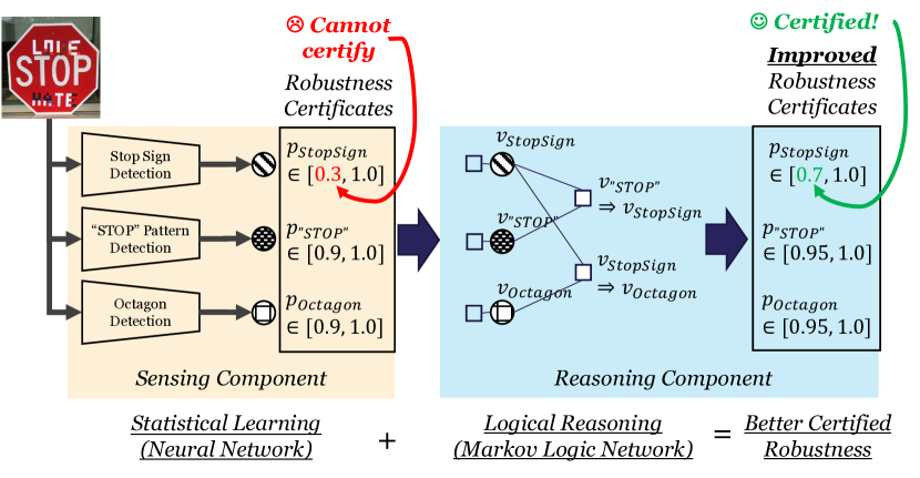
Figure 1: The sensing-reasoning pipeline, i.e., a sensing component consists of DNNs and a reasoning component is constructed as MLN. The goal of this paper is to provide certified robustness for such a pipeline, especially the reasoning component.

However, certifying the robustness of sensing-reasoning pipeline is challenging, especially given the inference complexity of the reasoning component. Our goal is to take the first step in tackling this challenge. In particular, the robustness certification of sensing-reasoning pipeline can be expressed as the confidence interval of the marginal probability for the final output of reasoning component. That is to say, we can use existing state-of-the-art methods to certify the robustness of the sensing component that contains DNNs or ensembles [8, 42, 58]. Thus, to provide the end-to-end certification for the whole pipeline, what is left is to understand how to certify the reasoning component, which is the focus of this work.

Compared with previous efforts focusing on certified robustness of neural networks, the reasoning component brings its own challenges and opportunities. Different from a neural network whose inference can be executed in polynomial time, many reasoning models such as MLN can be #P-complete for inference. However, as many reasoning models define a probability distribution in the exponential family, we have more functional structures that could potentially make the robustness optimization (which essentially solves a min-max problem) easier. In this paper, we provide the first treatment to this problem characterized by these unique challenges and opportunities.

We focus on MLN as the reasoning component, and explored three technical questions, each of which corresponds to a technical contribution of this work.

1. Is certifying robustness for the reasoning component feasible when the inference of the reasoning component is #P-hard? (Section 3) Before any concrete algorithm can be proposed, it is important to understand the computational complexity of the robustness certification. We first prove that the famous problem of counting in statistical inference [50] can be reduced to the problem of checking the certified robustness of general reasoning components and MLN. Therefore, checking certified robustness is no easier than counting on the same family of distribution. In other words, when the reasoning component is a graphical model such as MLN, checking certified robustness is no easier than calculating the partition function of the underlying graphical model, which is #P-hard.

2. Can we efficiently reason about the certified robustness for the reasoning component when given an oracle for statistical inference? (Section 4.2) Given the above hardness result, we focus on certifying the robustness given an inference oracle. However, even when statistical inference can be done by a given oracle [21, 18], it is still challenging to certify the robustness of MLN. Our second technical contribution is to develop such an algorithm for MLN as the reasoning component. We prove that providing certified robustness for MLN is possible because of the structure inherent in the probabilistic graphical models and distributions in the exponential family, which could lead to monotonicity and convexity properties under certain conditions for solving the certification optimization.

3. Can a reasoning component improve the certified robustness compared with the state-of-the-art certification methods? (Section 5) We test our algorithms on multiple sensing-reasoning pipelines, in which the sensing components contain the state-of-the-art deep neural networks. We construct these pipelines to cover a range of applications including image classification and natural language processing tasks. We show that based on our certification method on the reasoning component, the knowledge-enriched sensing-reasoning pipelines achieves significantly higher certified robustness than the state-of-the-art certification methods for DNNs.

The rest of the paper is organized as follows. We will first introduce the design of the sensing-reasoning pipeline in Section 2.1, followed by concrete illustrations taking the Markov Logic Networks as an example of the reasoning component in Section 2.2. Next, to certify the robustness of the sensing-reasoning pipeline, especially for the reasoning component, we first prove that certifying the robustness of the reasoning component itself is #P-complete (Section 3), and therefore we propose a certification algorithm to upper/lower bound the certification in Section 4, We provide the evaluation of our robustness certification considering different tasks in Section 5.

2 Robust Statistical Learning with Logical Reasoning

In this section, we first provide a sensing-reasoning pipeline and then formally defined its certified robustness, and particularly links it to certifying the robustness for the reasoning component.

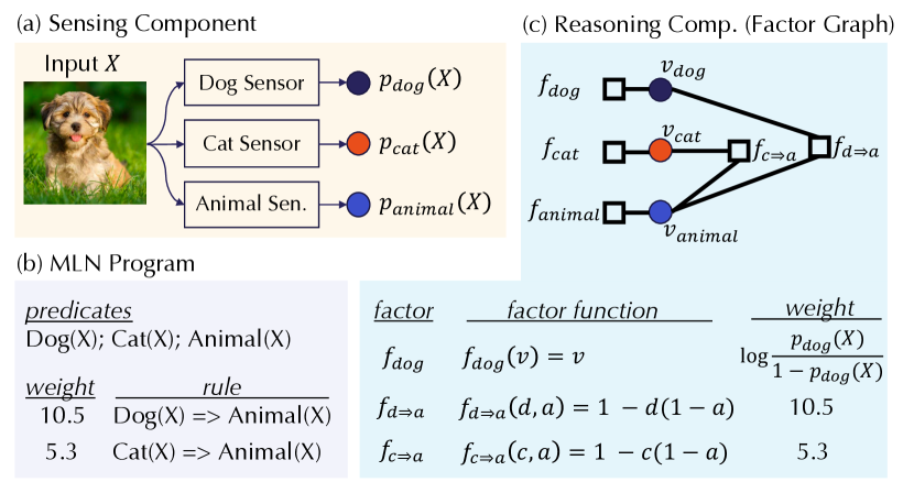
Figure 2: A sensing-reasoning pipeline with MLN as the reasoning component.

2.1 Sensing-Reasoning Pipeline

A sensing-reasoning pipeline contains a set of $n$ sensors $\{S_{i}\}_{i\in[n]}$ and a reasoning component $R$. Each sensor is a binary classifier (for multi-class classifier it corresponds to a group of sensors) — given an input data example $X$, each of the sensor $S_{i}$ outputs a probability $p_{i}(X)$ (i.e., if $S_{i}$ is a neural network, $p_{i}(X)$ represents its output after the final softmax layer). The reasoning component takes the outputs of all sensing models as its inputs, and outputs a new Boolean random variable $R(\{p_{i}(X)\}_{i\in[n]})$.

One natural choice of the reasoning component is to use a probabilistic graphical model (PGM). In the following subsection, we will make the reasoning component $R$ more concrete by instantiating it as a Markov logic network (MLN). The output of a sensing-reasoning pipeline on the input data example $X$ is the expectation of the output of reasoning component $R$: $\mathbb{E}[R(\{p_{i}(X)\}_{i\in[n]})]$.

Example. A sensing-reasoning pipeline provides a generic, principled way of integrating domain knowledge with the output of statistical predictive models such as neural networks. One such example is [10] the task of ImageNet classification. Here each sensing model corresponds to the classifier for one specific class in ImageNet, e.g., $S_{dog}(X)$ and $S_{animal}(X)$. The reasoning component then encodes domain knowledge such that “If an image is classified as a dog then it must also be classified as an animal” using a PGM. There is no prior work considering the certified robustness of such a knowledge-enabled ML pipeline. Figure 2 illustrates a concrete sensing-reasoning pipeline, in which the reasoning component is implemented as an MLN.

2.2 Reasoning Component as Markov Logic Networks

Given the generic definition of a sensing-reasoning pipeline, one can use different models to implement the reasoning components. In this paper, we focus on Markov logic networks (MLN), which is a popular way to define a probabilistic graphical model using first-order logic [41]. Concretely, we define the reasoning component implemented as an MLN, which contains a set of weighted first-order logic rules, as illustrated in Figure 2(b). After grounding, an MLN defines a joint probabilistic distribution among a collection of random variables, as illustrated in Figure 2(c). We adapt the standard MLN semantics to a sensing-reasoning pipeline and use a slightly more general variant compared with the original MLN [41]. Each MLN program corresponds to a factor graph — Due to the space limitation, we will not discuss the grounding part and point the readers to [41]. We focus on defining the result after grounding, i.e., the factor graph.

Specifically, a grounded MLN is a factor graph $\mathcal{G}=(\mathcal{V},\mathcal{F})$, where $\mathcal{V}$ is a set of Boolean random variables. Specific to a sensing-reasoning pipeline, there are two types of random variables $\mathcal{V}=\mathcal{X}\cup\mathcal{Y}$:

1. Interface Variables $\mathcal{X}=\{x_{i}\}_{i\in[n]}$: Each sensing model $S_{i}$ corresponds to one interface variable $x_{i}$ in the grounded factor graph;

2. Interior variables $\mathcal{Y}=\{y_{i}\}_{i\in[m]}$ are other variables introduced by the MLN model.

Each factor $F\in\mathcal{F}$ contains a weight $w_{F}$ and a factor function $f_{F}$ defined over a subset of variables $\bar{\bf v}_{F}\subseteq\mathcal{V}$ that returns $\{0,1\}$. There are two sets of factors $\mathcal{F}=\mathcal{G}\cup\mathcal{H}$:

1. Interface Factors $\mathcal{G}$: For each interface variable $x_{i}$, we create one interface factor $G_{i}$ with weight $w_{G_{i}}=\log[p_{i}(X)/(1-p_{i}(X))]$ and factor function $f_{G_{i}}(a)=\mathcal{I}[a=1]$ defined over $\bar{\bf v}_{f_{G_{i}}}=\{x_{i}\}$.

2. Interior Factors $\mathcal{H}$ are other factors introduced by the MLN program.

Remarks: MLN-specific Structure. Our result applies to a more general family of factor graphs and are not necessarily specific to those grounded by MLN. Moreover, MLN provides an intuitive way of grounding such a factor graph with domain knowledge, and factor graphs grounded by MLN have certain properties that we will use later, e.g., all factors only return non-negative values, and there are no unusual weight sharing structures.

The above factor graph defines a joint probability distribution among all variables $\mathcal{V}$. We define a possible world as a function $\sigma:\mathcal{V}\mapsto\{0,1\}$ that corresponds to one possible assignment of values to each random variable. Let $\Sigma$ denote the set of all (exponentially many) possible worlds.

The statistical inference process of a reasoning component implemented using MLNs [41] computes the marginal probability of a given variable $v\in\mathcal{V}$:

$$\vspace{-2mm}\mathbb{E}[R_{MLN}(\{p_{i}(X)\}_{i\in[n]})]=\mathbf{Pr}\left[v=1\right]=Z_{1}(\{p_{i}(X)\}_{i\in[n]})/Z_{2}(\{p_{i}(X)\}_{i\in[n]}$$

where the partition functions $Z_{1}$ and $Z_{2}$ are defined as

$$Z_{1}(\{p_{i}(X)\}_{i\in[n]})=\sum_{\sigma\in\Sigma\wedge\sigma(v)=1}\exp\left\{\sum_{G_{i}\in\mathcal{G}}w_{G_{i}}\sigma(x_{i})+\sum_{H\in\mathcal{H}}w_{H}f_{H}(\sigma(\bar{\bf v}_{H}))\right\}$$

$$Z_{2}(\{p_{i}(X)\}_{i\in[n]})=\sum_{\sigma\in\Sigma}\exp\left\{\sum_{G_{i}\in\mathcal{G}}w_{G_{i}}\sigma(x_{i})+\sum_{H\in\mathcal{H}}w_{H}f_{H}(\sigma(\bar{\bf v}_{H}))\right\}\vspace{-2mm}$$

Why $w_{G_{i}}=\log[p_{i}(X)/(1-p_{i}(X))]$? When the MLN does not introduce any interior variables and interior factors, it is easy to see that setting $w_{G_{i}}=\log[p_{i}(X)/(1-p_{i}(X))]$ ensures that the marginal probability of each interface variable equals to the output of the original sensing model $p_{i}(X)$. This means that if we do not have additional knowledge in the reasoning component, the pipeline outputs the same distribution as the original sensing component.

Learning Weights for Interior Factors? In this paper, we view all weights for interior factors as hyperparameters. These weights can be learned by maximizing the likelihood with weight learning algorithms for MLNs [29].

Beyond Marginal Probability for a Single Variable. We have assumed that the output of a sensing-reasoning pipeline is the marginal probability distribution of a given random variable in the grounded factor graph. However, our result can be more general — given a function over possible worlds and outputs $\{0,1\}$, the output of a pipeline can be the marginal probability of such a function. This will not change the algorithm that we propose later.

3 Hardness of Certifying Reasoning Robustness

Given a reasoning component $R$, how hard is it to reason about its robustness? In this section, we aim at understanding this fundamental question. In order to provide the certified robustness of the reasoning component, which is defined as the lower bound of model predictions for inputs considering an adversarial perturbation with bounded magnitude [8], we need to analyze the hardness of this certification problem first. Specifically, we present the hardness results of determining the robustness of the reasoning component defined above, before we can provide our certification algorithm in Section 4.2. We start by defining the counting [50] and robustness problems on general distribution. We prove that counting can be reduced to checking for reasoning robustness, and hence the latter is at least as hard; We then prove the complexities of reasoning with MLN.

3.1 Harness of Certifying General Reasoning Model

Let $\*X=\{x_{1},x_{2},\dots,x_{n}\}$ be a set of variables. Let $\pi_{\alpha}$ be a distribution over $D^{[n]}$ defined by a set of parameters $\alpha\in P^{[m]}$, where $D$ is the domain of variables, either discrete or continuous, and $P$ is the domain of parameters. We call $\pi$ accessible if for any $\sigma\in D^{[n]}$, $\pi_{\alpha}(\sigma)\propto w(\sigma;\alpha)$, where $w:D^{[n]}\times P^{[m]}\rightarrow\mathbb{R}_{\geq 0}$ is a polynomial-time computable function. We will restrict our attention to accessible distributions only. We use $Q:D^{[n]}\rightarrow\{0,1\}$ to denote a Boolean query, which is a polynomial-time computable function. We define the following two oracles:

Definition 1 (Counting).

Given input polynomial-time computable weight function $w(\cdot)$ and query function $Q(\cdot)$, parameters $\alpha$, a real number ${\epsilon}>0$, a Counting oracle outputs a real number $Z$ that

$$1-{\epsilon}\leq\frac{Z}{\mathbb{E}[\sigma\sim\pi_{\alpha}]{Q(\sigma)}}\leq 1+{\epsilon}.$$

Definition 2 (Robustness).

Given input polynomial-time computable weight function $w(\cdot)$ and query function $Q(\cdot)$, parameters $\alpha$, two real numbers $\epsilon>0$ and $\delta>0$, a Robustness oracle decides, for any $\alpha^{\prime}\in P^{[m]}$ such that $\left\|\alpha-\alpha^{\prime}\right\|_{\infty}\leq\epsilon$, whether the following is true:

$$\small\left|\mathbb{E}[\sigma\sim\pi_{\alpha}]{Q(\sigma)}-\mathbb{E}[\sigma\sim\pi_{\alpha^{\prime}}]{Q(\sigma)}\right|<\delta.$$

We can prove that Robustness is at least as hard as Counting by a reduction argument.

Theorem 1 ($\textnormal{{Counting}}\leq_{\texttt{t}}\textnormal{{Robustness}}$).

Given polynomial-time computable weight function $w(\cdot)$ and query function $Q(\cdot)$, parameters $\alpha$ and real number ${\epsilon}>0$, the instance of Counting, $(w,Q,\alpha,{\epsilon})$ can be determined by up to $O(1/\varepsilon_{c}^{2})$ queries of the Robustness oracle with input perturbation $\epsilon=O(\varepsilon_{c})$.

Proof-sketch. We define the partition function $Z_{i}:=\sum_{\sigma:Q(\sigma)=i}w(\sigma;\alpha)$ and $\mathbb{E}[\sigma\sim\pi_{\alpha}]{Q(\sigma)}=Z_{1}/(Z_{0}+Z_{1})$. We then construct a new weight function $t(\sigma;\alpha):=w(\sigma;\alpha)\exp(\beta Q(\sigma))$ by introducing an additional parameter $\beta$, such that $\tau_{\beta}(\sigma)\propto t(\sigma;\beta)$, and $\mathbb{E}[\sigma\sim\tau_{\beta}]{Q(\sigma)}=\frac{e^{\beta}Z_{1}}{Z_{0}+e^{\beta}Z_{1}}$. Then we consider the perturbation $\beta^{\prime}=\beta\pm\epsilon$, with $\epsilon=O(\varepsilon_{c})$ and query the Robustness oracle with input $(t,Q,\beta,\epsilon,\delta)$ multiple times to perform a binary search in $\delta$ to estimate $\left|\mathbb{E}[\sigma\sim\pi_{\beta}]{Q(\sigma)}-\mathbb{E}[\sigma\sim\pi_{\beta^{\prime}}]{Q(\sigma)}\right|$. Perform a further “outer" binary search to find the $\beta$ which maximizes the perturbation. This yields a good estimator for $\log{\frac{Z_{0}}{Z_{1}}}$ which in turn gives $\mathbb{E}[\sigma\sim\pi_{\alpha}]{Q(\sigma)}$ with $\varepsilon_{c}$ multiplicative error. We leave detailed proof to Appendix A.

3.2 Hardness of Certifying Markov Logic Networks

Given Theorem 1, we can now state the following result specifically for MLNs:

Theorem 2 (MLN Hardness).

Given an MLN whose grounded factor graph is $\mathcal{G}=(\mathcal{V},\mathcal{F})$ in which the weights for interface factors are $w_{G_{i}}=\log p_{i}(X)/(1-p_{i}(X))$ and constant thresholds $\delta,\{C_{i}\}_{i\in[n]}$, deciding whether

$$\forall\{\epsilon_{i}\}_{i\in[n]}~{}~{}~{}~{}(\forall i.~{}|\epsilon_{i}|<C_{i})\implies\left|\mathbb{E}R_{MLN}(\{p_{i}(X)\}_{i\in[n]})-\mathbb{E}R_{MLN}(\{p_{i}(X)+\epsilon_{i}\}_{i\in[n]})\right|<\delta$$

is as hard as estimating $\mathbb{E}R_{MLN}(\{p_{i}(X)\}_{i\in[n]})$ up to $\varepsilon_{c}$ multiplicative error, with $\epsilon_{i}=O(\varepsilon_{c})$.

Proof.

Let $\alpha=[p_{i}(X)]$, query function $Q(.)=R_{MLN}(.)$ and $\pi_{\alpha}$ defined by the marginal distribution over interior variables of MLN. Theorem 1 directly implies that $O(1/\varepsilon_{c}^{2})$ queries of a Robustness oracle can be used to efficiently estimate $\mathbb{E}R_{MLN}(\{p_{i}(X)\}_{i\in[n]})$. ∎

In general, statistical inference in MLNs is #P-complete, and checking robustness for general MLNs is also #P-hard.

4 Certifying the Robustness of Sensing-Reasoning Pipeline

Given a sensing-reasoning pipeline with $n$ sensors $\{S_{i}\}_{i\in[n]}$ and a reasoning component $R$, we will first formally define its end-to-end certified robustness and then its connection to the robustness of each component. In particular, based on the above hardness result for certifying the robustness of the reasoning component in Section 3, we will provide an effective certification method to upper/lower bound the certification, taking any oracle for the inference of the reasoning component into account. With the certification of the reasoning component, we will finally provide the robustness certification for the sensing-reasoning pipeline by combining the certification of sensing and reasoning components.

Definition 3 ($(C_{I},C_{E},p)$-robustness).

A sensing-reasoning pipeline with $n$ sensors $\{S_{i}\}_{i\in[n]}$ and a reasoning component $R$ is $(C_{I},C_{E},p)$-robust on the input $X$, if for input perturbation $\eta,||\eta||_{p}\leq C_{I}$

$$\small\left|\mathbb{E}[R(\{p_{i}(X)\}_{i\in[n]})]-\mathbb{E}[R(\{p_{i}(X+\eta)\}_{i\in[n]})]\right|\leq C_{E}.$$

I.e., a perturbation $||\eta||_{p}<C_{I}$ on the input only changes the final pipeline output by at most $C_{E}$.

Sensing Robustness and Reasoning Robustness. We decompose the end-to-end certified robustness of the pipeline into two components. The first component, which we call the sensing robustness, has been studied by the research community recently [20, 46, 8] — given a perturbation $||\eta||_{p}<C_{I}$ on the input $X$, we say each sensor $S_{i}$ is $(C_{I},C_{S}^{(i)},p)$-robust if

$$\small\forall\eta,||\eta||_{p}\leq C_{I}\implies|p_{i}(X)-p_{i}(X+\eta)|\leq C_{S}^{(i)}$$

The robustness of the reasoning component R is defined as: Given a perturbation $|\epsilon_{i}|<C_{S}^{(i)}$ on the output of each sensor $S_{i}(X)$, we say the reasoning component $R$ is $\left(\{C_{S}^{(i)}\}_{i\in[n]},C_{E}\right)$-robust if

$$\vspace{-3mm}\forall\epsilon_{1},...,\epsilon_{n},(\forall i.~{}|\epsilon_{i}|\leq C_{S}^{(i)})\implies\left|\mathbb{E}[R(\{p_{i}(X)\}_{i\in[n]})]-\mathbb{E}[R(\{p_{i}(X)+\epsilon_{i}\}_{i\in[n]})]\right|\leq C_{E}.$$

It is easy to see that when the sensing component is $\left(C_{I},\{C_{S}^{(i)}\}_{i\in[n]},p\right)$-robust and the reasoning component is $\left(\{C_{S}^{(i)}\}_{i\in[n]},C_{E}\right)$-robust on $X$, the sensing-reasoning pipeline is $(C_{I},C_{E},p)$-robust. Since the sensing robustness has been intensively studied by previous work, in this paper, we mainly focus on the reasoning robustness and therefore analyze the robustness of the pipeline.

4.1 Certifying Sensing Robustness

There are several existing ways to certify the robustness of sensing models, such as Interval Bound Propagation (IBP) [16], Randomized Smoothing [8], and others [64, 52]. Here we will leverage randomized smoothing to provide an example for certifying the robustness of sensing components.

Corollary 1.

Given a sensing model $S_{i}$, we construct a smoothed sensing model $g_{i}(X;\hat{\sigma})=\mathbb{E}_{\xi\sim\mathcal{N}(0,\hat{\sigma}^{2})}p_{i}(X+\xi)$. With input perturbation $||\eta||_{2}\leq C_{I}$, the smoothed sensing model satisfies

$$\Phi(\Phi^{-1}(g_{i}(X;\hat{\sigma}))-C_{I}/\hat{\sigma}) \leq g_{i}(X+\eta;\hat{\sigma})\leq\Phi(\Phi^{-1}(g_{i}(X;\hat{\sigma}))+C_{I}/\hat{\sigma})\vspace{-2mm}$$

where $\Phi$ is the Gaussian CDF and $\Phi^{-1}$ as its inverse.

Thus, the output probability of smoothed sensing model can be bounded given input perturbations. Note that the specific ways of certifying sensing robustness is orthogonal to certifying reasoning robustness, and one can plug in different sensing certification strategies.

4.2 Certifying Reasoning Robustness

Given the hardness results for certifying reasoning robustness in Section 3.2, in this paper, we assume that we have access to an oracle for statistical inference, and provide a novel algorithm to certify the reasoning robustness. I.e., we assume that we are able to calculate the two partition functions $Z_{1}(\{p_{i}(X)\}_{i\in[n]})$ and $Z_{2}(\{p_{i}(X)\}_{i\in[n]})$.

Lemma 4.1 (MLN Robustness).

Given access to partition functions $Z_{1}(\{p_{i}(X)\}_{i\in[n]})$ and $Z_{2}(\{p_{i}(X)\}_{i\in[n]})$, and maximum perturbations $\{C_{i}\}_{i\in[n]}$, $\forall\epsilon_{1},...,\epsilon_{n}$, if $\forall i.~{}|\epsilon_{i}|<C_{i}$, we have that $\forall\lambda_{1},...,\lambda_{n}\in\mathbb{R}$,

$$\max_{\{|\epsilon_{i}|<C_{i}\}}\ln\mathbb{E}[R_{MLN}(\{p_{i}(X)+\epsilon_{i}\}_{i\in[n]})]\leq\max_{\{|\epsilon_{i}|<C_{i}\}}\widetilde{Z_{1}}(\{\epsilon_{i}\}_{i\in[n]})-\min_{\{|\epsilon_{i}^{\prime}|<C_{i}\}}\widetilde{Z_{2}}(\{\epsilon_{i}^{\prime}\}_{i\in[n]})$$

$$\min_{\{|\epsilon_{i}|<C_{i}\}}\ln\mathbb{E}[R_{MLN}(\{p_{i}(X)+\epsilon_{i}\}_{i\in[n]})]\geq\min_{\{|\epsilon_{i}|<C_{i}\}}\widetilde{Z_{1}}(\{\epsilon_{i}\}_{i\in[n]})-\max_{\{|\epsilon_{i}^{\prime}|<C_{i}\}}\widetilde{Z_{2}}(\{\epsilon_{i}^{\prime}\}_{i\in[n]})\vspace{-2mm}$$

where

$$\widetilde{Z_{r}}(\{\epsilon_{i}\}_{i\in[n]})=\ln Z_{r}(\{p_{i}(X)+\epsilon_{i}\}_{i\in[n]})+\sum_{i}\lambda_{i}\epsilon_{i}.$$

We leave the proof to the Appendix B. The high-level proof idea is to decouple $Z_{1}/Z_{2}$ into two sub-problems via a collection of Lagrangian multipliers, i.e., $\{\lambda_{i}\}$. For any assignment of $\{\lambda_{i}\}$, we obtain a valid upper/lower bound, which reduces the certification process to the process of searching for an assignment of these multipliers that minimize the upper bound (maximize the lower bound).

To efficiently search for the optimal assignment of $\{\lambda_{i}\}$, it is crucial to consider the interactions between these $\{\lambda_{i}\}$ and the corresponding solution of $\widetilde{Z_{r}}$, which hinges on the structure of MLN. In particular, we can prove the following (Detailed proofs and discussions in Appendix C):

Proposition 1 (Monotonicity).

When $\lambda_{i}\geq 0$, $\widetilde{Z_{r}}(\{\epsilon_{i}\}_{i\in[n]})$ monotonically increases w.r.t. $\epsilon_{i}$; When $\lambda_{i}\leq-1$, $\widetilde{Z_{r}}(\{\epsilon_{i}\}_{i\in[n]})$ monotonically decreases w.r.t. $\epsilon_{i}$.

Proposition 2 (Convexity).

$\widetilde{Z_{r}}(\{\tilde{\epsilon}_{i}\}_{i\in[n]})$ is a convex function in $\tilde{\epsilon}_{i},\forall i$ with

$$\tilde{\epsilon}_{i}=\log\left[\frac{(1-p_{i}(X))(p_{i}(X)+\epsilon_{i})}{p_{i}(X)(1-p_{i}(X)-\epsilon_{i})}\right].$$

Implication. Given the monotonicity region, the maximal and minimal of $\widetilde{Z_{r}}$ are achieved at either $\epsilon_{i}=-C_{i}$ or $\epsilon_{i}=C_{i}$ respectively. Given the convexity region, the maximal is achieved at $\epsilon_{i}\in\{-C_{i},C_{i}\}$, and the minimal is achieved at $\epsilon_{i}\in\{-C_{i},C_{i}\}$ or at the zero gradient of $\widetilde{Z_{r}}(\{\tilde{\epsilon}_{i}\}_{i\in[n]})$. As a result, our analysis leads to the following certification algorithm.

Algorithm 1 Algorithms for MLN robustness upper bound (algorithm of lower bound is similar)

0: : Oracles calculating $\widetilde{Z_{1}}$ and $\widetilde{Z_{2}}$; maximal perturbations $\{C_{i}\}_{i\in[n]}$.

0: : An upper bound for input $R_{MLN}(\{p_{i}(X)+\epsilon_{i}\})$

1: $\overline{R}_{min}\leftarrow 1$

2: initialize $\lambda$

3: for $b\in\text{search budgets}$ do

4:    $\lambda\rightarrow\texttt{update}(\{\lambda\};\lambda_{i}\in(-\infty,-1]\cup[0,+\infty))$

5:    for $i=1$ to $n$ do

6:       if $\lambda_{i}\geq 0$ then

7:          $\epsilon_{i}=C_{i}$, $\epsilon^{\prime}_{i}=-C_{i}$

8:       else if $\lambda_{i}\leq-1$ then

9:          $\epsilon_{i}=-C_{i}$, $\epsilon^{\prime}_{i}=C_{i}$

10:       end if

11:       $\overline{R}\leftarrow\widetilde{Z_{1}}(\{\epsilon_{i}\}_{i\in[n]})-\widetilde{Z_{2}}(\{\epsilon_{i}^{\prime}\}_{i\in[n]})$

12:       $\overline{R}_{min}\leftarrow\min(\overline{R}_{min},\overline{R})$

13:    end for

14: end for

15: return $\overline{R}_{min}$

Algorithm of Certifying Reasoning Robustness. Algorithm 1 illustrates the detailed algorithm based on the above result to upper bound the robustness of MLN. The main step is to explore different regimes of the $\{\lambda_{i}\}$. In this paper, we only explore regimes where $\lambda\in(-\infty,-1]\cup[0,+\infty)$ as this already provides reasonable solutions in our experiments. The function $\texttt{update}(\{\lambda_{i}\})$ defines the exploration strategy — Depending on the scale of the problem, one can explore $\{\lambda_{i}\}$ using grid search, random sampling, or even gradient-based methods. For experiments in this paper, we use either grid search or random sampling. It is an exciting future direction to understand other efficient exploration and search strategies. We leave the detailed explanation of the algorithm to LABEL:{apx:sup_alg1}.

5 Experiments

We conduct intensive experiments on five datasets to evaluate the certified robustness of the sensing-reasoning pipeline. We focus on two tasks with different modalities: image classification task on Road Sign dataset created based on GTSRB dataset [45] following the standard setting as [17]; and information extraction task with stocks news on text data. We also report additional results on two other image classification tasks (Word50 [6] and PrimateNet, which is a subset of ImageNet ILSVRC2012 [9]) with natural knowledge rules in Appendix G and Appendix F. We also report results on standard image benchmarks (MNIST and CIFAR10) with manually constructed knowledge rules in Appendix H. The code is provided at https://github.com/Sensing-Reasoning/Sensing-Reasoning-Pipeline.

5.1 Experimental Setup

Datasets and Tasks. For the road sign classification task, we follow [17] and use the same dataset GTSRB [45], which contains 12 types of German road signs {"Stop”, "Priority Road”, "Yield”, "Construction Area”, "Keep Right”, "Turn Left”, "Do not Enter”, "No Vihicles”, "Speed Limit 20”, "Speed Limit 50”, "Speed Limit 120”, "End of Previous Limitation”}. It consists of 14880 training samples, 972 validation samples, and 3888 testing samples. We also include 13 additional detectors for knowledge integration, detecting attributes such as whether the border has an octagon shape (See Appendix D for a full list).

For the information extraction task, we use the HighTech dataset which consists of both daily closing asset price and financial news from 2006 to 2013 [12]. We choose 9 companies with the most news, resulting in 4810 articles related to 9 stocks filtered by company name. We split the dataset into training and testing days chronologically. We define three information extraction tasks as our sensing models: StockPrice(Day, Company, Price), StockPriceChange(Day, Company, Percent), StockPriceGain(Day, Company). The domain knowledge that we integrate depicts the relationships between these relations (See Appendix E for more details).

Knowledge Rules. We integrate different types of knowledge rules for these two applications. We provide the full list of knowledge rules in the Appendix D.

For road sign classification, we follow [17], which includes two different types of knowledge rules — Indication rules (road sign class $u$ indicates attribute $v$) and Exclusion rules (attribute classes $u$ and $v$ with the same general type such as "Shape”, "Color”, "Digit” or "Content” are naturally exclusive).

For information extraction, we integrate knowledge about the relationships between the sensing models (e.g., StockPrice, StockPriceChange, StockPriceGain). For example, the stock prices of two consecutive days, $\texttt{StockPrice}(d_{1},Company,p_{1})$ and $\texttt{StockPrice}(d_{2},Company,p_{2})$, should be consistent with $\texttt{StockPriceChange}(d_{2},Company,p)$, i.e., $p=(p_{2}-p_{1})/p_{1}$.

Implementation Details. Throughout the road sign classification experiment, we implement all sensing models using the GTSRB-CNN [13] architecture. During training, we train all sensors with Isotropic Gaussian $\epsilon\sim\mathcal{N}(0,\hat{\sigma}^{2}I_{d})$ augmented data with 50000 training iterations until converge and tune the training parameters on the validation set, following [8]. We use the SGD-momentum with the initial learning rate as $0.01$ and the weight decay parameter as $10^{-4}$ to train all the sensors for 50000 iterations with $200$ as the batch size, following [17]. During certification, we adopt the same smoothing parameter for training to construct the smoothed model based on Monte-Carlo sampling.

For information extraction, we use BERT as our model architecture. During training, we use the final hidden state of the first token [CLS] from BERT as the representation of the whole input and apply dropout with probability $p=0.5$ on this final hidden state. Additionally, there is a fully connected layer added on top of BERT for classification. To fine-tune the BERT classifiers for three information tasks, we use the Adam optimizer with the initial learning rate as $10^{-5}$ and the weight decay parameter as $10^{-4}$. We train all the sensors for 30 epochs, and the batch size $32$.

Evaluation Metrics. We adopt the standard certified accuracy as our evaluation metric, defined by the percentage of instances that can be certified under certain $\ell_{p}$-norm bounded perturbations. Specifically, given the input $x$ with ground-truth label $y$, once we can certify the bound of the model’s output confidence on predicting label $y$ under the norm-bounded perturbation as $[\mathcal{L},\mathcal{U}]$, the certified accuracy can be defined by: $\frac{1}{N}\sum_{i=1}^{N}\mathbbm{I}([\mathcal{L}_{i}>0.5])$ where $\mathbbm{I(\cdot)}$ denotes the indicator function. Since each sensing component’s certification is performed by randomized smoothing, which yields the failure probability characterized by $\zeta_{0}$, we will control the failure probability $\zeta$ for the whole sensing-reasoning pipeline pipeline with $n$ sensing models as $\zeta_{0}=1-(1-\zeta)^{1/n}$ by applying the union bound. Throughout all the experiments, $\zeta$ is kept to $0.001$ so our end-to-end certification is guaranteed to be correct with at least $99.9\%$ confidence.

Table 1: (Road sign classification) Certified accuracy under different input perturbation magnitudes ($C_{I}$). Models are smoothed with different Gaussian noises $\epsilon\sim\mathcal{N}(0,\hat{\sigma}^{2}I_{d}),\hat{\sigma}\in\{0.12,0.25,0.50\}$. Rows with $\ast$ denote the best certified accuracy among all the smoothing parameters for each method. The bold numbers show the higher certified accuracy under the same $(C_{I},\hat{\sigma})$ setting and the numbers with underline show the highest certified accuracy for each $C_{I}$ among different smoothing parameters. (All certificates hold with $p=99.9\%$)

Methods	$\hat{\sigma}$	$C_{I}=0.12$	$C_{I}=0.25$	$C_{I}=0.50$	$C_{I}=1.00$
	0.12	90.8	87.1	0.0	0.0
Vanilla Smoothing	0.25	89.6	88.4	71.6	0.0
(w/o knowledge)	0.50	84.0	80.2	73.2	61.7
	$\ast$	90.8	88.4	73.2	61.7
	0.12	96.0	89.0	73.2	24.2
Sensing-Reasoning Pipeline	0.25	93.4	91.0	74.0	49.2
(w/ knowledge)	0.50	89.3	85.4	75.5	62.5
	$\ast$	96.0	91.0	75.5	62.5

5.2 Results of Road Sign Classification

In this section, we evaluate the certified robustness of our sensing-reasoning pipeline under the $\ell_{2}$-norm bounded perturbation. We first report the $\ell_{2}$ certified accuracy of our sensing-reasoning pipeline and compare it to a strong baseline as a vanilla randomized smoothing trained model (without knowledge). Note that it is flexible to replace the sensing component with other robust training algorithms. We conduct our evaluation under different smoothing parameters $\hat{\sigma}=\{0.12,0.25,0.50\}$ and various $\ell_{2}$ perturbation magnitudes on the input image $C_{I}=\{0.12,0.25,0.50,1.00\}$ (Table 1). During certification, we evaluate our certification time per sample with 25 sensors as 5.39s, which shows that the overall certification time is generally acceptable.

As shown in Table 1, we can see that with knowledge integration, sensing-reasoning pipeline achieves consistently higher certified accuracy compared to the baseline smoothed ML model without knowledge under all the perturbation magnitudes $C_{I}$ and smoothing parameter $\hat{\sigma}$ settings. Under the small perturbation magnitude cases, our improvement is very significant (around $5\%$). More interestingly, given large $C_{I}$ but small smoothing parameter $\hat{\sigma}$, vanilla randomized smoothing-based certification directly fails ($0\%$ certified accuracy) due to the looseness of the hypothesis testing bound, while the sensing-reasoning pipeline could still achieve reasonable certified robustness (over $71\%$ on $C_{I}=0.50$, $49\%$ on $C_{I}=1.00$) under the same $(C_{I},\hat{\sigma})$ settings. This indicates a very realistic case: we always under-estimate the attacker’s ability easily under the real-world setting – in this case, the sensing-reasoning pipeline could remain robust even provide reasonable certified accuracy with a conservative smoothing parameter.

5.3 Results of Information Extraction

In this section, we conduct the certified robustness evaluation on the information extraction task on text data. Since there is no good certification method on discrete NLP data for sensing models, we directly assume the maximal perturbation on the output of sensors ($C_{S}$).

Table 2: (Information extraction) Certified accuracy under different perturbation magnitudes ($C_{S}$) based on the sensing models’ output uncertainty. (All certificates hold with 99.9% confidence)

Methods	$C_{S}=0.1$	$C_{S}=0.5$	$C_{S}=0.9$
Vanilla Smoothing (w/o knowledge)	99.7	94.7	38.4
Sensing-Reasoning Pipeline (w/ knowledge)	100.0	100.0	58.8

Table 2 shows the certified accuracy on the final outputs of the reasoning component. We see that the sensing-reasoning pipeline provides significantly higher certified robustness, and even under a high perturbation magnitude on all sensing models’ output confidence ($C_{S}=0.5$), which means the sensing-reasoning pipeline can still leverage the knowledge to help enhance the robustness given strong attacker. To further illustrate intuitively why such knowledge-based reasoning helps, Figure 3 shows the “margin” — the probability of the ground truth class minus the probability of the wrong class — with or without knowledge integration. We see that, with knowledge integration, we can significantly increase the number of examples with a large “margin” under adversarial perturbations. This explains the improvement of certified robustness, which highly relies on such prediction confident margin.

We also conduct experiments on PrimateNet, Word50, MNIST, CIFAR10 datasets for the image classification tasks in Appendix F- Appendix H. We observe similar results that knowledge integration significantly boosts the certified robustness.

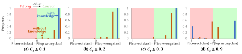
Figure 3: (Information extraction) Histogram of the robustness margin (the difference between the probability of the correct class (lower bound) and the top wrong class (upper bound)) under perturbations. If such a difference is positive, it means that the classifier makes the right prediction under perturbations.

6 Related Work

Robustness for Single ML model and ML Ensemble. Lots of efforts have been made to improve the robustness of single ML or ensemble models. Adversarial training  [15], and its variations [48, 31, 54] have generally been more successful in practice, but usually come at the cost of accuracy and increased training time [49, 54]. To further provide certifiable robustness guarantees for ML models, various certifiable defenses and robustness verification approaches have been proposed [20, 46, 8, 27, 25]. Among these strategies, randomized smoothing [8] has achieved scalable performance. With improvements in training, including pretraining and adversarial training, the certified robustness bound can be further improved [4, 42]. In addition to the single ML model, some work proposed to promote the diversity of classifiers and therefore develop a robust ML ensemble [34, 60, 58, 59]. Although promising, these defense approaches, either empirical or theoretical, can only improve the robustness of a single ML or ensemble model. Certifying or improving the robustness of such single or pure ensemble models is very challenging, given that there is no additional information that can be utilized. In addition, the ML learning process usually favors a pipeline that is able to incorporate different sensing components as well as domain knowledge in practice. Thus, certifying the robustness of such pipelines is of great importance.

Robustness of End-to-end ML Systems. There have been intensive studies on joint inference between multiple models, and the predictions based on joint inference can help to further improve the clean accuracy of ML pipelines [56, 10, 38, 33, 7, 5], which have been applied to a range of real-world applications [2, 37, 32]. Often, these approaches use different statistical inference models such as factor graphs [51], Markov logic networks [41], and Bayesian networks [35] as a way to integrate domain knowledge. In this paper, we take a different perspective on this problem — instead of treating joint inference as a way to improve the clean accuracy, we explore the possibility of using it as exogenous information to improve the end-to-end certified robustness of ML pipelines. A recent work [17] explores the empirical robustness improvement via knowledge integration, while there is no robustness guarantee provided. As we show in this paper, by integrating domain knowledge, we are able to improve the certified robustness of the ML pipelines significantly.

7 Conclusions

We provide the first certifiably robust sensing-reasoning pipeline with knowledge-based logical reasoning. We theoretically prove the certified robustness of such ML pipelines, and provide complexity analysis for certifying the reasoning component. Our extensive empirical results demonstrate the certified robustness of sensing-reasoning pipeline, and we believe our work would shed light on future research towards improving and certifying robustness for general ML frameworks as well as different ways to integrate logical reasoning with statistical learning.

Acknowledgements

This work is partially supported by the NSF grant No.1910100, NSF CNS No.2046726, C3 AI, and the Alfred P. Sloan Foundation. CZ and the DS3Lab gratefully acknowledge the support from the Swiss State Secretariat for Education, Research and Innovation (SERI) under contract number MB22.00036 (for European Research Council (ERC) Starting Grant TRIDENT 101042665), the Swiss National Science Foundation (Project Number 200021_184628, and 197485), Innosuisse/SNF BRIDGE Discovery (Project Number 40B2-0_187132), European Union Horizon 2020 Research and Innovation Programme (DAPHNE, 957407), Botnar Research Centre for Child Health, Swiss Data Science Center, Alibaba, Cisco, eBay, Google Focused Research Awards, Kuaishou Inc., Oracle Labs, Zurich Insurance, and the Department of Computer Science at ETH Zurich. HG has received funding from the European Research Council (ERC) under the European Union’s Horizon 2020 research and innovation programme (grant agreement No. 947778).

Checklist

1. For all authors…

   1. Do the main claims made in the abstract and introduction accurately reflect the paper’s contributions and scope? [Yes]

   2. Did you describe the limitations of your work? [Yes] We have mentioned the future improvement of our work in the related work part.

   3. Did you discuss any potential negative societal impacts of your work? [Yes] This work will not infer obvious negative societal impacts.

   4. Have you read the ethics review guidelines and ensured that your paper conforms to them? [Yes]

2. If you are including theoretical results…

   1. Did you state the full set of assumptions of all theoretical results? [Yes] The assumptions have been all mentioned in the main paper and appendices.

   2. Did you include complete proofs of all theoretical results? [Yes] The whole proofs are provided in Appendix A - C.

3. If you ran experiments…

   1. Did you include the code, data, and instructions needed to reproduce the main experimental results (either in the supplemental material or as a URL)? [Yes] The code is provided at https://github.com/Sensing-Reasoning/Sensing-Reasoning-Pipeline.

   2. Did you specify all the training details (e.g., data splits, hyperparameters, how they were chosen)? [Yes] All the training details have been provided in the Appendix D - I.

   3. Did you report error bars (e.g., with respect to the random seed after running experiments multiple times)? [Yes] The confidence of the reported certification results in the paper is guaranteed to be at least $99.9\%$, as mentioned in our main paper.

   4. Did you include the total amount of compute and the type of resources used (e.g., type of GPUs, internal cluster, or cloud provider)? [Yes] The detailed information is mentioned in Appendix D.

4. If you are using existing assets (e.g., code, data, models) or curating/releasing new assets…

   1. If your work uses existing assets, did you cite the creators? [Yes]

   2. Did you mention the license of the assets? [Yes]

   3. Did you include any new assets either in the supplemental material or as a URL? [Yes]

   4. Did you discuss whether and how consent was obtained from people whose data you’re using/curating? [Yes] We only use public and commonly used data.

   5. Did you discuss whether the data you are using/curating contains personally identifiable information or offensive content? [Yes] We only use public and commonly used data.

5. If you used crowdsourcing or conducted research with human subjects…

   1. Did you include the full text of instructions given to participants and screenshots, if applicable? [N/A]

   2. Did you describe any potential participant risks, with links to Institutional Review Board (IRB) approvals, if applicable? [N/A]

   3. Did you include the estimated hourly wage paid to participants and the total amount spent on participant compensation? [N/A]

Appendix A Hardness of General Distribution

We first recall the following definitions:

Counting. Given input polynomial-time computable weight function $w(\cdot)$ and query function $Q(\cdot)$, parameters $\alpha$, a real number ${\epsilon}>0$, a Counting oracle outputs a real number $Z$ such that

$$1-{\epsilon}\leq\frac{Z}{\mathbb{E}[\sigma\sim\pi_{\alpha}]{Q(\sigma)}}\leq 1+{\epsilon}.$$

Robustness. Given input polynomial-time computable weight function $w(\cdot)$ and query function $Q(\cdot)$, parameters $\alpha$, two real numbers $\epsilon>0$ and $\delta>0$, a Robustness oracle decides, for any $\alpha^{\prime}\in P^{[m]}$ such that $\left\|\alpha-\alpha^{\prime}\right\|_{\infty}\leq\epsilon$, whether the following is true:

$$\left|\mathbb{E}[\sigma\sim\pi_{\alpha}]{Q(\sigma)}-\mathbb{E}[\sigma\sim\pi_{\alpha^{\prime}}]{Q(\sigma)}\right|<\delta.$$

Proof of Theorem 1

Theorem 1 ($\textnormal{{Counting}}\leq_{\texttt{t}}\textnormal{{Robustness}}$).

Given polynomial-time computable weight function $w(\cdot)$ and query function $Q(\cdot)$, parameters $\alpha$ and real number ${\epsilon}>0$, the instance of Counting, $(w,Q,\alpha,{\epsilon})$ can be determined by up to $O(1/\varepsilon_{c}^{2})$ queries of the Robustness oracle with input perturbation $\epsilon=O(\varepsilon_{c})$.

Proof.

Let $(w,Q,\alpha,{\epsilon})$ be an instance of Counting. Define a new distribution $\tau_{\beta}$ over $\*X$ with a single parameter $\beta\in\mathbb{R}$ such that $\tau_{\beta}(\sigma)\propto t(\sigma;\beta),$ where $t(\sigma;\beta)=w(\sigma;\alpha)\exp(\beta Q(\sigma)).$ Since $Q$ is polynomial-time computable, $\tau_{\beta}$ is accessible for any $\beta$. We will choose $\beta$ later. For $i\in\{0,1\}$, define $Z_{i}:=\sum_{\sigma:Q(\sigma)=i}w(\sigma;\alpha).$ Then we have

$$\mathbb{E}[\sigma\sim\pi_{\alpha}]{Q(\sigma)}=\frac{Z_{1}}{Z_{0}+Z_{1}},\quad\mathbb{E}[\sigma\sim\tau_{\beta}]{Q(\sigma)}=\frac{e^{\beta}Z_{1}}{Z_{0}+e^{\beta}Z_{1}}.$$

We further define

$$Y^{+}(\beta,x) :=\mathbb{E}[\sigma\sim\tau_{\beta+x}]{Q(\sigma)}-\mathbb{E}[\sigma\sim\tau_{\beta}]{Q(\sigma)}$$

$$=\frac{e^{x}e^{\beta}Z_{1}}{Z_{0}+e^{x}e^{\beta}Z_{1}}-\frac{e^{\beta}Z_{1}}{Z_{0}+e^{\beta}Z_{1}}$$

$$=\frac{(e^{x}-1)e^{\beta}Z_{0}Z_{1}}{(Z_{0}+e^{x}e^{\beta}Z_{1})(Z_{0}+e^{\beta}Z_{1})}=\frac{(e^{x}-1)e^{\beta}}{R+(e^{x}+1)e^{\beta}+\frac{e^{x}e^{2\beta}}{R}},$$

where $R:=\frac{Z_{0}}{Z_{1}}$, and similarly

$$Y^{-}(\beta,x) :=\mathbb{E}[\sigma\sim\tau_{\beta}]{Q(\sigma)}-\mathbb{E}[\sigma\sim\tau_{\beta-x}]{Q(\sigma)}$$

$$=\frac{e^{\beta}Z_{1}}{Z_{0}+e^{\beta}Z_{1}}-\frac{e^{-x}e^{\beta}Z_{1}}{Z_{0}+e^{-x}e^{\beta}Z_{1}}$$

$$=\frac{(1-e^{-x})e^{\beta}Z_{0}Z_{1}}{(Z_{0}+e^{-x}e^{\beta}Z_{1})(Z_{0}+e^{\beta}Z_{1})}=\frac{(e^{x}-1)e^{\beta}}{e^{x}R+(e^{x}+1)e^{\beta}+\frac{e^{2\beta}}{R}}.$$

Easy calculation implies that for $x>0$, $Y^{+}(\beta,x)>Y^{-}(\beta,x)$ if and only if $R>e^{\beta}$. Note that

$$Y^{+}(\beta,x) =\frac{e^{x}-1}{Re^{-\beta}+e^{x}+1+\frac{e^{x+\beta}}{R}}\leq\frac{e^{x/2}-1}{e^{x/2}+1};$$

$$Y^{-}(\beta,x) =\frac{e^{x}-1}{Re^{x-\beta}+e^{x}+1+\frac{e^{\beta}}{R}}\leq\frac{e^{x/2}-1}{e^{x/2}+1}.$$

The two maximum are achieved when $R=e^{\beta\pm x/2}$. We will choose $x=O({\epsilon})$. Define

$$Y(\beta):= \max\{Y^{+}(\beta,x),Y^{-}(\beta,x)\}$$

$$= \begin{cases}\frac{e^{x}-1}{Re^{-\beta}+e^{x}+1+\frac{e^{x+\beta}}{R}}&\text{if $e^{\beta}<R$;}\\ \frac{e^{x}-1}{Re^{x-\beta}+e^{x}+1+\frac{e^{\beta}}{R}}&\text{if $e^{\beta}\geq R$.}\\ \end{cases}$$

This function $Y$ is increasing in $[0,\log R-x/2]$, decreasing in $[\log R-x/2,\log R]$, increasing in $[\log R,\log R+x/2]$ again, and decreasing in $[\log R+x/2,\infty)$ once again.

Our goal is to estimate $R$. For any fixed $\beta$, we will query the Robustness oracle with parameters $(t,Q,\beta,x,\delta)$. Using binary search in $\delta$, we can estimate the function $Y(\beta)$ above efficiently with additive error ${\epsilon}^{\prime}$ with at most $O(\log\frac{1}{{\epsilon}^{\prime}})$ oracle calls. We use binary search once again in $\beta$ so that it stops only if $Y(\beta_{0})\geq\frac{e^{x/2}-1}{e^{x/2}+1}-\varepsilon_{0}$ for some $\beta_{0}$ and the accuracy $\varepsilon_{0}\leq\frac{e^{x/2}-1}{2(e^{x/2}+1)}$ is to be fixed later. In particular, $Y(\beta_{0})\geq\frac{e^{x/2}-1}{2(e^{x/2}+1)}$. Note that here $\varepsilon_{0}$ is the accumulated error from binary searching twice.

We claim that $\beta_{0}$ is a good estimator for $\log R$. First assume that $e^{\beta_{0}}<R$, which implies that

$$\frac{e^{x/2}-1}{e^{x/2}+1}-Y(\beta_{0}) =\frac{e^{x/2}-1}{e^{x/2}+1}-\frac{e^{x}-1}{Re^{-\beta_{0}}+e^{x}+1+\frac{e^{x+\beta_{0}}}{R}}$$

$$=\frac{(e^{x}-1)}{(e^{x/2}+1)^{2}(Re^{-\beta_{0}}+e^{x}+1+\frac{e^{x+\beta_{0}}}{R})}\times$$

$$~{}~{}~{}~{}\left(\sqrt{Re^{-\beta_{0}}}-\sqrt{\frac{e^{x+\beta_{0}}}{R}}\right)^{2}$$

$$=\frac{Y(\beta_{0})}{(e^{x/2}+1)^{2}}\left(\sqrt{Re^{-\beta_{0}}}-\sqrt{\frac{e^{x+\beta_{0}}}{R}}\right)^{2}\leq\varepsilon_{0}.$$

Thus,

$$\left|\sqrt{Re^{-\beta_{0}}}-\sqrt{\frac{e^{x+\beta_{0}}}{R}}\right|\leq\sqrt{\frac{2\varepsilon_{0}(e^{x/2}+1)^{3}}{e^{x/2}-1}}.$$

Let $\rho:=Re^{-\beta_{0}}$. Note that $\rho>1$. We choose $\varepsilon_{0}:=\frac{1}{2}\left(\frac{e^{x/2}-1}{e^{x/2}+1}\right)^{3}$. Then $\left|\sqrt{\rho}-\sqrt{e^{x}/\rho}\right|<e^{x/2}-1$. If $\rho\geq e^{x}$, then $\left|\sqrt{\rho}-\sqrt{e^{x}/\rho}\right|\geq e^{x/2}-1$, a contradiction. Thus, $\rho<e^{x}$. It implies that $1<\frac{R}{e^{\beta_{0}}}<e^{x}$. Similarly for the case of $e^{\beta_{0}}>R$, we have that $e^{-x}<\frac{R}{e^{\beta_{0}}}<1$. Thus in both cases, we have our estimator $e^{-x}<\frac{R}{e^{\beta_{0}}}<e^{x}$.

Finally, to estimate $\mathbb{E}[\sigma\sim\pi_{\alpha}]{Q(\sigma)}=\frac{1}{1+R}$ with multiplicative error ${\epsilon}$, we only need to pick $x:=\log(1+{\epsilon})=O({\epsilon})$. ∎

Appendix B Robustness of MLN

Lagrange multipliers

Before proving the robustness result of MLN, we first briefly review the technique of Lagrange multipliers for constrained optimization: Consider following problem P,

$$\texttt{P:}~{}~{}~{}~{}\max_{x_{1},x_{2}}f(x_{1})+g(x_{2}),~{}~{}~{}~{}s.t.,x_{1}=x_{2},~{}~{}~{}h(x_{1}),k(x_{2})\geq 0.$$

Introducing another real variable $\lambda$, we define following problem P’,

$$\texttt{P':}~{}~{}~{}~{}\max_{x_{1},x_{2}}f(x_{1})+g(x_{2})+\lambda(x_{1}-x_{2}),~{}~{}~{}~{}s.t.,h(x_{1}),k(x_{2})\geq 0.$$

For all $\lambda$, let $(x_{1}^{*},x_{2}^{*})$ be the solution of P and let $(\bar{x_{1}},\bar{x_{2}})$ be the solution of P’, we have

$$f(x_{1}^{*})+g(x_{2}^{*})\leq f(x_{1}^{*})+g(x_{2}^{*})+\lambda(x_{1}^{*}-x_{2}^{*})\leq f(\bar{x_{1}})+g(\bar{x_{2}})+\lambda(\bar{x_{1}}-\bar{x_{2}})$$

Proof of Lemma 4.1

Lemma 4.1 (MLN Robustness).

Given access to partition functions $Z_{1}(\{p_{i}(X)\}_{i\in[n]})$ and $Z_{2}(\{p_{i}(X)\}_{i\in[n]})$, and a maximum perturbations $\{C_{i}\}_{i\in[n]}$, $\forall\epsilon_{1},...,\epsilon_{n}$, if $\forall i.~{}|\epsilon_{i}|<C_{i}$, we have that $\forall\lambda_{1},...,\lambda_{n}\in\mathbb{R}$,

$$\max_{\{|\epsilon_{i}<C_{i}|\}}\ln\mathbb{E}[R_{MLN}(\{p_{i}(X)+\epsilon_{i}\}_{i\in[n]})]\leq \max_{\{|\epsilon_{i}|<C_{i}\}}\widetilde{Z_{1}}(\{\epsilon_{i}\}_{i\in[n]})$$

$$- \min_{\{|\epsilon_{i}^{\prime}|<C_{i}\}}\widetilde{Z_{2}}(\{\epsilon_{i}^{\prime}\}_{i\in[n]})$$

$$\min_{\{|\epsilon_{i}<C_{i}|\}}\ln\mathbb{E}[R_{MLN}(\{p_{i}(X)+\epsilon_{i}\}_{i\in[n]})]\geq \min_{\{|\epsilon_{i}|<C_{i}\}}\widetilde{Z_{1}}(\{\epsilon_{i}\}_{i\in[n]})$$

$$- \max_{\{|\epsilon_{i}^{\prime}|<C_{i}\}}\widetilde{Z_{2}}(\{\epsilon_{i}^{\prime}\}_{i\in[n]})$$

where

$$\widetilde{Z_{r}}(\{\epsilon_{i}\}_{i\in[n]})=\ln Z_{r}(\{p_{i}(X)+\epsilon_{i}\}_{i\in[n]})+\sum_{i}\lambda_{i}\epsilon_{i}.$$

Proof.

Consider the upper bound, we have

$$\max_{\{|\epsilon_{i}<C_{i}|\}}\ln\mathbb{E}[R_{MLN}(\{p_{i}(X)+\epsilon_{i}\}_{i\in[n]})]= \max_{\{|\epsilon_{i}<C_{i}|\}}\ln\left(\frac{Z_{1}(\{p_{i}(X)+\epsilon_{i}\}_{i\in[n]})}{Z_{2}(\{p_{i}(X)+\epsilon_{i}\}_{i\in[n]})}\right)$$

$$= \max_{\{\epsilon_{i}\},\{\epsilon_{i}^{\prime}\}}\ln Z_{1}(\{p_{i}(X)+\epsilon_{i}\}_{i\in[n]})$$

$$-\ln Z_{2}(\{p_{i}(X)+\epsilon_{i}^{\prime}\}_{i\in[n]})$$

$$s.t.,\epsilon_{i}=\epsilon_{i}^{\prime},~{}~{}~{}~{}|\epsilon_{i}|,|\epsilon_{i}^{\prime}|\leq C_{i}.$$

Introducing Lagrange multipliers $\{\lambda_{i}\}$. Note that any choice of $\{\lambda_{i}\}$ corresponds to a valid upper bound. Thus $\forall\lambda_{1},...,\lambda_{n}\in\mathbb{R}$, we can reformulate the above into

$$\max_{\{|\epsilon_{i}<C_{i}|\}}\ln\mathbb{E}[R_{MLN}(\{p_{i}(X)+\epsilon_{i}\}_{i\in[n]})] \leq\max_{\{\epsilon_{i}\},\{\epsilon_{i}^{\prime}\}}\ln Z_{1}(\{p_{i}(X)+\epsilon_{i}\}_{i\in[n]})$$

$$-\ln Z_{2}(\{p_{i}(X)+\epsilon_{i}^{\prime}\}_{i\in[n]})$$

$$+\sum_{i}\lambda_{i}(\epsilon_{i}-\epsilon_{i}^{\prime}),$$

$$s.t.,|\epsilon_{i}|,|\epsilon_{i}^{\prime}|\leq C_{i}.$$

Define

$$\widetilde{Z_{1}}(\{\epsilon_{i}\}_{i\in[n]})=\ln Z_{1}(\{p_{i}(X)+\epsilon_{i}\}_{i\in[n]})+\sum_{i}\lambda_{i}\epsilon_{i};$$

$$\widetilde{Z_{2}}(\{\epsilon_{i}^{\prime}\}_{i\in[n]})=\ln Z_{1}(\{p_{i}(X)+\epsilon^{\prime}_{i}\}_{i\in[n]})+\sum_{i}\lambda_{i}\epsilon^{\prime}_{i},$$

We have the claimed upper-bound,

$$\max_{\{|\epsilon_{i}<C_{i}|\}}\ln\mathbb{E}[R_{MLN}(\{p_{i}(X)+\epsilon_{i}\}_{i\in[n]})]\leq \max_{\{|\epsilon_{i}|<C_{i}\}}\widetilde{Z_{1}}(\{\epsilon_{i}\}_{i\in[n]})$$

$$-\min_{\{|\epsilon_{i}^{\prime}|<C_{i}\}}\widetilde{Z_{2}}(\{\epsilon_{i}^{\prime}\}_{i\in[n]}).$$

Similarly, the lower-bound can be written in terms of Lagrange multipliers, and $\forall\lambda_{1},...,\lambda_{n}\in\mathbb{R}$, we have

$$\min_{\{|\epsilon_{i}<C_{i}|\}}\ln\mathbb{E}[R_{MLN}(\{p_{i}(X)+\epsilon_{i}\}_{i\in[n]})]\geq \min_{\{\epsilon_{i}\},\{\epsilon_{i}^{\prime}\}}\ln Z_{1}(\{p_{i}(X)+\epsilon_{i}\}_{i\in[n]})$$

$$-\ln Z_{2}(\{p_{i}(X)+\epsilon_{i}^{\prime}\}_{i\in[n]})$$

$$+\sum_{i}\lambda_{i}(\epsilon_{i}-\epsilon_{i}^{\prime}),$$

$$~{}~{}~{}~{}s.t.,|\epsilon_{i}|,|\epsilon_{i}^{\prime}|\leq C_{i}.$$

Hence we have the claimed lower-bound,

$$\min_{\{|\epsilon_{i}|<C_{i}\}}\ln\mathbb{E}[R_{MLN}(\{p_{i}(X)+\epsilon_{i}\}_{i\in[n]})]\geq \min_{\{|\epsilon_{i}|<C_{i}\}}\widetilde{Z_{1}}(\{\epsilon_{i}\}_{i\in[n]})$$

$$-\max_{\{|\epsilon_{i}^{\prime}|<C_{i}\}}\widetilde{Z_{2}}(\{\epsilon_{i}^{\prime}\}_{i\in[n]}).$$

∎

Appendix C Supplementary Results for Algorithm 1

Proposition (Monotonicity).

When $\lambda_{i}\geq 0$, $\widetilde{Z_{r}}(\{\epsilon_{i}\}_{i\in[n]})$ monotonically increases w.r.t. $\epsilon_{i}$; When $\lambda_{i}\leq-1$, $\widetilde{Z_{r}}(\{\epsilon_{i}\}_{i\in[n]})$ monotonically decreases w.r.t. $\epsilon_{i}$.

Proof.

Recall that by definition we have

$$Z_{r}(\{p_{i}(X)+\epsilon_{i}\}_{i\in[n]})=$$

$$\sum_{\sigma\in\mathcal{I}_{r}}\exp\left\{\sum_{G_{i}\in\mathcal{G}}w_{G_{i}}(p_{i}(X)+\epsilon_{i})\sigma(x_{i})+\sum_{H\in\mathcal{H}}w_{H}f_{H}(\sigma(\bar{\bf v}_{H}))\right\}$$

where $w_{G_{i}}(p_{i}(x))=\log[p_{i}(X)/(1-p_{i}(X))]$ and $\mathcal{I}_{1}=\Sigma\wedge\{\sigma(v)=1\}$ and $\mathcal{I}_{2}=\Sigma$. We can rewrite the perturbation on $p_{i}(X)$ as a perturbation on $w_{G_{i}}$: $w_{G_{i}}(p_{i}(X)+\epsilon_{i})=w_{G_{i}}+\tilde{\epsilon}_{i},$

where

$$\tilde{\epsilon}_{i}=\log\left[\frac{(1-p_{i}(X))(p_{i}(X)+\epsilon_{i})}{p_{i}(X)(1-p_{i}(X)-\epsilon_{i})}\right].$$

Note that $\tilde{\epsilon}_{i}$ is monatomic in $\epsilon_{i}$. We also have

$$\ln\mathbb{E}[R_{MLN}(\{p_{i}(X)+\epsilon_{i}\}_{i\in[n]})]=\ln\mathbb{E}[R_{MLN}(\{w_{G_{i}}(X)+\tilde{\epsilon}_{i}\}_{i\in[n]})]$$

We can hence apply the same Lagrange multiplier procedure as in the above proof of Lemma 6 and conclude that

$$\widetilde{Z_{r}}(\{\epsilon_{i}\}_{i\in[n]}):= \ln Z_{r}(\{p_{i}(X)+\epsilon_{i}\}_{i\in[n]})+\sum_{i}\lambda_{i}\epsilon_{i}$$

$$= \ln Z_{r}(\{w_{G_{i}}(X)+\tilde{\epsilon}_{i}\}_{i\in[n]})+\sum_{i}\lambda_{i}\tilde{\epsilon}_{i},$$

where $\epsilon_{i}\in[-C_{i},C_{i}]$ $\tilde{\epsilon}_{i}\in[-C_{i}^{\prime},C_{i}^{\prime}]$ with $C_{i}^{\prime}=\log\left[\frac{(1-p_{i}(X))(p_{i}(X)+C_{i})}{p_{i}(X)(1-p_{i}(X)-C_{i})}\right]$. We are now in the position to rewrite $\widetilde{Z_{r}}$ as a function of $\tilde{\epsilon}_{i}$ and obtain

$$\widetilde{Z_{r}}(\{\epsilon_{i}^{\prime}\}_{i\in[n]})$$

$$= \ln\sum_{\sigma\in\mathcal{I}_{r}}\exp\left\{\sum_{G_{i}\in\mathcal{G}}(w_{G_{i}}+\tilde{\epsilon}_{i})\sigma(x_{i})+\sum_{H\in\mathcal{H}}w_{H}f_{H}(\sigma(\bar{\bf v}_{H}))\right\}+\sum_{i}\lambda_{i}\tilde{\epsilon}_{i}$$

$$= \ln\sum_{\sigma\in\mathcal{I}_{r}}\exp\left\{\sum_{G_{i}\in\mathcal{G}}w_{G_{i}}\sigma(x_{i})+\sum_{i}(\sigma(x_{i})+\lambda_{i})\tilde{\epsilon}_{i}+\sum_{H\in\mathcal{H}}w_{H}f_{H}(\sigma(\bar{\bf v}_{H}))\right\}$$

Since $\sigma(x_{i})\in\{0,1\}$, when $\lambda_{i}\geq 0$, $\sigma(x_{i})+\lambda_{i}\geq 0$ and $\widetilde{Z_{r}}$ monotonically increases in $\tilde{\epsilon}_{i}$ and hence in $\epsilon_{i}$. When $\lambda_{i}\leq-1$, $\sigma(x_{i})+\lambda_{i}\leq 0$ and $\widetilde{Z_{r}}$ monotonically decreases in $\tilde{\epsilon}_{i}$ and hence in $\epsilon_{i}$. ∎

Proposition (Convexity).

$\widetilde{Z_{r}}(\{\tilde{\epsilon}_{i}\}_{i\in[n]})$ is a convex function in $\tilde{\epsilon}_{i},\forall i$ with

$$\tilde{\epsilon}_{i}=\log\left[\frac{(1-p_{i}(X))(p_{i}(X)+\epsilon_{i})}{p_{i}(X)(1-p_{i}(X)-\epsilon_{i})}\right].$$

Proof.

We take the second derivative of $\widetilde{Z_{r}}$ with respect to $\tilde{\epsilon}_{i}$,

$$\frac{\partial^{2}\widetilde{Z_{r}}}{\partial\epsilon_{1}^{2}}=$$

$$\frac{\sum_{\sigma\in\mathcal{I}_{r}}(\sigma(x_{i})+\lambda_{i})^{2}\exp\left\{\sum_{G_{j}\in\mathcal{G}}w_{G_{j}}\sigma(x_{j})+\sum_{j}(\sigma(x_{j})+\lambda_{j})\tilde{\epsilon}_{j}+\sum_{H\in\mathcal{H}}w_{H}f_{H}(\sigma(\bar{\bf v}_{H}))\right\}}{\sum_{\sigma\in\mathcal{I}_{r}}\exp\left\{\sum_{G_{j}\in\mathcal{G}}w_{G_{j}}\sigma(x_{j})+\sum_{j}(\sigma(x_{j})+\lambda_{j})\tilde{\epsilon}_{j}+\sum_{H\in\mathcal{H}}w_{H}f_{H}(\sigma(\bar{\bf v}_{H}))\right\}}$$

$$-$$

$$\left[\frac{\sum_{\sigma\in\mathcal{I}_{r}}(\sigma(x_{i})+\lambda_{i})\exp\left\{\sum_{G_{j}\in\mathcal{G}}w_{G_{j}}\sigma(x_{j})+\sum_{j}(\sigma(x_{j})+\lambda_{j})\tilde{\epsilon}_{j}+\sum_{H\in\mathcal{H}}w_{H}f_{H}(\sigma(\bar{\bf v}_{H}))\right\}}{\sum_{\sigma\in\mathcal{I}_{r}}\exp\left\{\sum_{G_{j}\in\mathcal{G}}w_{G_{j}}\sigma(x_{j})+\sum_{j}(\sigma(x_{j})+\lambda_{j})\tilde{\epsilon}_{j}+\sum_{H\in\mathcal{H}}w_{H}f_{H}(\sigma(\bar{\bf v}_{H}))\right\}}\right]^{2}.$$

The above is simply the variance of $\sigma(x_{i})+\lambda_{i}$, namely $\mathbb{E}\left[(\sigma(x_{i})+\lambda_{i})^{2}\right]-\mathbb{E}\left[\sigma(x_{i})+\lambda_{i}\right]^{2}\geq 0$. The convexity of $\widetilde{Z_{r}}$ in $\tilde{\epsilon}_{i}$ follows. ∎

Appendix D Image Classification on Road Sign Dataset

All the experiments shown in Appendix D - I are run on 4 RTX 2080 Ti GPUs.

Task and Dataset. For road sign classification task, the whole dataset can be viewed as a subset of GTSRB dataset [45], which contains 12 types of German road signs {"Stop”, "Priority Road”, "Yield”, "Construction Area”, "Keep Right”, "Turn Left”, "Do not Enter”, "No Vihicles”, "Speed Limit 20”, "Speed Limit 50”, "Speed Limit 120”, "End of Previous Limitation”}, with 14880 training samples, 972 validation samples and 3888 testing samples in total. Besides the road sign classes, we construct $13$ attribute classes as follows:

• Border shape classes: "Octagon”, "Square”, "Triangle”, "Circle”.

• Border color classes: "Red”, "Blue”, "Black”.

• Digit classes: "Digit 20”, "Digit 50”, "Digit 120”.

• Content classes: "Left”, "Right”, "Blank”.

Based on the indication direction from road sign classes to attribute classes, and the exclusive relationship between attribute classes with the same type, we develop the following two types of knowledge rules as follows:

• Indication rules $(u,v)$: Road sign class $u$ indicates attribute $v$.

• Exclusion rules $(u,v)$: Attribute classes $u$ and $v$ with the same type ("Shape”, "Color”, "Digit” or "Content”) are naturally exclusive. (e.g., One road sign can not have "Octagon” shape and "Triangle” shape at the same time.)

Knowledge. We construct our first-order logical rules based on our predefined indication and exclusion knowledge as follows:

• Indication edge $u\implies v$: if one object belongs to road sign class $u$, it should have attribute $u$:

  $$x_{u}\wedge\neg x_{v}=\texttt{False}$$ (1)

• Exclusion edge $u\oplus v$: On object can not have attribute $u$ and $v$ at the same time:

  $$x_{u}\land x_{v}=\texttt{False}$$ (2)

Intuitive Example. Following the HEX graph-based knowledge structure and rules, we will show several adversary scenarios which could be mitigated through the inference reasoning phase. For instance, if the “Construction Area" object is attacked to be “Stop Sign" while other sensing nodes remain unaffected, like the border shape is still detected as the “Triangle” shape. Then the indication knowledge rule (The “Stop Sign" object should have the “Octagon” border shape) and the exclusive knowledge rule (No class can have the “Triangle” border shape and “Octagon” shape at the same time) would be violated. Such violation of the knowledge rules would discourage our pipeline to predict “Stop Sign" as what the attacker wants. However, the sensing-reasoning pipeline may not distinguish the “Yield", and “Construction Area" classes if the attacker fooled the “Construction Area" sensing completely, which shows the limitation of such structural knowledge, and more knowledge would be required in this case to help improve the robustness.

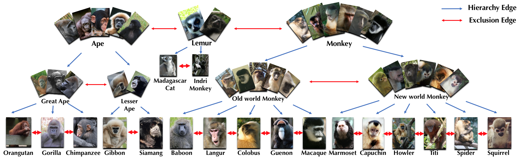
Figure 4: PrimateNet. The knowledge structure of PrimateNet dataset. The Blue arrows represent the Hierarchical rules between different classes, and the Red arrows represent the Exclusive rules. Some exclusive rules are omitted due to the space limit.

Appendix E Information Extraction on Stock News

To further evaluate the certified robustness of the reasoning component, in this section we focus on the setting where perturbations can be directly added to the output of sensors (i.e., input of the reasoning component), using information extraction task as an example.

Tasks and Dataset. We consider information extraction (or relation extraction) tasks in NLP based on the stock news dataset — HighTech dataset, which consists of both daily closing asset price and financial news from 2006 to 2013 [12]. We choose 9 companies with the highest volume of news coverage, resulting in 4810 articles related to 9 specific stocks that are filtered by company name. We split the stock news dataset into training and testing days chronologically. Here we define three information extraction tasks as sensing models: StockPrice(Day, Company, Price), StockPriceChange(Day, Company, Percent), StockPriceGain(Day, Company). The domain knowledge that we incorporate illustrates the connections between these sensing models. We provide detailed descriptions of these tasks as below.

• StockPrice(day, company, price) In this task, we extract the daily closing price of a company’s stock from the news articles. To achieve this, we first extract numbers in each sentence of the article as candidate relations. We then label each relation based on the given daily closing asset price as follows: we label the relation whose number starts with "$" and has the smallest difference with the given closing price as positive, and label all others as negative. With these labeled samples, We train a BERT-based binary classifier [11] as our sensing model to identify whether the given number is the closing price of the stock and output the prediction confidence. The input form of our BERT sensor is “[CLS] sentence [SEP] company [SEP] price”.

• StockPriceChange(day, company, percentage) In this task, we extract the percentage change in a company’s stock closing price from a collection of news articles. To achieve this, we first extract numbers in each sentence of the article as candidate relations, and label each relation using the percentage change of the closing asset price from the previous day and the current day. With these labeled samples, we train a BERT-based binary classifier as our sensing model to identify whether the given percent number represents the change rate of the stock on a given day, and output the prediction confidence. The input form of our BERT sensor is “[CLS] sentence [SEP] company [SEP] percentage”.

• StockPriceGain(day, company, gain) In this task, we extract the information about whether the closing price of a company’s stock rose or fell on a particular day given the news articles. We identify each sentence containing a stock name and numbers starting with "$" as a candidate relation, and assess each relation by counting the number of positive and negative words in the sentence to determine whether it indicates a rise or fall in the stock price. Specifically, we label one relation as positive when Count(positive word) >  Count(negative words); and negative when Count(positive word) <  Count(negative words). With these labeled samples, we train a BERT-based binary classifier as our sensing model to output the confidence. The input form of our BERT sensor is “[CLS] sentence [SEP] company”.

Implementation Details. We employ one BERT-based binary classifier for each information extraction task. To train the BERT classifiers, we adopt the final hidden state of the first token [CLS] from BERT as the representation of the whole input, and apply dropout with probability $p=0.5$ on this final hidden state. We add a fully connected layer on top of BERT for classification. To fine-tune the BERT classifiers for the three information extraction tasks, we adopt the Adam optimizer with a learning rate of $10^{-5}$, weight decay of $10^{-4}$, and train our classifiers for $30$ epochs with the batch size as $32$.

Knowledge. For each news article that pertains to a specific company, we define $d$ as the current date, $p_{1}$ as the stock price on the current date, and $p_{0}$ as the stock price on the previous day. We also use $y$ to present the binary variable that indicates whether the company’s stock price rose or fell ($y=0$ for “fell” and $y=1$ for “rose”), and $\beta$ the percentage change of stock price change. We define the following knowledge rules that the extracted tuple $(p_{0},p_{1},y,\beta)$ should satisfy:

• Rule 1: The extracted stock price $p_{0}$ and $p_{1}$ (from the StockPrice sensor) should be consistent with the stock price change indicator $y$ (from the StockPriceGain sensor):

  $$y=\mathbbm{I}[p_{1}-p_{0}>0]$$ (3)

• Rule 2: The extracted stock price $p_{0}$ and $p_{1}$ (from the StockPrice sensor) should approximately follow the percentage change of stock price $\beta$ (from the StockPriceChange sensor):

  $$p_{1}\approx p_{0}\times[1+(-1)^{\mathbbm{I}[p_{1}-p_{0}>0]}\times\beta]$$ (4)

Threat Model. Given the perturbation bound $C_{S}$, we attack our sensing-reasoning pipeline by adding perturbation $\delta$ ($\delta\leq C_{S}$) on perturbed sensing model’s confidence value $p$ directly. The perturbed confidence value, named as $p^{\prime}$, should satisfy $p^{\prime}\in[p-C_{S},p+C_{S}]$. In the threat model we consider, attackers can add perturbations to all sensing models’ output prediction confidence.

Intuitive Example. Here we show an intuitive example of how our knowledge can help improve the prediction robustness of these information extraction models under adversarial attacks. Assume our sensing models extract the correct stock price information $(p^{*}_{0},p^{*}_{1},y^{*},\beta^{*})$, where price $p^{*}_{0}>p^{*}_{1}$ and the stock price change is “fell" ($y=0$) by $\beta\%$. Now if the first stock price extraction sensor is attacked to output an incorrect prediction $p^{\prime}_{0}$ such that $p^{\prime}_{0}<p^{*}_{1}$ while other sensors remain intact; $p^{\prime}_{0}$ will violate our knowledge rules 1 and 2. Specifically, the stock price change $p^{\prime}_{0}-p^{*}_{1}<0$ is inconsistent with stock price change prediction $y=0$, i.e., $p^{\prime}_{0}-p^{*}_{1}>0$. As a result, our reasoning component will reduce the confidence of the wrong prediction $p^{\prime}_{0}$ and increase the confidence of the ground truth $p^{*}_{0}$ to be consistent with the knowledge rules; and therefore potentially recover the correct prediction of $p^{*}_{0}$.

Appendix F Image Classification on PrimateNet Dataset

Task and Dataset. We aim to evaluate the certified robustness of our sensing-reasoning pipeline on large-scale dataset such as ImageNet ILSVRC2012 [9]. In particular, to obtain domain knowledge for the images, we select 18 Primate animal categories to form a PrimateNet dataset, containing {Orangutan, Gorilla, Chimpanzee, Gibbon, Siamang, Madagascar cat, Woolly indris, Guenon, Baboon, Macaque, Langur, Colobus, Marmosets, Capuchin monkey, Howler monkey, Titi monkey, Spider monkey, Squirrel monkey}. Moreover, we create 7 internal classes {Greater ape, Lesser ape, Ape, Lemur, Old-world monkey, New-world monkey, Monkey} to construct the hierarchical structure according to the WordNet [14]. With such a hierarchical structure, we can build the Primate-class Hierarchy and Exclusion(HEX) graph based on the concepts from [10] as shown in Fig 4. Within the HEX graph, we develop two types of knowledge rules described as follows:

• Hierarchy rules $(u,v)$: class $u$ subsumes class $v$ (e.g. Great Ape subsumes Gorilla);

• Exclusion edge $(u,v)$: class $u$ and class $v$ are naturally exclusive (e.g. Gorilla cannot belong to Great Ape and Lesser Ape at the same time).

We consider each class in the HEX graph as the prediction of one sensing model in the sensing-reasoning pipeline, and we construct 25 sensing models as the leaf and internal nodes in the HEX graph. Here we use the MLN as our reasoning component connecting to these sensing models.

Implementation details. For each leaf sensing model, we utilize 1300 images from the ILSVRC2012 training set and 50 images from the ILSVRC2012 dev set. We split the 1300 images into 1000 images for training and 300 for testing. For each internal node, we uniformly sample the training images from all its children nodes’ training images to form its training set with the same size 1300, since there are no specific instances belonging to internal nodes’ categories in PrimateNet.

During training, we utilize the sensing DNN model for each node in the knowledge hierarchy to output the probability value given the input images. The models consist of a pre-trained ResNet18 feature extractor concatenated by two Fully-Connected layers with ReLU activation. In order to provide the certified robustness of the end-to-end sensing-reasoning pipeline, we adapt the randomized smoothing strategy mentioned in [8] to certify the robustness of sensing models, and then compose it with the certified robustness of the reasoning component. Specifically, we smoothed our sensing models by adding the isotropic Gaussian noise $\epsilon\sim\mathcal{N}(0,\sigma^{2}I)$ to the training images during training. We train each sensing model for 80 epochs with the Adam optimizer (initial learning rate is set to $2\times 10^{-4}$) and evaluate the sensing models’ performance on the validation set containing 50 images after every training epoch to avoid over-fitting. During testing, we certify the robustness of trained sensing models with the same smoothing parameter $\sigma$ used during model training.

Knowledge. The knowledge used in this task includes the hierarchical and exclusive relationships between different categories of the sensing predictions. For instance, the category “Ape" would include all the instances classified as “Greater ape, Lesser ape" (hierarchical); and there should not be any intersection for instances predicted as “Monkey" or “Lemur" (exclusive). Thus, we build our knowledge rules based on the structural relationships such as hierarchy and exclusion knowledge:

• Hierarchy edge $u\implies v$: If one object belongs to class $u$, it should belong to class $v$ as well:

  $$x_{u}\wedge\neg x_{v}=\texttt{False}$$ (5)

• Exclusion edge $u\oplus v$: One object should not belong to class $u$ and class $v$ at the same time:

  $$x_{u}\land x_{v}=\texttt{False}$$ (6)

In our experiments, we have $22$ hierarchy edges and $35$ exclusive edges as our knowledge rules, build upon $25$ sensing models in total.

Threat Model. In this paper, we consider a strong attacker who has access to perturbing several sensing models’ input instances during inference time. To perform the attack, the attacker will add perturbation $\delta$, bounded by $C_{I}$ under the $\ell_{2}$ norm, onto the test instance against the victim sensing models: $||\delta||_{2}<C_{I}$. In particular, we consider the attacker to attack $\alpha$ percent of the total sensing models.

Since we apply randomized smoothing to sensing models during training, for each sensing model, we can certify the output probability $p^{\prime}$ as a function of the original confidence $p$, the bound of the perturbation $C_{I}$, and smoothing parameter $\sigma$ according to Corollary 2 as below:

$$p^{\prime}\in[\Phi(\Phi^{-1}(p)-C_{I}/\sigma),\Phi(\Phi^{-1}(p)+C_{I}/\sigma)].$$

Evaluation Metrics. To evaluate the certified robustness of sensing-reasoning pipeline, we focus on the standard certified accuracy on a given test set, and the certified ratio measuring the percentage of instances that could be certified within a certain perturbation magnitude/radius.

Based on the previous analysis, given the $\ell_{2}$ based perturbation bound $C_{I}$, we can certify the output probability of the sensing-reasoning pipeline as $[\mathcal{L},\mathcal{U}]$. In order to evaluate the certified robustness of sensing-reasoning pipeline, we define the Certified Robustness, measuring the percentage of instances that could be certified to make correct prediction within a perturbation radius, to evaluate the certified robustness following existing work [8], which is formally defined as:

$$\frac{\sum_{i=1}^{N}\mathbbm{I}(([\mathcal{U}_{i}<0.5]\land[y_{i}=0])\lor([\mathcal{L}_{i}>0.5]\land[y_{i}=1]))}{N},$$

where $N$ refers to the number instances and $y_{i}$ the ground truth label of the given instance $i$. $\mathbb{I}(\cdot)$ is an indicator function which outputs 1 when its argument takes value true and 0 otherwise.

Moreover, we report the Certified Ratio to measure the percentage of instances that could be certified as a consistent prediction within a perturbation radius (even the consistent prediction might be wrong). The Certified Ratio is defined as:

$$\frac{\sum_{i=1}^{N}\mathbbm{I}([\mathcal{U}_{i}<0.5]\lor[\mathcal{L}_{i}>0.5])}{N}.$$

Here the lower and upper bounds of the output probability $\mathcal{L}_{i}$ and $\mathcal{U}_{i}$ indicate the binary prediction of each sensing model. We assume when the output probability is less than 0.5, it outputs 0.

Intuitive Example. Following the HEX graph-based knowledge structure and rules, we will show several adversary scenarios which could be mitigated through the inference reasoning phase. For instance, based on Figure 4, if one “Gorilla" object is attacked to be “Siamang" while other sensing nodes remain unaffected, the hierarchical knowledge rule (An object belongs to “Great Ape" class cannot belong to “Siamang" class) and the exclusive knowledge rule (No object could belong to “Great Ape" and “Siamang" classes at the same time) would be violated. Such violation of the knowledge rules would discourage our pipeline to predicting “Siamang" as what the attacker wants. However, the sensing-reasoning pipeline may not distinguish the “Orangutan", “Gorilla", and “Chimpanzee" classes if the attacker fooled the “Gorilla" sensing completely, which shows the limitation of such structural knowledge, and more knowledge would be required in this case to help improve the robustness.

Table 3: Benign accuracy (i.e. $C_{I}=0,\alpha=0$) of models with and without knowledge under different smoothing parameters $\sigma$ evaluated on PrimateNet.

$\sigma$	With knowledge	Without knowledge
0.12	0.9670	0.9638
0.25	0.9612	0.9554
0.50	0.9435	0.9371

Table 4: Certified Robustness and Certified Ratio under different perturbation magnitude $C_{I}$ and sensing model attack ratio $\alpha$ on PrimateNet. The sensing models are smoothed with Gaussian noise $\epsilon\sim\mathcal{N}(0,\hat{\sigma}^{2}I_{d})$ with different smoothing parameter $\sigma$.

(a) $\hat{\sigma}=0.12$

		With knowledge		Without knowledge
$C_{I}$	$\alpha$	Cert. Robustness	Cert. Ratio	Cert. Robustness	Cert. Ratio
0.12	10%	0.8849	0.9419	0.5724	0.5724
	20%	0.8078	0.8609	0.5717	0.5717
	30%	0.7508	0.7988	0.5706	0.5706
	50%	0.6236	0.6647	0.5706	0.5706
0.25	10%	0.7888	0.8428	0.2342	0.2342
	20%	0.6226	0.6657	0.2320	0.2320
	30%	0.5225	0.5596	0.2309	0.2309
	50%	0.3594	0.3824	0.2268	0.2268

		With knowledge		Without knowledge
$C_{I}$	$\alpha$	Cert. Robustness	Cert. Ratio	Cert. Robustness	Cert. Ratio
0.25	10%	0.8498	0.9499	0.5314	0.5314
	20%	0.7608	0.8952	0.5302	0.5302
	30%	0.7217	0.8048	0.5294	0.5294
	50%	0.6026	0.6747	0.5235	0.5235
0.50	10%	0.7622	0.8489	0.2024	0.2024
	20%	0.5988	0.6467	0.2024	0.2024
	30%	0.5324	0.5541	0.2010	0.2010
	50%	0.3417	0.3615	0.2000	0.2000

(c) $\hat{\sigma}=0.50$ With knowledge Without knowledge $C_{I}$ $\alpha$ Cert. Robustness Cert. Ratio Cert. Robustness Cert. Ratio 0.50 10% 0.8288 0.9449 0.4762 0.4762 20% 0.7407 0.8488 0.4749 0.4749 30% 0.6907 0.7968 0.4736 0.4736 50% 0.5581 0.6395 0.4635 0.4635 1.00 10% 0.7307 0.8448 0.1679 0.1679 20% 0.5285 0.6336 0.1615 0.1615 30% 0.4347 0.5375 0.1612 0.1612 50% 0.2624 0.3318 0.1584 0.1584

Evaluation Results. We evaluate the robustness of the sensing-reasoning pipeline compared with the baseline which is consist of 25 randomized smoothed sensing models for each Primate categories (without knowledge). We evaluate the average certified robustness of both under benign and adversarial scenarios with different smoothing parameter $\hat{\sigma}\in\{0.12,0.25,0.50\}$ and $\ell_{2}$ perturbation bound $C_{I}=\{\hat{\sigma},2\hat{\sigma}\}$. The evaluation results are shown in Table F and Table 3.

First, we evaluate both the sensing-reasoning pipeline and the smoothed ML model with benign test data as shown in Table 3. It is interesting that the sensing-reasoning pipeline with knowledge even outperforms the single model without knowledge about $0.7\%$ over different randomized smoothing parameter $\sigma$. It shows that even without attacks, the knowledge could help to improve the classification accuracy slightly, indicating that the domain knowledge integration can help relax the tradeoff between benign accuracy and robustness.

Next, we evaluate the certified robustness of sensing-reasoning pipeline and the smoothed ML model considering different smoothing parameters $\hat{\sigma}=\{0.12,0.25,0.50\}$ and the input perturbation bound $C_{I}=\{\hat{\sigma},2\hat{\sigma}\}$ in Table F. We can see that when the attack ratio of sensing models $\alpha$ is small, both the Certified Robustness and Certified Ratio of sensing-reasoning pipeline are significantly higher than that of the baseline smoothed ML model. In the meantime, when the sensing attack ratio $\alpha$ is large (e.g. $50\%$) both the sensing-reasoning pipeline and baseline smoothed ML model obtain low Certified Robustness and Certified Ratio, and their performance gap becomes small.

This is interesting and intuitive, since if a large percent of sensing models are attacked, such structure-based knowledge, for which the solution to a given regular expression is not unique, would have higher confidence to prefer the other (wrong) side of the prediction. As a result, it is interesting for future work to identify more “robust" knowledge which is resilient against the large attack ratio of sensing models, in addition to the hierarchical structure knowledge.

We also find that when $C_{I}/\hat{\sigma}$ is small ($C_{I}=\hat{\sigma}$), the model with knowledge can perform consistently better than the baseline ML models. When $C_{I}/\hat{\sigma}$ is large ($C_{I}=2\hat{\sigma}$), the performance gap becomes even larger. This phenomenon indicates that sensing-reasoning pipeline could demonstrate its strength of robustness compared to the traditional smoothed DNN against an adversary with stronger ability.

To further evaluate the strength of our certified robustness, we calculate the robustness margin — the difference between the lower bound of the true class probability and the upper bound of the top wrong class probability under different perturbation scales — to inspect the robustness certification (larger difference infer stronger certification). Figure 5 shows the histogram of the robustness margin for the model with and without knowledge under smoothing parameter $\hat{\sigma}=0.25$ and different perturbation scale $C_{I}$. We leave histogram figures under other $\sigma$ settings in Appendix.

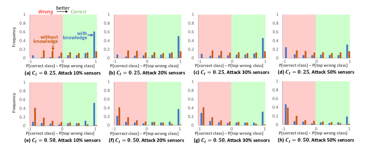
Figure 5: (PrimateNet) Histogram of the robustness margin (difference between the probability of the correct class (lower bound) and the top wrong class (upper bound)) under perturbation. If such a difference is positive, it means that the classifier makes the right prediction under perturbation. Evaluation is made under smoothing parameter $\sigma=0.25$ with $\ell_{2}$ perturbation scale $C_{I}=\{\sigma,2\sigma\}$. The ratio of the attacked sensors $\alpha$ equals to $10\%,20\%,30\%,50\%$.

From Figure 5, we can see that under different adversary scenarios, more instances could receive the positive margin (i.e correct prediction) with sensing-reasoning pipeline, which indicates its robustness. Moreover, we find that the sensing-reasoning pipeline could output a large margin value with high frequency under various attacks. That means, it can certify the robustness of the ground truth class with high confidence, which is challenging for current certified robustness approaches for single ML models.

In addition, to evaluate the utility of different knowledge, we also develop sensing-reasoning pipeline by using only one type of knowledge (hierarchical or exclusive relationship only) and the results are shown in Appendix I. We observe that using partial knowledge, the robustness of sensing-reasoning pipeline would decrease compared with that using the full knowledge.

Appendix G Image Classification on Word50 Dataset

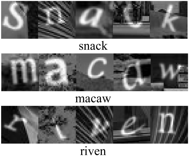
Figure 6: Several word images sampled from Word50 dataset.

Task and Dataset. In addition, we also conduct experiments on Word50 dataset [6], which is created by randomly selecting 50 words and each consisting of five characters. Here we only pick 10 words from it to reduce the computation complexity, and the goal is to classify these 10 words. All the character images are of size $28\times 28$ and perturbed by scaling, rotation, and translation. The background of the characters is blurry by inserting different patches, which makes it a quite challenging task. For reference, Some word images sampled from the dataset are shown in Figure 6. The interesting property of this dataset is that the character combination is given as the prior knowledge, which can be integrated into our sensing-reasoning pipeline. The training, validation, and test sets contain $2,049$, $408$, and $423$ variations of word styles respectively.

Similar to the classification task on Road Sign dataset, we develop the following two types of knowledge rules as follows:

• Deduction rules $(u,v_{i})$: word $u$ contains character $v_{i}$ on the $i$th position of the word.

• Exclusion rules $(u_{i},v_{i})$: character $u_{i}$ and character $v_{i}$ are naturally exclusive on the $i$th position of the word.

Implementation details. Multi-layer perceptrons (MLPs) are used as the main model architecture for the main task that the classification of the 10 words, which is the same to [6], and the input is the concatenation of the images of 5 characters which consist of a full word. As for the extra knowledge, we train another five MLP models for the classification of the character on each position of the input word, then the corresponding output dimensions for each such character classifier is $26$. While during the inference, we will only pick the top2 of the output from each character classifier, so the final input dimension to the MLN is $10+5\times 2=20$ dimensions. Thus, to keep the certification probability the same as the baseline, the $\zeta_{0}$ here will be set to $1-(1-0.001)^{(1/20)}=5.002\times 10^{-5}$.

For these sensing models, we adapt the randomized smoothing strategy [8] to give the certified robustness guarantee of their output confidence under the $\ell_{2}$-norm bounded perturbation. The $w_{H}$ is set to $2$ for the deduction rules, and the corresponding $f_{H}$ is the identity function; while for the exclusion rules, the $w_{H}$ is set to $-\infty$, and the $f_{H}$ here is the negation function, namely, $f_{H}(v)=1-v$.

Knowledge. We construct our first-order logical rules based on our predefined Deduction and Exclusion knowledge rules:

• Deduction edge $u\implies v_{i}$:

  $$x_{u}\wedge\neg x_{v_{i}}=\texttt{False}$$ (41)

• Exclusion edge $u_{i}\oplus v_{i}$:

  $$x_{u_{i}}\land x_{v_{i}}=\texttt{False}$$ (42)

Threat Model. Same to the setting of the experiments on the Stop Sign dataset, here we consider a stronger attack scenario where the attacker can attack the main task model and all the attribute sensors with different $\ell_{2}$-norm bounded perturbation $\delta:||\delta||_{2}<C_{I}$ at the same time. Later on, we can see our sensing-reasoning pipeline could still achieve higher end-to-end certified robustness under even harder cases.

Given the $\ell_{2}$-norm bound $C_{I}$, for each sensing model, we can bound its output probability $p^{\prime}$ under such perturbation, given the original probability $p$ and the certification smoothing parameter $\sigma$ according to Corollary 2 as below:

$$p^{\prime}\in[\Phi(\Phi^{-1}(p)-C_{I}/\sigma),\Phi(\Phi^{-1}(p)+C_{I}/\sigma)].$$

Evaluation Metrics. We adopt the standard certified accuracy as our evaluation metric, defined by the percentage of instances that can be certified under any $\ell_{2}$-norm bounded perturbation $\delta:||\delta||_{2}<C_{I}$. Specifically, given the input $x$ with ground-truth label $y$, we can certify the bound of confidence on predicting label $y$ as $[\mathcal{L},\mathcal{U}]$ for either a vanilla randomize smoothing-based model or our sensing-reasoning pipeline. After that, the certified accuracy can be defined by: $\frac{1}{N}\sum_{i=1}^{N}\mathbbm{I}([\mathcal{L}_{i}>0.5])$ where $\mathbbm{I}(\cdot)$ denotes the indicator function.

Intuitive Example. To make the example more clear, here we use pos(’a’, i) to represent that the character ’a’ is in the ith position of the word. Then during the inference, given an input word image, we assume the top2 characters returned from the character classifiers for each position is ’s,m’, ’n,b’, ’a,o’, ’q,a’, ’k,c’, which are shown in the order of the position. Now, for word ’snack’, the corresponding first-order logical form of its deduction rules would be $\emph{'snack'}\implies$ pos(’s’, $1$), $\emph{'snack'}\implies$ pos(’n’, $2$), $\emph{'snack'}\implies$ pos(’a’, $3$) and $\emph{'snack'}\implies$ pos(’k’, $5$); while for other words like ’macaw’, the corresponding rules would be $\emph{'macaw'}\implies$ pos(’m’, $1$) and $\emph{'macaw'}\implies$ pos(’a’, $4$). Notice, if the character of the specific word is not shown in the top2 returned characters of its corresponding position, then there will be no deduction rule built for this word and this character. At the meantime, when we consider the possible worlds that satisfy $\sigma(x_{\emph{snack}})\land\sigma(v_{\emph{pos}(\emph{'q'},4})=1$, we will still consider it as a violation of the exclusive rules. In other words, even if the character ’c’ is not shown in the top2 characters returned from the knowledge classifier in fourth position and thus we do not build the deduction rule $\emph{'snack'}\implies$ pos(’c’, $4$) explicitly at this time as said above, this rule is still assumed to be true underlyingly.

Evaluation Results. We evaluate the robustness of the sensing-reasoning pipeline and compare it to the baseline as a vanilla randomized smoothed main task model (without knowledge). We train our models under different smoothing parameters $\hat{\sigma}=\{0.12,0.25,0.50\}$ and evaluate our sensing-reasoning pipeline under various $\ell_{2}$ perturbation magnitude $C_{I}=\{0.12,0.25,0.50,1.00\}$. Results are show in Table 5, and as we can see, with extra knowledge, the performance is improved tremendously which strongly demonstrates the potential of the sensing-reasoning pipeline.

Table 5: Certified accuracy under different perturbation magnitude $C_{I}$ on Word10 dataset. The sensing models are smoothed with Gaussian noise $\epsilon\sim\mathcal{N}(0,\hat{\sigma}^{2}I_{d})$ with different smoothing parameter $\hat{\sigma}$. Rows with $\ast$ denote the best certified accuracy among all the $\hat{\sigma}\in\{0.12,0.25,0.50\}$. (All certificates holds with 99.9% confidence)

Methods	$\sigma$	$C_{I}=0.12$	$C_{I}=0.25$	$C_{I}=0.50$	$C_{I}=1.00$
	0.12	58.2	49.2	0.0	0.0
Vanilla Smoothing	0.25	51.8	42.3	25.3	0.0
(w/o knowledge)	0.50	42.6	33.1	19.1	2.6
	$\ast$	58.2	49.2	25.3	2.6
	0.12	88.7	77.8	30.7	0.0
Sensing-Reasoning Pipeline	0.25	95.0	90.8	52.5	2.8
(w/ knowledge)	0.50	91.5	86.8	69.3	6.4
	$\ast$	95.0	90.8	69.3	6.4

Appendix H Image Classification with Constructed Knowledge Rules

For natural image datasets with no apparent knowledge rules, we can still apply our sensing-reasoning pipeline based on some generated simple knowledge rules such as redundancy rules. For instance, we test on MNIST and CIFAR10 dataset by constructing basic rules as follows: for MNIST, we construct five pseudo attributes and randomly assign them to four different digits, so that each digit will exactly contain two pseudo attributes; for CIFAR10, we randomly generate ten pseudo attributes, and each pseudo attribute will be randomly assigned to 3 to 7 different categories. We build the indication rules between each pseudo attribute and its corresponding digits, and the exclusion rules between different digit classes.

During the training, we adopt the SOTA Consistency training [19] as our sensing model training method, and build our sensing-reasoning pipeline on top of these pretrained sensing models.

From the results shown in Table 6 and Table 7, we can see that the sensing-reasoning pipeline beats the SOTA baselines in terms of the certified robustness even with the simple and generated knowledge rules. Generally, we should expect higher certified robustness by integrating with natural and meaningful knowledge rules (e.g., road sign classification and information extraction tasks as shown in our paper).

Table 6: (MNIST) Certified accuracy under different input perturbation magnitudes ($C_{I}$).

Methods	$C_{I}=0.00$	$C_{I}=0.25$	$C_{I}=0.50$	$C_{I}=0.75$	$C_{I}=1.00$	$C_{I}=1.25$	$C_{I}=1.50$	$C_{I}=1.75$	$C_{I}=2.00$
Consistency Training	99.5	98.9	98.0	96.0	93.0	87.8	78.5	60.5	41.7
Sensing-Reasoning Pipeline (Consistency)	99.6	98.2	97.6	96.3	93.5	88.2	78.9	61.2	43.2

Table 7: (CIFAR10) Certified accuracy under different input perturbation magnitudes ($C_{I}$).

Methods	$C_{I}=0.00$	$C_{I}=0.25$	$C_{I}=0.50$	$C_{I}=0.75$	$C_{I}=1.00$	$C_{I}=1.25$	$C_{I}=1.50$	$C_{I}=1.75$	$C_{I}=2.00$
Consistency Training	77.8	68.8	57.4	43.8	36.2	29.5	22.9	19.7	16.6
Sensing-Reasoning Pipeline (Consistency)	78.4	70.4	56.2	46.0	37.4	29.6	25.2	21.8	18.8

Appendix I Ablation Study on Partial Knowledge Enrichment.

In PrimateNet experiments, we also investigate how Hierarchy knowledge and Exclusive knowledge would affect the End-to-end robustness of our sensing-reasoning pipeline individually. We compare the certified robustness and certified ratio of our sensing-reasoning pipeline enriched by {No knowledge; Hierarchy knowledge only; Exclusive knowledge only; Hierarchy + Exclusive knowledge} and the results are shown in Table I and I.

From the results, we can see while partial knowledge enrichment would lead to fragile robustness under severe scenarios ($\alpha=0.5$), complete knowledge enrichment could achieve much better robustness compared to sensing-reasoning pipeline without knowledge enrichment. This indicates that incomplete (or weak) knowledge, which is easy to break and hard to recover under severe adversarial scenarios, could even harm the robustness of our sensing-reasoning pipeline. How to explore good and robust knowledge to enrich our sensing-reasoning pipeline could be our interesting future direction.

Table 8: Certified Robustness with different perturbation magnitude $C_{I}$ and sensing model attack ratio $\alpha$ on PrimateNet. The sensing models are smoothed with Gaussian noise $\epsilon\sim\mathcal{N}(0,\hat{\sigma}^{2}I_{d})$ with different smoothing parameter $\sigma$. Here “Hierarchy.” refers to the sensing-reasoning pipeline enriched by hierarchy knowledge only while “Exclusive.” the exclusive knowledge only. “Combined.” shows the sensing-reasoning pipeline enriched by both domain knowledge.

(a) $\hat{\sigma}=0.12$

$C_{I}$	$\alpha$	No knowledge	Hierarchy.	Exclusive.	Combined.
0.12	10%	0.5724	0.7912	0.7020	0.8849
	20%	0.5717	0.6932	0.6236	0.8078
	30%	0.5706	0.6280	0.5624	0.7508
	50%	0.5706	0.4868	0.4320	0.6236
0.25	10%	0.2342	0.6670	0.5232	0.7888
	20%	0.2320	0.4704	0.3468	0.6226
	30%	0.2309	0.3632	0.3158	0.5225
	50%	0.2268	0.2122	0.2004	0.3594

$C_{I}$	$\alpha$	No knowledge	Hierarchy.	Exclusive.	Combined.
0.25	10%	0.5314	0.7766	0.6998	0.8498
	20%	0.5302	0.6810	0.6002	0.7608
	30%	0.5294	0.6278	0.5464	0.7217
	50%	0.5235	0.4924	0.4126	0.6026
0.50	10%	0.2024	0.6754	0.5196	0.7622
	20%	0.2024	0.4636	0.3298	0.5988
	30%	0.2010	0.3680	0.2870	0.5324
	50%	0.2000	0.2204	0.1652	0.3417

(c) $\hat{\sigma}=0.50$ $C_{I}$ $\alpha$ No knowledge Hierarchy. Exclusive. Combined. 0.50 10% 0.4762 0.7412 0.6952 0.8288 20% 0.4749 0.6120 0.5884 0.7407 30% 0.4736 0.5410 0.5002 0.6907 50% 0.4635 0.4040 0.3862 0.5581 1.00 10% 0.1679 0.6000 0.4838 0.7307 20% 0.1615 0.3834 0.3184 0.5285 30% 0.1612 0.2920 0.2362 0.4347 50% 0.1584 0.1498 0.1404 0.2624

Table 9: Certified Ratio with different perturbation magnitude $C_{I}$ and sensing model attack ratio $\alpha$ on PrimateNet. The sensing models are smoothed with Gaussian noise $\epsilon\sim\mathcal{N}(0,\hat{\sigma}^{2}I_{d})$ with different smoothing parameter $\sigma$. Here “Hierarchy.” refers to the sensing-reasoning pipeline enriched by hierarchy knowledge only while “Exclusive.” the exclusive knowledge only. “Combined.” shows the sensing-reasoning pipeline enriched by both domain knowledge.

(a) $\hat{\sigma}=0.12$

$C_{I}$	$\alpha$	No knowledge	Hierarchy.	Exclusive.	Combined.
0.12	10%	0.5724	0.8714	0.7320	0.9419
	20%	0.5717	0.7586	0.6442	0.8609
	30%	0.5706	0.6850	0.5928	0.7988
	50%	0.5706	0.5270	0.4642	0.6647
0.25	10%	0.2342	0.7330	0.5482	0.8428
	20%	0.2320	0.5150	0.3842	0.6657
	30%	0.2309	0.4011	0.3422	0.5596
	50%	0.2268	0.2322	0.2262	0.3824

$C_{I}$	$\alpha$	No knowledge	Hierarchy.	Exclusive.	Combined.
0.25	10%	0.5314	0.9102	0.7254	0.9499
	20%	0.5302	0.7910	0.6226	0.8952
	30%	0.5294	0.7322	0.5878	0.8048
	50%	0.5235	0.5670	0.4302	0.6747
0.50	10%	0.2024	0.7998	0.5322	0.8489
	20%	0.2024	0.5512	0.3490	0.6467
	30%	0.2010	0.4440	0.3266	0.5541
	50%	0.2000	0.2632	0.1734	0.3635

(c) $\hat{\sigma}=0.50$ $C_{I}$ $\alpha$ No knowledge Hierarchy. Exclusive. Combined. 0.50 10% 0.4762 0.8924 0.7128 0.9449 20% 0.4749 0.7370 0.6144 0.8488 30% 0.4736 0.6552 0.5462 0.7968 50% 0.4635 0.4938 0.4324 0.6395 1.00 10% 0.1679 0.7374 0.5204 0.8448 20% 0.1615 0.4906 0.3398 0.6336 30% 0.1612 0.3850 0.2926 0.5375 50% 0.1584 0.1996 0.1628 0.3318

Appendix J Reasoning Component as Bayesian Networks

A Bayesian network (BN) is a probabilistic graphical model that represents a set of variables and their conditional dependencies with a directed acyclic graph. Let us first consider a Bayesian Network with tree structures, the probability of a random variable being 1 is given by

$$\mathbf{Pr}\left[X=1,\{p_{i}\}\right]=\sum_{x_{1},...x_{n}}P(1|x_{1},...,x_{n})\prod_{i}p_{i}^{x_{i}}(1-p_{i})^{1-x_{i}}$$

In the following subsections, we will prove a hardness result of checking robustness in general MLN and BNs and use the above definition to construct an efficient procedure to certify robustness for binary tree BNs.

J.1 Hardness of Certifying Bayesian Networks

Analogously with the above reasoning, we can also state the general hardness result for deciding the robustness of BNs:

Theorem 3 (BN hardness).

Given a Bayesian network with a set of parameters $\{p_{i}\}$, a set of perturbation parameters $\{\epsilon_{i}\}$ and threshold $\delta$, deciding whether

$$|\mathbf{Pr}\left[X=1;\{p_{i}\}\right]-\mathbf{Pr}\left[X=1;\{p_{i}+\epsilon_{i}\}\right]|<\delta$$

is at least as hard as estimating $\mathbf{Pr}\left[X=1;\{p_{i}\}\right]$ up to $\varepsilon_{c}$ multiplicative error, with $\epsilon_{i}=O(\varepsilon_{c})$.

Proof.

Let $\alpha=[p_{i}]$, $Q(\sigma)=X$ and $\pi_{\alpha}$ defined by the the probability distribution of a target random variable. Since $X\in\{0,1\}$, we have $\mathbb{E}[\sigma\sim\pi_{\alpha}]{Q(\sigma)}=\mathbf{Pr}\left[X=1;\{p_{i}\}\right]$. The proof then follows analogously from Theorem 1. ∎

Based on the hardness analysis of the reasoning robustness, we can see that it is challenging to directly certify the robustness of the reasoning component. However, just as we can approximately certify the robustness of single ML models [25], in the next section, we will present and discuss how to approximately certify the robustness of the reasoning component, and we show that for some structures such as BN trees, the certification could even be tight.

J.2 Certifying Bayesian Networks

Apart from MLNs, we also aim to reason about the robustness for Bayesian networks with binary tree structures, and derive an efficient algorithm to provide the tight upper and lower bounds of reasoning robustness. Concretely, we introduce the set of perturbation $\{\epsilon_{i}\}$ on $\{p_{i}\}$ and consider the maximum resultant probability:

$$\max_{\epsilon_{1}...\epsilon_{n}}\sum_{x_{1},...x_{n}}P(1|x_{1},...,x_{n})\prod_{i}(p_{i}+\epsilon_{i})^{x_{i}}(1-p_{i}-\epsilon_{i})^{1-x_{i}}$$

$$= \max_{\epsilon_{1}...\epsilon_{n}}\sum_{x_{1},...x_{n-1}}\Bigg{(}\prod_{i<n}(p_{i}+\epsilon_{i})^{x_{i}}(1-p_{i}-\epsilon_{i})^{1-x_{i}}\Bigg{)}\times$$

$$~{}~{}~{}~{}~{}~{}~{}~{}~{}~{}~{}~{}~{}~{}~{}~{}~{}~{}~{}~{}\Bigg{(}P(1|x_{1},...,x_{n-1},0)(1-p_{n}-\epsilon_{n})+P(1|x_{1},...,x_{n-1},1)(p_{n}+\epsilon_{n})\Bigg{)}$$

$$= \max_{\epsilon_{1}...\epsilon_{n}}\sum_{x_{1},...x_{n-1}}\left(\prod_{i<n}(p_{i}+\epsilon_{i})^{x_{i}}(1-p_{i}-\epsilon_{i})^{1-x_{i}}\right)\times$$

$$~{}~{}~{}~{}~{}~{}~{}~{}~{}~{}~{}~{}~{}~{}~{}~{}~{}~{}~{}~{}\Bigg{(}P(1|x_{1},...,x_{n-1},0)+\Big{(}P(1|x_{1},...,x_{n-1},1)-P(1|x_{1},...,x_{n-1},0)\Big{)}(p_{n}+\epsilon_{n})\Bigg{)}.$$

In the above we have isolated the last variable in the expression. Without additional structure, the above optimisation over perturbation is hard as stated in Theorem 3. However, if additionally we require the Bayesian network to be binary trees, we show that the optimisation over perturbation and the checking of robustness of the model is trackable. We summarise the procedure for checking robustness of binary tree structured BNs in the following theorem with the proof.

Lemma J.1 (Binary BN Robustness).

Given a Bayesian network with binary tree structure, and the set of parameters $\{p_{i}\}$, the probability of a variable $X=1$,

$$\mathbf{Pr}\left[X=1,\{p_{i}\}\right]=\sum_{x_{1},x_{2}}P(1|x_{1},x_{2})\prod_{i}p_{i}^{x_{i}}(1-p_{i})$$

is $\delta_{b}$-robust, where

$$\delta_{b} =\max\bigg{\{}\Big{|}\mathbf{Pr}\left[X=1,\{p_{i}\}\right]-F_{max}\Big{|},\Big{|}\mathbf{Pr}\left[X=1,\{p_{i}\}\right]-F_{min}\Big{|}\bigg{\}}$$

$$with~{}~{}~{}~{}~{}~{} F_{max}=\max_{y_{1},y_{2}}A_{0}+A_{1}(y_{1}+y_{2})+(A_{2}-A_{1})y_{1}y_{2},$$

$$F_{min}=\min_{y_{1},y_{2}}A_{0}+A_{1}(y_{1}+y_{2})+(A_{2}-A_{1})y_{1}y_{2},~{}~{}~{}~{}$$

$$s.t.,y_{i}\in[p_{i}-C_{i},p_{i}+C_{i}],$$

Where $A_{0}=P(1|0,0)$, $A_{1}=P(1|0,1)-P(1|0,0)$ and $A_{2}=P(1|1,1)-P(1|0,1)$ are all pre-computable constants given the parameters of the Bayesian network.

Proof of Lemma J.1

Proof.

We explicitly write out the probability subject to perturbation,

$$\mathbf{Pr}\left[X=1,\{p_{i}+\epsilon_{i}\}$$

$$= \sum_{x_{1},x_{2}}P(1|x_{1},x_{2})\prod_{i}(p_{i}+\epsilon_{i})^{x_{i}}(1-p_{i}-\epsilon_{i})^{1-x_{i}}$$

$$= (p_{1}+\epsilon_{1})\sum_{x_{2}}P(1|1,x_{2})(p_{2}+\epsilon_{2})^{x_{2}}(1-p_{2}-\epsilon_{2})^{1-x_{2}}$$

$$+(1-p_{1}-\epsilon_{1})\sum_{x_{2}}P(1|0,x_{2})(p_{2}+\epsilon_{2})^{x_{2}}(1-p_{2}-\epsilon_{2})^{1-x_{2}}$$

$$= \sum_{x_{2}}P(1|0,x_{2})(p_{2}+\epsilon_{2})^{x_{2}}(1-p_{2}-\epsilon_{2})^{1-x_{2}}$$

$$+(p_{1}+\epsilon_{1})\left(\sum_{x_{2}}\Big{(}P(1|1,x_{2})-P(1|0,x_{2})\Big{)}(p_{2}+\epsilon_{2})^{x_{2}}(1-p_{2}-\epsilon_{2})^{1-x_{2}}\right)$$

$$= \sum_{x_{2}}P(1|0,x_{2})(p_{2}+\epsilon_{2})^{x_{2}}(1-p_{2}-\epsilon_{2})^{1-x_{2}}$$

$$+(p_{1}+\epsilon_{1})\bigg{(}\Big{(}P(1|1,1)-P(1|0,1)\Big{)}(p_{2}+\epsilon_{2})+\Big{(}P(1|1,0)-P(1|0,0)\Big{)}(1-p_{2}-\epsilon_{2})\bigg{)}$$

$$= P(1|0,0)+\Big{(}P(1|0,1)-P(1|0,0)\Big{)}(p_{2}+\epsilon_{2})+(p_{1}+\epsilon_{1})\times$$

$$\bigg{(}P(1|1,0)-P(1|0,0)+\Big{(}P(1|1,1)-P(1|0,1)-P(1|1,0)+P(1|0,0)\Big{)}(p_{2}+\epsilon_{2})\bigg{)}.$$

It follows that the robustness problem boils down to finding the maximum and minimum of $F=A_{0}+A_{1}y_{2}+A_{1}y_{1}+(A_{2}-A_{1})y_{1}y_{2}$, with $y_{i}=p_{i}+\epsilon_{i}$. ∎

Specifically, in order to compute $F_{max}$ and $F_{min}$, we take partial derivatives of F:

$$\frac{\partial F}{\partial y_{1}}=A_{1}+(A_{2}-A_{1})y_{2},$$

$$\frac{\partial F}{\partial y_{2}}=A_{1}+(A_{2}-A_{1})y_{1}.$$

Setting $\frac{\partial F}{\partial y_{1}}=\frac{\partial F}{\partial y_{2}}=0$ leads to $y_{1}^{*}=y_{2}^{*}=\frac{A_{1}}{A_{1}-A_{2}}$. In order to check if $y_{i}^{*}$ correspond to maximum or minimum. evaluate $\frac{\partial^{2}F}{\partial y_{i}^{2}}=A_{2}-A_{1}$. We have the following scenarios:

• If $y_{i}^{*}\in[p_{i}-C_{i},p_{i}+C_{i}]$ and $A_{2}-A_{1}>0$, then $y_{i}^{*}$ correspond to a minimum.

• If $y_{i}^{*}\in[p_{i}-C_{i},p_{i}+C_{i}]$ and $A_{2}-A_{1}<0$, then $y_{i}^{*}$ correspond to a maximum.

• If $y_{i}^{*}\notin[p_{i}-C_{i},p_{i}+C_{i}]$, then $y_{i}$ is monotonic in the range of $[p_{i}-C_{i},p_{i}+C_{i}]$ and the maximum or minimum are found at $p_{i}\pm C_{i}$.

Having shown the robustness of probability of one node in the Bayesian network, the robustness of the whole network can be computed recursively from the bottom to the top.

References

- [1] Anish Athalye, Nicholas Carlini, and David Wagner. Obfuscated gradients give a false sense of security: Circumventing defenses to adversarial examples. In International Conference on Machine Learning, pages 274–283, 2018.
- [2] Marenglen Biba, Stefano Ferilli, and Floriana Esposito. Protein fold recognition using markov logic networks. In Mathematical Approaches to Polymer Sequence Analysis and Related Problems, pages 69–85. Springer, 2011.
- [3] Nicholas Carlini and David Wagner. Towards evaluating the robustness of neural networks. In 2017 ieee symposium on security and privacy (sp), pages 39–57. IEEE, 2017.
- [4] Yair Carmon, Aditi Raghunathan, Ludwig Schmidt, Percy Liang, and John C Duchi. Unlabeled data improves adversarial robustness. arXiv preprint arXiv:1905.13736, 2019.
- [5] Deepayan Chakrabarti, Stanislav Funiak, Jonathan Chang, and Sofus A Macskassy. Joint inference of multiple label types in large networks. arXiv preprint arXiv:1401.7709, 2014.
- [6] Liang-Chieh Chen, Alexander Schwing, Alan Yuille, and Raquel Urtasun. Learning deep structured models. In International Conference on Machine Learning, pages 1785–1794. PMLR, 2015.
- [7] Liwei Chen, Yansong Feng, Jinghui Mo, Songfang Huang, and Dongyan Zhao. Joint inference for knowledge base population. In Proceedings of the 2014 Conference on Empirical Methods in Natural Language Processing (EMNLP), pages 1912–1923, Doha, Qatar, October 2014. Association for Computational Linguistics.
- [8] Jeremy M Cohen, Elan Rosenfeld, and J Zico Kolter. Certified adversarial robustness via randomized smoothing. arXiv preprint arXiv:1902.02918, 2019.
- [9] J. Deng, W. Dong, R. Socher, L.-J. Li, K. Li, and L. Fei-Fei. ImageNet: A Large-Scale Hierarchical Image Database. In CVPR09, 2009.
- [10] Jia Deng, Nan Ding, Yangqing Jia, Andrea Frome, Kevin Murphy, Samy Bengio, Yuan Li, Hartmut Neven, and Hartwig Adam. Large-scale object classification using label relation graphs. In European conference on computer vision, pages 48–64. Springer, 2014.
- [11] Jacob Devlin, Ming-Wei Chang, Kenton Lee, and Kristina Toutanova. BERT: pre-training of deep bidirectional transformers for language understanding. In Jill Burstein, Christy Doran, and Thamar Solorio, editors, NAACL-HLT, pages 4171–4186. Association for Computational Linguistics, 2019.
- [12] Xiao Ding, Yue Zhang, Ting Liu, and Junwen Duan. Using structured events to predict stock price movement: An empirical investigation. In Proceedings of the 2014 Conference on Empirical Methods in Natural Language Processing (EMNLP), pages 1415–1425, 2014.
- [13] Kevin Eykholt, Ivan Evtimov, Earlence Fernandes, Bo Li, Amir Rahmati, Chaowei Xiao, Atul Prakash, Tadayoshi Kohno, and Dawn Song. Robust physical-world attacks on deep learning visual classification. In Proceedings of the IEEE Conference on Computer Vision and Pattern Recognition, pages 1625–1634, 2018.
- [14] Christiane Fellbaum. Wordnet. The encyclopedia of applied linguistics, 2012.
- [15] Ian J. Goodfellow, Jonathon Shlens, and Christian Szegedy. Explaining and harnessing adversarial examples. ICLR, 2015.
- [16] Sven Gowal, Krishnamurthy Dvijotham, Robert Stanforth, Rudy Bunel, Chongli Qin, Jonathan Uesato, Relja Arandjelovic, Timothy Mann, and Pushmeet Kohli. On the effectiveness of interval bound propagation for training verifiably robust models. arXiv preprint arXiv:1810.12715, 2018.
- [17] Nezihe Merve Gürel, Xiangyu Qi, Luka Rimanic, Ce Zhang, and Bo Li. Knowledge enhanced machine learning pipeline against diverse adversarial attacks. ICML, 2021.
- [18] Tuyen N Huynh and Raymond J Mooney. Max-margin weight learning for markov logic networks. In Joint European Conference on Machine Learning and Knowledge Discovery in Databases, pages 564–579. Springer, 2009.
- [19] Jongheon Jeong and Jinwoo Shin. Consistency regularization for certified robustness of smoothed classifiers. Advances in Neural Information Processing Systems, 33:10558–10570, 2020.
- [20] J Zico Kolter and Eric Wong. Provable defenses against adversarial examples via the convex outer adversarial polytope. arXiv preprint arXiv:1711.00851, 2017.
- [21] Ondrej Kuzelka. Complex markov logic networks: Expressivity and liftability. In Conference on Uncertainty in Artificial Intelligence, pages 729–738. PMLR, 2020.
- [22] Bo Li and Yevgeniy Vorobeychik. Feature cross-substitution in adversarial classification. In Advances in neural information processing systems, pages 2087–2095, 2014.
- [23] Huichen Li, Linyi Li, Xiaojun Xu, Xiaolu Zhang, Shuang Yang, and Bo Li. Nonlinear gradient estimation for query efficient blackbox attack. In International Conference on Artificial Intelligence and Statistics (AISTATS 2021), Proceedings of Machine Learning Research. PMLR, 13–15 Apr 2021.
- [24] Huichen Li, Xiaojun Xu, Xiaolu Zhang, Shuang Yang, and Bo Li. Qeba: Query-efficient boundary-based blackbox attack. In Proceedings of the IEEE/CVF Conference on Computer Vision and Pattern Recognition, pages 1221–1230, 2020.
- [25] Linyi Li, Xiangyu Qi, Tao Xie, and Bo Li. Sok: Certified robustness for deep neural networks. arXiv, abs/2009.04131, 2020.
- [26] Linyi Li, Maurice Weber, Xiaojun Xu, Luka Rimanic, Bhavya Kailkhura, Tao Xie, Ce Zhang, and Bo Li. Tss: Transformation-specific smoothing for robustness certification. In ACM Conference on Computer and Communications Security (CCS 2021), 2021.
- [27] Linyi Li, Jiawei Zhang, Tao Xie, and Bo Li. Double sampling randomized smoothing. In International Conference on Machine Learning, 2022.
- [28] Linyi Li, Zexuan Zhong, Bo Li, and Tao Xie. Robustra: training provable robust neural networks over reference adversarial space. In Proceedings of the 28th International Joint Conference on Artificial Intelligence, pages 4711–4717. AAAI Press, 2019.
- [29] Daniel Lowd and Pedro Domingos. Efficient weight learning for markov logic networks. In Joost N. Kok, Jacek Koronacki, Ramon Lopez de Mantaras, Stan Matwin, Dunja Mladenič, and Andrzej Skowron, editors, Knowledge Discovery in Databases: PKDD 2007, pages 200–211, Berlin, Heidelberg, 2007. Springer Berlin Heidelberg.
- [30] Xingjun Ma, Bo Li, Yisen Wang, Sarah M Erfani, Sudanthi Wijewickrema, Grant Schoenebeck, Dawn Song, Michael E Houle, and James Bailey. Characterizing adversarial subspaces using local intrinsic dimensionality. arXiv preprint arXiv:1801.02613, 2018.
- [31] Aleksander Madry, Aleksandar Makelov, Ludwig Schmidt, Dimitris Tsipras, and Adrian Vladu. Towards deep learning models resistant to adversarial attacks. arXiv preprint arXiv:1706.06083, 2017.
- [32] Emily K. Mallory, Ce Zhang, Christopher Ré, and Russ B. Altman. Large-scale extraction of gene interactions from full-text literature using DeepDive. Bioinformatics, 32(1):106–113, 09 2015.
- [33] Andrew McCallum. Joint inference for natural language processing. In Proceedings of the Thirteenth Conference on Computational Natural Language Learning (CoNLL-2009), page 1, Boulder, Colorado, June 2009. Association for Computational Linguistics.
- [34] Tianyu Pang, Kun Xu, Chao Du, Ning Chen, and Jun Zhu. Improving adversarial robustness via promoting ensemble diversity. arXiv preprint arXiv:1901.08846, 2019.
- [35] Judea Pearl. Causality: Models, Reasoning, and Inference. Cambridge University Press, USA, 2000.
- [36] Judea Pearl. Bayesian networks. 2011.
- [37] Shanan E. Peters, Ce Zhang, Miron Livny, and Christopher Ré. A machine reading system for assembling synthetic paleontological databases. PLOS ONE, 9(12):1–22, 12 2014.
- [38] Hoifung Poon and Pedro Domingos. Joint inference in information extraction. In AAAI, volume 7, pages 913–918, 2007.
- [39] Haonan Qiu, Chaowei Xiao, Lei Yang, Xinchen Yan, Honglak Lee, and Bo Li. Semanticadv: Generating adversarial examples via attribute-conditioned image editing. In European Conference on Computer Vision, pages 19–37. Springer, 2020.
- [40] Matthew Richardson and Pedro Domingos. Markov logic networks. Machine learning, 62(1-2):107–136, 2006.
- [41] Matthew Richardson and Pedro Domingos. Markov logic networks. Machine Learning, 62(1-2):107–136, 2006.
- [42] Hadi Salman, Jerry Li, Ilya Razenshteyn, Pengchuan Zhang, Huan Zhang, Sebastien Bubeck, and Greg Yang. Provably robust deep learning via adversarially trained smoothed classifiers. In Advances in Neural Information Processing Systems, pages 11289–11300, 2019.
- [43] Shibani Santurkar, Dimitris Tsipras, Mahalaxmi Elango, David Bau, Antonio Torralba, and Aleksander Madry. Editing a classifier by rewriting its prediction rules. Advances in Neural Information Processing Systems, 34:23359–23373, 2021.
- [44] Ali Shafahi, Mahyar Najibi, Amin Ghiasi, Zheng Xu, John Dickerson, Christoph Studer, Larry S Davis, Gavin Taylor, and Tom Goldstein. Adversarial training for free! arXiv preprint arXiv:1904.12843, 2019.
- [45] Johannes Stallkamp, Marc Schlipsing, Jan Salmen, and Christian Igel. Man vs. computer: Benchmarking machine learning algorithms for traffic sign recognition. Neural networks, 32:323–332, 2012.
- [46] Vincent Tjeng, Kai Xiao, and Russ Tedrake. Evaluating robustness of neural networks with mixed integer programming. arXiv preprint arXiv:1711.07356, 2017.
- [47] Florian Tramer, Nicholas Carlini, Wieland Brendel, and Aleksander Madry. On adaptive attacks to adversarial example defenses. arXiv preprint arXiv:2002.08347, 2020.
- [48] Florian Tramèr, Alexey Kurakin, Nicolas Papernot, Dan Boneh, and Patrick McDaniel. Ensemble adversarial training: Attacks and defenses. ICLR, 2018.
- [49] Dimitris Tsipras, Shibani Santurkar, Logan Engstrom, Alexander Turner, and Aleksander Madry. Robustness may be at odds with accuracy). ICLR 2019, 2018.
- [50] L.G. Valiant. The complexity of computing the permanent. Theoretical Computer Science, 8(2):189–201, 1979.
- [51] Martin J. Wainwright and Michael I. Jordan. Graphical models, exponential families, and variational inference. Foundations and Trends® in Machine Learning, 1(1–2):1–305, 2008.
- [52] Lily Weng, Huan Zhang, Hongge Chen, Zhao Song, Cho-Jui Hsieh, Luca Daniel, Duane Boning, and Inderjit Dhillon. Towards fast computation of certified robustness for relu networks. In International Conference on Machine Learning, pages 5276–5285, 2018.
- [53] Chaowei Xiao, Ruizhi Deng, Bo Li, Taesung Lee, Benjamin Edwards, Jinfeng Yi, Dawn Song, Mingyan Liu, and Ian Molloy. Advit: Adversarial frames identifier based on temporal consistency in videos. In Proceedings of the IEEE/CVF International Conference on Computer Vision, pages 3968–3977, 2019.
- [54] Chaowei Xiao, Ruizhi Deng, Bo Li, Fisher Yu, Mingyan Liu, and Dawn Song. Characterizing adversarial examples based on spatial consistency information for semantic segmentation. In Proceedings of the European Conference on Computer Vision (ECCV), pages 217–234, 2018.
- [55] Kaidi Xu, Zhouxing Shi, Huan Zhang, Yihan Wang, Kai-Wei Chang, Minlie Huang, Bhavya Kailkhura, Xue Lin, and Cho-Jui Hsieh. Automatic perturbation analysis for scalable certified robustness and beyond. Advances in Neural Information Processing Systems, 33, 2020.
- [56] Zhe Xu, Ivan Gavran, Yousef Ahmad, Rupak Majumdar, Daniel Neider, Ufuk Topcu, and Bo Wu. Joint inference of reward machines and policies for reinforcement learning. arXiv preprint arXiv:1909.05912, 2019.
- [57] Greg Yang, Tony Duan, J Edward Hu, Hadi Salman, Ilya Razenshteyn, and Jerry Li. Randomized smoothing of all shapes and sizes. In International Conference on Machine Learning, pages 10693–10705. PMLR, 2020.
- [58] Zhuolin Yang, Linyi Li, Xiaojun Xu, Bhavya Kailkhura, Tao Xie, and Bo Li. On the certified robustness for ensemble models and beyond. ICLR, 2021.
- [59] Zhuolin Yang, Linyi Li, Xiaojun Xu, Bhavya Kailkhura, Tao Xie, and Bo Li. On the certified robustness for ensemble models and beyond. In International Conference on Learning Representations, 2022.
- [60] Zhuolin Yang, Linyi Li, Xiaojun Xu, Shiliang Zuo, Qian Chen, Pan Zhou, Benjamin I. P. Rubinstein, Ce Zhang, and Bo Li. Trs: Transferability reduced ensemble via promoting gradient diversity and model smoothness. In Neural Information Processing Systems (NeurIPS 2021), 2021.
- [61] Zhuolin Yang, Linyi Li, Xiaojun Xu, Shiliang Zuo, Qian Chen, Pan Zhou, Benjamin I P Rubinstein, Ce Zhang, and Bo Li. Trs: Transferability reduced ensemble via promoting gradient diversity and model smoothness. In Advances in Neural Information Processing Systems, 2021.
- [62] Zhuolin Yang, Zhikuan Zhao, Boxin Wang, Jiawei Zhang, Linyi Li, Hengzhi Pei, Bojan Karlaš, Ji Liu, Heng Guo, Ce Zhang, and Bo Li. Improving certified robustness via statistical learning with logical reasoning. NeurIPS, 2022.
- [63] Ce Zhang, Christopher Ré, Michael Cafarella, Christopher De Sa, Alex Ratner, Jaeho Shin, Feiran Wang, and Sen Wu. Deepdive: Declarative knowledge base construction. Commun. ACM, 60(5):93–102, April 2017.
- [64] Huan Zhang, Tsui-Wei Weng, Pin-Yu Chen, Cho-Jui Hsieh, and Luca Daniel. Efficient neural network robustness certification with general activation functions. In Advances in neural information processing systems, pages 4939–4948, 2018.
- [65] Jiawei Zhang, Linyi Li, Huichen Li, Xiaolu Zhang, Shuang Yang, and Bo Li. Progressive-scale boundary blackbox attack via projective gradient estimation. ICML, 2022.