Simultaneous confidence bands for nonparametric regression

with partially missing covariates

Li Cai¹, Lijie Gu² , Qihua Wang¹, and Suojin Wang ³

¹Zhejiang Gongshang University, ²Soochow University, and ³Texas A&M University

Abstract: In this paper, we consider a weighted local linear estimator based on the inverse selection probability for nonparametric regression with missing covariates at random. The asymptotic distribution of the maximal deviation between the estimator and the true regression function is derived and an asymptotically accurate simultaneous confidence band is constructed. The estimator for the regression function is shown to be oracally efficient in the sense that it is uniformly indistinguishable from that when the selection probabilities are known. Finite sample performance is examined via simulation studies which support our asymptotic theory. The proposed method is demonstrated via an analysis of a data set from the Canada 2010/2011 Youth Student Survey.

Key words and phrases: Brownian motion, Maximal deviation, Simultaneous confidence band, Weighted local linear regression.

1. Introduction

In nonparametric data analysis, one important problem is to detect the global shape of unknown curves or to test whether these curves follow some specific functional forms that describe the overall trend of the regression relationship. Many researchers have attempted to solve this problem by constructing nonparametric simultaneous confidence bands (SCBs) as a vital tool of global inference for unknown curves; see Johnston (1982), Zhou et al. (1998), Fan and Zhang (2000), Claeskens and Van Keilegom (2003), Zhao and Wu (2008), Cao et al. (2012), Cai et al. (2014), Cao et al. (2016), Cai et al. (2019a) for the related theory and applications.

Consider the common situation where observations $\left(X_{i},Y_{i},\varepsilon_{i}\right)_{i=1}^{n}$ are independent and identically distributed (i.i.d.) copies of $\left(X,Y,\varepsilon\right)$ satisfying the following nonparametric regression model

$$Y=m\left(X\right)+\varepsilon,$$ (1)

where $\mathop{\mathrm{E}}\left(\varepsilon|X\right)=0$, $\mathop{\mathrm{v}ar}\left(\varepsilon|X\right)=\sigma^{2}\left(X\right)$, and the mean function $m\left(\cdot\right)$ and the variance function $\sigma^{2}\left(\cdot\right)$ defined on a compact interval $\left[a,b\right]$ are unknown. In order to construct an asymptotically accurate SCB for the mean function $m\left(x\right)$, one requires to find a bound $L_{\alpha}$ such that $\lim_{n\rightarrow\infty}P\left(\sup_{x\in\left[a,b\right]}\left|\hat{m}\left(x\right)\right.\right.$ $\left.\left.-m\left(x\right)\right|\leq L_{\alpha}\right)=1-$ $\alpha$, where $\hat{m}\left(x\right)$ is an estimator of $m\left(x\right)$ and $\alpha\in\left(0,1\right)$ is a pre-specified error probability.

One classical approach to construct simultaneous confidence intervals is to first obtain the asymptotic distribution of $\left[\hat{m}\left(x\right)\!-\!m\left(x\right)\right]\!/\!\sqrt{\mathop{\mathrm{v}ar}\{\hat{m}\left(x\right)\}}$ which is often the standard normal distribution so that the pointwise confidence intervals for $m\left(x\right)$ are constructed. Then one can establish simultaneous confidence intervals for the values of the regression curve at the design points by Bonferroni’s Inequality. One serious drawback of this approach is that the simultaneous confidence intervals are too conservative. Johnston (1982) and Härdle (1989) made a substantial improvement through studying the limiting distribution of the maximal deviation $\sup_{x\in\left[a,b\right]}\left|\hat{m}\left(x\right)-m\left(x\right)\right|$ for the kernel estimator and later Wang and Yang (2009) extended the results to the B spline regression. As formulated in the above works, Zheng et al. (2014) derived an SCB for the mean function of sparse functional data and Gu et al. (2014) considered an SCB for varying coefficient regression with sparse functional data, and Zheng et al. (2016) studied an SCB for generalized additive models. Furthermore, Gu and Yang (2015) proposed an SCB for the single-index link function, and Song and Yang (2009), Cai and Yang (2015) and Cai et al. (2019b) studied SCBs for the variance function $\sigma^{2}\left(x\right)$. In addition, Härdle and Marron (1991) and Claeskens and Van Keilegom (2003) proposed bootstrap SCBs for $m\left(x\right)$ based on kernel regression, and Eubank and Speckman (1993), Hall and Titterington (1988), Wang (2012), Cai et al. (2014), and Cai et al. (2019b) investigated SCBs for $m\left(x\right)$ in nonparametric regression with equally spaced design.

All the above and other related works on SCBs for nonparametric regression are for fully observed data. To the best of our knowledge, there are no related works on SCBs for the data with partially missing observations which is a common situation in applications; see Little and Rubin (2019) for an introduction on missing data and many examples. When the data are not missing completely at random, using the complete case analysis by simply discarding the missing data can lose efficiency and yield inconsistent estimates since the conditional distribution of the response given the observed covariates is in general not equal to the underlying true conditional distribution of the response given all the covariates.

A series of efforts have been made to deal with missing data. The main approaches include likelihood method, inverse selection probability weighted approach, imputation and EM algorithm. For example, Qin et al. (2009) considered likelihood approach, while Wang et al. (1997, 1998), Lipsitz et al. (1999) and Liang et al. (2004) studied an inverse selection probability weighting method. Hsu et al. (2014) proposed a nearest neighbor-based nonparametric multiple imputation approach to recover missing covariate information. Chen and Little (1999) applied the EM algorithm. See also Ibrahim et al. (2005), Kim and Shao (2013) and Little and Rubin (2019) for comprehensive overviews of statistical methods handling missing data. However, most of these existing works mainly study the consistency and asymptotic properties at any fixed point of the proposed estimator.

In this paper, we study the global inference for the mean function $m\left(x\right)$ by constructing an asymptotically accurate SCB when covariates are missing at random (MAR) meaning that the missingness mechanism depends only on variables that are fully observable. We employ a weighted estimator for $m\left(x\right)$ based on the inverse selection probability weights, which is shown to be oracally efficient in the sense that the estimator with estimated selection probabilities under a correctly specified model is uniformly as efficient as that with true selection probabilities. The asymptotic distribution of the maximal deviation of the estimator from the true mean function is provided and hence an asymptotically accurate SCB for $m(x)$ is constructed.

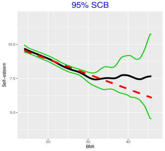
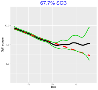
Figure 3: Plots of the weighted local linear estimate $\hat{m}(x,\hat{\pi})$ (thick solid line), the $95\%$ and $67.7\%$ SCBs (solid lines), and the null hypothesis weighted linear regression curve (dashed line) for the youth student survey data collected from white female students.

As an illustration, our proposed SCB is applied to the data collected from the Canada 2010/2011 Youth Student Survey to study the relationship between self-esteem and BMI. Figure 3 depicts the weighted local linear estimator and the SCB for the data. The null hypothesis of the mean function $m(x)=a+bx$ for some constants $a$ and $b$ is tested by our SCB with the minimum confidence level covering the null curve being $67.7\%$. Hence, with the $p$-value of $0.323$ one cannot reject the null hypothesis; see Section 6 for more details.

The rest of the paper is organized as follows. Section 2 presents the main theoretical results and the detailed procedure to implement the proposed method. Finite sample simulation results and real data analyses are reported in Sections 3 and 4, respectively. Proofs of the main results are provided in the Appendix and the online Supplementary Materials.

2. Main Results 2.1 A new SCB for the mean function

When samples $\left(X_{i},Y_{i}\right)$ are fully observable, Fan and Gijbels (1996) proposed the local linear regression method to estimate $m\left(x\right)$ by solving

$$\text{argmin}_{\beta_{0},\beta_{1}\in\mathbb{R}}n^{-1}\sum\limits_{i=1}^{n}\left\{Y_{i}-\beta_{0}-\beta_{1}\left(X_{i}-x\right)\right\}^{2}K_{h}\left(X_{i}-x\right),$$ (2)

where $K_{h}\left(\cdot\right)=h^{-1}K\left(\cdot/h\right)$ is a rescaled kernel function with bandwidth $h$. However, when covariates are MAR, the complete case analysis in (2) by using only fully observed ($X_{i}$, $Y_{i}$) can result in biased estimator for $m(x)$. Assume that the observed data are $(\delta_{i},\delta_{i}X_{i},Y_{i})$, $i=1,\dots,n$, where $\delta_{i}=1$ if $X_{i}$ is observed and $\delta_{i}=0$ otherwise, and $\pi_{i}=P\left(\delta_{i}=1|Y_{i},X_{i}\right)=P\left(\delta_{i}=1|Y_{i}\right)=\pi\left(Y_{i}\right)$ is the selection probability by our MAR assumption. To accommodate the missingness, we apply the Horvitz-Thompson inverse selection weighted method by minimizing the following quantity with respect to $(\beta_{0},\beta_{1}),$

$$n^{-1}\sum\limits_{i=1}^{n}\frac{\delta_{i}}{\pi_{i}}\left\{Y_{i}-\beta_{0}-\beta_{1}\left(X_{i}-x\right)\right\}^{2}K_{h}\left(X_{i}-x\right),$$ (3)

By least squares, one obtains the estimator $\hat{m}\left(x,\pi\right)$ for $m(x)$ with

$$\hat{m}\left(x,\pi\right)=e_{0}^{T}\left(\mathbf{X}^{T}\mathbf{WX}\right)^{-1}\mathbf{X}^{T}\mathbf{WY,}$$ (4)

where

$$\mathbf{X=}\left(\begin{array}[]{ccc}1&\cdots&1\\ X_{1}-x&\cdots&X_{n}-x\end{array}\right)^{T},$$

$\mathbf{W=}\frac{1}{n}\mathop{\mathrm{d}iag}\left(\frac{\delta_{1}}{\pi_{1}}K_{h}\left(X_{1}-x\right),\dots,\frac{\delta_{n}}{\pi_{n}}K_{h}\left(X_{n}-x\right)\right)$, $\mathbf{Y}=\left(Y_{1},\dots,Y_{n}\right)^{T}$, and $e_{0}=\left(1,0\right)^{T}$. Here $\hat{m}\left(x,\pi\right)$ is used to emphasize its dependence on the selection probability function $\pi(y)$.

Note that the selection probability function $\pi(y)$ is generally unknown. Here we assume that $\pi\left(y\right)$ follows a parametric binary model $\pi\left(y,\mathbf{\alpha}\right)$ where $\mathbf{\alpha}$ is some unknown parameter vector. For example, assuming a logistic regression model, $\pi_{i}=\pi\left(Y_{i},\mathbf{\alpha}\right)=P(\delta_{i}=1|Y_{i})=\{1+\exp\left(-\alpha_{0}-\alpha_{1}Y_{i}\right)\}^{-1}$, $\mathbf{\alpha=}\left(\alpha_{0},\alpha_{1}\right)^{T}$. By applying the maximum likelihood approach, one easily obtains a root-$n$ consistent estimate $\mathbf{\hat{\alpha}}$; see Robins et al. (1994) and Wang et al. (1998) for related studies and Hosmer and Lemeshow (2005) for a global statistic test for examining the pre-assumed binary regression model. Denote the resulting selection probability function estimator as $\hat{\pi}\left(y\right)=\hat{\pi}(y,\mathbf{\hat{\alpha}})$ and let $\hat{\pi}_{i}=\hat{\pi}\left(Y_{i},\mathbf{\hat{\alpha}}\right)$, $i=1,\dots,n$. Thus, replacing $\pi_{i}$ in (3) with $\hat{\pi}_{i}$, the feasible weighted estimator $\hat{m}\left(x,\hat{\pi}\right)$ of $m\left(x\right)$ is derived with

$$\hat{m}\left(x,\hat{\pi}\right)=e_{0}^{T}\left(\mathbf{X}^{T}\mathbf{\hat{W}X}\right)^{-1}\mathbf{X}^{T}\mathbf{\hat{W}Y,}$$ (5)

where the symbols with a hat on the right side of the equation above are the same as those in equation (4) but with $\pi_{i}$ replaced by $\hat{\pi}_{i}$.

For any function $\phi\left(x\right)$, we use $\phi^{\left(s\right)}(x)$ to represent its $s$-th order derivative, and for any integer $p\geq 0$ and use $C^{\left(p\right)}\left[c,d\right]$ to indicate the space of functions that have continuous $p$-th derivative on the interval $\left[c,d\right]$ with letting $C\left[c,d\right]=C^{\left(0\right)}\left[c,d\right]$. For any real positive sequences $l_{n}$ and $d_{n},$ $l_{n}\ll d_{n}$ means $l_{n}/d_{n}\rightarrow 0$ as $n\rightarrow\infty$.

To construct an accurate SCB for the mean function $m(x)$, we need the following general assumptions:

1. The mean function $m\left(x\right)\in C^{\left(2\right)}\left[a,b\right]$ and the density function $f_{X}\left(x\right)$ of $X$ is positive in the open interval $\left(a,b\right)$ with $f_{X}\left(x\right)\in C^{(1)}\left[a,b\right]$. Moreover, the joint density function $f_{X,\varepsilon}\left(x,\varepsilon\right)$ of $\left(X,\varepsilon\right)$  has continuous first order partial derivative with respect to $x$.

2. The variance function $\sigma^{2}(x)$ is bounded on $\left[a,b\right]$ and $\mathop{\textstyle\int}\varepsilon^{2}f_{X,\varepsilon|\delta=1}\left(x,\varepsilon\right)d\varepsilon$  has a positive lower bound for all $x\in\left[a,b\right]$, where $f_{X,\varepsilon|\delta=1}\left(x,\varepsilon\right)$ is the joint density function of $\left(X,\varepsilon\right)$ given $\delta=1$. In addition, there exist constants $\eta>4$ and $M_{\eta}>0$ such that $\mathop{\mathrm{E}}(\left|\varepsilon\right|^{2+\eta}\big{|}X)\leq M_{\eta}$ a.s.

3. The kernel function $K\left(\cdot\right)$ is a symmetric probability density function supported on $\left[-1,1\right]$ and $\in C^{\left(1\right)}\left[\mathbb{-}1,1\right]$.

4. The selection probability function $\pi\left(y\right)$ follows a parametric binary model and has a positive lower bound $c_{\pi}$. Moreover, it has bounded second order partial derivative with respect to $y$ and has bounded first order partial derivative with respect to $\mathbf{\alpha.}$

5. The bandwidth $h=h_{n}$ satisfies $n^{-1/3}\log n\ll h\ll n^{-1/5}\log^{-1/5}n$.

Assumptions (A1)–(A3) are elementary conditions in nonparametric kernel regression adapted from Johnston (1982), Härdle (1989), Wang and Yang (2009), and Cai et al. (2019b). Assumption (A1) implies that for any compact subinterval $\left[a_{0},b_{0}\right]\subset\left(a,b\right)$, there exist positive constants $c_{f},C_{f}$ such that $c_{f}\leq f_{X}\left(x\right)\leq C_{f}$, $\forall x\in\left[a_{0},b_{0}\right]$. The condition $\eta>4$ in Assumption (A2) can be relaxed to $\eta>3$ but then the lower order restriction of the bandwidth is more complicated. For simplicity here we use $\eta>4$. Assumption (A3) entails that $\mu_{0}\left(K\right)=1$ and $\mu_{1}\left(K\right)=0$ where $\mu_{l}\left(K\right)=\mathop{\textstyle\int}\nolimits_{-1}^{1}u^{l}K\left(u\right)du,l=0,1$. Assumption (A4) is typical in the missing data analysis. The same condition appears in Liang et al. (2004) and Wang et al. (1997). Assumption (A5) is about the choice of bandwidth $h$. Technically, it keeps the bias at a lower rate than the variance and entails some negligible nonlinear remainder terms.

For any functions $\varphi_{n}\left(x\right)$ and $\phi_{n}\left(x\right),x\in\mathcal{D}$, we use $\varphi_{n}\left(x\right)=$ $O\left(\phi_{n}\left(x\right)\right)$ and $\varphi_{n}\left(x\right)=o\left(\phi_{n}\left(x\right)\right)$ to mean “$\varphi_{n}\left(x\right)/\phi_{n}\left(x\right)$ is bounded and $\varphi_{n}\left(x\right)/\phi_{n}\left(x\right)$ tends to $0$ as $n\rightarrow\infty$ for any fixed $x\in\mathcal{D}$”, while use $\varphi_{n}\left(x\right)=$ $U\left(\phi_{n}\left(x\right)\right)$ and $\varphi_{n}\left(x\right)=u\left(\phi_{n}\left(x\right)\right)$ to mean “$\varphi_{n}\left(x\right)/\phi_{n}\left(x\right)$ is bounded and $\varphi_{n}\left(x\right)/\phi_{n}\left(x\right)$ tends to $0$ as $n\rightarrow\infty$ for all $x\in\mathcal{D}$ uniformly”. We use $O_{p}$, $o_{p}$, $U_{p}$ and $u_{p}$ to represent the corresponding terms in probability.

Theorem 1.

Under Assumptions (A1)–(A5), as $n\rightarrow\infty$, for any $x\in\left[a_{0},b_{0}\right]$, one has

$$\hat{m}\left(x,\pi\right)-m\left(x\right)=R_{n}\left(x\right)+2^{-1}h^{2}\mu_{2}\left(K\right)m^{\left(2\right)}\left(x\right)\!+u_{p}\left(h^{2}\right),$$

where $R_{n}\left(x\right)=n^{-1}f_{X}^{-1}\left(x\right)\sum\limits_{i=1}^{n}\frac{\delta_{i}}{\pi_{i}}K_{h}\left(X_{i}\!-\!x\right)\varepsilon_{i}$.

The proof of Theorem 1 is given in the Appendix. Together with $h\ll n^{-1/5}\log^{-1/5}\!n$, one can easily obtain that

$$\sup_{x\in\left[a_{0},b_{0}\right]}\left|\hat{m}\left(x,\pi\right)-m\left(x\right)\right|=\sup_{x\in\left[a_{0},b_{0}\right]}\left|R_{n}\left(x\right)\right|+O_{p}\left(h^{2}\right).$$ (6)

Lemma S.2 in the Supplementary Materials shows that $\sup_{x\in[a_{0},b_{0}]}\!\left|R_{n}(x)\right|\!=\!O_{p}(n^{-1/2}h^{-1/2}\!\log^{1/2}\!n)$ which implies that the dominating term of $\sup_{x\in[a_{0},b_{0}]}$ $\left|\hat{m}\left(x,\pi\right)-m\left(x\right)\right|$ is $\sup_{x\in[a_{0},b_{0}]}\left|R_{n}(x)\right|$.

Let $\Delta_{n}=\sum_{i=1}^{n}\delta_{i}$ be the number of complete cases and denote the ratio by $r_{n}=\Delta_{n}/n$. Since $\delta_{1},\dots,\delta_{n}$ are i.i.d., it is readily seen that

$$r_{n}=P\left(\delta_{1}=1\right)+O_{p}(n^{-1/2}).$$ (7)

We now give the following theorem which describes the limiting distribution of the maximal deviation between $\hat{m}\left(x,\pi\right)$ and $m\left(x\right)$. Its proof is given in the Appendix.

Theorem 2.

Under Assumptions (A1)–(A5), as $n\rightarrow\infty$, for any $t\in\mathbb{R},$

$$P\left\{a_{h}\left[\sup_{x\in\left[a_{0},b_{0}\right]}\left|\frac{\left(nh\right)^{1/2}r_{n}^{-1/2}\left\{\hat{m}\left(x,\pi\right)-m\left(x\right)\right\}}{d^{1/2}\left(x\right)}\right|-b_{h}\right]\leq t\right\}$$

$$\rightarrow\exp\left\{-2\exp\left(-t\right)\right\},$$ (8)

where

$$a_{h}=\sqrt{-2\log\left(h/\left(b_{0}-a_{0}\right)\right)},b_{h}=a_{h}+2^{-1}a_{h}^{-1}\log\left(4^{-1}\pi^{-2}C\left(K\right)\right),$$

$$d\left(x\right)=\lambda\left(K\right)s\left(x\right)f_{X}^{-2}\left(x\right),s\left(x\right)=\int\frac{\varepsilon^{2}}{\pi^{2}\left(m\left(x\right)+\varepsilon\right)}f_{X,\varepsilon|\delta=1}\left(x,\varepsilon\right)d\varepsilon,$$

$$\lambda\left(K\right)=\mathop{\textstyle\int}\nolimits_{-1}^{1}K^{2}\left(u\right)du,C\left(K\right)=\lambda^{-1}\left(K\right)\mathop{\textstyle\int}\nolimits_{-1}^{1}\left\{K^{\left(1\right)}\left(u\right)\right\}^{2}du.$$

Note that when data are fully observed, i.e., $\pi\left(y\right)\equiv 1,r_{n}\equiv 1$, $s\left(x\right)$ becomes $\sigma^{2}\left(x\right)f_{X}\left(x\right)$. In such a case, the result degenerates to that for the local linear estimator for fully observed data, which extends the result of Johnston (1982) for the Nadaraya-Watson kernel estimator to the local linear estimator under more general conditions.

The proof of Theorem 2 is quite involved. It uses the total probability formula that the probability of the dominating term $\sup_{x\in\left[a_{0},b_{0}\right]}\!\left|\left(nh\right)^{1/2}r_{n}^{-1/2}\right.$ $\left.R_{n}(x)/d^{1/2}\left(x\right)\right|$ is the weighted average of its conditional probability given $\Delta_{n}=n_{0}$ with weights $P(\Delta_{n}=n_{0}),n_{0}=0,1,2,...,n$; see the detailed argument in the Appendix. In the rest theoretical development, we assume that the parametric model for $\pi$ is correctly specified so that the estimator $\mathbf{\hat{\alpha}}$ satisfies $\mathbf{\hat{\alpha}}-\mathbf{\alpha}=O_{p}(n^{-1/2})$. Theorem 3 below compares the difference between the estimator based on the true selection probability function $\pi$ and that based on the estimated selection probability function $\hat{\pi}$. Its proof is given in the Appendix.

Theorem 3.

Under Assumptions (A1)–(A5), as $n\rightarrow\infty$,

$$\sup_{x\in\left[a_{0},b_{0}\right]}\left|\hat{m}\left(x,\hat{\pi}\right)-\hat{m}\left(x,\pi\right)\right|=O_{p}\left(n^{-1/2}\right).$$

Combining Theorems 2 and 3 and Slutsky’s Theorem, one obtains the following result:

Theorem 4.

Under Assumptions (A1)–(A5), as $n\rightarrow\infty$, for any $t\in\mathbb{R},$

$$P\left\{a_{h}\left[\sup_{x\in\left[a_{0},b_{0}\right]}\left|\frac{\left(nh\right)^{1/2}r_{n}^{-1/2}\left\{\hat{m}\left(x,\hat{\pi}\right)-m\left(x\right)\right\}}{d^{1/2}\left(x\right)}\right|-b_{h}\right]\leq t\right\}$$

$$\rightarrow\exp\left\{-2\exp\left(-t\right)\right\}.$$

Theorem 4 above can be used to construct a theoretical SCB for $m\left(x\right)$ which depends on unknown quantity $d\left(x\right)$. To obtain a feasible SCB, we estimate $d\left(x\right)$ by

$$\hat{d}_{n}\left(x\right)=\Delta_{n}^{-1}h\hat{f}_{X}^{-2}\left(x\right)\mathop{\displaystyle\sum}\limits_{i=1}^{n}\frac{\delta_{i}}{\hat{\pi}_{i}^{2}}K_{h}^{2}\left(X_{i}\!-\!x\right)\hat{\varepsilon}_{i}^{2},$$

where $\hat{\varepsilon}_{i}=Y_{i}-\hat{m}\left(X_{i},\hat{\pi}_{i}\right)$ and $\hat{f}_{X}\left(x\right)$ is the weighted kernel density pilot estimator of $f_{X}\left(x\right)$ with

$$\hat{f}_{X}\left(x\right)=n^{-1}\sum\limits_{i=1}^{n}\frac{\delta_{i}}{\hat{\pi}_{i}}K_{h_{f}}\left(X_{i}\!-\!x\right),$$ (9)

in which we recommend to use the Silverman’s rule-of-thumb bandwidth (Silverman (1986), p.48) computed with complete data for $h_{f}$ which has the order of $n^{-1/5}$.

Theorem 5.

Under Assumptions (A1)–(A5), as $n\rightarrow\infty$, one has

$$\sup_{x\in\left[a_{0},b_{0}\right]}\left|\hat{d}_{n}\left(x\right)-d\left(x\right)\right|=O_{p}\left(n^{-1/2}h^{-3/2}\log^{1/2}n\right)\text{.}$$

Note that $n^{-1/2}h^{-3/2}\log^{1/2}n\ll\log^{-1}n$ by Assumption (A5). Therefore, we have the following corollary.

Corollary 1.

Under Assumptions (A1)–(A5), for any $\alpha\in\left(0,1\right)$, an asymptotic $100\left(1-\alpha\right)\%$ simultaneous confidence band for $m\left(x\right)$ over $\left[a_{0},b_{0}\right]$ is

$$\hat{m}\left(x,\hat{\pi}\right)\pm\left(nh\right)^{-1/2}r_{n}^{1/2}\hat{d}_{n}^{1/2}\left(x\right)\left(b_{h}+a_{h}^{-1}q_{\alpha}\right),$$ (10)

where $q_{\alpha}=-\log\left\{-\frac{1}{2}\log\left(1-\alpha\right)\right\}$ and $a_{h}$, $b_{h}$ are given in Theorem 2.

2.2 Implementation

In this subsection, we describe the detailed procedure to implement the asymptotic SCB in (10). They will be used throughout Section 3 and Section 4 for simulation studies and real data analysis.

The range of the covariate variable is taken as ${\small[\hat{a},\hat{b}]}$ with $\hat{a}=\min_{\{1\leq i\leq n,\,\delta_{i}=1\}}$ $X_{i}$ and $\hat{b}=\max_{\{1\leq i\leq n,\,\delta_{i}=1\}}X_{i}$, while the compact subinterval ${\small[\hat{a}_{0},\hat{b}_{0}]}$ with $\hat{a}_{0}=0.9\hat{a}+0.1\hat{b}$ and $\hat{b}_{0}=0.9\hat{b}+0.1\hat{a}$ is regarded as the interval over which the SCBs are constructed. The quartic kernel, $K\left(u\right)=15\left(1-u^{2}\right)^{2}I\left(\left|u\right|\leq 1\right)$ $/16$, is used for the weighted local linear estimator in (5) and the weighted kernel density estimator in (9), satisfying Assumption (A3).

Regarding the bandwidth selection for $\hat{m}$ in (4), we adopt $h=h_{\text{rot}}\log^{-\rho}n$ for some $\rho>1/5$, where $h_{\text{rot}}$ is the rule-of-thumb bandwidth in Fan and Gijbels (1996, Equation (4.3)) computed with the complete data. Note that the order of $h_{\text{rot}}$ is $n^{-1/5}$ and hence the order of $h$ is $n^{-1/5}\log^{-\rho}n$ which satisfies Assumption (A5). We have found in extensive simulations that $h=h_{\text{rot}}\log^{-1/4}n$ (i.e., $\rho=1/4$) works quite well and that is what we recommend.

3. Simulation Studies

In this section, we investigate the finite sample behaviors of the proposed SCB and the finite sample effect due to estimating the selection probabilities. For comparison, we also list the results of the complete case SCB for local linear regression by directly ignoring the missing covariates, denoted by SCB-CC.

The following four cases were examined:

Case 1 : $$m\left(X\right)=\sin\left(\pi X\right),\sigma\left(X\right)=1;$$

Case 2 : $$m\left(X\right)=\sin\left(\pi X\right),\sigma\left(X\right)=2\exp(X)\left\{\exp(X)+1\right\}^{-1};$$

Case 3 : $$m\left(X\right)=\exp(-6X^{3}/5),\sigma\left(X\right)=1;$$

Case 4 : $$m\left(X\right)=\exp(-6X^{3}/5),\sigma\left(X\right)=2\exp(X)\left\{\exp(X)+1\right\}^{-1},$$

where $X\sim U\left[-1,1\right]$, and the error $\varepsilon\sim N\left(0,\sigma^{2}\left(x\right)\right)$. Clearly, these scenarios include both homoscedastic errors (Case 1, Case 3) and heteroscedastic errors (Case 2, Case 4). Two models for the selection probability function were considered: (i) logistic model $\pi\left(Y\right)=P\left(\delta=1|Y\right)=\left\{1+\exp(-\alpha_{0}-\alpha_{1}Y)\right\}^{-1}$, and (ii) probit model $\pi\left(Y\right)=P\left(\delta=1|Y\right)=\Phi\left(\alpha_{0}^{\ast}+\alpha_{1}^{\ast}Y\right)$, where $\Phi$ is the standard normal cumulative distribution function. We took $\left(\alpha_{0},\alpha_{1}\right)$ and $\left(\alpha_{0}^{\ast},\alpha_{1}^{\ast}\right)$ as $(1.8,1)$ and $(1,0.5)$, respectively, leading to approximately $8\%$ to $20\%$ of the data missing (low proportion of missing). We also took $\left(\alpha_{0},\alpha_{1}\right)$ and $\left(\alpha_{0}^{\ast},\alpha_{1}^{\ast}\right)$ as $(0.2,0.6)$ and $(0.1,0.3)$, respectively, leading to approximately $31\%$ to $46\%$ of the data missing (high proportion of missing). The sample sizes were $n=400,600,800$ and the confidence levels were $1-\alpha=0.95,0.99$.

We first look at the performance of the proposed SCB in the cases where the selection probability models are correctly specified. Tables 1–4 give the coverage frequencies over 1000 replications that the true mean function was covered by the SCB in (10) and the SCB-CC at the equally spaced points $\hat{a}_{0}+(\hat{b}_{0}-\hat{a}_{0})k/400$, $k=0,\dots,400$. One can see that for all scenarios, the coverage frequencies of the proposed SCB in (10) are close to the nominal confidence levels $0.95$ and $0.99$ while the coverage frequencies of SCB-CC are far lower than the nominal levels, and the average lengths of SCB-CC are systematically narrower than that of the proposed SCB. Meanwhile, the average lengths of the SCBs decrease as the sample size $n$ increases, as expected. All in all, it can be seen that the proposed SCB in (10) performs much better than the SCB-CC. This is because the local linear estimation in the complete case is generally biased for the underlying true function. These findings confirm our theoretical results.

We next investigate the sensitivity of the SCB to the selection probability model misspecification. Similar to Wang et al. (1997), we carried out a simulation study which is similar to that in Table 2 except that the selection probability is truncated above by $0.75$. As a result, about $46\%$ of the cases had missing covariates. Therefore, using the logistic regression model to fit $\pi(y)$ is not completely correct in this setting. Table 5 summarizes the simulation results under this misspecification. One can see that for all the scenarios, the coverage frequencies are quite close to those under the correct specification of $\pi(y)$. It suggests that the proposed SCB is not very sensitive to misspecification of the selection probability function.

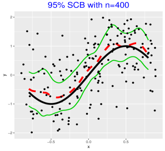
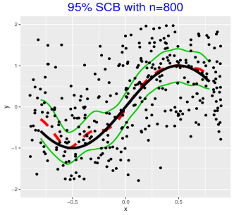
Figure 1: Plots of the true mean function $m(x)$(thick solid line), the weighted local linear estimate $\hat{m}(x,\hat{\pi})$ (dashed line) and the $95\%$ SCB (solid line) for Case 1 under the selection probability model (i) with parameters $(\alpha_{0},\alpha_{1})=(0.2,0.6)$ (about $45\%$ missing).

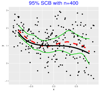
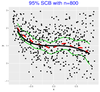
Figure 2: Plots of the true mean function $m(x)$ (thick solid line), the weighted local linear estimate $\hat{m}(x,\hat{\pi})$ (dashed line) and the $95\%$ SCB (solid line) for Case 4 under the selection probability model (i) with parameters $(\alpha_{0},\alpha_{1})=(0.2,0.6)$ (about $31\%$ missing).

To visualize the SCB for the mean function, Figures 1 and 2 were created based on two samples of size 400 and 800 for Case 1 and Case 4 under the logit missing mechanism with $\left(\alpha_{0},\alpha_{1}\right)=(0.2,0.6)$. One can see that the SCB for $n=800$ is narrower and fits the true mean function better than those for $n=400$, which corroborates our asymptotically theoretical results. We have also created the figures in other cases, and the results are similar.

4. Real Data Analysis

In this section, we illustrate an application to the data from the Canada 2010/2011 Youth Student Survey. The 2010/2011 Youth Student Survey sponsored by Health Canada is a pan-Canadian, classroom-based survey on a representative youth students in grades $6$–$12$ between October 2010 and June 2011. It aims to provide Health Canada, provinces, schools, communities, and parents with timely and reliable data on tobacco, alcohol and drug use in addition to other related issues about Canadian students; see more details in 2010-2011 YSS Student Survey Data Codebook or from https://uwaterloo.ca/canadian-student-tobacco-alcohol-drugs-survey.

We focused on a subset of the data collected from white female youth students in grades $6$–$12$ to study the relationship between self-esteem and Body Mass Index (BMI); see the interesting related discussions and further references in Habib et al. (2015) and Al Ahmari et al. (2017). In this data set, the self-esteem was measured by using a score ranging from $0$ to $12$, and the BMI was computed by the weight over height in meter squared, ranging from $10.04$ to $49.78$. There were a total of $5343$ students with having complete observations on self-esteem, while only $3565$ students provided BMI ($33.2\%$ missing rate).

For the data missingness mechanism, we used the logistic regression to estimate $\pi(y)$. The fitted estimates are $\hat{\mathbf{\alpha}}=(0.82585,-0.015)^{T}$. To further judge how well the model fits the missingness pattern in the data, the Hosmer-Lemeshow goodness of fit test was employed with the $p$-value $=0.17$. Thus one cannot reject the null hypothesis that the logistic model is correct. Figure 3 shows the inverse selection probability weighted local linear estimate $\hat{m}(x,\hat{\pi})$ (thick solid line) and the $95\%$ and $65.6\%$ SCBs (solid lines). The SCB was applied to test the null hypothesis $H_{0}:m(x)=a+bx$ where the coefficients $(a,b)^{T}$ were computed by the inverse selection probability weighted least square method; see the null curve (dashed line) in Figure 3. One can see that the null curve is completely covered by the $95\%$ SCB. Thus the null hypothesis of the mean function being a linear function cannot be rejected at the significant level $=0.05$. Applying Theorem 4, we obtained that the minimum confidence level containing the null curve is $67.7\%$; see the right panel of Figure 3. Therefore, the null hypothesis cannot be rejected with $p$-value $=0.323$.

Moreover, one can also see that the mean curve has a general decreasing trend, i.e., there is a negative association between self-esteem and BMI among white female youth students in grades $6$–$12$. This result agrees with that discovered by Habib et al. (2015). Meanwhile, according to Habib et al. (2015), a BMI between $20$ and $25$ is considered normal, a BMI between $25$ and $30$ is considered overweight, and a BMI $>30$ is considered obese. Therefore, even if female students were within normal weight range, their self-esteem was still decreased as BMI increased. This may be because female students in general are more likely to see themselves as obese or overweight and show dissatisfaction with their body image even if they have a healthy weight.

5. Concluding Remarks

In this paper, an asymptotically accurate SCBs were constructed for the nonparametric mean function with covariates missing at random by employing the weighted estimator based on inverse selection probabilities. The limiting distribution of the global estimation error (also known as maximal deviation) was derived, overcoming the main technical challenge on formulating such a confidence band. The proposed estimator for the mean function was shown to be oracally efficient in the sense that using root-$n$ consistent selection probability estimates is as efficient as that when the selection probabilities were known as a prior. Simulation studies confirm our theoretical findings and the analysis of the Canada 2010/2011 Youth Student Survey data illustrates the versatility of the SCB. The methodology should also be suitable to partial linear models for missing covariates data (Wang (2009)). Further investigations may lead to similar constructions of SCBs for generalized nonparametric models, partial linear single-index models and functional data with covariates missing at random.

5. Supplementary Materials

The online Supplementary Materials contain some lemmas to be used in the proofs of the main theorems in Section 2.

Acknowledgements

This research was supported in part by the National Natural Science Foundation of China Award NSFC #11701403, #11901521, First Class Discipline of Zhejiang–A (Zhejiang Gongshang University–Statistics), a grant from the Key Lab of Random Complex Structure and Data Science, CAS, China, and the Simons Foundation Mathematics and Physical Sciences Program Award #499650.

Appendix

We use $a_{n}\sim b_{n}$ to represent $\lim_{n\rightarrow\infty}a_{n}/b_{n}=c,$ where $c$ is some nonzero constant. For any function $\varphi\left(u\right)$ defined on $\left[a,b\right]$, let $\left\|\varphi\left(u\right)\right\|_{\infty}=\left\|\varphi\right\|_{\infty}=\sup_{u\in\left[a,b\right]}\left|\varphi\left(u\right)\right|$.

A.1 Conditional limiting extreme value distribution of $R_{n}(x)$

This section contains the main steps to obtain the conditional extreme value distribution of $R_{n}(x)=n^{-1}f_{X}^{-1}\left(x\right)\sum\limits_{i=1}^{n}\frac{\delta_{i}}{\pi_{i}}K_{h}\left(X_{i}\!-\!x\right)\varepsilon_{i}$ shown in Theorem A.1 at the end of this section which will be used in the total probability formula in the proof of Theorem 2.

The Rosenblatt quantile transformation in Rosenblatt (1952) is adopted with

$$T\left(X,\varepsilon\right)=\left(X^{\ast},\varepsilon^{\ast}\right)=\left(F_{X|\delta=1}\left(X\right),F_{\varepsilon|X,\delta=1}\left(\varepsilon|X\right)\right),$$

where $F_{X|\delta=1}\left(X\right)$ is the conditional distribution function of $X$ given $\delta=1$ and $F_{\varepsilon|X,\delta=1}\left(\varepsilon|X\right)$ is the conditional distribution function of $\varepsilon$ given $X$ and $\delta=1$. This transformation produces mutually independent uniform random variables $\left(X^{\ast},\varepsilon^{\ast}\right)$ on $\left[0,1\right]^{2}$. According to the strong approximation theorem in Tusnády (1977) (Theorem 1), there exists a sequence of two dimensional Brownian bridges $B_{n}$ such that

$$\sup\nolimits_{x,\varepsilon}\left|Z_{n}\left(x,\varepsilon\right)-B_{n}\left(T\left(x,\varepsilon\right)\right)\right|=O\left(n^{-1/2}\log^{2}n\right)\text{ a.s.},$$ (A.1)

where $Z_{n}\left(x,\varepsilon\right)=n^{1/2}\left\{F_{n}\left(x,\varepsilon\right)-F_{X,\varepsilon|\delta=1}\left(x,\varepsilon\right)\right\}$ with $F_{n}\left(x,\varepsilon\right)$ and $F_{X,\varepsilon|\delta=1}$ $\left(x,\varepsilon\right)$ representing the empirical and the theoretical distribution of $\left(X,\varepsilon\right)$ given $\delta=1$. The transformation and the strong approximation results have been also used in Johnston (1982), Härdle (1989), and Wang and Yang (2009) for constructing SCBs for the nonparametric regression when data is fully observed.

To obtain the distribution of $\sup_{x\in\left[a_{0},b_{0}\right]}\left|R_{n}(x)\right|$ conditional on $\Delta_{n}=n_{0}$, we will show the following Lemmas A.1–A.3. Here $\{n_{0}\}$ is a sequence of numbers related to $n$ with $1\leq n_{0}\leq n$. By (7) it is clear that $n\to\infty$ if and only if $n_{0}\to\infty$ in probability. Meanwhile, due to the i.i.d. assumption of the data, conditional on $\Delta_{n}=n_{0}$ is equivalent to conditional on $\mathbf{\delta}_{n}=\left(\delta_{1},...,\delta_{n}\right)^{T}$ in which $n_{0}$ of the $\delta_{i}$ equal to 1 and the rest $\delta_{i}$ equal to 0. Without loss of generality, let $\delta_{i}=1$ for $i=1,\dots,n_{0}$ and $\delta_{i}=0$ for $i=n_{0}+1,\dots,n$.

Notice that, for $i=1,\dots,n$,

$$0 = \mathop{\mathrm{E}}\!\left\{\frac{\delta_{i}}{\pi_{i}}K_{h}\left(X_{i}\!-\!x\right)\varepsilon_{i}\right\}=\mathop{\mathrm{E}}\left[\mathop{\mathrm{E}}\!\left\{\left.\frac{\delta_{i}}{\pi_{i}}K_{h}\left(X_{i}\!-\!x\right)\varepsilon_{i}\right|\delta_{i}\right\}\right]$$

$$= \mathop{\mathrm{E}}\left\{\left.\frac{1}{\pi_{i}}K_{h}\left(X_{i}\!-\!x\right)\varepsilon_{i}\right|\delta_{i}=1\right\}P\left(\delta_{i}=1\right).$$

Thus, conditional on $\Delta_{n}=n_{0}$, $1\leq n_{0}\leq n$, by symmetry one has

$$\mathop{\mathrm{E}}\left\{\left.\mathop{\displaystyle\sum}\limits_{i=1}^{n}\frac{\delta_{i}}{\pi_{i}}K_{h}\left(X_{i}\!-\!x\right)\varepsilon_{i}\right|\Delta_{n}=n_{0}\right\}\!\!\!\!$$

$$=\mathop{\mathrm{E}}\left\{\left.\mathop{\displaystyle\sum}\limits_{i=1}^{n}\frac{\delta_{i}}{\pi_{i}}K_{h}\left(X_{i}\!-\!x\right)\varepsilon_{i}\right|\delta_{1}=\cdots=\delta_{n_{0}}=1,\delta_{n_{0}+1}=\cdots=\delta_{n}=0\right\}$$

$$=n_{0}\mathop{\mathrm{E}}\left\{\left.\frac{1}{\pi_{1}}K_{h}\left(X_{1}\!-\!x\right)\varepsilon_{1}\right|\delta_{1}=1\right\}=0\text{ a.s.}$$

and

$$\mathop{\mathrm{v}ar}\!\left\{\left.\mathop{\textstyle\sum}\limits_{i=1}^{n}\frac{\delta_{i}}{\pi_{i}}K_{h}\left(X_{i}\!-\!x\right)\varepsilon_{i}\right|\Delta_{n}=n_{0}\right\}$$

$$=\mathop{\mathrm{E}}\left\{\left.\{\mathop{\displaystyle\sum}\limits_{i=1}^{n}\frac{\delta_{i}}{\pi_{i}}K_{h}\left(X_{i}\!-\!x\right)\varepsilon_{i}\}^{2}\right|\delta_{1}=\cdots=\delta_{n_{0}}=1,\delta_{n_{0}+1}=\cdots=\delta_{n}=0\right\}$$

$$=n_{0}\mathop{\mathrm{E}}\!\left(\left.\frac{1}{\pi_{1}^{2}}K_{h}^{2}\left(X_{1}\!-\!x\right)\varepsilon_{1}^{2}\right|\delta_{1}=1\right)$$

$$=n_{0}\int\frac{1}{\pi^{2}\left(m\left(u\right)+\varepsilon\right)}K_{h}^{2}\left(u\!-\!x\right)\varepsilon^{2}f_{X,\varepsilon|\delta=1}\left(u,\varepsilon\right)dud\varepsilon$$

$$=n_{0}h^{-1}\int\frac{1}{\pi^{2}\left(m\left(x+hv\right)+\varepsilon\right)}K^{2}\left(v\right)\varepsilon^{2}f_{X,\varepsilon|\delta=1}\left(x+hv,\varepsilon\right)dvd\varepsilon$$

$$=n_{0}h^{-1}\int K^{2}\left(v\right)dv\int\frac{1}{\pi^{2}\left(m\left(x\right)+\varepsilon\right)}\varepsilon^{2}f_{X,\varepsilon|\delta=1}\left(x,\varepsilon\right)d\varepsilon\left\{1+u_{p}\left(1\right)\right\}$$

$$=n_{0}h^{-1}\lambda\left(K\right)s\left(x\right)\left\{1+u_{p}\left(1\right)\right\},$$ (A.2)

where $\lambda\left(K\right)$ and $s\left(x\right)$ are given in Theorem 2. Note that conditional on $\Delta_{n}=n_{0}$, without loss of generality, one can write

$$R_{n}\left(x\right)=n^{-1}f_{X}^{-1}\left(x\right)\sum\limits_{i=1}^{n_{0}}\frac{1}{\pi_{i}}K_{h}\left(X_{i}\!-\!x\right)\varepsilon_{i}.$$

Conditional on $\Delta_{n}=n_{0}$ we now introduce the following standardized stochastic process:

$$\zeta_{1n_{0}}\left(x\right)=\left(n_{0}h\right)^{1/2}s^{-1/2}\left(x\right)n_{0}^{-1}\mathop{\textstyle\sum}\limits_{i=1}^{n_{0}}\frac{1}{\pi_{i}}K_{h}\left(X_{i}\!-\!x\right)\varepsilon_{i},$$ (A.3)

which can be rewritten as

$$\zeta_{1n_{0}}\left(x\right)=h^{1/2}s^{-1/2}\left(x\right)\int\int\frac{1}{\pi\left(m\left(u\right)+\varepsilon\right)}K_{h}\left(u-\!x\right)\varepsilon dZ_{n_{0}}\left(u,\varepsilon\right),$$

where $Z_{n_{0}}\left(u,\varepsilon\right)$ is the same as $Z_{n}\left(u,\varepsilon\right)$ in (A.1) but with $n$ replaced by $n_{0}$.

Let $\kappa_{n}=n^{\theta}$ with $\frac{2}{3\eta}<\theta<\frac{1}{6}$ where $\eta>4$ is given in Assumption (A2), which together with Assumption (A5) implies that

$$\kappa_{n}^{-\eta}h^{-2}\left(\log n\right)=O\left(1\right),\text{ \ \ \ }\kappa_{n}^{2}n^{-1/2}h^{-1/2}\left(\log n\right)^{5/2}=o\left(1\right).$$ (A.4)

Then conditional on $\Delta_{n}=n_{0}$ one can define the following processes to approximate $\zeta_{1n_{0}}\left(x\right)$:

$$\zeta_{2n_{0}}\left(x\right) = h^{1/2}s_{n}^{-1/2}\left(x\right)\int\int_{\left|\varepsilon\right|\leq\kappa_{n}}\frac{1}{\pi\left(m\left(u\right)+\varepsilon\right)}K_{h}\left(u-\!x\right)\varepsilon dZ_{n_{0}}\left(u,\varepsilon\right),$$

$$\zeta_{3n_{0}}\left(x\right) = h^{1/2}s_{n}^{-1/2}\left(x\right)\int\int_{\left|\varepsilon\right|\leq\kappa_{n}}\frac{1}{\pi\left(m\left(u\right)+\varepsilon\right)}K_{h}\left(u-\!x\right)\varepsilon dB_{n_{0}}\left(T\left(u,\varepsilon\right)\right),$$

$$\zeta_{4n_{0}}\left(x\right) = h^{1/2}s_{n}^{-1/2}\left(x\right)\int\int_{\left|\varepsilon\right|\leq\kappa_{n}}\frac{1}{\pi\left(m\left(u\right)+\varepsilon\right)}K_{h}\left(u-\!x\right)\varepsilon dW_{n_{0}}\left(T\left(u,\varepsilon\right)\right),$$

where $s_{n}\left(x\right)=\int_{\left|\varepsilon\right|\leq\kappa_{n}}\varepsilon^{2}f_{X,\varepsilon|\delta=1}\left(x,\varepsilon\right)d\varepsilon,$ $B_{n_{0}}\left(T\left(u,\varepsilon\right)\right)$ is the sequence of Brownian bridges in (A.1) and $W_{n_{0}}\left(T\left(u,\varepsilon\right)\right)$ is the sequence of Wiener process satisfying $B_{n_{0}}\!\left(u,s\right)\!=\!W_{n_{0}}\!\left(u,s\right)$ $-usW_{n_{0}}\left(1,1\right)$. Moreover, define

$$\zeta_{5n_{0}}\left(x\right)=h^{1/2}s_{n}^{-1/2}\left(x\right)\int s_{n}^{1/2}\left(u\right)K_{h}\left(u-\!x\right)dW\left(u\right),$$

and

$$\zeta_{6n_{0}}\left(x\right)=h^{1/2}\int K_{h}\left(u-\!x\right)dW\left(u\right),$$

where $W\left(u\right)$ is a two-sided Wiener process on $\left(-\infty,+\infty\right)$. Conditional on $\Delta_{n}=n_{0}$, according to Theorem 3.1 in Bickel and Rosenblatt (1973), one has

$$P\left[\left.a_{h}\left\{\sup_{x\in\left[a_{0},b_{0}\right]}\left|\zeta_{6n_{0}}\left(x\right)\right|/\lambda^{1/2}\left(K\right)-b_{h}\right\}\leq t\right|\Delta_{n}=n_{0}\right]\rightarrow\exp\left\{-2\exp\left(-t\right)\right\}$$ (A.5)

$\forall t\in\mathbb{R}$, as $n_{0}$ (and thus $n$) $\to\infty$. Here $a_{h},b_{h}$, and $\lambda\left(K\right)$ are given in Theorem 2.

Lemma A.1.

Under Assumptions (A1)–(A5), conditional on $\Delta_{n}=n_{0}$, for an increasing sequence $\{n_{0}\}$, one has

$$(a)\sup_{x\in\left[a_{0},b_{0}\right]}\left|\zeta_{2n_{0}}\left(x\right)-\zeta_{3n_{0}}\left(x\right)\right|=o_{p}\left(\log^{-1/2}n\right),$$

$$(b)\sup_{x\in\left[a_{0},b_{0}\right]}\left|\zeta_{3n_{0}}\left(x\right)-\zeta_{4n_{0}}\left(x\right)\right|=o_{p}\left(\log^{-1/2}n\right),$$

$$(c)\sup_{x\in\left[a_{0},b_{0}\right]}\left|\zeta_{5n_{0}}\left(x\right)-\zeta_{6n_{0}}\left(x\right)\right|=o_{p}\left(\log^{-1/2}n\right),$$

as $n_{0}\to\infty$.

Proof of Lemma A.1(a). By integration by parts, one has

$$\zeta_{2n_{0}}\left(x\right)-\zeta_{3n_{0}}\left(x\right)$$

$$=h^{1/2}\left\{s_{n}\left(x\right)\right\}^{-1/2}\!\!\!\int\int_{\left|\varepsilon\right|\leq\kappa_{n}}\!\!\!\frac{K_{h}\left(u-\!x\right)\varepsilon}{\pi\left(m\left(u\right)+\varepsilon\right)}d\left\{Z_{n_{0}}\left(u,\varepsilon\right)\!\!-\!\!B_{n_{0}}\!\!\left(T\left(u,\varepsilon\right)\right)\right\}$$

$$=h^{-1/2}\left\{s_{n}\left(x\right)\right\}^{-1/2}\int_{-1}^{1}\int_{\left|\varepsilon\right|\leq\kappa_{n}}\frac{K\left(v\right)\varepsilon}{\pi\left(m\left(x+hv\right)+\varepsilon\right)}d\left\{Z_{n_{0}}\left(x+hv,\varepsilon\right)\!-\!B_{n_{0}}\!\left(T\left(x+hv,\varepsilon\right)\right)\right\}$$

$$=h^{-1/2}\left\{s_{n}\left(x\right)\right\}^{-1/2}\!\!\int_{-1}^{1}\int_{\left|\varepsilon\right|\leq\kappa_{n}}\!\!\left\{Z_{n_{0}}\left(x+hv,\varepsilon\right)\!-\!B_{n_{0}}\!\left(T\left(x+hv,\varepsilon\right)\right)\right\}d\frac{K\left(v\right)\varepsilon}{\pi\left(m\left(x+hv\right)+\varepsilon\right)}$$

$$\hskip 11.38092pt+h^{-1/2}\left\{s_{n}\left(x\right)\right\}^{-1/2}\int_{-1}^{1}\left\{Z_{n_{0}}\left(x+hv,\kappa_{n}\right)\!-\!B_{n_{0}}\left(T\left(x+hv,\kappa_{n}\right)\right)\right\}d\frac{K\left(v\right)\kappa_{n}}{\pi\left(m\left(x+hv\right)+\kappa_{n}\right)}$$

$$\hskip 11.38092pt+h^{-1/2}\left\{s_{n}\left(x\right)\right\}^{-1/2}\!\int_{-1}^{1}\left\{Z_{n_{0}}\left(x+hv,-\kappa_{n}\right)\!-\!B_{n_{0}}\left(T\left(x+hv,-\kappa_{n}\right)\right)\right\}d\frac{K\left(v\right)\kappa_{n}}{\pi\left(m\left(x\!+\!hv\right)\!-\!\kappa_{n}\right)}.$$

For the first term, by (A.1) and (A.4), one has

$$\sup_{x\in\left[a_{0},b_{0}\right]}\left|h^{-1/2}\left\{s_{n}\left(x\right)\right\}^{-1/2}\int_{-1}^{1}\int_{\left|\varepsilon\right|\leq\kappa_{n}}\left\{Z_{n_{0}}\left(x+hv,\varepsilon\right)-B_{n_{0}}\left(T\left(x+hv,\varepsilon\right)\right)\right\}\right.$$

$$\left.d\frac{K\left(v\right)\varepsilon}{\pi\left(m\left(x+hv\right)+\varepsilon\right)}\right|=O_{p}\left(\kappa_{n}^{2}n^{-1/2}h^{-1/2}\log^{2}n\right)=o_{p}\left(\log^{-1/2}n\right).$$

Similarly,

$$\sup_{x\in\left[a_{0},b_{0}\right]}\left|h^{-1/2}\left\{s_{n}\left(x\right)\right\}^{-1/2}\int_{-1}^{1}\left\{Z_{n_{0}}\left(x+hv,\kappa_{n}\right)-B_{n_{0}}\left(T\left(x+hv,\kappa_{n}\right)\right)\right\}\right.$$

$$\left.d\frac{K\left(v\right)\kappa_{n}}{\pi\left(m\left(x+hv\right)+\kappa_{n}\right)}\right|=O_{p}\left(\kappa_{n}n^{-1/2}h^{-1/2}\log^{2}n\right)=o_{p}\left(\log^{-1/2}n\right),$$

and

$$\sup_{x\in\left[a_{0},b_{0}\right]}\left|h^{-1/2}\left\{s_{n}\left(x\right)\right\}^{-1/2}\int_{-1}^{1}\left\{Z_{n_{0}}\left(x+hv,-\kappa_{n}\right)-B_{n_{0}}\left(T\left(x+hv,-\kappa_{n}\right)\right)\right\}\right.$$

$$\left.d\frac{K\left(v\right)\kappa_{n}}{\pi\left(m\left(x+hv\right)-\kappa_{n}\right)}\right|=O_{p}\left(\kappa_{n}n^{-1/2}h^{-1/2}\log^{2}n\right)=o_{p}\left(\log^{-1/2}n\right),$$

completing the proof.

Proof of Lemma A.1(b). It is clear that the Jacobian of the transformation $T$ is $f_{X,\varepsilon|\delta=1}(x,\varepsilon)$. Then one has

$$\left|\zeta_{3n_{0}}\left(x\right)-\zeta_{4n_{0}}\left(x\right)\right|$$

$$=\left|h^{1/2}\left\{s_{n}\left(x\right)\right\}^{-1/2}\!\!\int\!\int_{\left|\varepsilon\right|\leq\kappa_{n}}\!\!\frac{1}{\pi\left(m\left(u\right)+\varepsilon\right)}K_{h}\left(u-\!x\right)\varepsilon d\left\{B_{n_{0}}\left(T\left(u,\varepsilon\right)\right)\!-\!W_{n_{0}}\left(T\left(u,\varepsilon\right)\right)\right\}\right|$$

$$=\left|h^{-1/2}\left\{s_{n}\left(x\right)\right\}^{-1/2}\!\!\int\!\int_{\left|\varepsilon\right|\leq\kappa_{n}}\!\!\frac{1}{\pi\left(m\left(u\right)+\varepsilon\right)}K\left(\frac{u-\!x}{h}\right)\varepsilon f_{X,\varepsilon|\delta=1}\left(u,\varepsilon\right)dud\varepsilon\right|\left|W_{n_{0}}\left(1,1\right)\right|$$

$$=\left|h^{1/2}\left\{s_{n}\left(x\right)\right\}^{-1/2}\!\int_{\left|\varepsilon\right|\leq\kappa_{n}}\frac{1}{\pi\left(m\left(x\right)+\varepsilon\right)}\varepsilon f_{X,\varepsilon|\delta=1}\left(x,\varepsilon\right)d\varepsilon\left\{1+u\left(1\right)\right\}\right|\left|W_{n_{0}}\left(1,1\right)\right|$$

$$=U_{p}\left(h^{1/2}\right)=u_{p}\left(\log^{-1/2}n\right).$$

The proof is completed.

Proof of Lemma A.1(c). Note that conditional on $\Delta_{n}=n_{0}$,

$$\left|\zeta_{5n_{0}}\left(x\right)-\zeta_{6n_{0}}\left(x\right)\right|$$

$$=\left|h^{1/2}\int\left[\left\{s_{n}\left(u\right)\right\}^{1/2}\left\{s_{n}\left(x\right)\right\}^{-1/2}-1\right]K_{h}\left(u-\!x\right)dW\left(u\right)\right|$$

$$=\left|h^{-1/2}\int_{-1}^{1}\left[\left\{s_{n}\left(x+hv\right)\right\}^{1/2}\left\{s_{n}\left(x\right)\right\}^{-1/2}-1\right]K\left(v\right)dW\left(x+hv\right)\right|$$

$$=\left|-h^{-1/2}\int_{-1}^{1}W\left(x+hv\right)\frac{\partial}{\partial v}\left\{\left(s_{n}^{1/2}\left(x+hv\right)s_{n}^{-1/2}\left(x\right)-1\right)K\left(v\right)\right\}dv\right|.$$

It is readily seen that $\sup_{x\in\left[a_{0},b_{0}\right],v\in\left[-1,1\right]}\left|\frac{\partial s_{n}^{1/2}\left(x+hv\right)}{\partial v}\right|$ $=O_{p}\left(h\right).$ Therefore,

$$\sup_{x\in\left[a_{0},b_{0}\right]}\left|\zeta_{5n_{0}}\left(x\right)-\zeta_{6n_{0}}\left(x\right)\right|=O_{p}\left(h^{1/2}\right)=o_{p}\left(\log^{-1/2}n\right),$$

completing the proof.

Lemma A.2.

Conditional on $\Delta_{n}=n_{0}$ for an increasing sequence $\{n_{0}\}$, the stochastic processes $\zeta_{4n_{0}}\left(x\right)$ and $\zeta_{5n_{0}}\left(x\right)$ have the same asymptotic distribution as $n_{0}\to\infty$.

Proof of Lemma A.2. Clearly, conditional on $\Delta_{n}=n_{0}$, $\zeta_{4n_{0}}\left(x\right)$ is a Gaussian process satisfying $\mathop{\mathrm{E}}\left\{\zeta_{4n_{0}}\left(x\right)\Big{|}\Delta_{n}=n_{0}\right\}=0$ and

$$\mathop{\mathrm{E}}\left\{\zeta_{4n_{0}}\left(x\right)\zeta_{4n_{0}}\left(x^{\prime}\right)|\Delta_{n}=n_{0}\right\}\!=\!\mathop{\mathrm{E}}\left[h\left\{s_{n}\left(x\right)\right\}^{-1/2}\left\{s_{n}\left(x^{\prime}\right)\right\}^{-1/2}\!\int\!\!\int_{\left|\varepsilon\right|\leq\kappa_{n}}\!\!\frac{1}{\pi\left(m\left(u\right)+\varepsilon\right)}\right.$$

$$\hskip 14.22636pt\left.\times K_{h}\left(u-\!x\right)\varepsilon dW_{n_{0}}\left(T\left(u,\varepsilon\right)\right)\int\int_{\left|\varepsilon\right|\leq\kappa_{n}}\frac{1}{\pi\left(m\left(u\right)+\varepsilon\right)}K_{h}\left(u-\!x^{\prime}\right)\varepsilon dW_{n_{0}}\left(T\left(u,\varepsilon\right)\right)\right]$$

$$=h\left\{s_{n}\left(x\right)\right\}^{-1/2}\left\{s_{n}\left(x^{\prime}\right)\right\}^{-1/2}\int\int_{\left|\varepsilon\right|\leq\kappa_{n}}\frac{\varepsilon^{2}}{\pi^{2}\left(m\left(u\right)+\varepsilon\right)}K_{h}\left(u-\!x\right)K_{h}\left(u-\!x^{\prime}\right)\times$$

$$\hskip 227.62204ptf_{X,\varepsilon|\delta=1}\left(u,\varepsilon\right)dud\varepsilon$$

$$=h\left\{s_{n}\left(x\right)\right\}^{-1/2}\left\{s_{n}\left(x^{\prime}\right)\right\}^{-1/2}\int K_{h}\left(u-\!x\right)K_{h}\left(u-\!x^{\prime}\right)s_{n}\left(u\right)du.$$

Next, notice that conditional on $\Delta_{n}=n_{0}$, $\zeta_{5n_{0}}\left(x\right)$ is also a Gaussian process with mean $0$ and covariance function $\mathop{\mathrm{E}}\left\{\zeta_{5n_{0}}\left(x\right)\zeta_{5n_{0}}\left(x^{\prime}\right)\Big{|}\Delta_{n}=n_{0}\right\}$ equal to

$$h\left\{s_{n}\left(x\right)\right\}^{-1/2}\left\{s_{n}\left(x^{\prime}\right)\right\}^{-1/2}\times$$

$$\hskip 56.9055pt\mathop{\mathrm{E}}\left[\int\left\{s_{n}\left(u\right)\right\}^{1/2}K_{h}\left(u-\!x\right)dW\left(u\right)\int\left\{s_{n}\left(u\right)\right\}^{1/2}K_{h}\left(u-\!x^{\prime}\right)dW\left(u\right)\right]$$

$$=h\left\{s_{n}\left(x\right)\right\}^{-1/2}\left\{s_{n}\left(x^{\prime}\right)\right\}^{-1/2}\int K_{h}\left(u-\!x\right)K_{h}\left(u-\!x^{\prime}\right)s_{n}\left(u\right)du$$

$$=\mathop{\mathrm{E}}\left\{\zeta_{4n_{0}}\left(x\right)\zeta_{4n_{0}}\left(x^{\prime}\right)\Big{|}\Delta_{n}=n_{0}\right\}.$$

Thus, $\zeta_{4n_{0}}\left(x\right)$ and $\zeta_{5n_{0}}\left(x\right)$ have the same asymptotic distribution which completes the proof.

Lemmas A.1 and A.2, expression (A.5), and Slutsky’s Theorem imply that

$$P\left[\left.a_{h}\left\{\sup_{x\in\left[a_{0},b_{0}\right]}\left|\zeta_{2n_{0}}\left(x\right)\right|/\lambda^{1/2}\left(K\right)-b_{h}\right\}\leq t\right|\Delta_{n}=n_{0}\right]\rightarrow\exp\left\{-2\exp\left(-t\right)\right\}$$ (A.6)

$\forall t\in\mathbb{R}$, as $n_{0}\to\infty$.

Lemma A.3.

Under Assumptions (A1)–(A5), conditional on $\Delta_{n}=n_{0}$ for an increasing sequence $\{n_{0}\}$, one has

$$\sup_{x\in\left[a_{0},b_{0}\right]}\left|\zeta_{1n_{0}}\left(x\right)-\zeta_{2n_{0}}\left(x\right)\right|=o_{p}\left(\log^{-1/2}n\right)$$

as $n_{0}\to\infty$.

Proof of Lemma A.3. Define

$$\zeta_{1n_{0}}^{\ast}\left(x\right)=h^{1/2}s^{-1/2}\left(x\right)\int\int_{\left|\varepsilon\right|\leq\kappa_{n}}\frac{1}{\pi\left(m\left(u\right)+\varepsilon\right)}K_{h}\left(u-\!x\right)\varepsilon dZ_{n_{0}}\left(u,\varepsilon\right).$$

To prove the lemma, it is sufficient to prove that conditional on $\Delta_{n}=n_{0}$

$$\sup_{x\in\left[a_{0},b_{0}\right]}\left|\zeta_{1n_{0}}\left(x\right)-\zeta_{1n_{0}}^{\ast}\left(x\right)\right|=o_{p}\left(\log^{-1/2}n\right)$$ (A.7)

and

$$\sup_{x\in\left[a_{0},b_{0}\right]}\left|\zeta_{2n_{0}}\left(x\right)-\zeta_{1n_{0}}^{\ast}\left(x\right)\right|=o_{p}\left(\log^{-1/2}n\right)$$ (A.8)

as $n_{0}\to\infty$. In the following, we first show (A.8). By the definitions of $s\left(x\right)$, $s_{n}\left(x\right)$, and (A.4), one has

$$\sup_{x\in\left[a_{0},b_{0}\right]}\left|s\left(x\right)-s_{n}\left(x\right)\right| = \sup_{x\in\left[a_{0},b_{0}\right]}\mathop{\textstyle\int}_{\left|\varepsilon\right|>\kappa_{n}}\frac{\varepsilon^{2}}{\pi^{2}\left(m\left(x\right)+\varepsilon\right)}f_{X,\varepsilon|\delta=1}\left(x,\varepsilon\right)d\varepsilon$$

$$\leq c_{\pi}^{-2}\sup_{x\in\left[a_{0},b_{0}\right]}\mathop{\textstyle\int}_{\left|\varepsilon\right|>\kappa_{n}}\varepsilon^{2}f_{X,\varepsilon|\delta=1}\left(x,\varepsilon\right)d\varepsilon$$

$$=c_{\pi}^{-2}\sup_{x\in\left[a_{0},b_{0}\right]}\mathop{\textstyle\int}_{\left|\varepsilon\right|>\kappa_{n}}\varepsilon^{2}f_{\varepsilon|X,\delta=1}\left(\varepsilon|x\right)f_{X|\delta=1}\left(x\right)d\varepsilon$$

$$\leq c_{\pi}^{-2}\kappa_{n}^{-\eta}\sup_{x\in\left[a_{0},b_{0}\right]}\left|f_{X|\delta=1}\left(x\right)\right|M_{\eta}/P(\delta=1)=O\left(h^{2}\log^{-1}n\right).$$

By (A.6) and the fact that $b_{h}=O\left(\log^{1/2}n\right)$, one has $\sup_{x\in\left[a_{0},b_{0}\right]}$ $\left|\zeta_{2n_{0}}\left(x\right)\right|$ $=O_{p}\left(\log^{1/2}n\right)$ which implies that

$$\sup_{x\in\left[a_{0},b_{0}\right]}\left|\zeta_{2n_{0}}\left(x\right)-\zeta_{1n_{0}}^{\ast}\left(x\right)\right| = \sup_{x\in\left[a_{0},b_{0}\right]}\left|h^{1/2}\left\{s^{-1/2}\left(x\right)-s_{n}^{-1/2}\left(x\right)\right\}\times\right.$$

$$\left.\int\int_{\left|\varepsilon\right|\leq\kappa_{n}}\frac{1}{\pi\left(m\left(u\right)+\varepsilon\right)}K_{h}\left(u-\!x\right)\varepsilon dZ_{n_{0}}\left(u,\varepsilon\right)\right|$$

$$= O_{p}\left(h^{2}\log^{-1/2}n\right)=o_{p}\left(\log^{-1/2}n\right).$$

We next prove (A.7). Notice that

$$\zeta_{1n_{0}}\left(x\right)-\zeta_{1n_{0}}^{\ast}\left(x\right)=h^{1/2}s^{-1/2}\left(x\right)\int\int_{\left|\varepsilon\right|>\kappa_{n}}\frac{1}{\pi\left(m\left(u\right)+\varepsilon\right)}K_{h}\left(u-\!x\right)\varepsilon dZ_{n_{0}}\left(u,\varepsilon\right)$$

$$\hskip 51.21504pt\!\!=\!\!s^{-1/2}\left(x\right)\sum\limits_{i=1}^{n_{0}}\left(n_{0}^{-1}h\right)^{1/2}\left[\frac{1}{\pi\left(m\left(X_{i}\right)+\varepsilon_{i}\right)}K_{h}\left(X_{i}-\!x\right)\varepsilon_{i}I\left\{\left|\varepsilon_{i}\right|>\kappa_{n}\right\}\right.$$

$$\hskip 62.59596pt\!\!\!\!\left.-\mathop{\mathrm{E}}\left\{\left.\frac{1}{\pi\left(m\left(X_{i}\right)+\varepsilon_{i}\right)}K_{h}\left(X_{i}-\!x\right)\varepsilon_{i}I\left\{\left|\varepsilon_{i}\right|>\kappa_{n}\right\}\right|\delta_{i}=1\right\}\right].$$

For convenience, we denote

$$\varsigma_{i,n}\left(x\right) = \left(n_{0}^{-1}h\right)^{1/2}\log^{1/2}n\left[\frac{1}{\pi\left(m\left(X_{i}\right)+\varepsilon_{i}\right)}K_{h}\left(X_{i}-\!x\right)\varepsilon_{i}I\left\{\left|\varepsilon_{i}\right|>\kappa_{n}\right\}\right.$$

$$\left.-\mathop{\mathrm{E}}\left\{\frac{1}{\pi\left(m\left(X_{i}\right)+\varepsilon_{i}\right)}K_{h}\left(X_{i}-\!x\right)\varepsilon_{i}I\left\{\left|\varepsilon_{i}\right|>\kappa_{n}\right\}\bigg{|}\delta_{i}=1\right\}\right].$$

To prove (A.7), it is sufficient to verify that

$$\sup_{x\in\left[a_{0},b_{0}\right]}\left|\mathop{\textstyle\sum}\nolimits_{i=1}^{n_{0}}\varsigma_{i,n}\left(x\right)\right|=o_{p}\left(1\right).$$

By Theorem 15.6 in Billingsley (1968), it suffices to show: (i) conditional on $\Delta_{n}=n_{0}$, $\mathop{\textstyle\sum}\nolimits_{i=1}^{n_{0}}\varsigma_{i,n}\left(x\right)$ $\rightarrow 0$ in probability for any given $x\in\left[a_{0},b_{0}\right]$ and (ii) the tightness of $\mathop{\textstyle\sum}\nolimits_{i=1}^{n_{0}}\varsigma_{i,n}\left(x\right)$ conditional on $\Delta_{n}=n_{0}$, using the following moment condition:

$$\mathop{\mathrm{E}}\left\{\left|\left(\mathop{\textstyle\sum}\limits_{i=1}^{n_{0}}\varsigma_{i,n}\left(x\right)-\mathop{\textstyle\sum}\limits_{i=1}^{n_{0}}\varsigma_{i,n}\left(x_{1}\right)\right)\!\left(\mathop{\textstyle\sum}\limits_{i=1}^{n_{0}}\varsigma_{i,n}\left(x_{2}\right)-\mathop{\textstyle\sum}\limits_{i=1}^{n_{0}}\varsigma_{i,n}\left(x\right)\right)\right|\bigg{|}\Delta_{n}=n_{0}\right\}$$

$$\leq C\left|x_{2}-x_{1}\right|^{2}$$

almost surely for any $x\in\left[x_{1},x_{2}\right]$ and some constant $C>0$.

Firstly, note that $\varsigma_{i,n}\left(x\right),1\leq i\leq n$, are independent variables with $\mathop{\mathrm{E}}\{\varsigma_{i,n}\left(x\right)\mid\delta_{i}=1\}=0$ and

$$\mathop{\mathrm{v}ar}\{\varsigma_{i,n}\left(x\right)\big{|}\delta_{i}=1\}=\mathop{\mathrm{E}}\{\varsigma_{i,n}^{2}\left(x\right)\big{|}\delta_{i}=1\}$$

$$\!\!\!\!\leq n_{0}^{-1}h\left(\log n\right)\mathop{\mathrm{E}}\left[\frac{1}{\pi^{2}\left(m\left(X_{i}\right)+\varepsilon_{i}\right)}K_{h}^{2}\left(X_{i}-\!x\right)\varepsilon_{i}^{2}I\left\{\left|\varepsilon_{i}\right|>\kappa_{n}\right\}\bigg{|}\delta_{i}=1\right]$$

$$\!\!\!\!= n_{0}^{-1}h\left(\log n\right)\int\int_{\left|\varepsilon\right|>\kappa_{n}}\frac{1}{\pi^{2}\left(m\left(u\right)+\varepsilon\right)}K_{h}^{2}\left(u-\!x\right)\varepsilon^{2}f_{X,\varepsilon|\delta=1}\left(u,\varepsilon\right)dud\varepsilon$$

$$\!\!\!\!= n_{0}^{-1}\left(\log n\right)\int\int_{\left|\varepsilon\right|>\kappa_{n}}\frac{1}{\pi^{2}\left(m\left(x\right)+\varepsilon\right)}K^{2}\left(v\right)\varepsilon^{2}f_{X,\varepsilon|\delta=1}\left(x,\varepsilon\right)dvd\varepsilon\left\{1+u\left(1\right)\right\}$$

$$\!\!\!\!\leq n_{0}^{-1}\left(\log n\right)\int K^{2}\left(v\right)dv\int_{\left|\varepsilon\right|>\kappa_{n}}\frac{1}{\pi^{2}\left(m\left(x\right)+\varepsilon\right)}\varepsilon^{2}f_{X,\varepsilon|\delta=1}\left(x,\varepsilon\right)d\varepsilon\left\{1+u\left(1\right)\right\}.$$

Thus, by (A.4), one has $\mathop{\mathrm{v}ar}\{\mathop{\textstyle\sum}\nolimits_{i=1}^{n_{0}}\varsigma_{i,n}\left(x\right)\mid\Delta_{n}=n_{0}\}=n_{0}\mathop{\mathrm{v}ar}\{\varsigma_{i,n}\left(x\right)$ $\mid\delta_{i}=1\}\rightarrow 0$ which together with Markov’s inequality concludes that for any given $x\in\left[a_{0},b_{0}\right]$,

$$\mathop{\textstyle\sum}\nolimits_{i=1}^{n_{0}}\varsigma_{i,n}\left(x\right)\rightarrow 0\text{ in probability.}$$

Secondly notice that

$$\mathop{\mathrm{E}}\left\{\left.\left(\mathop{\textstyle\sum}\limits_{i=1}^{n_{0}}\varsigma_{i,n}\left(x\right)-\mathop{\textstyle\sum}\limits_{i=1}^{n_{0}}\varsigma_{i,n}\left(x_{1}\right)\right)^{2}\right|\Delta_{n}=n_{0}\right\}$$

$$=n_{0}^{-1}h\left(\log n\right)\mathop{\textstyle\sum}\limits_{i=1}^{n_{0}}\mathop{\mathrm{E}}\left[\left\{\frac{1}{\pi\left(m\left(X_{i}\right)+\varepsilon_{i}\right)}\left(K_{h}\left(X_{i}-x\right)\!-\!K_{h}\left(X_{i}-\!x_{1}\right)\right)\varepsilon_{i}I\left\{\left|\varepsilon_{i}\right|>\kappa_{n}\right\}\right.\right.$$

$$\left.\left.-\!\mathop{\mathrm{E}}\!\!\left.\left.\left(\frac{1}{\pi\left(m\left(X_{i}\right)+\varepsilon_{i}\right)}\left\{K_{h}\left(X_{i}-x\right)\!-\!K_{h}\left(X_{i}-\!x_{1}\right)\right\}\varepsilon_{i}I\left(\left|\varepsilon_{i}\right|>\kappa_{n}\right)\left.\right)\right|\delta_{i}=1\right)\right\}^{2}\right|\!\Delta_{n}\!=\!n_{0}\right].$$

Since $K\left(u\right)$ $\in C^{\left(1\right)}\left[-1,1\right]$ by Assumption (A3),

$$\mathop{\mathrm{E}}\left\{\left.\left(\mathop{\textstyle\sum}\limits_{i=1}^{n_{0}}\varsigma_{i,n}\left(x\right)-\mathop{\textstyle\sum}\limits_{i=1}^{n_{0}}\varsigma_{i,n}\left(x_{1}\right)\right)^{2}\right|\Delta_{n}=n_{0}\right\}$$

$$\leq C_{1}\left(x-x_{1}\right)^{2}h^{-2}\left(\log n\right)\int_{\left|\varepsilon\right|>\kappa_{n}}\frac{1}{\pi^{2}\left(m\left(x\right)+\varepsilon\right)}\varepsilon^{2}f_{X,\varepsilon|\delta=1}\left(x,\varepsilon\right)d\varepsilon\text{ a.s.}$$

and

$$\mathop{\mathrm{E}}\left\{\left.\left(\mathop{\textstyle\sum}\limits_{i=1}^{n_{0}}\varsigma_{i,n}\left(x_{2}\right)-\mathop{\textstyle\sum}\limits_{i=1}^{n_{0}}\varsigma_{i,n}\left(x\right)\right)^{2}\right|\Delta_{n}=n_{0}\right\}$$

$$\leq C_{1}\left(x_{2}-x\right)^{2}h^{-2}\log n\int_{\left|\varepsilon\right|>\kappa_{n}}\frac{1}{\pi^{2}\left(m\left(x\right)+\varepsilon\right)}\varepsilon^{2}f_{X,\varepsilon|\delta=1}\left(x,\varepsilon\right)d\varepsilon\text{ a.s.}$$

for some constant $C_{1}>0$. Therefore, by the Schwarz inequality, one has that

$$\mathop{\mathrm{E}}\left\{\left|\left(\mathop{\textstyle\sum}\limits_{i=1}^{n_{0}}\varsigma_{i,n}\left(x\right)-\mathop{\textstyle\sum}\limits_{i=1}^{n_{0}}\varsigma_{i,n}\left(x_{1}\right)\right)\left.\left(\mathop{\textstyle\sum}\limits_{i=1}^{n_{0}}\varsigma_{i,n}\left(x_{2}\right)-\mathop{\textstyle\sum}\limits_{i=1}^{n_{0}}\varsigma_{i,n}\left(x\right)\right)\right|\right|\Delta_{n}=n_{0}\right\}$$

$$\leq\left[\mathop{\mathrm{E}}\left\{\left.\left(\mathop{\textstyle\sum}\limits_{i=1}^{n_{0}}\varsigma_{i,n}\left(x\right)-\mathop{\textstyle\sum}\limits_{i=1}^{n_{0}}\varsigma_{i,n}\left(x_{1}\right)\right)^{2}\right|\Delta_{n}=n_{0}\right\}\right]^{1/2}\times$$

$$\hskip 85.35826pt\left[\mathop{\mathrm{E}}\left\{\left.\left(\mathop{\textstyle\sum}\limits_{i=1}^{n_{0}}\varsigma_{i,n}\left(x_{2}\right)-\mathop{\textstyle\sum}\limits_{i=1}^{n_{0}}\varsigma_{i,n}\left(x\right)\right)^{2}\right|\Delta_{n}=n_{0}\right\}\right]^{1/2}$$

$$\leq C_{1}\left|x-x_{1}\right|\left|x_{2}-x\right|h^{-2}\log n\int_{\left|\varepsilon\right|>\kappa_{n}}\frac{1}{\pi^{2}\left(m\left(x\right)+\varepsilon\right)}\varepsilon^{2}f_{X,\varepsilon|\delta=1}\left(x,\varepsilon\right)d\varepsilon\text{ a.s.}$$

which together with (A.4) concludes that

$$\mathop{\mathrm{E}}\left.\left\{\left|\left(\mathop{\textstyle\sum}\limits_{i=1}^{n_{0}}\varsigma_{i,n}\left(x\right)-\mathop{\textstyle\sum}\limits_{i=1}^{n_{0}}\varsigma_{i,n}\left(x_{1}\right)\right)\!\left(\mathop{\textstyle\sum}\limits_{i=1}^{n_{0}}\varsigma_{i,n}\left(x_{2}\right)-\mathop{\textstyle\sum}\limits_{i=1}^{n_{0}}\varsigma_{i,n}\left(x\right)\right)\right|\right|\Delta_{n}=n_{0}\right\}$$

$$\leq C^{{}^{\prime}}\left|x_{2}-x_{1}\right|^{2}\text{ a.s.}$$

for some $C^{\prime}>0$ verifying the tightness. The proof is completed.

By the definitions of $R_{n}\left(x\right)$ in Theorem 1 and $\zeta_{1n_{0}}(x)$ in (A.3), one has $\zeta_{1n_{0}}\left(x\right)=\left(nh\right)^{1/2}r_{n}^{-1/2}s^{-1/2}\left(x\right)f_{X}\left(x\right)R_{n}\left(x\right)$ given $\Delta_{n}=n_{0}$. This together with Lemma A.3, expression (A.6), and Slutsky’s Theorem concludes the extreme value distribution of $R_{n}(x)$ conditional on $\Delta_{n}=n_{0}$ as stated in the following theorem.

Theorem A.1.

Under Assumptions (A1)–(A5), one has that, for any $t\in\mathbb{R}$, as $n_{0}\rightarrow\infty,$

$$P\left[a_{h}\left\{\sup_{x\in\left[a_{0},b_{0}\right]}\left|\left(nh\right)^{1/2}r_{n}^{-1/2}R_{n}\left(x\right)/d^{1/2}\left(x\right)\right|-b_{h}\right\}\leq t\bigg{|}\Delta_{n}=n_{0}\right]$$

$$\rightarrow\exp\left\{-2\exp\left(-t\right)\right\}.$$ (A.9)

A.2 Proofs of the theorems in Section 2

Proof of Theorem 1. By Lemma S.3 in the Supplementary Materials and Assumption (A5), one has

$$\mathbf{X}^{T}\mathbf{WX=}\left(\begin{array}[]{cc}L_{n,0}\left(x\right)&L_{n,1}\left(x\right)\\ L_{n,1}\left(x\right)&L_{n,2}\left(x\right)\end{array}\right)\!=\!f_{X}\left(x\right)\left(\begin{array}[]{cc}1+u_{p}(h)&U_{p}(h^{2})\\ U_{p}(h^{2})&h^{2}\mu_{2}\left(K\right)+u_{p}(h^{3})\end{array}\right)$$

which implies that

$$\left(\mathbf{X}^{T}\mathbf{WX}\right)^{-1}=f_{X}^{-1}\left(x\right)\left(\begin{array}[]{cc}1+u_{p}\left(h\right)&U_{p}\left(1\right)\\ U_{p}\left(1\right)&h^{-2}\mu_{2}^{-1}\left(K\right)+u_{p}\left(h^{-1}\right)\end{array}\right).$$

It together with (S.1) and Lemmas S.2 and S.4 concludes that for any $x\in\left[a_{0},b_{0}\right]$,

$$\hat{m}\left(x,\pi\right)-m\left(x\right)$$

$$=e_{0}^{T}\left\{f_{X}^{-1}\left(x\right)\left(\begin{array}[]{cc}1+u_{p}\left(h\right)&U_{p}\left(1\right)\\ U_{p}\left(1\right)&h^{-2}\mu_{2}^{-1}\left(K\right)+u_{p}\left(h^{-1}\right)\end{array}\right)\right\}$$

$$\hskip 8.53581pt\times\left(\begin{array}[]{c}n^{-1}\mathop{\textstyle\sum}\limits_{i=1}^{n}\frac{\delta_{i}}{\pi_{i}}K_{h}\left(X_{i}-x\right)\varepsilon_{i}+2^{-1}m^{\left(2\right)}\left(x\right)f_{X}\left(x\right)\mu_{2}\left(K\right)h^{2}+u_{p}\left(h^{2}\right)\\ U_{p}\left(n^{-1/2}h^{1/2}\log^{1/2}n\right)\end{array}\right)$$

$$=R_{n}\left(x\right)+2^{-1}m^{\left(2\right)}\left(x\right)\mu_{2}\left(K\right)h^{2}+u_{p}\left(h^{2}\right)+U_{p}\left(n^{-1/2}h^{1/2}\log^{1/2}n\right)$$

$$=R_{n}\left(x\right)+2^{-1}m^{\left(2\right)}\left(x\right)\mu_{2}\left(K\right)h^{2}+u_{p}\left(h^{2}\right).$$

The proof is completed.

Proof of Theorem 2. According to Theorem A.1, for any $t\in\mathbb{R}$, as $n_{0}\rightarrow\infty$,

$$P\left[a_{h}\left.\left\{\sup_{x\in\left[a_{0},b_{0}\right]}\left|\left(nh\right)^{1/2}r_{n}^{-1/2}R_{n}\left(x\right)/d^{1/2}\left(x\right)\right|-b_{h}\right\}\leq t\right|\Delta_{n}=n_{0}\right]$$

$$\rightarrow\exp\left\{-2\exp\left(-t\right)\right\}.$$

Thus one has that for any given $\epsilon>0$ and $t\in\mathbb{R}$, there exists $N_{0}>0$ such that

$$\left|P\left[a_{h}\left.\left\{\sup_{x\in\left[a_{0},b_{0}\right]}\left|\left(nh\right)^{1/2}r_{n}^{-1/2}R_{n}\left(x\right)/d^{1/2}\left(x\right)\right|-b_{h}\right\}\leq t\right|\Delta_{n}=n_{0}\right]\right.$$

$$\left.-\exp\left\{-2\exp\left(-t\right)\right\}\right.\Bigg{|}<\frac{\epsilon}{2}$$

for all $n_{0}\geq N_{0}$. On the other hand, since $\Delta_{n}/n\rightarrow P\left(\delta_{1}=1\right)>0$ a.s., there exists $N>N_{0}$ such that when $n\geq N$, $P\left(\Delta_{n}\geq N_{0}\right)>1-\epsilon/2$. Therefore, unconditional on $\Delta_{n}$, for $n\geq N$,

$$\left|P\left[a_{h}\left\{\sup_{x\in\left[a_{0},b_{0}\right]}\left|\left(nh\right)^{1/2}r_{n}^{-1/2}R_{n}\left(x\right)/d^{1/2}\left(x\right)\right|-b_{h}\right\}\leq t\right]-\exp\left\{-2\exp\left(-t\right)\right\}\right|$$

$$\leq\sum_{n_{0}=1}^{n}\left|P\left[a_{h}\left.\left\{\sup_{x\in\left[a_{0},b_{0}\right]}\left|\left(nh\right)^{1/2}r_{n}^{-1/2}R_{n}\left(x\right)/d^{1/2}\left(x\right)\right|-b_{h}\right\}\leq t\right|\Delta_{n}=n_{0}\right]\right.$$

$$\left.-\exp\left\{-2\exp\left(-t\right)\right\}\right.\Bigg{|}\times P(\Delta_{n}=n_{0})+P(\Delta_{n}=0)$$

$$\leq\sum_{n_{0}=N_{0}}^{n}\left|P\left[a_{h}\left.\left\{\sup_{x\in\left[a_{0},b_{0}\right]}\left|\left(nh\right)^{1/2}r_{n}^{-1/2}R_{n}\left(x\right)/d^{1/2}\left(x\right)\right|-b_{h}\right\}\leq t\right|\Delta_{n}=n_{0}\right]\right.$$

$$\left.-\exp\left\{-2\exp\left(-t\right)\right\}\right.\Bigg{|}\times P(\Delta_{n}=n_{0})+\frac{\epsilon}{2}<\epsilon,$$

which together with the fact that the dominating term of $\sup_{x\in[a_{0},b_{0}]}\left|\hat{m}\left(x,\pi\right)-m\left(x\right)\right|$ is $\sup_{x\in[a_{0},b_{0}]}\left|R_{n}(x)\right|$ in Theorem 1 concludes Theorem 2.

Proof of Theorem 3. By (S.1) and (S.2) in the Supplementary Materials one has

$$\hat{m}\left(x,\pi\right)-\hat{m}\left(x,\hat{\pi}\right)=e_{0}^{T}\left(\begin{array}[]{cc}\!L_{n,0}\left(x\right)&L_{n,1}\left(x\right)\!\\ \!L_{n,1}\left(x\right)&L_{n,2}\left(x\right)\!\end{array}\right)^{-1}\left(\begin{array}[]{c}\!\!M_{n,0}\left(x\right)\!\!\!\\ \!\!M_{n,1}\left(x\right)\!\!\!\end{array}\right)$$

$$\hskip 34.14322pt-e_{0}^{T}\left(\begin{array}[]{cc}\!\hat{L}_{n,0}\left(x\right)&\hat{L}_{n,1}\left(x\right)\!\\ \!\hat{L}_{n,1}\left(x\right)&\hat{L}_{n,2}\left(x\right)\!\end{array}\right)^{-1}\left(\begin{array}[]{c}\!\!\hat{M}_{n,0}\left(x\right)\!\!\!\\ \!\!\hat{M}_{n,1}\left(x\right)\!\!\!\end{array}\right).$$

By Lemma S.5, it is easily seen that

$$\sup_{x\in\left[a_{0},b_{0}\right]}\left|\hat{m}\left(x,\pi\right)-\hat{m}\left(x,\hat{\pi}\right)\right|=O_{p}\left(n^{-1/2}\right),$$

completing the proof.

Proof of Theorem 5. By definition,

$$\hat{d}_{n}\left(x\right) = \frac{n}{\Delta_{n}}\hat{f}_{X}^{-2}\left(x\right)\frac{h}{n}\mathop{\displaystyle\sum}\limits_{i=1}^{n}\frac{\delta_{i}}{\hat{\pi}_{i}^{2}}K_{h}^{2}\left(X_{i}\!-\!x\right)\hat{\varepsilon}_{i}^{2}.$$ (A.10)

Firstly, we study the uniform convergence property of $\frac{h}{n}\sum\limits_{i=1}^{n}\frac{\delta_{i}}{\hat{\pi}_{i}^{2}}K_{h}^{2}\left(X_{i}\!-\!x\right)\hat{\varepsilon}_{i}^{2}$. Notice that

$$\sup_{x\in\left[a_{0},b_{0}\right]}\left|\frac{h}{n}\mathop{\displaystyle\sum}\limits_{i=1}^{n}\frac{\delta_{i}}{\hat{\pi}_{i}^{2}}K_{h}^{2}\left(X_{i}\!-\!x\right)\hat{\varepsilon}_{i}^{2}-\frac{h}{n}\mathop{\displaystyle\sum}\limits_{i=1}^{n}\frac{\delta_{i}}{\pi_{i}^{2}}K_{h}^{2}\left(X_{i}\!-\!x\right)\hat{\varepsilon}_{i}^{2}\right|$$

$$=\sup_{x\in\left[a_{0},b_{0}\right]}\left|\frac{h}{n}\mathop{\displaystyle\sum}\limits_{i=1}^{n}\frac{\delta_{i}\left(\pi_{i}^{2}-\hat{\pi}_{i}^{2}\right)}{\hat{\pi}_{i}^{2}\pi_{i}^{2}}K_{h}^{2}\left(X_{i}\!-\!x\right)\left\{m\left(X_{i}\right)-\hat{m}\left(X_{i},\hat{\pi}_{i}\right)+\varepsilon_{i}\right\}^{2}\right|$$

$$=o_{p}\left(n^{-1/2}h^{-1}\right),$$

and

$$\sup_{x\in\left[a_{0},b_{0}\right]}\left|\frac{h}{n}\mathop{\displaystyle\sum}\limits_{i=1}^{n}\frac{\delta_{i}}{\pi_{i}^{2}}K_{h}^{2}\left(X_{i}\!-\!x\right)\hat{\varepsilon}_{i}^{2}-\frac{h}{n}\mathop{\displaystyle\sum}\limits_{i=1}^{n}\frac{\delta_{i}}{\pi_{i}^{2}}K_{h}^{2}\left(X_{i}\!-\!x\right)\varepsilon_{i}^{2}\right|$$

$$=\sup_{x\in\left[a_{0},b_{0}\right]}\left|\frac{h}{n}\mathop{\displaystyle\sum}\limits_{i=1}^{n}\frac{\delta_{i}}{\pi_{i}^{2}}K_{h}^{2}\left(X_{i}\!-\!x\right)\left(\hat{\varepsilon}_{i}^{2}-\varepsilon_{i}^{2}\right)\right|$$

$$\leq\sup_{x\in\left[a_{0},b_{0}\right]}\left|\frac{h}{n}\mathop{\displaystyle\sum}\limits_{i=1}^{n}\frac{\delta_{i}}{\pi_{i}^{2}}K_{h}^{2}\left(X_{i}\!-\!x\right)\left\{m\left(X_{i}\right)-\hat{m}\left(X_{i},\hat{\pi}_{i}\right)\right\}^{2}\right|$$

$$\hskip 28.45274pt+\sup_{x\in\left[a_{0},b_{0}\right]}\left|2\frac{h}{n}\mathop{\textstyle\sum}\limits_{i=1}^{n}\!\frac{\delta_{i}}{\pi_{i}^{2}}K_{h}^{2}\left(X_{i}\!-\!x\right)\left\{m\left(X_{i}\right)-\hat{m}\left(X_{i},\hat{\pi}_{i}\right)\right\}\varepsilon_{i}\right|$$

$$=O_{p}\left(n^{-1/2}h^{-3/2}\log^{1/2}n\right),$$

which imply that

$$\sup_{x\in\left[a_{0},b_{0}\right]}\left|\frac{h}{n}\mathop{\displaystyle\sum}\limits_{i=1}^{n}\frac{\delta_{i}}{\hat{\pi}_{i}^{2}}K_{h}^{2}\left(X_{i}\!-\!x\right)\hat{\varepsilon}_{i}^{2}-\frac{h}{n}\mathop{\displaystyle\sum}\limits_{i=1}^{n}\frac{\delta_{i}}{\pi_{i}^{2}}K_{h}^{2}\left(X_{i}\!-\!x\right)\varepsilon_{i}^{2}\right|$$

$$\hskip 28.45274pt=O_{p}\left(n^{-1/2}h^{-3/2}\log^{1/2}n\right).$$ (A.11)

Secondly, denote $\varepsilon_{i}^{\ast}=\frac{\delta_{i}\varepsilon_{i}^{2}}{\pi_{i}^{2}}-\mathop{\mathrm{E}}\left(\frac{\delta_{i}\varepsilon_{i}^{2}}{\pi_{i}^{2}}\Big{|}X_{i}\right)$. By applying the inequality in Lemma S.1, the Borel-Cantelli Lemma, the truncation and discretization method as in the proof of Lemma S.2, one obtains that

$$\sup_{x\in\left[a_{0},b_{0}\right]}\left|\frac{h}{n}\mathop{\displaystyle\sum}\limits_{i=1}^{n}\!K_{h}^{2}\left(X_{i}\!-x\right)\varepsilon_{i}^{\ast}\right|=O_{p}\left(n^{-1/2}h^{-1/2}\log^{1/2}n\right)$$ (A.12)

as $n\rightarrow\infty$. Meanwhile, similar to the proof of Lemma S.3, one can easily show that

$$\sup_{x\in\left[a_{0},b_{0}\right]}\left|\frac{h}{n}\mathop{\displaystyle\sum}\limits_{i=1}^{n}\!\mathop{\mathrm{E}}\left\{K_{h}^{2}\left(X_{i}\!-\!x\right)\frac{\delta_{i}\varepsilon_{i}^{2}}{\pi_{i}^{2}}\mid X_{i}\right\}-h\mathop{\mathrm{E}}\left\{K_{h}^{2}\left(X_{1}\!-x\right)\frac{\delta_{1}\varepsilon_{1}^{2}}{\pi_{1}^{2}}\right\}\right|$$

$$=O_{p}\left(n^{-1/2}h^{-1/2}\log^{1/2}n\right).$$ (A.13)

Combining (A.11), (A.12), and (A.13), one has

$$\sup_{x\in\left[a_{0},b_{0}\right]}\left|\frac{h}{n}\mathop{\displaystyle\sum}\limits_{i=1}^{n}\!\frac{\delta_{i}}{\hat{\pi}_{i}^{2}}K_{h}^{2}\left(X_{i}\!\!-\!\!x\right)\hat{\varepsilon}_{i}^{2}-h\mathop{\mathrm{E}}\left\{\frac{\delta_{1}}{\pi_{1}^{2}}K_{h}^{2}\left(X_{1}\!-x\right)\varepsilon_{1}^{2}\right\}\right|\!=\!O_{p}\left(n^{-1/2}h^{-3/2}\log^{1/2}n\right).$$

Meanwhile, by Lemmas S.3 and S.5, one can easily obtain that

$$\sup_{x\in\left[a_{0},b_{0}\right]}\left|\hat{f}_{X}\left(x\right)-f_{X}\left(x\right)\right|=o_{p}\left(h_{f}\right)+O_{p}\left(n^{-1/2}h_{f}^{-1/2}\log^{1/2}n\right)=o_{p}\left(n^{-1/5}\right),$$

since $h_{f}=O(n^{-1/5})$. Thus

$$\sup_{x\in\left[a_{0},b_{0}\right]}\left|\hat{f}_{X}^{-2}\left(x\right)\frac{h}{n}\mathop{\displaystyle\sum}\limits_{i=1}^{n}\!\frac{\delta_{i}}{\hat{\pi}_{i}^{2}}K_{h}^{2}\left(X_{i}\!-\!x\right)\hat{\varepsilon}_{i}^{2}-f_{X}^{-2}\left(x\right)h\mathop{\mathrm{E}}\left\{\frac{\delta_{1}}{\pi_{1}^{2}}K_{h}^{2}\left(X_{1}\!-x\right)\varepsilon_{1}^{2}\right\}\right|$$

$$\hskip 28.45274pt=o_{p}\left(n^{-1/5}\right)+O_{p}\left(n^{-1/2}h^{-3/2}\log^{1/2}n\right)=O_{p}\left(n^{-1/2}h^{-3/2}\log^{1/2}n\right),$$

which together with the fact that

$$f_{X}^{-2}\left(x\right)h\mathop{\mathrm{E}}\left\{\frac{\delta_{1}}{\pi_{1}^{2}}K_{h}^{2}\left(X_{1}\!-x\right)\varepsilon_{1}^{2}\right\}$$

$$\hskip 28.45274pt=f_{X}^{-2}\left(x\right)h\mathop{\mathrm{E}}\left\{\frac{1}{\pi_{1}^{2}}K_{h}^{2}\left(X_{1}\!-x\right)\varepsilon_{1}^{2}\Big{|}\delta_{1}=1\right\}P\left(\delta_{1}=1\right)$$

$$\hskip 28.45274pt=d\left(x\right)P\left(\delta_{1}=1\right)+u_{p}\left(h\right)$$

implies that

$$\sup_{x\in\left[a_{0},b_{0}\right]}\left|\hat{f}_{X}^{-2}\left(x\right)\frac{h}{n}\mathop{\displaystyle\sum}\limits_{i=1}^{n}\!\frac{\delta_{i}}{\hat{\pi}_{i}^{2}}K_{h}^{2}\left(X_{i}\!-\!x\right)\hat{\varepsilon}_{i}^{2}-d\left(x\right)P\left(\delta_{1}=1\right)\right|$$

$$\hskip 28.45274pt=O_{p}\left(n^{-1/2}h^{-3/2}\log^{1/2}n\right).$$ (A.14)

It is easily seen from (A.10), (7), and (A.14) that

$$\sup_{x\in\left[a_{0},b_{0}\right]}\left|\hat{d}_{n}\left(x\right)-d\left(x\right)\right|=O_{p}\left(n^{-1/2}h^{-3/2}\log^{1/2}n\right),$$

completing the proof.

School of Statistics and Mathematics, Zhejiang Gongshang University, Hangzhou, 310018, China. E-mail: caili16@126.com School of Mathematical Sciences, Soochow University, Suzhou, 215006, China.E-mail: gulijie@suda.edu.cn School of Statistics and Mathematics, Zhejiang Gongshang University, Hangzhou, 310018, China. E-mail: qhwang@amss.ac.cn Department of Statistics, Texas A&M University, Texas, TX 77843, U.S.A. E-mail: sjwang@stat.tamu.edu

Table 1: Empirical coverage frequencies of the SCB in (10) and the SCB in the complete case (SCB-CC) from 1000 replications and their corresponding average lengths (inside parentheses) under the selection probability model (i) with parameters $(\alpha_{0},\alpha_{1})=(1.8,1)$.

	$n$	$1-\alpha$	Case 1			Case 2
			SCB	SCB-CC		SCB	SCB-CC
	400	$0.95$	$0.938(1.102)$	$0.422(0.910)$		$0.953(1.070)$	$0.573(0.910)$
		$0.99$	$0.993(1.422)$	$0.832(1.175)$		$0.994(1.380)$	$0.901(1.174)$
	600	$0.95$	$0.954(0.934)$	$0.284(0.774)$		$0.955(0.908)$	$0.443(0.771)$
		$0.99$	$0.999(1.197)$	$0.705(0.992)$		$0.994(1.164)$	$0.850(0.988)$
	800	$0.95$	$0.949(0.833)$	$0.180(0.690)$		$0.949(0.811)$	$0.349(0.689)$
		$0.99$	$0.998(1.063)$	$0.596(0.881)$		$0.996(1.035)$	$0.779(0.879)$
	$n$	$1-\alpha$	Case 3			Case 4
			SCB	SCB-CC		SCB	SCB-CC
	400	$0.95$	$0.938(0.945)$	$0.816(0.870)$		$0.942(0.985)$	$0.789(0.882)$
		$0.99$	$0.991(1.216)$	$0.976(1.120)$		$0.995(1.265)$	$0.970(1.133)$
	600	$0.95$	$0.932(0.806)$	$0.800(0.744)$		$0.940(0.844)$	0.757(0.756)
		$0.99$	$0.994(1.031)$	$0.982(0.951)$		$0.997(1.077)$	0.963(0.965)
	800	$0.95$	$0.934(0.720)$	$0.768(0.666)$		$0.937(0.760)$	$0.699(0.680)$
		$0.99$	$0.995(0.916)$	$0.962(0.847)$		$0.997(0.964)$	$0.940(0.863)$

Table 2: Empirical coverage frequencies of the SCB in (10) and the SCB in the complete case (SCB-CC) from 1000 replications and their corresponding average lengths (inside parentheses) under the selection probability model (i) with parameters $(\alpha_{0},\alpha_{1})=(0.2,0.6)$.

	$n$	$1-\alpha$	Case 1			Case 2
			SCB	SCB-CC		SCB	SCB-CC
	400	$0.95$	$0.916(1.303)$	$0.365(1.118)$		$0.922(1.267)$	$0.402(1.103)$
		$0.99$	$0.994(1.687)$	$0.774(1.447)$		$0.992(1.641)$	$0.816(1.428)$
	600	$0.95$	$0.938(1.105)$	$0.219(0.945)$		$0.953(1.076)$	$0.247(0.932)$
		$0.99$	$0.993(1.422)$	$0.696(1.215)$		$0.997(1.385)$	$0.741(1.199)$
	800	$0.95$	$0.942(0.979)$	$0.125(0.837)$		$0.950(0.957)$	$0.138(0.829)$
		$0.99$	$0.993(1.256)$	$0.562(1.074)$		$0.998(1.227)$	$0.607(1.062)$
	$n$	$1-\alpha$	Case 3			Case 4
			SCB	SCB-CC		SCB	SCB-CC
	400	$0.95$	$0.918(1.103)$	$0.525(0.988)$		$0.935(1.160)$	$0.495(1.016)$
		$0.99$	$0.991(1.425)$	$0.873(1.277)$		$0.992(1.492)$	$0.857(1.308)$
	600	$0.95$	$0.935(0.948)$	$0.417(0.846)$		$0.948(0.999)$	0.351(0.870)
		$0.99$	$0.996(1.215)$	$0.836(1.085)$		$0.997(1.277)$	0.826(1.112)
	800	$0.95$	$0.939(0.845)$	$0.318(0.758)$		$0.936(0.889)$	$0.248(0.777)$
		$0.99$	$0.992(1.078)$	$0.766(0.967)$		$1.000(1.131)$	$0.715(0.989)$

Table 3: Empirical coverage frequencies of the SCB in (10) and the SCB in the complete case (SCB-CC) from 1000 replications and their corresponding average lengths (inside parentheses) under the selection probability model (ii) with parameters $(\alpha_{0}^{*},\alpha_{1}^{*})=(1,0.5)$.

	$n$	$1-\alpha$	Case 1			Case 2
			SCB	SCB-CC		SCB	SCB-CC
	400	$0.95$	$0.944(1.062)$	$0.527(0.926)$		$0.946(1.043)$	$0.643(0.923)$
		$0.99$	$0.994(1.370)$	$0.888(1.194)$		$0.996(1.344)$	$0.940(1.191)$
	600	$0.95$	$0.950(0.902)$	$0.409(0.787)$		$0.946(0.887)$	$0.540(0.784)$
		$0.99$	$0.996(1.156)$	$0.819(1.009)$		$1.000(1.136)$	$0.900(1.005)$
	800	$0.95$	$0.952(0.808)$	$0.330(0.705)$		$0.948(0.791)$	$0.458(0.702)$
		$0.99$	$0.996(1.030)$	$0.745(0.899)$		$0.998(1.009)$	$0.856(0.894)$
	$n$	$1-\alpha$	Case 3			Case 4
			SCB	SCB-CC		SCB	SCB-CC
	400	$0.95$	$0.931(0.939)$	$0.815(0.872)$		$0.941(0.974)$	$0.789(0.887)$
		$0.99$	$0.992(1.209)$	$0.976(1.123)$		$0.995(1.252)$	$0.973(1.140)$
	600	$0.95$	$0.928(0.803)$	$0.786(0.748)$		$0.943(0.836)$	0.760(0.761)
		$0.99$	$0.996(1.027)$	$0.979(0.957)$		$0.998(1.066)$	0.968(0.972)
	800	$0.95$	$0.938(0.718)$	$0.752(0.670)$		$0.934(0.746)$	$0.702(0.681)$
		$0.99$	$0.997(0.914)$	$0.961(0.853)$		$0.997(0.948)$	$0.945(0.865)$

Table 4: Empirical coverage frequencies of the SCB in (10) and the SCB in the complete case (SCB-CC) from 1000 replications and their corresponding average lengths (inside parentheses) under the selection probability model (ii) with parameters $(\alpha_{0}^{*},\alpha_{1}^{*})=(0.1,0.3)$.

	$n$	$1-\alpha$	Case 1			Case 2
			SCB	SCB-CC		SCB	SCB-CC
	400	$0.95$	$0.931(1.265)$	$0.514(1.137)$		$0.923(1.226)$	$0.548(1.114)$
		$0.99$	$0.995(1.636)$	$0.872(1.471)$		$0.998(1.588)$	$0.896(1.444)$
	600	$0.95$	$0.944(1.067)$	$0.383(0.958)$		$0.946(1.047)$	$0.422(0.948)$
		$0.99$	$0.994(1.373)$	$0.821(1.232)$		$0.996(1.347)$	$0.845(1.219)$
	800	$0.95$	$0.940(0.941)$	$0.296(0.845)$		$0.944(0.931)$	$0.296(0.843)$
		$0.99$	$0.997(1.207)$	$0.752(1.084)$		$0.999(1.193)$	$0.776(1.080)$
	$n$	$1-\alpha$	Case 3			Case 4
			SCB	SCB-CC		SCB	SCB-CC
	400	$0.95$	$0.922(1.103)$	$0.582(1.019)$		$0.933(1.150)$	$0.595(1.045)$
		$0.99$	$0.993(1.425)$	$0.899(1.316)$		$0.995(1.481)$	$0.905(1.346)$
	600	$0.95$	$0.944(0.947)$	$0.511(0.873)$		$0.946(0.987)$	0.473(0.894)
		$0.99$	$0.997(1.214)$	$0.881(1.119)$		$0.997(1.262)$	0.881(1.143)
	800	$0.95$	$0.944(0.838)$	$0.405(0.776)$		$0.943(0.876)$	$0.357(0.795)$
		$0.99$	$0.993(1.071)$	$0.846(0.991)$		$0.999(1.116)$	$0.805(1.013)$

Table 5: Empirical coverage frequencies of the proposed SCB in (10) and the SCB in the complete case (SCB-CC) from 1000 replications and their corresponding average lengths (inside parentheses) under using logistic regression to fit the underlying truncated logistic selection probability with parameters $(\alpha_{0},\alpha_{1})=(0.2,0.6)$.

	$n$	$1-\alpha$	Case 1			Case 2
			SCB	SCB-CC		SCB	SCB-CC
	400	$0.95$	$0.901(1.262)$	$0.395(1.107)$		$0.909(1.222)$	$0.473(1.102)$
		$0.99$	$0.991(1.634)$	$0.782(1.434)$		$0.992(1.582)$	$0.859(1.426)$
	600	$0.95$	$0.924(1.073)$	$0.237(0.939)$		$0.924(1.030)$	$0.329(0.925)$
		$0.99$	$0.993(1.381)$	$0.713(1.208)$		$0.994(1.327)$	$0.803(1.191)$
	800	$0.95$	$0.923(0.948)$	$0.160(0.831)$		$0.933(0.917)$	$0.220(0.825)$
		$0.99$	$0.995(1.216)$	$0.599(1.066)$		$0.996(1.175)$	$0.707(1.057)$
	$n$	$1-\alpha$	Case 3			Case 4
			SCB	SCB-CC		SCB	SCB-CC
	400	$0.95$	$0.921(1.037)$	$0.654(0.986)$		$0.927(1.080)$	$0.644(1.010)$
		$0.99$	$0.994(1.340)$	$0.935(1.274)$		$0.993(1.391)$	$0.920(1.300)$
	600	$0.95$	$0.937(0.885)$	$0.591(0.841)$		$0.944(0.926)$	0.556(0.864)
		$0.99$	$0.995(1.136)$	$0.930(1.079)$		$0.998(1.184)$	0.904(1.105)
	800	$0.95$	$0.932(0.786)$	$0.512(0.748)$		$0.942(0.823)$	$0.435(0.770)$
		$0.99$	$0.994(1.004)$	$0.884(0.956)$		$0.997(1.048)$	$0.858(0.980)$

References

• ALAhmari et al. (2017) Al Ahmari, T., Alomar, A., Al Beeybe, J., Asiri, N., Al Ajaji, R., Al Masoud, R. and M. Al-Hazzaa, H. (2017). Associations of self-esteem with body mass index and body image among Saudi college-age females. Eating and Weight Disorders-Studies on Anorexia, Bulimia and Obesity, 1, 1–9.
• Bickel and Rosenblatt (1973) Bickel, P. and Rosenblatt, M. (1973). On some global measures of deviations of density function estimates. Annals of Statistics, 31, 1852–1884.
• Billingsley (1968) Billingsley, P. (1968). Convergence of Probability Measures. New York: John Wiley$\&$Sons.
• Cai et al (2019a) Cai, L., Li, L., Huang, S., Ma, L. and Yang, L. (2019a). Oracally efficient estimation for dense functional data with holiday effects. TEST in press DOI:10.1007/s11749-019-00655-5.
• Cai et al (2019b) Cai, L., Liu, R., Wang, S. and Yang, L. (2019b). Simultaneous confidence bands for mean and variance functions based on deterministic design. Statistica Sinica, 29, 505–525.
• Cai and Yang (2015) Cai, L. and Yang, L. (2015). A smooth simultaneous confidence band for conditional variance function. TEST, 24, 632–655.
• Cai et al (2014) Cai, T., Low, M. and Ma, Z. (2014). Adaptive confidence bands for nonparametric regression functions. Journal of the American Statistical Association, 109, 1054–1070.
• Cao et al (2016) Cao, G., Wang, L., Li, Y. and Yang, L. (2016). Oracle efficient confidence envelopes for covariance functions in dense functional data. Statistica Sinica, 26, 359–383.
• Cao et al. (2012) Cao, G., Yang, L. and Todem, D. (2012). Simultaneous inference for the mean function based on dense functional data. Journal of Nonparametric Statistics, 24, 359–377.
• Chen and Little (1999) Chen, H. and Little, R. (1999). Proportional hazards regression with missing covariates. Journal of the American Statistical Association, 94, 896–908.
• Claeskens and Van Keilegom (2003) Claeskens, G. and Van Keilegom, I. (2003). Bootstrap confidence bands for regression curves and their derivatives. Journal of the American Statistical Association, 31, 1852–1884.
• Eubank and Speckman (1993) Eubank, R. and Speckman, P. (1993). Confidence bands in nonparametric regression. Journal of the American Statistical Association, 88, 1287–1301.
• Fan and Gijbels (1996) Fan, J. and Gijbels, I. (1996). Local Polynomial Modeling and Its Applications. London: Chapman and Hall.
• Fan and Zhang (2000) Fan, J. and Zhang, W. (2000). Simultaneous confidence bands and hypothesis testing in varyingcoefficient models. Scandinavian Journal of Statistics, 27, 715–731.
• Gu et al. (2014) Gu, L., Wang, L., HΓ€rdle, W. and Yang, L. (2014). A simultaneous confidence corridor for varying coefficient regression with sparse functional data. TEST, 23, 806–843.
• Gu and Yang (2015) Gu, L. and Yang, L. (2015). Oracally efficient estimation for single-index link function with simultaneous confidence band. Electronic Journal of Statistics, 9, 1540–1561.
• Habib et al. (2015) Habib, F., Al Fozan, H., Barnawi, N. and Al Motairi, W. (2015). Relationship between body mass index, self-esteem and quality of life among adolescent saudi female. Journal of Biology, Agriculture and Healthcare, 5, 2224–3208.
• Hall and Titterington (1998) Hall, P. and Titterington, D. (1988). On confidence bands in nonparametric density estimation and regression. Journal of Multivariate Analysis, 27, 228–254.
• HΓ€rdle (1989) HΓ€rdle, W. (1989). Asymptotic maximal deviation of M-smoothers. Journal of Multivariate Analysis, 29, 163–179.
• HΓ€rdle and Marron (1991) HΓ€rdle, W. and Marron, J. (1991). Bootstrap simultaneous error bars for nonparametric regression. Annals of Statistics, 19, 778–796.
• Hosmer and Lemeshow (2005) Hosmer, D. and Lemeshow, S. (2005). Applied Logistic Regression (2nd ed.). New York: John Wiley$\&$Sons.
• Hsu et al. (2014) Hsu, C., Long, Q., Li, Y. and Jacobs, E. (2014). A nonparametric multiple imputation approach for data with missing covariate values with application to colorectal adenoma data. Journal of Biopharmaceutical Statistics, 24, 634–648.
• Ibrahim et al. (2005) Ibrahim, J. G., Chen, M.-H., Lipsitz, S. R. and Herring, A. H. (2005). Missing-data methods for generalized linear models: a comparative review. Journal of the American Statistical Association, 100, 332–346.
• Johnston (1982) Johnston, G. (1982). Probabilities of maximal deviations for nonparametric regression function estimates. Journal of Multivariate Analysis, 12, 402–414.
• Kim and Shao (2013) Kim, J. K. and Shao, J. (2013). Statistical Methods for Handling Incomplete Data. London: Chapman and Hall.
• Lipsitz et al. (1999) Lipsitz, S. R., Ibrahim, J. G. and Zhao, L.-P. (1999). A weighted estimating equation for missing covariate data with properties similar to maximum likelihood. Journal of the American Statistical Association, 94, 1147–1160.
• Little and Rubin (2019) Little, R. and Rubin, D. (2019). Statistical Analysis with Missing Data (3nd ed.). New York: John Wiley & Sons.
• Liang et al. (2004) Liang, H., Wang, S., Robins, J. and Carroll, R. (2004). Estimation in partially linear models with missing covariates. Journal of the American Statistical Association, 99, 357–367.
• Qin et al (2009) Qin, J., Zhang, B. and Leung, D. (2009). Empirical likelihood in missing data problems. Journal of the American Statistical Association, 104, 1492–1503.
• Robins et al (1994) Robins, J., Rotnitzky, A. and Zhao, L. (1994). Estimation of regression coefficients when some regressors are not always observed. Journal of the American Statistical Association, 89, 846–866.
• Rosenblatt (1952) Rosenblatt, M. (1952). Remarks on a multivariate transformation. Annals of the Institute of Statistical Mathematics, 23, 470–472.
• Silverman (1986) Silverman, B. (1986). Density Estimation for Statistics and Data Analysis. Chapman and Hall, London.
• Song and Yang (2009) Song, Q. and Yang, L. (2009). Spline confidence bands for variance function. Journal of Nonparametric Statistics, 21, 589–609.
• Tusnady (1977) TusnΓ‘dy, G. (1977). A remark on the approximation of the sample df in the multidimensional case. Periodica Mathematica Hungarica, 8, 53–55.
• Wang et al (1998) Wang, C., Wang, S. and Carroll, R. (1998). Local linear regression for generalized linear models with missing data. Annals of Statistics, 26, 1028–1050.
• Wang et al (1997) Wang, C.,Wang, S., Zhao, L.-P. and Ou, S.-T. (1997). Weighted semiparametric estimation in regression analysis with missing covariate data. Journal of the American Statistical Association, 92, 512–525.
• Wang (2012) Wang, J. (2012). Modelling time trend via spline confidence band. Annals of the Institute of Statistical Mathematics, 64, 275–301.
• Wang and Yang (2009) Wang, J. and Yang, L. (2009). Polynomial spline confidence bands for regression curves. Statistica Sinica, 19, 325–342.
• Wang (2009) Wang, Q. (2009). Statistical estimation in partial linear models with covariate data missing at random. Annals of the Institute of Statistical Mathematics, 61, 47–84.
• Zhao and Wu (2008) Zhao, Z. and Wu, W. (2008). Confidence bands in nonparametric time series regression. Annals of Statistics, 36, 1854–1878.
• Zheng et al. (2016) Zheng, S., Liu, R., Yang, L. and HΓ€rdle, W. (2016). Statistical inference for generalized additive models: simultaneous confidence corridors and variable selection. TEST, 25, 607–626.
• Zheng et al. (2014) Zheng, S., Yang, L. and HΓ€rdle, W. (2014). A smooth simultaneous confidence corridor for the mean of sparse functional data. Journal of the American Statistical Association, 109, 661–673.
• Zhou et al. (1998) Zhou, S., Shen, X. and Wolfe, D. (1998). Local asymptotics of regression splines and confidence regions. Annals of Statistics, 26, 1760–1782.