We extend dilaton chiral perturbation theory (dChPT) to include the taste splittings in the Nambu–Goldstone sector observed in lattice simulations of near-conformal theories with staggered fermions. We then apply dChPT to a recent simulation by the LSD collaboration of the ${\rm SU}(3)$ gauge theory with 8 fermions in the fundamental representation, which is believed to exhibit near-conformal behavior in the infrared, and in which a light singlet scalar state, nearly degenerate with the pions, has been found. We find that the mesonic sector of this theory can be successfully described by dChPT, including, in particular, the mesonic taste splittings found in the simulation. We confirm that current simulations of this theory are in the “large-mass” regime.

I Introduction

There has been a growing interest in the non-perturbative dynamics of gauge theories with more light fermionic degrees of freedom than QCD, obtained by increasing the number of fundamental fermions or by taking fermions to be in larger representations, or both. If all fermions transform in a vector-like representation of the gauge group, such theories can be studied on the lattice, and many groups have pursued such simulations, both with an eye toward Beyond the Standard Model (BSM) model building, and because the dynamics of such theories may be qualitatively different from the dynamics of QCD. For reviews of the lattice efforts, we refer to Refs. DeGrandreview ; NP ; Pica ; Benlat17 .

An example of different dynamical behavior is the appearance in some of these theories of a very light scalar with the same quantum numbers as the very broad, and relatively heavy $f_{0}(500)$ resonance in QCD. Specifically, in ${\rm SU}(3)$ gauge theory with either $N_{f}=8$ fundamental Dirac fermions LSD ; LSD2 ; LatKMI , or two sextet Dirac fermions sextetconn ; sextet1 ; sextet2 ; Kutietal ; Kutietal20 , a singlet $0^{++}$ scalar has been observed nearly degenerate in mass with the “pions,” i.e., the pseudo-Nambu–Goldstone bosons (pNGB’s) associated with chiral symmetry breaking, at the fermion masses employed in these simulations. Similarly, a very light singlet $0^{++}$ scalar has been observed in ${\rm SU}(3)$ gauge theory with four light and eight heavier Dirac fermions in the fundamental representation BHRWW . The appearance of the light singlet scalar in these simulations is accompanied by the onset of approximate hyperscaling laws. A similar behavior has also been reported recently in the ${\rm SU}(3)$ gauge theory with four light and six heavier Dirac fermions in the fundamental representation 6plus4 .

Chiral perturbation theory (ChPT) has been a powerful tool for interpreting the results from simulations of lattice QCD. In the case of theories with a light scalar, which in current simulations is roughly degenerate with the pions, also the light scalar will have to be included in an effective field theory (EFT) approach to interpreting the data. Any such EFT should be constructed using the (approximate) symmetries of the underlying theory, and be based on a hypothesis for the parametrical smallness of the mass of the light scalar, much like the usual assumption of chiral symmetry breaking explains the smallness of the pion mass. An EFT framework based on the assumption that the light singlet scalar, which henceforth we will refer to as the dilaton, can be viewed as a pNGB for approximate scale invariance has been developed using a systematic spurion analysis, and with a consistent power counting, in Refs. PP ; latt16 ; gammay ; largemass . We will refer to this framework as dilaton-ChPT, or dChPT for short. dChPT is based on a systematic expansion in the fermion mass as well as in the distance to the conformal window, as measured by the trace of the energy-momentum tensor of the massless theory at the chiral symmetry breaking scale. For other approaches to include the light scalar in a low-energy description, see Refs. BLL ; GGS ; CM ; MY ; HLS ; AIP1 ; AIP2 ; CT ; LSDsigma ; AIP3 .

In this paper, we fit lattice spectroscopy data from Ref. LSD2 for the $N_{f}=8$ ${\rm SU}(3)$ gauge theory to the predictions of tree-level dChPT. The simulations reported in Ref. LSD2 were carried out with $n$-HYP smeared staggered fermions, and exhibit taste splitting of the pion multiplet (for reviews of taste breaking in QCD with staggered fermions, see for instance Refs. MILC ; MGLH ). The quantities we consider are the pion mass, the dilaton mass, the pion decay constant, and the masses of two non-singlet taste pions for which data are provided in Ref. LSD2 . We fit these quantities as a function of the bare fermion mass, taking correlations into account. Fits of dChPT to the pion mass, the pion decay constant, and the dilaton mass have been considered before in Ref. Kutietal , but dChPT fits to the taste-split pions and the inclusion of data correlations in the fits are new. The behavior of the taste-split pion spectrum as a function of the fermion mass is rather different from that in QCD, and thus provides a particularly interesting way to test dChPT, extended to include the effects of taste breaking.

In Sec. II we briefly summarize dChPT at lowest order, recasting predictions for masses and the pion decay constant in a form that is useful for our fits. In Sec. III we analyze the effect of taste breaking associated with the use of staggered fermions, and summarize expressions for the taste breakings in the pion mutiplet, again in a form that is useful for our fits. Then, Sec. IV is concerned with the fits themselves, after some preliminary remarks about the choice of units in which to express the quantities to be fit. Sec. V contains our conclusions, while an appendix discusses the use of the gradient flow scale $t_{0}$. Preliminary results have been presented in Ref. MGlat19 .

II Tree-level dChPT

The euclidean leading-order (LO) lagrangian for dChPT is given by

$${\cal L} = \frac{1}{2}\hat{f}_{\tau}^{2}e^{2\tau}\partial_{\mu}\tau\partial_{\mu}\tau+\frac{1}{4}\hat{f}_{\pi}^{2}e^{2\tau}\,{\rm tr}\,(\partial_{\mu}\Sigma^{\dagger}\partial_{\mu}\Sigma)$$

$$-\frac{1}{2}\hat{f}_{\pi}^{2}\hat{B}_{\pi}me^{(3-\gamma_{*})\tau}\,{\rm tr}\,(\Sigma+\Sigma^{\dagger})+\hat{f}_{\tau}^{2}\hat{B}_{\tau}c_{1}e^{4\tau}\left(\tau-\frac{1}{4}\right)\ .$$

Here $\hat{f}_{\tau}$, $\hat{f}_{\pi}$, $\hat{B}_{\pi}$ and $\hat{B}_{\tau}$ are low-energy constants (LECs). The dimensionless small parameter $c_{1}$ is proportional to the small expansion parameter $n_{f}-n_{f}^{*}$, with $n_{f}$ defined as the limiting value of $N_{f}/N_{c}$ in the Veneziano limit VZlimit , where the number of colors $N_{c}$ and the number of fundamental flavors $N_{f}$ tend to infinity simultaneously. $n_{f}^{*}$ is the value of $n_{f}$ for the theory at the conformal sill: the boundary between the regime with chiral symmetry breaking and the regime in which the massless theory is conformal in the infrared. The effective field for the dilaton is $\tau$, and $\Sigma=\mbox{exp}(2i\pi/\hat{f}_{\pi})$ is the usual non-linear field describing the pion multiplet. The $\tau$ field has been shifted such that $v(m)\equiv\left\langle\tau\right\rangle=0$ for $m=0$. Finally, because of the proximity of the sill of the conformal window $n_{f}=n_{f}^{*}$, where the gauge coupling $g$ runs into the infrared fixed point $g_{*}$, the value of the “walking” coupling is close to its value at the infrared fixed point. The same applies to the mass anomalous dimension, $\gamma(g)$, which we can thus expand around $\gamma_{*}=\gamma(g_{*})$, the mass anomalous dimension at the infrared fixed point at the conformal sill. For a detailed discussion of the construction of this lagrangian, its relation to the underlying theory with $N_{f}$ fundamental fermions and the power counting, we refer to Refs. PP ; largemass .

For $m>0$, the potential is minimized by $\Sigma=1$, and $v(m)$ then solves the saddle-point equation

$$\frac{(3-\gamma_{*})m}{4c_{1}{\cal M}}=v(m)\,e^{(1+\gamma_{*})v(m)}\ ,\qquad{\cal M}=\frac{\hat{f}_{\tau}^{2}\hat{B}_{\tau}}{\hat{f}_{\pi}^{2}\hat{B}_{\pi}N_{f}}\ .$$ (2)

Furthermore, taking into account that the pion and dilaton fields need to be renormalized by a common factor $e^{v(m)}$, one obtains from Eq. (II)

$$M_{\pi}^{2} = 2\hat{B}_{\pi}me^{(1-\gamma_{*})v(m)}\ ,$$ (3a)

$$M_{\tau}^{2} = 4c_{1}\hat{B}_{\tau}e^{2v(m)}\left(1+(1+\gamma_{*})v(m)\right)\ ,$$ (3b)

$$F_{\pi} = \hat{f}_{\pi}e^{v(m)}\ .$$ (3c)

Next, we combine Eqs. (3a) and (3c), using Eq. (2), to obtain

$$\frac{M_{\pi}^{2}}{F_{\pi}^{2}}=\frac{8\hat{B}_{\pi}c_{1}{\cal M}}{\hat{f}_{\pi}^{2}(3-\gamma_{*})}\,v(m)\equiv\frac{1}{d_{1}}\,v(m)\ ,$$ (4)

defining the constant $d_{1}$. dChPT is valid when $M_{\pi}^{2}/F_{\pi}^{2}$ is parametrically small, which is true as long as $c_{1}v(m)$ is small enough. First, when $\frac{m}{c_{1}{\cal M}}\,\raisebox{-1.72218pt}{\hbox to0.0pt{$\sim$\hss}}\raisebox{1.72218pt}{$<$}\,1$, also $v(m)\,\raisebox{-1.72218pt}{\hbox to0.0pt{$\sim$\hss}}\raisebox{1.72218pt}{$<$}\,1$, just leading to the requirement that $c_{1}$ is small. Indeed, it is, since $c_{1}\propto n_{f}-n_{f}^{*}$, which is small by assumption. But, when $\frac{m}{c_{1}{\cal M}}\gg 1$, Eq. (2) implies that

$$v(m)\sim\frac{1}{1+\gamma_{*}}\,\log\left(\frac{(3-\gamma_{*})m}{4c_{1}{\cal M}}\right)\ ,$$ (5)

and the requirement that $M_{\pi}^{2}/F_{\pi}^{2}$ be parametrically small becomes

$$c_{1}\log\left(\frac{m}{c_{1}{\cal M}}\right)\ll 1\ .$$ (6)

In the large-mass regime, i.e., when $\frac{m}{c_{1}{\cal M}}\gg 1$, using the approximate solution Eq. (5), we find that $M_{\pi}$, $M_{\tau}$ and $F_{\pi}$ scale like

$$M_{\pi}\sim M_{\tau}\sim F_{\pi}\sim m^{\frac{1}{1+\gamma_{*}}}\ .$$ (7)

This hypescaling behavior extends to other quantities as well largemass . It can be understood by observing that for $\frac{m}{c_{1}{\cal M}}\gg 1$ the breaking of scale invariance is dominated by the fermion mass $m$, instead of by the (slow) running of the renormalized coupling.

We now return to Eq. (2), which we will solve exactly, i.e., we will not use the approximate solution (5) in the rest of this paper. We use Eq. (4) to rewrite Eq. (2) as

$$m=\frac{4c_{1}{\cal M}}{3-\gamma_{*}}\,v(m)e^{(1+\gamma_{*})v(m)}=d_{2}\frac{M_{\pi}^{2}}{F_{\pi}^{2}}\,e^{(1+\gamma_{*})d_{1}\frac{M_{\pi}^{2}}{F_{\pi}^{2}}}\ ,$$ (8)

with

$$d_{2}=\frac{4c_{1}{\cal M}}{3-\gamma_{*}}d_{1}=\frac{\hat{f}_{\pi}^{2}}{2\hat{B}_{\pi}}\ .$$ (9)

Eliminating $e^{v}$ from Eqs. (3a) and (3c), one finds

$$M_{\pi}^{2}F_{\pi}^{-1+\gamma_{*}}=2\hat{B}_{\pi}\hat{f}_{\pi}^{-1+\gamma_{*}}m\equiv d_{0}m\ ,$$ (10)

so that

$$F_{\pi}=\left(\frac{d_{0}m}{M_{\pi}^{2}/F_{\pi}^{2}}\right)^{\frac{1}{1+\gamma_{*}}}\ .$$ (11)

The solution of Eq. (8) for $M_{\pi}^{2}/F_{\pi}^{2}$ in terms of $m$ can be expressed using the Lambert $W$-function as

$$\frac{M_{\pi}^{2}}{F_{\pi}^{2}}=h(m)\equiv\frac{1}{(1+\gamma_{*})d_{1}}\,W_{0}\left(\frac{(1+\gamma_{*})d_{1}}{d_{2}}\,m\right)\ .$$ (12)

This allows us to fit $M_{\pi}^{2}/F_{\pi}^{2}$ and $F_{\pi}$ as well as $M_{\tau}^{2}/F_{\pi}^{2}$ as functions of $m$:

$$\frac{M_{\pi}^{2}}{F_{\pi}^{2}} = h(m)\ ,$$ (13a)

$$F_{\pi} = \left(\frac{d_{0}m}{h(m)}\right)^{\frac{1}{1+\gamma_{*}}}\ ,$$ (13b)

$$\frac{M_{\tau}^{2}}{F_{\pi}^{2}} = d_{3}\left(1+(1+\gamma_{*})\,d_{1}h(m)\right)\ ,\qquad d_{3}\equiv\frac{4c_{1}\hat{B}_{\tau}}{\hat{f}_{\pi}^{2}}\ .$$ (13c)

These are the equations we will fit in Sec. IV.1. We note that both $1/d_{1}$ and $d_{3}$ are proportional to $c_{1}$, which is parametrically small as a function of the distance to the conformal window, $n_{f}-n_{f}^{*}$. In this paper, we will consider $n_{f}$ to be fixed, so that $c_{1}$ is constant, and thus $d_{1}$ and $d_{3}$ are also constants. In contrast, $d_{0}$ and $d_{2}$ are purely defined in terms of LECs.

In the case of Eq. (13a) it may be inconvenient to fit directly to $h(m)$ due to its dependence on the Lambert $W$-function. Instead, one may then return to Eq. (8) and carry out the fit treating $m$ as a dependent variable.

III Extension to taste splittings

Let us recall the scaling properties of the pion mass term in dChPT. One begins with the observation that, under a scale transformation, $\overline{\psi}\psi\to\lambda^{3-\gamma_{*}}\overline{\psi}\psi$ at leading order in the dChPT expansion. This simple scaling relation holds when $n_{f}$ is close to $n_{f}^{*}$, and we are at a scale which is close enough to the chiral symmetry breaking scale. The scaling of $\overline{\psi}\psi$, in turn, determines the scaling of the mass, $m\to\lambda^{1+\gamma_{*}}m$. This leads to the form of the pion mass term in the effective theory,

$$e^{(3-\gamma_{*})\tau}\hat{f}_{\pi}^{2}\hat{B}_{\pi}m\,{\rm tr}\,(\Sigma+\Sigma^{\dagger})\ .$$ (14)

A similar reasoning can be used to determine the structure of taste-breaking operators in the leading-order effective lagrangian of a nearly conformal theory. We start from the Symanzik effective action, where the leading taste breaking effects are encoded in four-fermion operators of the generic form LS

$$a^{2}(\overline{\psi}\Gamma\psi)(\overline{\psi}\Gamma\psi)\ ,$$ (15)

where $a$ is the lattice spacing, and $\Gamma$ stands for gamma matrices that act on the taste index. Under a scale transformation, each of these four-fermion operators will develop an anomalous dimension,

$$(\overline{\psi}\Gamma\psi)(\overline{\psi}\Gamma\psi)\to\lambda^{6-\gamma_{\Gamma}}(\overline{\psi}\Gamma\psi)(\overline{\psi}\Gamma\psi)\ ,$$ (16)

where now $\gamma_{\Gamma}$ is the value of the anomalous dimension at the conformal sill. Correspondingly, we should treat $a^{2}$ as a spurion, transforming as

$$a^{2}\to\lambda^{-2+\gamma_{\Gamma}}a^{2}\ .$$ (17)

Having fixed the transformation properties of $a^{2}$ (as a spurion for this particular four-fermion operator), the corresponding expression at the EFT level is

$$c_{\Gamma}\hat{f}_{\pi}^{6}a^{2}e^{(6-\gamma_{\Gamma})\tau}O_{\Gamma}\ ,\qquad O_{\Gamma}={\rm tr}\,(\Sigma\Gamma\Sigma^{\dagger}\Gamma)\ ,$$ (18)

where $c_{\Gamma}$ is a dimensionless LEC. There are four different single-trace operators which contribute to the tree-level mass splittings. It follows that the mass squared of the pion with taste $\Gamma^{\prime}$ is larger than the exact pNGB pion mass squared by an amount

$$M^{2}_{\Gamma^{\prime}}-M_{\pi}^{2}=\hat{f}_{\pi}^{4}a^{2}\sum_{\Gamma}c^{\prime}_{\Gamma^{\prime}\Gamma}e^{(4-\gamma_{\Gamma})v}\ .$$ (19)

The ratios $c^{\prime}_{\Gamma^{\prime}\Gamma}/c_{\Gamma}$ are pure numbers. For the precise list of operators, and for the ratios $c^{\prime}_{\Gamma^{\prime}\Gamma}/c_{\Gamma}$, see Ref. AB (see also Ref. MILC ). For the pNGB pion of the exact chiral symmetry of the massless staggered lattice action, the $c^{\prime}$ coefficients all vanish.

Using Eq. (19) of Ref. AB , and introducing

$$\Delta(\Gamma_{i})\equiv a^{2}(M_{\Gamma_{i}}^{2}-M_{\pi}^{2})\ ,\qquad E(\gamma_{i})=e^{(4-\gamma_{i})v}\ ,$$ (20)

one finds, for the tastes

$$\Gamma_{i}\in\{\Gamma_{5},\Gamma_{\mu 5},\Gamma_{\mu\nu},\Gamma_{\mu},\Gamma_{I}\}\ ,$$ (21)

the following tree-level mass splittings:

$$\Delta(\Gamma_{5}) \equiv \Delta_{P}\ =\ 0\ ,$$ (22a)

$$\Delta(\Gamma_{\mu 5}) \equiv \Delta_{A}\ =\ \phantom{1}C_{1}E(\gamma_{1})+3C_{3}E(\gamma_{3})+\phantom{1}C_{4}E(\gamma_{4})+3C_{6}E(\gamma_{6})\ ,\hskip 34.44434pt$$ (22b)

$$\Delta(\Gamma_{\mu\nu}) \equiv \Delta_{T}\ =\ \hskip 53.81927pt2C_{3}E(\gamma_{3})+2C_{4}E(\gamma_{4})+4C_{6}E(\gamma_{6})\ ,$$ (22c)

$$\Delta(\Gamma_{\mu}) \equiv \Delta_{V}\ =\ \phantom{1}C_{1}E(\gamma_{1})+\phantom{1}C_{3}E(\gamma_{3})+3C_{4}E(\gamma_{4})+3C_{6}E(\gamma_{6})\ ,$$ (22d)

$$\Delta(\Gamma_{I}) \equiv \Delta_{S}\ =\ \hskip 54.68036pt4C_{3}E(\gamma_{3})+4C_{4}E(\gamma_{4})\ .$$ (22e)

We have absorbed $\hat{f}_{\pi}^{4}a^{2}$ into the new constants $C_{1}$, $C_{3}$, $C_{4}$ and $C_{6}$. Values for the pion masses with tastes $\Gamma_{\mu 5}$ and $\Gamma_{\mu\nu}$ have been reported in Ref. LSD2 , and we will attempt to fit $\Delta(\Gamma_{\mu 5})$ and $\Delta(\Gamma_{\mu\nu})$ to these data.

IV Fits to spectroscopic data

The simulations of Ref. LSD2 were done at 5 different fermion masses,

$$am_{i}\in\{0.00125\,,\ 0.00222\,,\ 0.005\,,\ 0.0075\,,\ 0.00889\}\ ,$$ (23)

all at the same bare coupling. For the lattice spacing we adopt a mass-independent prescription, where the lattice spacing is taken to be a function of the bare coupling only. Thus, we will assume that the lattice spacing is the same for all 5 ensembles. This assumption can be self-consistently tested, as will do toward the end of Sec. IV.1.

The data for masses and decay constants in Ref. LSD2 are all given in units of $\sqrt{8t_{0}}$, with $t_{0}$ the flow parameter from the gradient flow, which itself is computed in lattice units, as $\sqrt{8t_{0}}/a$. We begin by converting the mean values of all dimensionful quantities back to lattice units. The covariance matrices of these data for each ensemble were provided to us by the LSD collaboration, and all our fits are fully correlated. Largely speaking, we find that correlations among these data are weak, and have little effect on the results of the various fits presented below. Furthermore, correlations between $t_{0}$ and all other quantities were found to be so small that they can be neglected.

Our choice of units begs the question as to why we do not express all dimensionful quantities in units of $\sqrt{8t_{0}}$ before carrying out the fits. In QCD, this would be a natural approach, as $\sqrt{8t_{0}}$ is a quantity that can be expressed in terms of the mass $m$ using ChPT BG . However, in the present case, because of the appearance of the scaling factor $e^{v(m)}$ at tree level in all dimensionful quantities, it turns out that no (useful) chiral expansion for $\sqrt{8t_{0}}$ exists, as explained in App. A.

	5 ens.	4 ens.
$\chi^{2}$/dof	11.9/10	2.9/7
$p$-value	0.29	0.89
$\gamma_{*}$	0.933(19)	0.936(19)
$\log{d_{0}}$	1.938(60)	1.931(61)
$d_{1}$	0.250(26)	0.232(23)
$\log{d_{2}}$	-16.68(94)	-16.14(85)
$d_{3}$	2.83(31)	3.03(32)

Table 1: Results of fit to Eq. (13). Middle column: Including all ensembles corresponding to the 5 mass values in Eq. (23). Right column: Omitting the highest-mass ensemble $(am=0.00889)$.

IV.1 Fit of the pion mass, the pion decay constant and the dilaton mass

We begin with a $\chi^{2}$ fit of the quantities in Eq. (13), namely, $M_{\pi}^{2}/F_{\pi}^{2}$, $aF_{\pi}$ and $M_{\tau}^{2}/F_{\pi}^{2}$, to data for the 5 different fermion masses (23). We do not consider $F_{\tau}$, as it was not measured in Ref. LSD2 . The fit to Eq. (13) contains 5 parameters for $3\times 5=15$ data points, and, therefore, 10 degrees of freedom. We find $\chi^{2}_{min}=11.9$, for a $p$-value of 29%. We have determined the logarithms of the parameters ${d_{0}}$ and $d_{2}$, instead of the parameters themselves, as it turns out that this helps the stability of the fit. The results of the fit are shown in the middle column of Table 1. Errors are always computed by linear error propagation from the full data covariance matrix. A fit not including the quantity $M_{\tau}^{2}/F_{\pi}^{2}$ yields virtually the same parameter values and errors (except of course for $d_{3}$), and a $p$-value of 11%.

For reasons that will be discussed in Sec. IV.3 below, we have also carried out a fit to data from 4 ensembles, omitting the highest-mass $(am=0.00889)$ ensemble. The $p$-value of this fit is 89%, significantly larger than that of the 5-ensemble fit. The results of the 4-ensemble fit are reported in the rightmost column of Table 1, and plotted in Fig. 1. As can be seen in Table 1, the results of the 5-ensemble and 4-ensemble fits are closely consistent with each other.

We take the result obtained in the 4-ensemble fit, $\gamma_{*}=0.936(19)$, as our final result for the mass anomalous dimension. All further 4-ensemble fits presented in the rest of this section reproduce the same result for $\gamma_{*}$. The difference in central values between the 4-ensemble and 5-ensemble fits could be taken as a measure of the systematic uncertainty, but we note that this difference is much smaller than the error obtained from the fit.

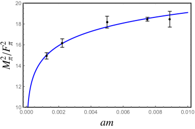
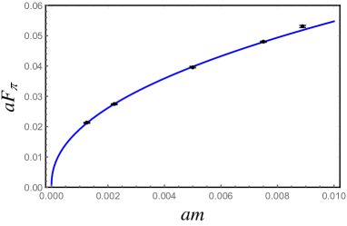
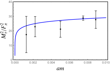
Figure 1: Representation of the 4-ensemble fit reported in the rightmost column of Table 1. The upper left-hand plot shows $M_{\pi}^{2}/F_{\pi}$ as a function of $am$, the upper right-hand plot shows $aF_{\pi}$, and the lower plot shows $M_{\tau}^{2}/F_{\pi}^{2}$.

Using the fit results from Table 1 we can infer some additional tree-level parameters of dChPT, or combinations thereof. The results for these derived quantities are collected in Table 2. First,

$$a\hat{f}_{\pi} = (d_{0}d_{2})^{\frac{1}{1+\gamma_{*}}}\ ,$$ (24)

$$a\hat{B}_{\pi} = {1\over 2}\,d_{0}^{\frac{2}{1+\gamma_{*}}}d_{2}^{\frac{1-\gamma_{*}}{1+\gamma_{*}}}\ .$$

As can be seen from Tables 1 and 2, the well-determined parameters are $\gamma_{*}$ and $\hat{B}_{\pi}$. These are the parameters that control the mass dependence; whereas $\hat{f}_{\pi}$, which has a much larger error, characterizes the massless theory. The values we find for $\gamma_{*}$, $a\hat{f}_{\pi}$ and $a\hat{B}_{\pi}$ agree well with the values found in Ref. Kutietal . The value of $\gamma_{*}$ is consistent with the earlier estimate of Refs. AIP1 ; AIP2 . Using also our results for $d_{3}$ allows us to obtain the ratio of the decay constants in the chiral limit, as well as the combination $c_{1}\hat{B}_{\tau}$ in units of $\hat{f}_{\pi}$,

$$\frac{\hat{f}_{\tau}}{\hat{f}_{\pi}} = 2\sqrt{\frac{3-\gamma_{*}}{d_{1}d_{3}}}\ ,$$ (25)

$$\frac{c_{1}\hat{B}_{\tau}}{\hat{f}_{\pi}^{2}} = \frac{1}{4}\,d_{3}\ .$$

Combining these two expressions, we also have

$$\frac{M_{\tau}(m=0)\hat{f}_{\tau}}{\hat{f}_{\pi}^{2}}=2\,\frac{\sqrt{c_{1}\hat{B}_{\tau}}}{\hat{f}_{\pi}}\,\frac{\hat{f}_{\tau}}{\hat{f}_{\pi}}\ ,$$ (26)

the value for which again is in good agreement with Ref. Kutietal .

	5 ens.	4 ens.
$a\hat{f}_{\pi}$	0.00049(22)	0.00065(27)
$a\hat{B}_{\pi}$	2.09(14)	2.15(14)
$\hat{f}_{\tau}/\hat{f}_{\pi}$	3.415(86)	3.427(88)
$c_{1}\hat{B}_{\tau}/\hat{f}_{\pi}^{2}$	0.708(77)	0.757(81)
$M_{\tau}(m=0)\hat{f}_{\tau}/\hat{f}_{\pi}^{2}$	5.75(32)	5.96(32)

Table 2: Derived quantities, see text.

To end this subsection, we return to the assumption that the lattice spacing $a$ is independent of $am$. Now that the fit parameters have been determined from a fit, we can test this assumption self-consistently, with a precision set by the errors of the fit. In particular, the fit parameters allow us to extract $a\hat{B}_{\pi}$ for each value of $am$ in the simulation separately, using Eqs. (3a) and (4),

$$a\hat{B}_{\pi,i}=\frac{(aM_{\pi,i})^{2}}{2am_{i}}\,e^{(\gamma_{*}-1)d_{1}M_{\pi,i}^{2}/F_{\pi,i}^{2}}\ .$$ (27)

Since $\hat{B}_{\pi}$ is by construction independent of $am$, this measures the dependence of $a$ on $am$. Using Eq. (27), and the results of the 4-ensemble fit, we find the values

$$a\hat{B}_{\pi,i}\ \in\ \{2.15(11)\,,\ 2.14(12)\,,\ 2.17(14)\,,\ 2.15(14)\,,\ 2.22(14)\}\ ,$$ (28)

for each of the fermion masses (23), respectively (the values obtained from the 5-ensemble fit are very close). In calculating the error in $\hat{B}_{\pi,i}$ we neglected the data errors for $M_{\pi}$ and $F_{\pi}$, and kept only the errors of (and correlation between) $\gamma_{*}$ and $d_{1}$, since the latter are much larger. We conclude that indeed $a\hat{B}_{\pi}$ is constant as a function of $am$, within errors. The values in Eq. (28) are consistent with the extrapolated value in Table 2.

In principle, we could have used any of the (dimensionful) LECs $a\hat{f}_{\pi}$, $a\hat{B}_{\pi}$, $a\hat{f}_{\tau}$ and $a^{2}c_{1}\hat{B}_{\tau}$ for this test. We chose to use the one that is most precisely determined from our fits, which is $a\hat{B}_{\pi}$. The values of the three other LECs are obtained by extrapolation to the chiral limit. As can be seen in Table 2, the precision of $\hat{f}_{\pi}$ is only 45%, and this also sets the precision with which we can determine $a\hat{f}_{\tau}$ and $a^{2}c_{1}\hat{B}_{\tau}$, cf.   Eq. (25).

$\chi^{2}$/dof	16.0/12	19.8/14	19.8/14
$p$-value	0.19	0.14	0.14
$\gamma_{*}$	0.934(19)	0.932(19)	0.932(19)
$\log{d_{0}}$	1.938(60)	1.943(59)	1.943(59)
$d_{1}$	0.251(26)	0.249(26)	0.249(26)
$\log{d_{2}}$	-16.70(94)	-16.64(93)	-16.65(93)
$d_{3}$	2.83(31)	2.84(31)	2.84(31)
$\log{C_{1}}$	$\star$	—	-13.9(1.1)
$\gamma_{1}$	$\star$	—	2.15(11)
$\log{C_{3}}$	-14.2(1.1)	-14.6(1.1)	—
$\gamma_{3}$	2.26(15)	2.15(10)	—
$\log{C_{4}}$	-14.1(1.2)	-13.89(95)	-13.53(95)
$\gamma_{4}$	1.94(19)	1.968(61)	2.003(51)
$\log{C_{6}}$	-48(23)	-64(11)	-64(11)
$\gamma_{6}$	-4.8(4.7)	-8.4(2.2)	-8.4(2.2)

Table 3: Results of fits to Eqs. (13), (22b) and (22c), using all 5 ensembles. A dash indicates a parameter that was omitted from the fit. The fit reported in the second column includes all parameters, but we do not quote a value for the parameters $\log{C_{1}}$ and $\gamma_{1}$ (entries indicated by a $\star$ symbol) since this fit could not resolve them. See text for further explanation.

IV.2 Fit including taste splittings

We now proceed to include the taste splittings, using, in addition to Eq. (13), also Eqs. (22b) and (22c). Only the masses of pions with tastes corresponding to the matrices $\Gamma_{i5}$ and $\Gamma_{ij}$ were reported in Ref. LSD2 , in addition to the mass of the $\Gamma_{5}$ pion (the Nambu–Goldstone pion), limiting us to consider only $\Delta_{A}$ and $\Delta_{T}$. With also $M_{\pi}$, $F_{\pi}$ and $M_{\tau}$, this gives us 5 data points per ensemble.

The second column of Table 3 reports the results of the fit that includes all 13 parameters occurring in tree-level staggered dChPT. We find $\chi^{2}/{\rm dof}=16.0/12$, for a $p$-value of 0.19. The first thing to notice is that the results for the “non-taste” parameters are in very good agreement with the results of the limited fit shown in Table 1.

While the fit includes all the dChPT parameters, we do not report any value for the parameters $\log{C_{1}}$ and $\gamma_{1}$. It turns out that, in effect, the $\chi^{2}$ function has a flat direction in the subspace spanned by these two parameters, leaving them undetermined. In order to understand this situation, consider first the parameters $\log{C_{6}}$ and $\gamma_{6}$. The negative mean values found for these parameters imply that $C_{6}E(\gamma_{6})=\exp[\log{C_{6}}+(4-\gamma_{6})v(m)]$ is negligibly small at the lighter masses, and becomes significant only for the highest one or two masses. A similar, but more dramatic, effect occurs in the case of the term $C_{1}E(\gamma_{1})$, which turns out to be significant for the highest mass only. This means that only one linear combination of $\log{C_{1}}$ and $\gamma_{1}$ (the one defined by the value of $v(m)$ at the largest mass) was constrained by the data, leaving the orthogonal linear combination undetermined.

Having seen that the existing data cannot resolve all the taste-splitting parameters, we also tried fits in which each operator occurring in Eq. (22) is omitted in turn. The 3rd and 4th columns of Table 3 report the results of the fits where we have set to zero $C_{1}$ or $C_{3}$, respectively. Both fits have an equally good $\chi^{2}$ and a $p$-value of 0.14. The fit with $C_{6}=0$ has $\chi^{2}=36.8$ while the fit with $C_{4}=0$ has $\chi^{2}=292$. Since both of them have a very low $p$-value, we do not report their results.

It is interesting that, by far, the worst fit is the one where we have set $C_{4}=0$. In other words, the data requires the presence of the $C_{4}E(\gamma_{4})$ term in the fit. This is nicely consistent with the taste splittings found in QCD, in the following sense. Due to the absence of the light scalar, the pattern of tree-level taste splittings in ordinary ChPT is much simpler, and corresponds to setting $E(\gamma_{i})=1$ everywhere in Eq. (22) AB . The actual taste splittings exhibit an almost equally spaced spectrum: the differences $\Delta_{A}-\Delta_{P}$, $\Delta_{T}-\Delta_{A}$, $\Delta_{V}-\Delta_{T}$ and $\Delta_{S}-\Delta_{V}$ are all roughly constant (independent of the fermion mass) and equal to each other. This approximate equality is explained by the dominance of the $C_{4}$ term. As can be seen in Eq. (22), its coefficient takes on the values 0, 1, 2, 3, and 4. Hence, in QCD, the constant displacement of the mass squared between adjacent tastes is given by $C_{4}$ itself. Returning to dChPT, the fact that $C_{4}$ cannot be omitted from the fit shows that, once again, the $C_{4}$ term is the most important one.

$\chi^{2}$/dof	6.1/9	6.2/9
$p$-value	0.73	0.72
$\gamma_{*}$	0.936(19)	0.936(19)
$\log{d_{0}}$	1.929(61)	1.928(61)
$d_{1}$	0.233(24)	0.233(24)
$\log{d_{2}}$	-16.18(86)	-16.18(86)
$d_{3}$	3.02(32)	3.01(32)
$\log{C_{1}}$	—	-12.3(2.9)
$\gamma_{1}$	—	2.49(91)
$\log{C_{3}}$	-13.0(3.0)	—
$\gamma_{3}$	2.50(92)	—
$\log{C_{4}}$	-12.7(1.8)	-12.3(1.9)
$\gamma_{4}$	2.16(53)	2.22(57)
$\log{C_{6}}$	-24(17)	-25(18)
$\gamma_{6}$	-0.2(3.6)	-0.3(3.7)

Table 4: Results of fits to Eqs. (13), (22b) and (22c), omitting the $am=0.00889$ ensemble. As in Table 3, a dash indicates a parameter that was omitted from the fit.

IV.3 Fits with 4 ensembles

The results reported in the previous subsection mean that some of the tree-level taste splitting parameters of dChPT acted as nuisance parameters in our fits: their presence is required in order to obtain a reasonably good fit, and yet they remain largely undermined. We have also explained how, in effect, these parameters serve to fit the taste-splitting data at the highest one or two masses, while having a very small, and often negligible, effect on the quality of the fit for the lighter masses.

This situation motivates us to also consider fits in which the highest mass, $am=0.00889$, is omitted. Due to severe numerical instabilities, we did not attempt a fit with all 13 parameters. The results of the fits with $C_{1}=0$ and with $C_{3}=0$ are reported in Table 4. Both of these fits now have a $p$-value slightly larger than 0.7. Figure 2 shows the results obtained for the taste splittings. (The results for $M_{\pi}$, $F_{\pi}$ and $M_{\tau}$ are visually the same as in Fig. 1.) The fit with $C_{6}=0$ has $\chi^{2}=10.2$, and a $p$-value of $0.49$, which by itself would be acceptable. However, it gives rise to $\log{C_{3}}=-5(8)$ and $\gamma_{3}=4.9(2.5)$, i.e., these parameters are much less well determined by this fit than by the fits reported in Table 4. Moreover, we regard the central value of $\gamma_{3}$ obtained in this fit as unphysical. As before, the fit with $C_{4}=0$ is inconsistent, having $\chi^{2}=117$.

Once again one can see that the values of the 5 “non-taste” parameters are essentially the same as in all previous fits. As for the taste-splitting parameters, while the mean values are consistent within error with the 5-ensemble fits, the errors themselves are significantly larger. In view of the high $p$-value of the 4-ensemble fits, the errors reported in Table 4 provide a more realistic estimate of current uncertainties in the data.

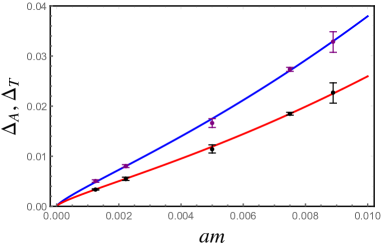
Figure 2: Representation of the taste splittings found in the 4-ensemble fits reported in Table 4. $\Delta_{A}$ is plotted in red, and $\Delta_{T}$ in blue. Left: fit with $C_{1}=0$. Right: fit with $C_{3}=0$.

V Conclusion

In this paper, we studied to what extent tree-level dilaton ChPT (dChPT) describes the pseudo-Nambu–Goldstone sector and the light singlet scalar state presented in the lattice data of Ref. LSD2 for the ${\rm SU}(3)$ gauge theory with $N_{f}=8$ fermions in the fundamental representation.

The simulations reported in Ref. LSD2 used staggered fermions, at 5 different fermion masses and one value of the gauge coupling, which, in turn, means a single lattice spacing. We showed that dChPT can be extended to incorporate the taste-breaking effects that are generally present with staggered fermions, arguing that, therefore, this provides a nice additional test of the applicability of dChPT to the data. We fitted data for the pion mass, the pion decay constant, the dilaton mass, and the two taste-split pion masses for which Ref. LSD2 provides data.

Even at tree level, staggered dChPT contains quite a few parameters, 13 in total. With only 25 data points, it is a challenge to determine all parameters. Indeed, attempting to fit all parameters simultaneously we found that two of them remain undetermined. The taste-breaking sector contains four operators, and discarding the pair of parameters associated with each of these operators in turn we found that some of the resulting fits are reasonably good when all 5 mass values are included. As we have explained, the highest-mass ensemble is particularly problematic when attempting to fit the limited available taste-splitting data. Omitting this ensemble, we find that the remaining 4 ensembles are well described by some of the fits in which one of the taste-breaking operators is omitted. Should data become available for the two pion tastes not considered in Ref. LSD2 , this would allow fitting also $\Delta_{V}$ and $\Delta_{S}$ in addition to $\Delta_{A}$ and $\Delta_{T}$. This would provide a more stringent test of dChPT, and may lead to a much better determination of the taste-splitting parameters.

With these caveats, we believe that dChPT provides a good explanation for the fermion-mass dependence of the taste splittings, which in this theory is very different from the analogous taste splittings in QCD, and for which standard staggered ChPT has not provided a convincing explanation. We do not claim that dChPT is the only possible explanation of these lattice data; it will be very interesting to test other low-energy approaches proposed in the literature BLL ; GGS ; CM ; MY ; HLS ; AIP1 ; AIP2 ; CT ; LSDsigma ; AIP3 , particularly if they can provide a valid description of the taste-breaking effects.

For the mass anomalous dimension we found $\gamma_{*}=0.936(19)$. We remind the reader that this value was obtained from data at a single lattice spacing, and does not include a continuum extrapolation. This value is in good agreement with the result of Ref. Kutietal , as well as with an earlier, more qualitative, analysis, based on the eigenmode number Annaetal . An interesting feature is that, in all cases where the anomalous dimensions $\gamma_{i}$ associated with the four-fermion taste-breaking operators were relatively well determined, their mean values turned out to be in the range of 1.9 to 2.5, or, in other words, about twice the value of the mass anomalous dimension. This result is intuitively appealing, if we remember that every four-fermion operator contains twice as many fermion fields as the mass operator.

Our fits also confirm that the simulations of Ref. LSD2 are in the “large-mass” regime, in which the theory shows approximate hyperscaling largemass . In Fig. 1 this is evident from the near-flatness of the ratios $M_{\pi}^{2}/F_{\pi}^{2}$ and $M_{\tau}^{2}/F_{\pi}^{2}$, with the strong downward curvature predicted by dChPT occurring mostly at smaller values of $am$ where no data points are available. Using

$$\frac{(3-\gamma_{*})m}{4c_{1}{\cal M}}=\frac{md_{1}}{d_{2}}\sim 4\times 10^{6}am\ ,$$ (29)

which even for the smallest value of $am=0.00125$ is of order $5\times 10^{3}$, we conclude that the left-hand side of Eq. (2) is indeed much larger than one for all masses in Eq. (23), thus confirming that these masses are in the large-mass regime.

A consequence of this is that also the values of $aF_{\pi}$ at the fermion masses (23), which range from approximately $0.02$ to $0.05$, are much larger than the chiral-limit value $aF_{\pi}(m=0)=a\hat{f}_{\pi}=0.00049(22)$. At the smallest fermion mass, the linear spatial volume in Ref. LSD2 is $L/a=64$, leading to $\hat{f}_{\pi}L\approx 0.03$. This implies that a much larger volume would be needed to study the theory in the $\epsilon$-regime. For comparison, at the smallest fermion mass in the simulation, $am=0.00125$, one has $F_{\pi}L\approx 1.3$, and $M_{\pi}L\approx 5.3$, so that the simulations of Ref. LSD2 are solidly in the $p$-regime, and finite-volume corrections are expected to be very small.

Recently, Ref. Kutietal20 reported tests of the SU(3) theory with two sextet (symmetric-representation) Dirac fermions in the $\epsilon$-regime. Random matrix theory (RMT) was used to determine the condensate in the massless limit, finding a value which is in agreement with another low-energy description AIP1 in which the tree-level dilaton potential takes on a different form from the one that follows from the power counting underlying dChPT. We stress, however, that dChPT does not provide any predictions whatsoever for these simulations, even if we disregard the fact that the theory under study contains fermions in a higher representation of the gauge group. The reason is that extrapolation of the $p$-regime data for $F_{\pi}$ to zero fermion mass using dChPT indicates that for the $\epsilon$-regime studies considered in Ref. Kutietal20 one has $F_{\pi}L\ll 1$ for the chosen combination of volume and fermion mass. As a result, the small-mass results are outside the range of applicability of dChPT. Were it possible to much enlarge the volume, while keeping $am\approx 0$, until eventually the condition $F_{\pi}(am\approx 0)L\approx\hat{f}_{\pi}L\approx 1$ would be satisfied, then, and only then, all measured quantities would have to agree with the predictions of dChPT, if indeed dChPT is the correct effective theory at low energy.

We comment that, as discussed in Ref. BGKSS , one can consider a partially-quenched setup where the sea fermions are kept in the $p$-regime and only the valence fermions are in the $\epsilon$-regime. In such a setup the dilaton expectation value is determine only by the mass of the sea fermions. This setup can provide for limited $\epsilon$-regime tests of dChPT on currently available ensembles.

Acknowledgments

We thank the LSD collaboration for providing the full covariance matrix for the spectroscopic data reported in Ref. LSD2 , and we thank Julius Kuti for discussions. MG’s work is supported by the U.S. Department of Energy, Office of Science, Office of High Energy Physics, under Award Number DE-SC0013682. EN’s work is supported by the U.S. Department of Energy, Office of Science, Office of High Energy Physics, under Award Number DE-SC0010005. YS is supported by the Israel Science Foundation under grant no. 491/17.

Appendix A The $m$ dependence of $\sqrt{8t_{0}}$

In QCD, $t_{0}$ is implicitly determined by the equation MLflow

$$t_{0}^{2}\left\langle E(t_{0},x)\right\rangle=0.3\equiv c_{0}\ .$$ (30)

(In SU($N$) gauge theories with $N\neq 3$, one needs an appropriate rescaling of the constant $c_{0}$, see for example Ref. TDflow .) Here

$$E(t,x)=\frac{1}{4}\,G_{\mu\nu}^{a}(t,x)G_{\mu\nu}^{a}(t,x)\ ,$$ (31)

where $G_{\mu\nu}^{a}(t,x)$ is the field strength of the flow field, which is subject to the boundary condition $G_{\mu\nu}^{a}(0,x)=F_{\mu\nu}^{a}(x)$, where $F_{\mu\nu}^{a}(x)$ is the field strength of the dynamical field, and with the convention that the classical action is $\frac{1}{4g^{2}}\int d^{4}x\,F_{\mu\nu}^{a}F_{\mu\nu}^{a}$.

In QCD, $E(t)$ admits a chiral expansion, from which it follows that BG

$$\left\langle E(t,x)\right\rangle=const.+O(m)+O(m^{2}\log(m))\ .$$ (32)

The $m$-independence of the leading term, and the (related) fact that logarithmic corrections occur only at NNLO, feeds into the chiral expansion for $t_{0}$, making it a particularly convenient quantity for scale setting in QCD.

Let us now consider a nearly conformal, confining theory. On dimensional grounds, the leading (operator) expression for $E(t,x)$ in the effective theory is

$$E(t,x)=C_{0}(t)e^{4\tau}\ ,$$ (33)

with $\tau$ is the dilaton field, and $C_{0}(t)$ an unknown function of $t$. Hence

$$\left\langle E(t,x)\right\rangle=C_{0}(t)e^{4v}\ ,$$ (34)

where $v=v(m)$ is the classical solution determined by Eq. (2). We see that, unlike in QCD, now the leading term depends on the fermion mass, because $v(m)$ does. Differentiating the relation

$$t_{0}^{2}C_{0}(t_{0})e^{4v(m)}=c_{0}\ ,$$ (35)

and using the approximate solution (5) valid for large $\frac{m}{c_{1}{\cal M}}$, gives

$$\frac{d\log(t_{0})}{d\log(m)}\ \sim\ -\frac{2}{1+\gamma_{*}}\frac{1}{1+{1\over 2}\frac{\partial\log(C_{0})}{\partial\log(t_{0})}}\ .$$ (36)

Naive hyperscaling, as determined on dimensional grounds, would suggest that the right-hand side of Eq. (36) be equal to $-\frac{2}{1+\gamma_{*}}$. The presence of the correcting factor on the right-hand side implies that $t_{0}$ does not have to obey the same hyperscaling relation as hadron masses and decay constants do in the large-mass regime largemass .

Moreover, the leading-order dependence of $\left\langle E(t)\right\rangle$ on $m$, coupled with our ignorance about the functional form of $C_{0}(t)$, implies that, unlike in QCD, we cannot write down a useful chiral expansion for $t_{0}$ in a nearly conformal theory. In a way, the situation is similar to that of the Sommer scale; one can empirically parametrize the (unknown) dependence of the Sommer scale on the quark mass. But, as for the Sommer scale, we do not have a theory-driven explicit expression to back up a particular expansion for the mass dependence.

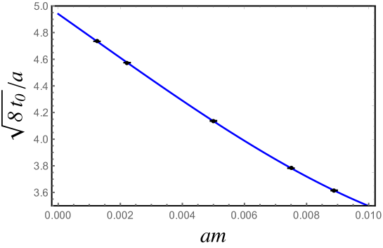
Figure 3: Fit of data for $\sqrt{8t_{0}}/a$ from Ref. LSD2 to a cubic polynomial.

It still interesting to fit the $am$ dependence of $\sqrt{8t_{0}}/a$, for which Ref. LSD2 also reported results with very small errors. Such a fit is purely “phenomenological,” because of the lack of a dChPT prediction for this dependence. We find that a fit of the data of Ref. LSD2 to a cubic polynomial in $am$,

$$R(am)=\sum_{n=0}^{3}a_{n}(am)^{n}$$ (37)

yields a statistically successful fit. This fit yields $\chi^{2}_{min}=0.78$, with one degree of freedom; the parameter values are given by

$$a_{0} = 4.9400(66)\ ,$$ (38)

$$a_{1} = -164.0(6.1)\ ,$$

$$a_{2} = -8(14)\times 10^{2}\ ,$$

$$a_{3} = 277(92)\times 10^{3}\ .$$

Figure 3 shows the fit. The value for $a_{0}$ is of interest, because it provides an estimate of $\sqrt{8t_{0}}/a$ in the chiral limit.

References

- (1)
- (2) T. DeGrand, Lattice tests of beyond Standard Model dynamics, Rev. Mod. Phys. 88, 015001 (2016) [arXiv:1510.05018 [hep-ph]].
- (3) D. Nogradi and A. Patella, Strong dynamics, composite Higgs and the conformal window, Int. J. Mod. Phys. A 31, no. 22, 1643003 (2016) [arXiv:1607.07638 [hep-lat]].
- (4) C. Pica, Beyond the Standard Model: Charting Fundamental Interactions via Lattice Simulations, PoS LATTICE 2016, 015 (2016) [arXiv:1701.07782 [hep-lat]].
- (5) B. Svetitsky, Looking behind the Standard Model with lattice gauge theory, EPJ Web Conf. 175, 01017 (2018) [arXiv:1708.04840 [hep-lat]].
- (6) T. Appelquist et al., Strongly interacting dynamics and the search for new physics at the LHC, Phys. Rev. D 93, no. 11, 114514 (2016) [arXiv:1601.04027 [hep-lat]].
- (7) T. Appelquist et al. [Lattice Strong Dynamics Collaboration], Nonperturbative investigations of SU(3) gauge theory with eight dynamical flavors, Phys. Rev. D 99, no. 1, 014509 (2019) [arXiv:1807.08411 [hep-lat]].
- (8) Y. Aoki et al. [LatKMI Collaboration], Light flavor-singlet scalars and walking signals in QCD on the lattice, Phys. Rev. D 96, no. 1, 014508 (2017) [arXiv:1610.07011 [hep-lat]].
- (9) T. Appelquist et al. [LSD Collaboration], Lattice simulations with eight flavors of domain wall fermions in SU(3) gauge theory, Phys. Rev. D 90, no. 11, 114502 (2014) [arXiv:1405.4752 [hep-lat]].
- (10) Z. Fodor, K. Holland, J. Kuti, D. Nogradi, C. Schroeder and C. H. Wong, Can the nearly conformal sextet gauge model hide the Higgs impostor?, Phys. Lett. B 718, 657 (2012) [arXiv:1209.0391 [hep-lat]].
- (11) Z. Fodor, K. Holland, J. Kuti, D. Nogradi and C. H. Wong, Can a light Higgs impostor hide in composite gauge models?, PoS LATTICE 2013, 062 (2014) [arXiv:1401.2176 [hep-lat]].
- (12) Z. Fodor, K. Holland, J. Kuti, D. Nogradi and C. H. Wong, The twelve-flavor -function and dilaton tests of the sextet scalar, EPJ Web Conf. 175, 08015 (2018) [arXiv:1712.08594 [hep-lat]].
- (13) Z. Fodor, K. Holland, J. Kuti and C. H. Wong, Tantalizing dilaton tests from a near-conformal EFT, PoS LATTICE 2018, 196 (2019) [arXiv:1901.06324 [hep-lat]].
- (14) Z. Fodor, K. Holland, J. Kuti and C. H. Wong, Dilaton EFT from p-regime to RMT in the -regime, arXiv:2002.05163 [hep-lat].
- (15) R. C. Brower, A. Hasenfratz, C. Rebbi, E. Weinberg and O. Witzel, Composite Higgs model at a conformal fixed point, Phys. Rev. D 93, no. 7, 075028 (2016) [arXiv:1512.02576 [hep-ph]].
- (16) T. Appelquist et al. [Lattice Strong Dynamics], Near-conformal dynamics in a chirally broken system, [arXiv:2007.01810 [hep-ph]].
- (17) M. Golterman and Y. Shamir, Low-energy effective action for pions and a dilatonic meson, Phys. Rev. D 94, no. 5, 054502 (2016) [arXiv:1603.04575 [hep-ph]].
- (18) M. Golterman and Y. Shamir, Effective field theory for pions and a dilatonic meson, PoS LATTICE 2016, 205 (2016) [arXiv:1610.01752 [hep-ph]]
- (19) M. Golterman and Y. Shamir, Effective pion mass term and the trace anomaly, Phys. Rev. D 95, no. 1, 016003 (2017) [arXiv:1611.04275 [hep-ph]].
- (20) M. Golterman and Y. Shamir, Large-mass regime of the dilaton-pion low-energy effective theory, Phys. Rev. D 98, no. 5, 056025 (2018) [arXiv:1805.00198 [hep-ph]].
- (21) T. Appelquist and Y. Bai, A Light Dilaton in Walking Gauge Theories, Phys. Rev. D 82, 071701 (2010) [arXiv:1006.4375 [hep-ph]].
- (22) T. V. Brown, M. Golterman, S. Krøjer, Y. Shamir and K. Splittorff, arXiv:1909.10796 [hep-lat].
- (23) C. N. Leung, S. T. Love and W. A. Bardeen, Aspects of Dynamical Symmetry Breaking in Gauge Field Theories, Nucl. Phys. B 323, 493 (1989).
- (24) W. D. Goldberger, B. Grinstein and W. Skiba, Distinguishing the Higgs boson from the dilaton at the Large Hadron Collider, Phys. Rev. Lett. 100, 111802 (2008) [arXiv:0708.1463 [hep-ph]].
- (25) Z. Chacko and R. K. Mishra, Effective Theory of a Light Dilaton, Phys. Rev. D 87, no. 11, 115006 (2013) [arXiv:1209.3022 [hep-ph]].
- (26) S. Matsuzaki and K. Yamawaki, Dilaton Chiral Perturbation Theory: Determining the Mass and Decay Constant of the Technidilaton on the Lattice, Phys. Rev. Lett. 113, no. 8, 082002 (2014) [arXiv:1311.3784 [hep-lat]].
- (27) M. Hansen, K. Langæble and F. Sannino, Extending Chiral Perturbation Theory with an Isosinglet Scalar, Phys. Rev. D 95, no. 3, 036005 (2017) [arXiv:1610.02904 [hep-ph]].
- (28) T. Appelquist, J. Ingoldby and M. Piai, Dilaton EFT Framework For Lattice Data, JHEP 1707, 035 (2017) [arXiv:1702.04410 [hep-ph]].
- (29) T. Appelquist, J. Ingoldby and M. Piai, Analysis of a Dilaton EFT for Lattice Data, JHEP 1803, 039 (2018) [arXiv:1711.00067 [hep-ph]].
- (30) O. Catà, R. J. Crewther and L. C. Tunstall, Crawling technicolor, arXiv:1803.08513 [hep-ph].
- (31) T. Appelquist et al. [LSD Collaboration], Linear Sigma EFT for Nearly Conformal Gauge Theories, Phys. Rev. D 98, no. 11, 114510 (2018) [arXiv:1809.02624 [hep-ph]].
- (32) T. Appelquist, J. Ingoldby and M. Piai, Dilaton potential and lattice data, Phys. Rev. D 101, no.7, 075025 (2020) [arXiv:1908.00895 [hep-ph]].
- (33) A. Bazavov et al. [MILC Collaboration], Nonperturbative QCD Simulations with 2+1 Flavors of Improved Staggered Quarks, Rev. Mod. Phys. 82, 1349 (2010) [arXiv:0903.3598 [hep-lat]].
- (34) M. Golterman, Applications of chiral perturbation theory to lattice QCD, arXiv:0912.4042 [hep-lat].
- (35) M. Golterman and Y. Shamir, arXiv:1910.10331 [hep-lat].
- (36) G. Veneziano, Some Aspects of a Unified Approach to Gauge, Dual and Gribov Theories, Nucl. Phys. B 117, 519 (1976); U(1) Without Instantons, Nucl. Phys. B 159, 213 (1979).
- (37) W. J. Lee and S. R. Sharpe, Partial flavor symmetry restoration for chiral staggered fermions, Phys. Rev. D 60, 114503 (1999) [hep-lat/9905023].
- (38) C. Aubin and C. Bernard, Pion and kaon masses in staggered chiral perturbation theory, Phys. Rev. D 68, 034014 (2003) [hep-lat/0304014].
- (39) O. Bär and M. Golterman, Chiral perturbation theory for gradient flow observables, Phys. Rev. D 89, no. 3, 034505 (2014) Erratum: [Phys. Rev. D 89, no. 9, 099905 (2014)] [arXiv:1312.4999 [hep-lat]].
- (40) A. Hasenfratz, A. Cheng, G. Petropoulos and D. Schaich, Reaching the chiral limit in many flavor systems, arXiv:1303.7129 [hep-lat].
- (41) M. Lüscher, Properties and uses of the Wilson flow in lattice QCD, JHEP 1008, 071 (2010) Erratum: [JHEP 1403, 092 (2014)] [arXiv:1006.4518 [hep-lat]].
- (42) T. DeGrand, Simple chromatic properties of gradient flow, Phys. Rev. D 95, no. 11, 114512 (2017) [arXiv:1701.00793 [hep-lat]].