VAT: Asymptotic Cost Analysis for Multi-level Key-Value Stores

Abstract

Over the past years, there has been an increasing number of key-value (KV) store designs, each optimizing for a different set of requirements. Furthermore, with the advancements of storage technology the design space of KV stores has become even more complex. More recent KV-store designs target fast storage devices, such as SSDs and NVM. Most of these designs aim to reduce amplification during data re-organization by taking advantage of device characteristics. However, until today most analysis of KV-store designs is experimental and limited to specific design points. This makes it difficult to compare tradeoffs across different designs, find optimal configurations and guide future KV-store design.

In this paper, we introduce the Variable Amplification–Throughput analysis (VAT) to calculate insert-path amplification and its impact on multi-level KV-store performance. We use VAT to express the behavior of several existing design points and to explore tradeoffs that are not possible or easy to measure experimentally. VAT indicates that by inserting randomness in the insert-path, KV stores can reduce amplification by more than 10x for fast storage devices. Techniques, such as key-value separation and tiering compaction, reduce amplification by 10x and 5x, respectively. Additionally, VAT predicts that the advancements in device technology towards NVM, reduces the benefits from both using key-value separation and tiering.

1 Introduction

Persistent key value (KV) stores [13, 2, 15, 17] are a central component for many analytics processing frameworks and data serving systems. These systems are considered as write-intensive because they typically exhibit bursty inserts with large variations in the size and type of data items [8, 31]. Consequently, over the last few years, KV stores have evolved to support many different applications and workloads [33]. There has been a number of new techniques that either optimize for different uses, e.g. write vs. read vs. scan or optimize certain aspects of system operation. As a result, this has increased the complexity of the KV-store design space to a point that it is unclear how each technique affects performance. Better understanding of KV-store design tradeoffs has the potential to improve both application performance and data serving infrastructure efficiency.

KV stores typically use at their core the write-optimized LSM-Tree [25] to handle bursty inserts and amortize write I/O costs. LSM-Tree [25] organizes data in multiple levels of increasing size (the size ratio of successive levels is known as growth factor). Each data item travels through levels until it reaches the last level. Data items generally move in batches from level to level with a merge/sort operation (compaction) that reorganizes data across levels. Each level is further physically organized into segments called sorted string tables (SSTables or SSTs). Each SST stores a non-overlapping and sorted subset of the key space.

Traditionally, such multi-level KV stores target Hard Disk Drives (HDDs) as the storage medium, because HDDs exhibit lower cost per bit of stored information. However, in HDDs, random I/O requests have a substantial negative effect on device throughput. For this reason, multi-level KV stores use large SSTs to always generate large I/O requests. Large SSTs have two important benefits: First, due to SST’s large size (in the order of MB), KV stores issue only large I/Os to the storage devices resulting in optimal HDD throughput. Second, they require a small amount of metadata for book-keeping due to their sorted and non-overlapping nature. SST metadata fit in memory and are only modified during compactions, thus they do not generate random I/Os in the common path. Therefore, multi-level KV stores are guaranteed to perform only sequential I/O to devices.

On the other hand, a significant drawback of the multi-level design is its high I/O amplification: The merge operation across levels results in reading and writing data many more times than the size of the data itself, resulting in traffic of up to several multiples of 10x compared to the dataset size [23]. Although amplification is so high, it still is the right tradeoff for HDDs: Under small, random I/O requests, HDD performance degrades by more than two orders of magnitude, from 100 MB/s to 100s KB/s.

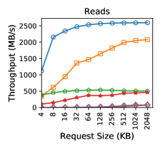
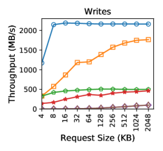
With the emergence of fast storage devices, such as NAND-Flash solid state drives (SSDs) and non-volatile memory devices (NVMe), the design space of KV stores has grown further. In modern devices, the device behavior is radically different under small, random I/Os: At relatively high concurrency, most of these devices achieve a significant percentage of their maximum throughput (Figure 1). At the same time, introducing some level of random I/Os can reduce amplification. Previous work [23, 26, 27, 7] has used this property of graceful device throughput degradation with random I/O to demonstrate the benefits of reducing I/O amplification and introducing various techniques, such as key-value separation and small SSTs with B+-tree indexing. These systems essentially draw a different tradeoff between device throughput and amplification. Therefore, modern storage devices dictate different designs for KV stores that draw a different balance between amplification and throughput to achieve higher performance in the insert-path, further increasing the complexity of the design space. Such designs can reduce the amount of data reorganization and therefore, they have the potential to both increase device efficiency and reduce CPU utilization.

Although these efforts derive from the original LSM design [25], they cannot be described by the LSM cost analysis, since it assumes that the system performs only large and practically fully sequential I/Os at the cost of performing a full read/write of two successive levels during each merge operation. Currently, there is no analysis that captures the tradeoffs between device throughput and amplification and reflects the cost for all these designs. The lack of such an analysis makes it more difficult to reason for tradeoffs across techniques and thus, navigate the design space and identify improved design points for new sets of requirements.

In this paper, we present VAT, a cost analysis for the insert-path that describes different techniques, such as leveling and tiering [19] compaction and performing key-value separation using value logs. VAT also captures the tradeoff of variable (as opposed to maximum) amplification vs. variable (as opposed to maximum) device throughput. We use VAT to derive optimal values for level growth factor, quantify the benefits of different design points, analyze tradeoffs, make projections and guide KV stores towards optimal design configurations.

Our VAT analysis, similar to the original LSM-Tree cost analysis [25], describes the operation of a multi-level system as a series of data transfers. Unlike the original analysis though, VAT introduces additional parameters for modeling different techniques as well as variable amplification and achieved device throughput. We use the VAT analysis to derive and solve a minimization problem that can quantify various aspects of KV-store designs, including the use of fast storage devices. In our analysis, we determine optimal values for the number of levels ($l$) and growth factor between levels ($f$), we examine differences across designs, and explore trends as device technology evolves. We find that by inserting randomness in the design, amplification drops by more than 10x, using a log can reduce amplification by 10x for small key-value size ratios of up to 1% and using tiering [19] instead of leveling decreases amplification by 5x, at the cost of read and scan operations.

Our main contributions are:

• We present VAT, an asymptotic cost analysis that captures data amplification in the insert-path for a wide collection of KV-store designs, including designs dictated by modern device technology. VAT can be extended to also capture additional design points in the future.

• We perform a comprehensive experimental analysis to show that VAT captures the behavior of four well-known KV-store systems, RocksDB [15], Kreon [27], BlobDB [14], PebblesDB [34], and that it accurately predicts e.g. the optimal level configuration for each design. Thus, VAT is a useful tool to understand tradeoffs between existing systems and configurations.

• VAT allows us to better understand: (a) the effects of device technology and randomness on I/O amplification and data reorganization cost, (b) optimal values for important parameters of existing KV stores and asymptotic trends, (c) tradeoffs between different design techniques, and (d) I/O and space amplification tradeoffs.

The rest of this paper is organized as follows: Section 2 briefly discusses necessary background, Section 3 presents VAT and the thought process behind the analysis, Section 4 presents our experimental methodology, Sections 5 presents our experimental results, and Section 6 discusses tradeoff analysis and VAT projections. Finally, Section 7 reviews related work and Section 9 concludes the paper. We also present supplementary detailed derivations for VAT and LSM-Tree analysis in appendices A and B.

Figure 1: FIO [3] throughput vs. request size, using iodepth 1 and 32, for three different device technologies: HDD (Western Digital Black Caviar 4 TB), SSD (Samsung 850 Pro 256 GB), and NVMe (Intel Optane P4800X 375 GB).

2 Background

A Log-Structured Merge (LSM) tree [25] is a multi-level data structure that optimizes for bursty inserts. The first level ($L_{0}$) is memory resident, whereas the rest of the levels are on the device. We assume that the LSM structure has $l$ levels and we denote by $S_{i}$ the size of level $L_{i}$ ($0\leq i\leq l$). In the original LSM paper [25] the levels have exponentially increasing sizes: For each $1<i\leq l$, $L_{i}$ contains $f$ times more data than the previous level $L_{i-1}$; where $f$ is the growth factor. Each level consists of a set of sorted string tables (SSTs) containing (key,value) pairs.

During an insert operation, LSM stores the key value pair is in the $L_{0}$ memory component. Periodically, the data of a level are flushed to the next (lower) level, to free up space in upper levels. This process is called compaction which produces excess read and write I/O traffic named amplification.

There are different ways to organize data across levels. In the leveling approach, each level organizes its key value pairs in non-overlapping SSTs. SSTs can be small and sequentially placed on the device [31], large(tenths of MB) and placed randomly [15], or small and random [27]. In leveling, a compaction merge-sorts SSTs from the upper level with overlapping SSTs from the lower level. Because of sorting, this incurs high I/O amplification and CPU overhead. In the tiering approach [19], there are overlaps in the key ranges of different SSTs within a level. When a compaction is triggered on a level, the SSTs residing on the level are sorted and moved to the next level, without performing any merging. Thus, tiering incurs significantly less I/O amplification but lower read performance than leveling due to overlapping of SSTs per level.

A set of systems [21, 23, 26, 27, 7] instead of storing values with keys in each level, they use KV separation. This technique appends values in a value log and only re-organize the keys (and pointers) in the multilevel structure. Note that the second technique incurs lower amplification than the first.

3 VAT: Variable Amplification-Throughput Analysis

In this section, we present the VAT asymptotic analysis to model different techniques of the multi-level KV-store design space and capture the variable amplification and achieved throughput tradeoff in fast storage devices. Specifically, VAT describes four categories of designs: leveling and tiering, with and without key-value separation (value log).

3.1 Modeling I/O traffic

The VAT basic equation, which we use to derive all subsequent relations, captures two major costs related to amplification in the insert-path: First, the cost that corresponds to the amount of excess I/O traffic generated during merge operations of two adjacent levels, the lower (larger) level and the upper (smaller) level. The basic equation measures this cost under the assumption that during a merge operation, the lower level is fully read and written. It is important to notice, that we refine this assumption in subsequent VAT equations. As a result, assuming the lower level is $f$ times larger than the upper level, the system reads and writes an excess of $f$ times more bytes, compared to the upper level. Second, the cost of data reorganization across levels: In a system with $l$ levels, each data item moves through all levels resulting in $l$ times excess traffic. We refer to these quantities of excess traffic as merge amplification and level amplification, respectively.

If $S_{0}$ is the size of the in-memory first level and $S_{l}$ is the size of the last level, then we can assume that the entire workload/dataset fits in (is equal to) $S_{l}$ and that all data will eventually move to the last level $S_{l}$. Then, $S_{l}/S_{i}$ is the total number of merge operations from $L_{i}$ to $L_{i+1}$, until all data reach $L_{l}$.

The basic equation measures the amount of I/O traffic $D$ produced until all $S_{l}$ data reach $L_{l}$:

$$D = \frac{S_{l}}{S_{0}}(S_{0})+2\sum_{j=1}^{S_{l}/S_{0}}((j-1)\bmod{f})\cdot S_{0}$$ (1)

$$+ \frac{S_{l}}{S_{1}}(2S_{1})+2\sum_{j=1}^{S_{l}/S_{1}}((j-1)\bmod{f})\cdot S_{1}$$

$$+ \ldots$$

$$+ \frac{S_{l}}{S_{l-1}}(2S_{l-1})+2\sum_{j=1}^{S_{l}/S_{l-1}}((j-1)\bmod{f})\cdot S_{l-1}$$

In equation (1), each sub-expression (row) captures the amplification of merging between two consecutive levels. For each such merge operation, there are two terms. The first term represents the data of the upper (smaller) level that have to be read and written during the merge operation, while the second term represents the data of the lower (larger) level.

For each level $L_{i}$, $0\leq i\leq l-1,$ each time one of the $S_{l}/S_{i}$ merge operations occurs, all data stored in $L_{i}$ are read and written, thus causing I/O traffic of size $2S_{i}$. This explains the first term that appears in each row. Also note that, in the first sub-expression for $L_{0}$ that resides in memory, the factor of $2$ is missing in the first term, indicating that we do not perform I/O to read data that are already in memory.

The second term captures the total amount of data that are read and written from $L_{i+1}$ in order to merge the overlapping ranges of $L_{i}$ and $L_{i+1}$. It uses the $\sum$ operator to express the fact that the merge operation happens multiple times as data flow through the system. It also uses the $\bmod$ operator to capture the fact that the size of the lower (larger) level grows incrementally up to $f$: in the first merge operation the lower level has no data (i.e., $j-1=0$); in the next merge, the lower level contains data equal to 1x the upper level; in each subsequent merge operation it contains data 2x, 3x, etc. of the data in the upper level. These data need to be read and written during merge, hence the factor of $2$ before the sum.

3.2 Modeling Variable Amplification and Device Throughput

Equation (1) assumes that the merge operation of two adjacent levels incurs the maximum possible amplification by reading and writing them in full. However, currently there are KV-store designs [26, 27, 23, 7, 36, 32] targeting fast storage devices (SSD, NVMe), which draw a different balance between amplification and device throughput. In particular, they reduce amplification by taking advantage of the property of fast storage devices to perform close to sequential throughput under random I/O pattern. VAT effectively captures this relationship between lower amplification at increased randomness and reflects the cost of various design decisions. It does so by introducing parameters $a$, $r$. The $a$ parameter models the impact of the SST size, the data organization technique, and the input, to amplification. In particular, $a$ expresses the percentage of the size of the lower level which is read and written during compaction. The $r$ parameter expresses the achieved device throughput and depends on the SST size and the degree of concurrency on the device. Both $a,r$ are in the range [0,1] (and $r\neq 0$). We call $a$ the merge amplification parameter and $r$ the achieved throughput parameter. Below we discuss how the SST size, data organization, and input affect $a$ and $r$.

SST Size: The use of small SSTs leads to a fine grained partitioned level with more SSTs per level. This allows to use techniques that reduce merge amplification significantly. For instance, reducing the SST size for cases where the input distribution is zipf can lead to reading a smaller percentage of the lower level at each compaction. This is because during a compaction, there is higher chance to find a hole in the key space of the lower level and thus choose to merge the SST of the upper level that fills that hole, therefore making the merge process cheaper in terms of I/O traffic produced.

Data organization: Leveling compaction [25] merges two levels keeping each level physically sorted in large chunks on the device. Therefore, the value of the merge amplification parameter $a$ is 1. Previous works have proposed various techniques [27, 32, 36, 34, 24] to lower the value of $a$. For instance, the use of compaction priorities in RocksDB [15] tries to change the order in which SSTs are merged to allow for merging, more frequently, SSTs to lower levels that are less full. This effectively reduces $a.$ Similarly, the use of an index [27] allows for smaller SSTs that are not necessarily contiguous on the device, therefore providing opportunities to reduce the amount of data amplification during merge operations. On the other hand, in tiering, merging happens only in the level that triggered the compaction, thus merge amplification $a$ is $0.$

Input: The input distribution, the ordering of keys and the percentage of updates, affect the overlap of keys in each pair of levels that will be merged. For instance, a uniform distribution where each (large) SST contains keys from the entire key space will result in maximum merge amplification ($a=1$), whereas a sorted input sequence of keys will result in $a=0.$

Determining $a$ and $r$ experimentally: Parameter $r$ depends mainly on the SST size. As a result, one can estimate the value of $r$ for a given KV-store design by using a micro-benchmark (e.g. FIO [3]) which simulates SST size and random I/O access pattern. Parameter $r$ value is the ratio of the measured throughput over the sequential. Note that $r$ also depends on the degree of concurrency: higher degrees of concurrency results in increased values for $r$. However, since most current systems achieve a high degree of concurrency, its effect on $r$ is more or less the same in all systems. As a result, we determine $r$ as a function only of the SST size and the device type. We calculate the value of $r$ as the percentage of the achieved throughput when random I/O operations of size equal to the target SST size are performed on the device (under high concurrency) over its sequential. Previous work [26, 27] has reported that KV stores are able to generate I/O queue depths of around 30, so we determine $r$ using a similar value. These values also agree with the experiments we performed with different KV stores in the context of this work.

Determining a realistic value for parameter $a$ is more involved. However, we observe that although the value of parameter $a$ depends on the KV-store design, it does not depend on the device technology: Although adaptive KV-store designs might be possible in the future, currently, KV stores do not adjust their main data structures and operations when using different devices. Thus, to determine the value of $a,$ we measure the amount of excess bytes during compaction with the lower levels by experimentally performing the following measurement. For each merge operation, we calculate:

$$a=\frac{MSST_{L}}{MSST_{U}(TSST_{L}/TSST_{U})}\,,$$

where $MSST_{L}$ and $MSST_{U}$ are the numbers of SSTs of the lower and the upper level, respectively, that participate in compaction, and $TSST_{L},$ $TSST_{U}$ are the numbers of total SSTs stored in the lower and upper level, respectively, at the time of merging. We then calculate the mean of all such values (over all the executed compactions) to get the estimated value for $a.$ Table 1 presents the result of the above measurement for the following systems: RocksDB [15], Kreon [27], BlobDB [14], and PebblesDB [34]. Typically, each KV store uses a specific growth factor $f,$ at around 10. We choose the growth factor $f=8$ since it is close to 10 and it is the growth factor that makes the capacity of the last level equal to the workload size. We discuss these values further in our results.

$f$	RocksDB	Kreon	BlobDB	PebblesDB
8	0.68	0.25	0.8	0

Table 1: Merge amplification $a$ for growth factor $f=8.$

3.3 The VAT Cost Analysis

In this section, we present the VAT cost analysis. We first provide the basic VAT analysis and then we present similar equations for different designs, like key-value separation with a value log and tiering.

Basic VAT Analysis:

VAT calculates the time $T$ to write the data of size $S_{l}$ (that fit in the last level) and the optimal time $T_{opt}$ as follows:

$$T=\frac{D}{r\cdot R_{opt}}\hskip 14.22636pt\mbox{ and }\hskip 14.22636ptT_{opt}=\frac{S_{l}}{R_{opt}}$$ (2)

$R_{opt}$ is the optimal device throughput and $r\cdot R_{opt}$ is the achieved device throughput (recall that $r$ is in the range (0,1]). The optimal time to write the data can be expressed as the ratio of the minimum amount of data $S_{l}$ to be written with the maximum possible throughput $R_{opt}$, as would e.g. be the case for appending all data in a log file.

Now, we derive the base VAT analysis. By inserting $a$ in Equation (1) we get:

$$D = \frac{S_{l}}{S_{0}}(S_{0})+2a\sum_{j=1}^{S_{l}/S_{0}}((j-1)\bmod{f})\cdot S_{0}$$ (3)

$$+ \ldots$$

$$+ \frac{S_{l}}{S_{l-1}}(2S_{l-1})+2a\sum_{j=1}^{S_{l}/S_{l-1}}((j-1)\bmod{f})\cdot S_{l-1}$$

Note that $S_{l}/S_{l-i}=f^{i}$ (assuming $f$ is constant). Using this, we perform arithmetic transformations to analyze the sum (see Appendix A.1):

$$D=S_{l}(2l-1-al+afl)$$ (4)

Ideally, we would like a KV-store design to minimize the quantity $\frac{T}{T_{opt}}$ and achieve a time as close to optimal as possible. For this reason, VAT focuses on the following minimization problem: $\displaystyle\min_{\begin{subarray}{c}0\leq a\leq 1\\ 0<r\leq 1\end{subarray}}\frac{T}{T_{opt}}$. Using Equation (4), we get:

$$\frac{T}{T_{opt}}=\frac{2l-1-al+afl}{r}$$ (5)

Considering $a$ and $r$ are fixed values for a given design, Equation (5) expresses $T/T_{opt}$ as a function of $l$ and $f$. So, by studying the minimization problem, we gain insight in the tradeoff between the number of levels and the growth factor.

VAT for key-value separation:

We now apply the VAT analysis (presented above) to express key-value separation using a value log. Denote by $K_{i}$ and $V_{i}$ the total size of keys and values, respectively, of each level $L_{i}.$ Note that each SST now stores only keys and thus its level is equal to $K_{i}.$ However, in our equations below, we let $S_{i}=K_{i}+V_{i}.$ The value log contains all the key-value pairs stored in the system, so its size is $S_{l}.$ Following a similar approach as above, we express the total I/O traffic as:

$$D = \frac{K_{l}}{K_{0}}(K_{0})+2a\sum_{j=1}^{K_{l}/K_{0}}((j-1)\bmod{f})\cdot K_{0}$$ (6)

$$+ \ldots$$

$$+ \frac{K_{l}}{K_{l-1}}(2K_{l-1})+2a\sum_{j=1}^{K_{l}/K_{l-1}}((j-1)\bmod{f})\cdot K_{l-1}$$

$$+ S_{l}$$

The last term $S_{l}$ in Equation (6) accounts for appending the entire dataset in the value log. Let $p=K_{l}/V_{l}$. Then, $p$ is typically a small constant ($0<p<1$). Using Equations (2), we get (see Appendix A.2 for the derivations):

$$D = K_{l}\Big{(}2l-1-al+afl\Big{)}+S_{l}$$ (7)

$$\frac{T}{T_{opt}} = \frac{p(2l-1-al+afl)+p+1}{r\cdot(p+1)}$$ (8)

KV stores are used to support diverse workloads [33], where key and value sizes may differ within a wide range: in typical workloads, keys are a few tens of bytes, whereas values vary from similar sizes to a few KB of data (thus resulting in values of $p$ much smaller than $1$). Therefore, in our evaluation we examine various data points where key to value size ratio spans the range from 1 to 0.01.

Note that for small values of $p$, e.g. close to 0.01, the ratio in Equation (8) is much smaller (the numerator is smaller than the denominator) than that in Equation (5). This way, VAT shows that using key-value separation with a value log has a significant benefit in terms of incurred amplification.

VAT for tiering:

In tiering compaction, excess traffic during merge operations includes only reading and writing the data in $L_{i}$ (and not $L_{i+1}$ as in leveling). Therefore, $a=0$. By setting $a=0$ in Equation (5), we get the equations for tiering:

$$\frac{T}{T_{opt}} = \frac{2l-1}{r}=\frac{2\log_{f}C-1}{r}\,,$$ (9)

where $C=S_{l}/S_{0}=f^{l}$ (and therefore $l=\log_{f}C$).

Equivalently to Equation (6), to model the cost of tiering with key-value separation, we slightly modify the analysis above to only consider keys ($K_{l}$) instead of both keys and values ($S_{l}$).

$$\frac{T}{T_{opt}}=\frac{p(2l-1)+p+1}{r\cdot(p+1)}=\frac{p(2log_{f}C-1)+p+1}{r\cdot(p+1)}$$ (10)

These equations express the fact that tiering does not depend on the size of the next level and therefore, on $a,$ which expresses excess bytes related to the next level. Consequently, tiering cannot benefit as much as leveling from emerging device technologies in the insert-path.

VAT Equations:

In summary, the VAT analysis can describe different designs, in terms of cost for the insert-path, as shown in Table 2.

	no log	log
VAT $T/T_{opt}$	$\frac{2l-1-al+afl}{r}$	$\frac{p(2l-1-al+afl)+p+1}{r\cdot(p+1)}$

Table 2: VAT equations for the minimization problem $T/T_{opt}$.

4 Experimental methodology

In our evaluation, we examine two main aspects of VAT:

• How accurately VAT can model the behavior of different techniques. We use four existing KV-store systems to examine how accurately VAT can model different points in the design configuration space: RocksDB [15], Kreon [27], BlobDB [14], and PebblesDB [34].

• How VAT can help understand tradeoffs between different design points. For this purpose we quantify the benefits of different designs, present observations on their asymptotic behavior and make projections as device technology improves.

The real systems we use in our measurements incur significant complexity, especially systems such as RocksDB that is used extensively in real-life applications and support many different modes of operation. Next, we discuss how we modify or configure each system for our purposes.

RocksDB:

RocksDB by default performs leveling compaction with values in-place with keys. However, RocksDB can also operate in different modes and use several techniques that try to reduce amplification in a non-asymptotic manner. Given that VAT models asymptotic behavior, we make a number of modifications to RocksDB configuration and code to disable certain non-asymptotic optimizations: We modify RocksDB to move all SSTs of intermediate levels to the last level upon termination, to better approximate steady state operation with large workloads, similar to what VAT models. We disable the Write Ahead Log (WAL) mechanism, since we measure the I/O traffic produced solely by compactions. We configure RocksDB to perform leveling compaction with different growth factors. We use the default RocksDB configuration for memtables (2x64MB) and $L_{0},L_{1}$ size (256MB) with a maximum of 4 SSTs in $L_{0}$. Therefore, only levels greater or equal to $L_{1}$ exhibit the prescribed growth factor with respect to the previous level. Essentially, value $l$ in the asymptotic analysis of LSM and VAT corresponds to $l+1$ in RocksDB, since in the cost model, levels $L_{0}$ and $L_{1}$ also obey the growth factor $f$.

Kreon:

Kreon uses a value log for key-value separation and organizes the metadata using a multi-level index. We use a 256MB $L_{0}$, which is more than enough to hold the metadata of a 16GB workload in memory. Kreon by default stores 200 keys per SST. With a uniform distribution, merge amplification $a$ is close to 1. However, by only decreasing the number of keys stored per SST down to 4, resulting in more SSTs per level, thus a more fine grained partitioned level, the system achieves lower merge amplification with $a=0.25.$

BlobDB:

BlobDB is a wrapper of RocksDB that employs key-value separation using a value log. It stores values in blobs (log files) and keys along with metadata in RocksDB’s LSM index. We use the same configuration with RocksDB.

PebblesDB:

PebblesDB is built on top of LevelDB [17] and features tiering compaction. We perform similar modifications to better approximate steady state operation. PebblesDB uses the notion of guards. Each guard has a set of associated SSTs and divides the key space (for that level) into disjoint units. Guards within a level never have overlapping key ranges. The growth factor in PebblesDB is the number of SSTs in a guard that triggers the compaction.

Workload:

In our measurements we use a single YCSB [29] thread to produce a workload of 16 million key-value pairs with a value size of $\approx$ 1 KB (1079 bytes). We generate uniformly distributed keys over a configurable key universe. We limit the key universe to only contain 3-byte keys and we generate all 16 million keys in the full range. To do this, we sort the keys and then we use a stride equal to the ratio of the key universe range over the number of keys in each SST, to cover the full key universe in a uniform manner, for every SST that is generated. We run our experiments using a single database on a Samsung SSD 850 PRO 256GB. For each run, we vary the growth factor and let the KV stores spawn the corresponding levels.

We calculate I/O amplification as follows. We measure I/O traffic externally to the KV stores, using iostat to ensure we capture all device traffic. We disable the use of the buffer cache so that all traffic to the devices is visible to iostat. We measure the read and write traffic in bytes during each experiment. We calculate the amplification ratio by dividing I/O traffic with the size of the YCSB dataset ($(1079+3)\cdot 16M$). For VAT, we set $r=1,$ for RocksDB, BlobDB and PebblesDB since they use large SSTs. Kreon produces 8KB requests. We used FIO [3] and measured the achieved performance with 8KB requests to be $r=0.91$ on the NVMe device we used for the experiments. Equation 11 shows that $\frac{T}{T_{opt}}$ can also be expressed as a ratio of bytes:

$$\frac{T}{T_{opt}}=\frac{D/(r\cdot R_{opt})}{S_{l}/R_{opt}}=\frac{D}{r\cdot S_{l}}$$ (11)

5 VAT on several KV-store designs

In this section, we use measurements from the four KV stores in our experimental setup to show that VAT captures the behavior of different design points and is able to suggest the optimal level configuration for each technique. Figure 3 summarizes our experimental results, which we discuss below.

(a) $r=1$, $C=1000$

(b) $a=1$, $C=1000$

Figure 2: (a) VAT cost ratio ($T/T_{opt}$) for optimal throughput ($r=1$) and different values of merge amplification $a.$ (b) VAT cost ratio at maximum merge amplification ($a=1$) and different values of achieved device throughput $r.$

(a) RocksDB

(b) Kreon

(c) BlobDB

(d) PebblesDB

Figure 3: VAT models for different KV-store designs and actual measurements.

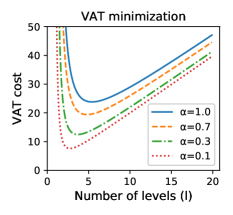
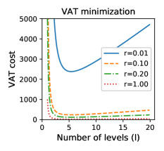
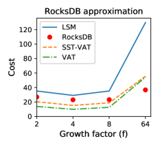
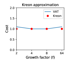
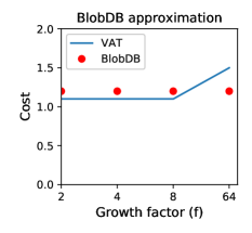
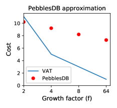
Figure 3(a) shows the cost ratio $\frac{T}{T_{opt}}$ with an increasing number of levels for leveling without a value log as calculated with VAT and as measured with RocksDB. We also include the cost as calculated by LSM-Tree analysis. We see that VAT is close to the actual measurements.

In addition, RocksDB performs compactions between two levels $L_{i}$ and $L_{i+1}$ on a per-SST basis. Therefore, a compaction in RocksDB does not necessarily merge all SSTs of $L_{i}$ to $L_{i+1}.$ This results in all levels being continuously almost full. VAT expresses this behavior as follows (where $B$ is equal to the SST size):

$$D =\frac{S_{l}}{S_{0}}\frac{S_{0}}{B}B+2a\Big{(}\sum_{i=1}^{f\frac{S_{0}}{B}}\frac{i}{\frac{S_{0}}{B}}+f\big{(}\frac{S_{l}}{S_{0}}\frac{S_{0}}{B}-f\frac{S_{0}}{B}\big{)}\Big{)}B$$

$$+\cdots$$

$$+\frac{S_{l}}{S_{l-1}}\frac{S_{l-1}}{B}2B+2a\Big{(}\sum_{i=1}^{f\frac{S_{l-1}}{B}}\frac{i}{\frac{S_{l-1}}{B}}+f\big{(}\frac{S_{l}}{S_{l-1}}\frac{S_{l-1}}{B}-f\frac{S_{l-1}}{B}\big{)}\Big{)}B$$ (12)

By performing calculations (see Section A.4), we get:

$$D =S_{l}\Big{(}2l-1+\frac{aflB}{S_{l}}+2afl-af\big{(}\frac{1-\frac{1}{f^{l}}}{1-\frac{1}{f}}\big{)}\Big{)}$$ (13)

Figure 3(a) includes this extension as SST-VAT and shows that it tracks RocksDB behavior even closer compared to VAT.

Figure 2(b) shows how VAT captures the effect of designs that exhibit a reduced value for $a$ (reduced amplification) resulting in lower $r$ (reduced device throughput) as well. Kreon uses a value log and small-size SSTs with an index. Small SSTs allow for a reduced $a.$ At the same time, Kreon exhibits a lower $r$ due to the randomness introduced from small SSTs. With modern storage devices, experiments showed that $r$ for Kreon is around 0.91, which is close to the optimal value of 1. Figure 3(b) shows that the measured values from Kreon are close to the cost calculated by VAT. We note that LSM [25] cost analysis does not describe designs similar to Kreon, therefore, we do not include a curve from LSM-type analysis.

BlobDB tries to reduce amplification by also using a value log and merging only metadata (keys and pointers) during compaction. VAT modeling for leveling with a value log successfully captures this behavior, as shown in Figure 3(c). Amplification is reduced significantly because of value separation and the use of small keys in our workload (default for YCSB).

BlobDB exhibits a value of 0.8 for $a,$ compared to 0.68 in RocksDB (Table 1). Although both systems use leveling, the use of the value log in BlobDB results in more keys per SST compared to RocksDB where SSTs contain both keys and values. As a result, one SST in BlobDB, typically overlaps with more SSTs of the next level, resulting in a higher value for $a.$ At the same time, both systems achieve the same device throughput, as they use similar size SSTs.

In Figure 3(d) VAT models tiering and PebblesDB that uses a form of tiering. VAT indicates that a larger growth factor should result in in less amplification. However, we note that PebblesDB does not decrease amplification with the same rate as VAT does because it is not a pure tiering system. The reason for this is that PebblesDB tries to improve read behavior as follows. To reduce the number of SSTs that need to be examined during a read operation, it maintains overlapping SSTs only within guards which results in higher amplification during compactions. Therefore, although VAT captures the cost of “pure” tiering, PebblesDB exhibits higher cost in the insert-path. Both exhibit a reducing trend as growth factor increases, as is expected for amplification in systems that use tiering.

6 Tradeoff analysis

In this section, we use VAT to examine tradeoffs across different design points and make additional observations.

The effects of randomness:

Figure 2(a) shows the curves of base VAT for different values of $a$ while maintaining optimal throughput with $r=1$. As $a$ decreases, indicating systems that make use of randomness to reduce amplification, the optimal number of levels that minimize amplification decreases as well. Minimum amplification drops from about 25x to less than 10x, when $a$ decreases from 1.0 to 0.1. Therefore, techniques that make use of randomness to reduce $a$ can lead to increased KV-store efficiency. Secondarily, we see for all values of $a,$ an inappropriate number of levels (small or large) leads to very high amplification, exceeding 50x for small numbers of levels, which implies large growth factors.

Optimal growth factor:

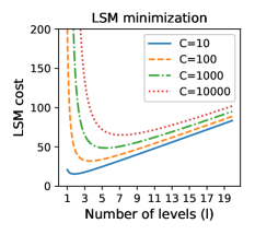
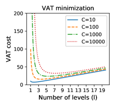
The analysis in Appendix A.3 shows that the growth factor between any two consecutive levels must either be the same or converge to the same value. Also, we note that the optimal growth factor is constant regardless of the dataset size. Therefore, as data grows, both VAT and LSM dictate that to minimize amplification we have to increase the number of levels, as opposed to increasing their relative size. Figure 6(a) and Figure 2(a) plot amplification as a function of the number of levels for different values of $a$ and $C$. In both cases, the part of each curve to the left of the optimal number of levels is more “steep” than the part of the curve to the right. This means that to store the same amount of data in multi-level designs that perform leveling, and if it is not possible to use the optimal number of levels, e.g. because of other considerations, it is preferable in terms of amplification to err towards using a larger number of levels (and lower $f$) than the opposite.

Space amplification matters as well:

Many systems choose larger than optimal growth factors to improve space efficiency. If we assume that intermediate levels are usually full with updates that will be garbage collected during compactions, then intermediate levels incur space amplification, which increases device cost. Space amplification (excluding the size of user data) can be roughly calculated as $\frac{S_{0}+\ldots+S_{l-1}}{S_{l}}=\frac{1}{f}+\ldots+\frac{1}{f^{l}}.$ Using $f=4$ results in space amplification larger than 25%, which might be considered excessive, especially for expensive storage devices, such as SSDs and NVMe. If we use $f=10$ then space amplification drops to about 10%. VAT shows that for $a=1$, $\frac{T}{Topt}=32$ for $f=10$ and $\frac{T}{Topt}=23.91$ for $4$, so increasing $f$ from $4$ (close to optimal) to $10$ makes amplification in the insert-path worse by about 1.33x, which is an acceptable cost for reducing space amplification by 2.5x (from 25% down to 10%). Therefore, VAT allows system designers and users to tune the system design or configuration.

Single tier for future fast storage devices:

As technology improves, devices will be able to achieve maximum throughput for even smaller block sizes, e.g. about 256 bytes for recent NVM devices [18]). This will allow KV stores to use even smaller SSTs, further decreasing the value of merge amplification $a.$ If we assume that $a$ can become 0, this would result in KV stores with a single level, as indicated by Equation 14:

$$\frac{T}{T_{opt}}=\frac{2l-1-al+afl}{r}\xRightarrow[\text{$r=1$}]{\text{$a=0$}}\frac{T}{T_{opt}}=2l-1$$ (14)

However, we should note that having a value of $a=0$ may not be possible for arbitrary key sizes, unless devices become truly byte addressable and are used as such.

(a) $f=10$, $C=1000$

(b) $p=1\%$, $r=1$, $C=1000$

Figure 4: (a) Amplification benefit of using a value log compared to placing the values in place. (b) Amplification benefit of tiering compared to leveling compaction.

Key-Value separation on future devices:

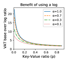
Figure 4(a) shows that using a value log brings significant benefits when the key-value size ratio is small, about $p=1\%.$ In addition, the value of $a$ affects the benefits of using a value log. VAT shows in Figure 4(a) that for values $a\geq 0.3$ the benefit is more than 10x. However, as device technology evolves, it allows for optimal device throughput with smaller unit size, and $a$ can reduce, e.g. to $0.25$ for certain configurations in Kreon (Table 1). Using Equation 15 VAT shows that the benefit of using a log as $a$ approaches $0$ is given by:

$$\frac{\frac{2l-1-al+afl}{r}}{\frac{p(2l-1-al+afl)+p+1}{r\cdot(p+1)}}\xrightarrow[\text{$l=1$}]{\text{$a=0$}}\frac{p+1}{2p+1}$$ (15)

So for any key-value size ratio Equation 15 shows that KV separation is actually worse that placing the values in-place with keys, especially when introducing the extra cost of garbage collection (see Section 8).

(a) $p=1\%$, $r=1$, $C=1000$

(b) $r=1$  $C=1000$

Figure 5: (a) VAT for tiering. (b) VAT for tiering with values in log.

Does tiering still make sense with future devices?

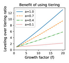
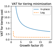
In Figure 5(a), VAT shows that when using tiering with in-place values, one should probably use a growth factor $f$ of around 10, which is the point of diminishing returns for amplification. After $f=10,$ amplification reduces less, while read operations continue to become slower. VAT also expresses the fact that with tiering, throughput does not depend on merge amplification. Thus, tiering cannot benefit from improved device technology and the ability to reduce $a.$ Furthermore, Figure 4(b) shows that the benefit of tiering reduces as merge amplification decreases: As compactions become cheaper, i.e. $a$ reduces, the benefit of tiering becomes smaller.

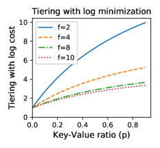
Tiering techniques so far have placed values along with keys [19] without using a log. In Figure 5(b) VAT shows that tiering with a log can be a valid approach for small values of $f$, which do not reduce read performance significantly and for small $p$ ratios, up to $10\%$. However, in this case, Figure 4(a) shows that the amplification benefit is also significant for leveling with a value log, about 10x. In addition, leveling with a value log has better scan performance compared to tiering with a value log. Therefore, for small $p$ ratios, it is preferable to use a value log with leveling.

7 Related Work

In this section we first present a taxonomy of various KV-store designs and then relate this space to VAT.

Taxonomy:

Table 3 provides a high-level taxonomy of existing systems that to some extend have tried to take advantage of device properties and improve performance, similar to what VAT models. In this taxonomy, we use three dimensions:

Size and placement of SSTs: The SST size used to organize data within each level and their placement on the device is typically large. Large SSTs guarantee maximum device throughput, eliminating the effects of the I/O pattern (sequential or random) and metadata I/Os, as metadata is small and fits in memory. Small and sequentially placed SSTs on the device [31] can achieve the same goal of maximum device throughput. This results in high I/O amplification but improves read performance at the expense of maintaining more metadata. Emerging device technologies allow using small SSTs with random placement which introduces randomness but has the potential to reduce I/O amplification [27]. This approach is suitable for devices where random I/O throughput degrades gracefully compared to sequential I/O throughput.

Logical level organization: Keys in each level are logically organized either fully or partially. Full organization keeps the key space in fully sorted, non-overlapping SSTs. Full organization is usually done with leveling compaction [25, 15, 35, 4, 11, 38, 16, 21, 23, 7]. However, B+-tree indexes have also been used to either optimize reads and scans [31] or reduce amplification [27]. Partial organization maintains the key space in overlapping units, e.g. in the form of tiering compaction [36, 10, 28, 24, 20] which reduces merge amplification at the cost of reduced read and scan performance.

Value location: Finally, values can be placed either in-place with keys or in a separate value log. Typically, values are stored in-place because this results in optimal scan behavior at the expense of increasing amplification due to value movement during merge operations. Previous work has proposed techniques [7, 21, 23, 26, 27] that store values in a log, reducing amplification significantly, relying on modern devices to alleviate the impact on scan performance.

VAT is able to describe the design points within this taxonomy and quantify tradeoffs across these designs, as device technology improves.

	SST size,	Organi-	Value
	placement	zation	placement
LSM[25], RocksDB[15],	Large	Full	In-place
Locs[35], Dostoevsky[11],
Triad[4], Mutant[38],
bLSM[31], cLSM[16]
Atlas[21], WiscKey[23],	Large	Full	Log
HashKV[7]
LSM-trie[36], Monkey[10],	Large	Partial	In-place
SifrDB[24], Novelsm[20]
PebblesDB[28]
Kreon[27]	Small	Small	Log
$B^{e}$-tree[5]	Small	Full	In-place

Table 3: Taxonomy of the main approaches to design KV stores in three dimensions.

LSM-Tree cost analysis:

The LSM-Tree analysis [25] quantifies the tradeoff between device throughput and amplification and shows that asymptotically it is better to increase device throughput at the cost of high amplification for HDDs. VAT generalizes this analysis to a much broader collection of KV-store design techniques, which includes those that are dictated by modern device technology.

Merge and level amplification are competing quantities: As we see in Figure 6(a), for a given amount of data, if we reduce the number of levels $l$, we have to increase the growth factor $f$ between two consecutive levels. Similarly, reducing the growth factor $f$, results in increasing the number of levels $l$. Therefore, in a proper LSM design there is a need to balance $l$ and $f$ to minimize the total I/O amplification. The LSM-Tree analysis [25] solves this minimization problem in two cases: (1) when the size ratio of the entire dataset to main memory is constant and (2) when the sum of the capacities of all levels is constant. In Appendix B.1, we use the equations in [25] to solve the minimization problem without applying the formula simplification used in [25] that minimizes the total I/O amplification.

(a) LSM

(b) VAT, $a=r=1$

Figure 6: (a) Amplification vs. number of levels as a result of minimizing the LSM cost for various $C=\frac{Workload~{}size=S_{l}}{DRAM~{}size=S_{0}}$ ratios. (b) Amplification vs. number of levels as a result of minimizing VAT cost for various $C$ ratios.

Alternative KV-store cost analyses:

The authors in [22] propose a model that calculates the cost of write and read amplification in multi-stage log-structured KV-store designs, offline without the need to run long experiments. Their model takes into account redundancy (duplicate keys) and uses this to estimate overheads based on unique keys. They find that the proposed approach can accurately model the performance of LevelDB and RocksDB and they show how the model can be used to improve the insert cost in both systems. VAT shares the goal of modeling write amplification in multi-stage KV stores (see Figure 6(b)), however, aims to capture the behavior of the underlying device technology (parameter $r$) and also the impact of merge amplification (parameter $a$) of several design factors. VAT does not take into account redundancy in the key population but rather aims to capture asymptotic behavior of different designs and approaches. Our results show that VAT can describe several existing techniques and design tradeoffs.

MonkeyDB [10] and Wacky [12] propose and use models to explore tradeoffs in the design of multi-level KV stores. They focus on optimizing the use of memory for different aspects of KV stores. Wacky uses this analysis to search analytically a broad space of merge policies and other parameters with the goal to identify the parameters that best match a given workload. The model of Wacky takes into account both the write and read path and aims to optimize the system for insert, read, and scan operations. Unlike Wacky, VAT focuses on expressing asymptotically write amplification and takes into account the impact of device technology. VAT allows us to explore tradeoffs across design points in the configuration space, including improving device technology.

8 Discussion

In this section we make various observations extracted from our analysis and evaluation process to provide further insight. We believe that VAT can be generalized further to (a) take into account additional important resources and (b) express the cost of additional operations, in addition to insert path amplification. For instance, VAT can consider read path amplification, space amplification, optimal unit of transfer (write, read), etc. Next, we discuss some of these in more detail.

Unit of transfer in compaction:

In Section 5 we briefly discuss that RocksDB performs compactions in a per-file manner which results in lower tail latency but increased amplification. Tail latency is an important metric for data serving systems that significantly affects the perceived quality of the system. In KV stores, it is desirable that the system does not block for long periods when reorganizing data, especially given the volume of data stored in lower levels. VAT in Section 3, expresses compactions in a “stepped” approach, where each compaction merges the entire $level_{i}$ in $level_{i+1}.$ This approach, although simpler to express analytically, it describes a system where a single compaction might require that several hundreds of GBs are moved on the device. This process will take a significant amount of time to complete and consequently upper levels will be blocked, waiting for space to be freed. When this effect is propagated to the first levels, the application will observe long stalls, heavily affecting the latency of the system. This is the reason why RocksDB merges only a few SSTs per compaction [15] and bLSM [31] has proposed a more advanced scheduling technique (gear scheduling). Each compaction operation is cheaper, which results in much better latency times and makes the system more responsive. This design though, comes at the cost of higher amplification: By moving only a few SSTs per compaction, results in levels that are closer to full at most times, which makes compactions cumulatively more expensive. An interesting analysis for future work would be to examine the optimal number of SSTs to merge in each compaction that brings both amplification and tail latency down to an acceptable limit.

Garbage collection in the value log:

In Section 6, VAT shows that key-value separation has a significant benefit in amplification (up to 10x), especially for small key-value size ratios of about less than $10\%$ (see Figure 4(a)). Apart from the fact that there are cases depending on the key value size that performance of scan operations degrades significantly, using a value log also incurs space amplification in workloads with updates. This brings the need for a garbage collection process, that will periodically examine regions of the value log and free up updated values to reclaim space. Although garbage collection in logs is a well studied problem [30, 37, 6], all solutions [23, 7] incur complexity and cost. For KV stores, this process incurs several read operations on the multi-level structure, which is very expensive as multilevel KV stores are not optimized for this purpose. VAT suggests that alternative solutions needs to be explored, using properties specific to KV stores.

In addition, the existence of a log has further implications. If we use a log, then each SST of fixed size stores more keys. This means that during compaction each SST will overlap with more SSTs of the next level with higher probability. Therefore, the existence of a log tends to result in a higher value for $a,$ with respect to the key merge operations, see column 4 of Table 1.

Analytic approximation of $a$:

It would be desirable to provide an analytic approximation of merge amplification $a$ and present it as a function of the SST size, the data organization technique, and the input key distribution. As a first step, it could be a function that takes as parameters the key distribution and the SST (bucket) size and provide a probability distribution of how many buckets will be touched in each compaction. This can allow VAT to estimate parameter $a$ without the need of actual measurements, at least for certain input distributions.

9 Conclusions

In this paper, we present VAT, an asymptotic analysis that calculates data amplification in the insert-path for a number of configuration points in the KV-store design space. We evaluate VAT using RocksDB, Kreon, BlobDB, and PebblesDB. We show how various design approaches behave in the insert-path by quantifying their benefits and tradeoffs. VAT offers significant intuition about the associated tradeoffs: Using key-value separation decreases amplification down to 1.2x compared to in-place values which incurs 20x. Tiering compaction reduces amplification 5x compared to leveling at the cost of reads/scans operations and is orthogonal to device technology. Introducing techniques that take advantage of I/O randomness can reduce amplification from 20x down to 10x. As device technology improves, VAT suggests that the role of key-value separation and tiering diminishes and that KV-store designs on aggressive NVM devices may use a single, in-memory level, to minimize amplification, which is the same concept with indexing techniques for DRAM. We believe that VAT is useful for examining tradeoffs and eventually designing KV stores that dynamically adapt to device properties and increase write performance by reducing I/O overhead.

Appendix A Detailed VAT derivations

A.1 Data amplification in base VAT

Starting from Equation 1 we can derive Equation 4 that expresses the amount of data during merging in VAT as follows:

$$Eq.~{}\ref{eq:vatamp}\Rightarrow D =(2l-1)S_{l}+2aS_{l-1}\sum_{j=1}^{f^{1}}(j-1)\bmod{f}$$

$$+\ldots+2aS_{0}\sum_{j=1}^{f^{l}}(j-1)\bmod{f}\Rightarrow$$

$$D =(2l-1)S_{l}+2aS_{l-1}\Big{(}\frac{f^{1}}{f}\cdot\frac{(f-1)(f-1+1)}{2}\Big{)}$$

$$+\ldots+2aS_{0}\Big{(}\frac{f^{l}}{f}\cdot\frac{(f-1)(f-1+1)}{2}\Big{)}\Rightarrow$$

$$D =(2l-1)S_{l}+aS_{l-1}\Big{(}f^{1}\cdot(f-1)\Big{)}$$

$$+\ldots+aS_{0}\Big{(}f^{l}\cdot(f-1)\Big{)}\Rightarrow$$

$$D =S_{l}(2l-1-al+afl)$$

Then, we can use this equation and $T,T_{opt}$ (Equations 2) to calculate the ratio $\frac{T}{T_{opt}}$ of Equation 5:

$$T =\frac{D}{r\cdot R_{opt}}=\frac{S_{l}(2l-1-al+afl)}{r\cdot R_{opt}}=$$

$$=\frac{T_{opt}(2l-1-al+afl)}{r}\Rightarrow$$

$$\frac{T}{T_{opt}} =\frac{2l-1-al+afl}{r}$$

A.2 Data amplification in VAT for key-value separation

Starting from Equation 6 we can derive Equation 7 that expresses the amount of data amplification during merging in VAT as follows:

$$D =\frac{K_{l}}{K_{0}}(K_{0})+2a\sum_{j=1}^{\frac{K_{l}}{K_{0}}}((j-1)\bmod{f})\cdot K_{0}+\ldots$$

$$+\frac{K_{l}}{K_{l-1}}2K_{l-1}+2a\sum_{j=1}^{\frac{K_{l}}{K_{l-1}}}((j-1)\bmod{f})\cdot K_{l-1}$$

$$+S_{l}\Rightarrow$$

$$D =K_{l}\Big{(}2l-1-al+afl\Big{)}+S_{l}$$

Then, we can calculate $\frac{T}{T_{opt}}$ as follows:

$$T =\frac{D}{r\cdot R_{opt}}=\frac{K_{l}(2l-1-al+afl)+S_{l}}{r\cdot R_{opt}}=$$

$$=\frac{S_{l}(\frac{K_{l}}{S_{l}}(2l-1-al+afl)+1)}{r\cdot R_{opt}}\Rightarrow$$

$$\frac{T}{T_{opt}} =\frac{(\frac{1}{1+\frac{1}{p}})(2l-1-al+afl)+1}{r}=$$

$$=\frac{p(2l-1-al+afl)+p+1}{r\cdot(p+1)}$$

A.3 Optimal growth factor and number of levels in VAT under constant $C=\frac{S_{l}}{S_{0}}$

Starting from our calculation for data amplification for VAT (Equation 1) and assuming that the growth factor $f_{i}$ can be different at each level, we get:

$$Eq.~{}\ref{eq:vatamp} \Rightarrow$$

$$D =\frac{S_{l}}{S_{0}}(S_{0})+2a\sum_{j=1}^{C}((j-1)\bmod{f_{1}})\cdot S_{0}$$

$$+\ldots$$

$$+\frac{S_{l}}{S_{l-1}}(2S_{l-1})+2a\sum_{j=1}^{\frac{C}{f_{1}\cdots f_{l-1}}}((j-1)\bmod{f_{l}})\cdot S_{l-1}\Rightarrow$$

$$D =CS_{0}\Big{(}2l-1+a(f_{1}+f_{2}+\ldots+f_{l}-l)\Big{)}$$ (16)

Then we minimize $\frac{T}{T_{opt}}$:

$$\min_{\prod_{i=1}^{l}{f_{i}}=\,C}\frac{T}{T_{opt}}=\min_{\prod_{i=1}^{l}{f_{i}}=\,C}\frac{D}{r\cdot R_{opt}\cdot T_{opt}}=$$

$$\min_{\prod_{i=1}^{l}{f_{i}}=\,C}\frac{D}{r\cdot S_{l}}=\min_{\prod_{i=1}^{l}{f_{i}}=\,C}\frac{2l-1+a(\sum_{i=1}^{l}f_{i}-l)}{r}$$

Similar to the LSM analysis, we consider the number of levels to be constant. Unlike the LSM analysis, the minimization problem also depends on parameters $a$ and $r$ which model the device technology. Parameters $a$ and $r$ are constants given a device technology. Although they affect the value of the minimization point and thus, the optimal growth factor, the analysis is similar to Appendix B.

A.4 Data amplification in base VAT for per-SST compaction

Starting from Equation 13 we derive Equation 17 that expresses data transfers in a per-SST basis as follows:

$$Eq.~{}\ref{eq:vatperfile0} \Rightarrow$$

$$D =S_{l}+2aB\Big{(}\frac{B}{S_{0}}\frac{(f\frac{S_{0}}{B}+1)f\frac{S_{0}}{B}}{2}+f(\frac{S_{l}}{B}-f\frac{S_{0}}{B})\Big{)}$$

$$+\ldots$$

$$+2S_{l}+2aB\Big{(}\frac{B}{S_{l-1}}\frac{(f\frac{S_{l-1}}{B}+1)f\frac{S_{l-1}}{B}}{2}+f(\frac{S_{l}}{B}-f\frac{S_{l-1}}{B})\Big{)}\Rightarrow$$

$$D =S_{l}+2afB\Big{(}\frac{\frac{S_{1}}{B}+1}{2}+\frac{S_{l}}{B}-\frac{S_{1}}{B}\Big{)}$$

$$+\ldots$$

$$+2S_{l}+2afB\Big{(}\frac{\frac{S_{l}}{B}+1}{2}+\frac{S_{l}}{B}-\frac{S_{l}}{B}\Big{)}\Rightarrow$$

$$D =S_{l}(2l-1)+af\Big{(}S_{1}+\cdots+S_{l}\Big{)}+aflB+2aflS_{l}-2af\Big{(}S_{1}+\cdots+S_{l}\Big{)}\Rightarrow$$

$$D =S_{l}(2l-1)+aflB+2aflS_{l}-af\Big{(}S_{1}+\cdots+S_{l}\Big{)}\Rightarrow$$

$$D =S_{l}(2l-1)+S_{l}\frac{aflB}{S_{l}}+2aflS_{l}-afS_{l}\Big{(}\frac{1}{f^{l-1}}+\cdots+\frac{1}{f^{0}}\Big{)}\Rightarrow$$

$$D =S_{l}\Big{(}2l-1+\frac{aflB}{S_{l}}+2afl-af\big{(}\frac{1-\frac{1}{f^{l}}}{1-\frac{1}{f}}\big{)}\Big{)}$$ (17)

Appendix B Detailed derivations of LSM

In this appendix for completeness we re-iterate the original LSM-tree [25] analysis for the insert cost by clarifying how certain quantities in the analysis relate to device throughput. LSM defines the total page I/O rate H as the required rate at which a system should operate to handle an incoming data rate R. For instance, if we assume an incoming rate of R and an amplification of A then $H=R\cdot A$. In the LSM design, HDDs always operate at the maximum throughput and H can be achieved by using more HDDs. However, it is still important to minimize amplification and therefore the number of disks required to handle a desired data rate R. Based on this line of thought, H can be defined as:

$$H =\frac{R}{S_{p}}((2f_{1}+2)+...+(2f_{l}+1))$$ (18)

• $R$ bytes per second

• $S_{p}$ bytes per page

• $l$ is the number of levels

• $f$ variables represent size ratios between adjacent levels $f_{i}=\frac{S_{i}}{S_{i-1}}$

• $2f_{i}+l$ represents all I/O on level $l_{i}$

• $f_{i}\frac{R}{S_{p}}$ to read in pages from $l_{i}$ for the merge from $l_{i-1}$ to $l_{i}$

• $(f_{i}+1)\frac{R}{S_{p}}$ to write out pages to $l_{i}$ for the same merge

• $\frac{R}{S_{p}}$ to read in pages from $l_{i}$ for the merge from $l_{i}$ to $l_{i+1}$

An important note here is that H is based on the assumption that in every spill from $level_{i}$ to $level_{i+1}$, we read and write the entire $level_{i+1}$ once. We can re-write $H$ as:

$$H =\frac{R}{S_{p}}(2(f_{1}+f_{2}+...+f_{l})+2l-1)$$

$$=\frac{R}{S_{p}}(2\sum_{i=1}^{l}f_{i}+2l-1)$$ (19)

To minimize H, the authors in [25] observe that the rate of insertions to all levels is the same at steady state (and $S_{p}$ is constant as well), so it suffices to minimize the second factor of H. Therefore:

$$\min H=\min(2\sum_{i=1}^{l}f_{i}+2l-1)$$ (20)

This minimization problem makes sense and has non-trivial solutions under some constraint on the amount of data that needs to be stored. In the original LSM analysis [25] the authors use two different constraints: (1) The ratio of DRAM to the dataset size is constant $\frac{S_{l}}{S_{0}}=C$:

$$\min_{\frac{S_{l}}{S_{0}}=C}H =\min_{\frac{S_{l}}{S_{0}}=C}(2\sum_{i=1}^{l}f_{i}+2l-1)$$ (21)

(2) The total size of all levels is constant $S_{0}+...+S_{l}=C$:

$$\min_{S_{0}+...+S_{l}=C}H =\min_{S_{0}+...+S_{l}=C}(2\sum_{i=1}^{l}f_{i}+2l-1)$$ (22)

The practical meaning of the first constrain is that the size of the workload $S_{l}$ is a function of DRAM size. This direct correlation, simplifies the minimization problem further down in the analysis. On the other hand, the second constrain is more relaxed, in a sense that it only bounds the storage capacity the system has, which better fits real scenarios but results in a harder minimization problem. We also note that in the first constrain $C$ is only a scalar whereas in the second constrain $C$ is measured in bytes.

Next, we present the solution of the minimization problem for the first case.

B.1 LSM optimal growth factor and number of levels under constant $C=\frac{S_{l}}{S_{0}}$

In the case of constant $\frac{S_{l}}{S_{0}}=C$ and since $S_{i}=f_{i}\cdot S_{i-1}$ we can write the constraint as a product of $f_{i}$: $S_{l}=\prod_{i=1}^{l}{f_{i}}\cdot S_{0}$ or $\frac{S_{l}}{S_{0}}=\prod_{i=1}^{l}{f_{i}}$ or $\prod_{i=1}^{l}{f_{i}}=C$. Therefore:

$$\min_{\prod_{i=1}^{l}{f_{i}}=\,C}H =\min_{\prod_{i=1}^{l}{f_{i}}=\,C}(2\sum_{i=1}^{l}f_{i}+2l-1)$$

The original LSM analysis [25] argues that based on this formulation we can conclude that all $f_{i}$ are the same. We elaborate this argument, as follows. If we fix the number of levels to any constant value L, meaning that we examine every possible number of levels in a KV store, then the minimization problem becomes:

$$\min_{\prod_{i=1}^{l}{f_{i}}=\,C}H =\min_{\prod_{i=1}^{l}{f_{i}}=\,C}(2\sum_{i=1}^{l}f_{i}+2L-1)$$

To solve this minimization problem we can replace the $f_{l}$ term in the sum using the constraint. So the minimization problem can be written as:

$$\min_{\prod_{i=1}^{l}{f_{i}}=\,C}\sum_{i=1}^{l}f_{i} =\min(2\sum_{i=1}^{l-1}{f_{i}+C\cdot\prod_{i=1}^{l-1}{f_{i}^{-1}}}+2L-1)$$

Finding the minimum of a function is equivalent to finding the point where its derivative is equal to 0. Using partial derivatives for each of the free variables $f_{j},j=1,\ldots,l-1$ we get:

$$(2\sum_{i=1}^{l-1}{f_{i}+C\cdot\prod_{i=1}^{l-1}{f_{i}^{-1}}}+2L-1)\frac{d}{df_{j}}=0\Rightarrow\\ (f_{1}+f_{2}+\ldots+f_{l-1}+C\cdot\prod_{i=1}^{l-1}{f_{i}^{-1}}+2L-1)\frac{d}{df_{j}}=0$$

Given that L is a constant, we get:

$$1-\frac{1}{f_{j}}\cdot C\cdot\prod_{i=1}^{l-1}{f_{i}^{-1}} =0\Rightarrow f_{j}=C\cdot\prod_{i=1}^{l-1}{f_{i}^{-1}}$$

Therefore, all $f_{j}$ must have the same value $f=f_{1}=...=f_{l}$ and leads to: leads to:

$$C=\,f_{1}\cdot f_{2}\cdot\ldots\cdot f_{l}\Rightarrow C=\,f^{l}\Rightarrow f=\,\sqrt[l]{C}$$ (23)

If we replace this value $f$ in Equation 21, we get:

$$\min_{\frac{S_{l}}{S_{0}}=C}H =\min_{\frac{S_{l}}{S_{0}}=C}(2lf+2l-1)=\min_{\frac{S_{l}}{S_{0}}=C}(2l\cdot\sqrt[l]{C}+2l-1)$$

To minimize this function we solve for the point where its derivative becomes 0:

$$\frac{d}{dl}(2l\cdot\sqrt[l]{C}+2l-1)=0\Rightarrow 2\sqrt[l]{C}-\frac{2\sqrt[l]{C}\cdot log_{e}C}{l}+2=0\\ \Rightarrow\sqrt[l]{C}\Big{(}\frac{log_{e}C}{l}-1\Big{)}=1\Rightarrow(e^{log_{e}C})^{\frac{1}{l}}\Big{(}\frac{log_{e}C}{l}-1\Big{)}=1\\ \Rightarrow e^{\frac{log_{e}C}{l}}\Big{(}\frac{log_{e}C}{l}-1\Big{)}=1\xRightarrow{\text{$\frac{log_{e}C}{l}=x$}}e^{x}(x-1)=1\\ \Rightarrow(x-1)e^{x}e^{-1}=e^{-1}\Rightarrow(x-1)e^{x-1}=\frac{1}{e}$$

If we use Lambert’s W function [9], then by definition $W(xe^{x})=x$. Therefore:

$$W((x-1)e^{x-1})=W(\frac{1}{e})\Rightarrow x-1=W(\frac{1}{e})\xRightarrow{\text{$x=\frac{log_{e}C}{l}$}}$$

$$\frac{log_{e}C}{l}-1=W(\frac{1}{e})\Rightarrow l=\frac{log_{e}C}{W(\frac{1}{e})+1}$$

We can now calculate the optimal growth factor $f$ as:

$$f =\sqrt[l]{C}=C^{\frac{1}{l}}=C^{\frac{1}{\frac{log_{e}C}{W(\frac{1}{e})+1}}}=C^{\frac{W(\frac{1}{e})+1}{log_{e}C}}$$

$$=(C^{\frac{1}{log_{e}C}})^{W(\frac{1}{e})+1}=(e^{log_{e}C\frac{1}{log_{e}C}})^{W(\frac{1}{e})+1}$$

$$=e^{W(\frac{1}{e})+1}$$ (24)

Given that $W(\frac{1}{e})$ is about 0.5 [1], we can write $l=\frac{log_{e}C}{1.5}$ and $f=e^{\frac{3}{2}}$.

We can derive a somewhat less accurate but simpler value for the optimal number of levels and growth factor by solving the simplified minimization problem:

$$\min_{\prod_{i=1}^{l}{f_{i}}=\,C}(2lf+2l-1) \approx\min_{\prod_{i=1}^{l}{f_{i}}=\,C}(lf)$$

Similar to above, using derivatives leads to:

$$\frac{d}{dl}\Big{(}l\cdot\sqrt[l]{C}\Big{)}=\sqrt[l]{C}+l\Big{(}log_{e}C\cdot\sqrt[l]{C}\cdot(-\frac{1}{l^{2}})\Big{)}\\ =\sqrt[l]{C}\Big{(}1-\frac{log_{e}C}{l}\Big{)}=0\Rightarrow l=log_{e}C$$ (25)

Therefore, the optimal number of levels is $l=log_{e}C$ and we can calculate the optimal growth factor as $f=\sqrt[l]{C}=\sqrt[log_{e}C]{C}=e$.

B.2 Optimal growth factor and number of levels under constant total size $C=S_{0}+...+S_{l}$

In the second case, we solve for a different assumption. Simplifying the minimization problem as in the previous case:

$$\min_{S_{0}+...+S_{l}=C}H =\min_{S_{0}+...+S_{l}=C}(2\sum_{i=1}^{l}f_{i}+2l-1)\approx\min_{\sum_{i=0}^{l}{S_{i}=C}}\sum_{i=1}^{l}{f_{i}}$$

If we use the Lagrange Multipliers, the problem can be described as follows:

$$L(f_{1},f_{2},\ldots,f_{l},\lambda)=h(f_{1},f_{2},\ldots,f_{l})-\lambda(g(S_{0},S_{1},\ldots,S_{l})-C)$$

where $h(f_{1},\ldots,f_{l})$ is the function we want to minimize, $g(S_{0},S_{1},\ldots,S_{l})$ is the function describing the constraints and $\lambda$ is called the Lagrange Multiplier. To find the minimum produced by a certain set of values for $f_{1},f_{2},\ldots,f_{l}$ we proceed as follows:

$$\nabla L=0\Rightarrow\left(\frac{\partial L}{\partial f_{1}},\frac{\partial L}{\partial f_{2}},\ldots,\frac{\partial L}{\partial f_{l}}\right)=0$$

So now we take each dimension equal to 0 to satisfy the equation:

$$\frac{\partial L}{\partial f_{i}}=0,i\in[1,l]$$

Taking the partial derivative of $L$ with respect to $f_{1}$ we get:

$$\frac{\partial L}{\partial f_{1}} =0\Rightarrow$$

$$\frac{\partial h(f_{1},f_{2},\ldots,f_{l})}{\partial f_{1}}-\lambda\cdot\frac{\partial g(S_{0},S_{1},\ldots,S_{l})}{\partial f_{1}}-\lambda\cdot\frac{\partial C}{\partial f_{1}} =0\Rightarrow$$

$$1-\lambda\cdot(S_{0}+f_{2}S_{0}+\cdots+f_{2}\cdot f_{3}\cdots f_{l}\cdot S_{0}) =0\Rightarrow$$

$$S_{0}+f_{2}S_{0}+\cdots+f_{2}\cdot f_{3}\cdots f_{l}\cdot S_{0} =\frac{1}{\lambda}$$

If we rewrite:

$$(S_{0}+f_{2}S_{0}+\cdots+f_{2}\cdot f_{3}\cdots f_{l}\cdot S_{0})=\frac{C-S_{0}}{f_{1}}\Rightarrow$$

$$\frac{1}{\lambda}=\frac{C-S_{0}}{f_{1}}\Rightarrow f_{1}=\lambda\cdot(C-S_{0})$$

Equivalently, we can calculate:

$$f_{1} =\lambda\cdot(C-S_{0})$$

$$f_{2} =\lambda\cdot(C-S_{0}-f_{1}S_{0})$$

$$f_{3} =\lambda\cdot(C-S_{0}-f_{1}S_{0}-f_{1}f_{2}S_{0})$$

$$\ldots$$

$$f_{l} =\lambda\cdot(C-S_{0}-f_{1}S_{0}-f_{1}f_{2}S_{0}-\ldots-\prod_{i=1}^{l}f_{i}S_{0})$$

If we perform the subtractions, the early $f_{i}$’s will be constituted by a large number of terms but in the latter $f_{i}$’s, most of the terms will be canceled out. This way:

$$f_{l} =-\lambda\cdot\prod_{i=1}^{l}f_{i}S_{0}\Rightarrow$$

$$f_{l-1} =-\lambda\cdot\left(\prod_{i=1}^{l-1}f_{i}S_{0}+\prod_{i=1}^{l}f_{i}S_{0}\right)\Rightarrow$$

$$f_{l-2} =-\lambda\cdot\left(\prod_{i=1}^{l-2}f_{i}S_{0}+\prod_{i=1}^{l-1}f_{i}S_{0}+\prod_{i=1}^{l}f_{i}S_{0}\right)\Rightarrow$$

$$\ldots$$

It is easier to start from the higher terms of $f_{i}$:

$$\frac{f_{l-1}}{f_{l}} =\frac{-\lambda\cdot\left(\prod_{i=1}^{l-1}f_{i}S_{0}+\prod_{i=1}^{l}f_{i}S_{0}\right)}{-\lambda\cdot\prod_{i=1}^{l}f_{i}S_{0}}\Rightarrow$$

$$\frac{f_{l-1}}{f_{l}} =\frac{\prod_{i=1}^{l-1}f_{i}+\prod_{i=1}^{l}f_{i}}{\prod_{i=1}^{l}f_{i}}\Rightarrow$$

$$\frac{f_{l-1}}{f_{l}} =\frac{\prod_{i=1}^{l-1}f_{i}}{\prod_{i=1}^{l}f_{i}}+1\Rightarrow$$

$$\frac{f_{l-1}}{f_{l}} =\frac{1}{f_{l}}+1\Rightarrow f_{l-1}=1+f_{l}$$

We can keep taking fractions to unveil each $f_{i}$ value:

$$\frac{f_{l-2}}{f_{l-1}} =\frac{-\lambda\cdot\left(\prod_{i=1}^{l-2}f_{i}S_{0}+\prod_{i=1}^{l-1}f_{i}S_{0}+\prod_{i=1}^{l}f_{i}S_{0}\right)}{-\lambda\cdot\left(\prod_{i=1}^{l-1}f_{i}S_{0}+\prod_{i=1}^{l}f_{i}S_{0}\right)}\Rightarrow$$

$$\frac{f_{l-2}}{f_{l-1}} =\frac{\prod_{i=1}^{l-2}f_{i}+\prod_{i=1}^{l-1}f_{i}+\prod_{i=1}^{l}f_{i}}{\prod_{i=1}^{l-1}f_{i}+\prod_{i=1}^{l}f_{i}}\Rightarrow$$

$$\frac{f_{l-2}}{f_{l-1}} =\frac{\prod_{i=1}^{l-2}f_{i}}{\prod_{i=1}^{l-1}f_{i}+\prod_{i=1}^{l}f_{i}}+1\Rightarrow$$

$$\frac{f_{l-2}}{f_{l-1}} =\frac{f_{1}\cdot f_{2}\cdots f_{l-2}}{(f_{1}\cdots f_{l-2})\cdot f_{l-1}+(f_{1}\cdots f_{l-2})\cdot f_{l-1}\cdot f_{l}}+1\Rightarrow$$

$$\frac{f_{l-2}}{f_{l-1}} =\frac{1}{f_{l-1}+f_{l-1}\cdot f_{l}}+1\Rightarrow$$

$$\frac{f_{l-2}}{f_{l-1}} =\frac{1}{f_{l-1}\cdot(1+f_{l})}+1\Rightarrow$$

$$f_{l-2} =f_{l-1}+\frac{1}{1+f_{l}}\Rightarrow$$

$$f_{l-2} =f_{l-1}+\frac{1}{f_{l-1}}$$

Similarly:

$$f_{l-3} =f_{l-2}+\frac{1}{f_{l-1}}\cdot\frac{1}{f_{l-2}}$$

$$\ldots$$

$$f_{1} =f_{2}+\frac{1}{f_{l-1}}\cdots\frac{1}{f_{2}}$$

We notice that the optimal growth factor $f_{i}$ between two levels $i$ (large) and $i-1$ (small) reduces by a small decrement at each $i$. For instance, for $l=5$ levels, an example sequence is the following: $f_{1}\approx 11.0998,f_{2}\approx 11.0991,f_{3}\approx 11.0909,f_{4}=11,f_{5}=10$. Essentially, these values have small differences and for all practical purposes they can be considered to be the same value $f_{5}$. Therefore, even with the constant total size assumption, it turns out that for all practical purposes the growth factor is constant across levels and we can follow the same process as in the previous section to calculate the optimal $l,f$.

References

- [1] Lambert w function. https://www.desmos.com. Accessed: .
- [2] Apache. Hbase. https://hbase.apache.org/. Accessed: .
- [3] Jens Axboe. Flexible I/O Tester. https://github.com/axboe, 2017.
- [4] Oana Balmau, Diego Didona, Rachid Guerraoui, Willy Zwaenepoel, Huapeng Yuan, Aashray Arora, Karan Gupta, and Pavan Konka. Triad: Creating synergies between memory, disk and log in log structured key-value stores. In Proceedings of the 2017 USENIX Conference on Usenix Annual Technical Conference, USENIX ATC ’17, pages 363–375, Berkeley, CA, USA, 2017. USENIX Association.
- [5] Michael A. Bender, Martin Farach-Colton, William Jannen, Rob Johnson, Bradley C. Kuszmaul, Donald E. Porter, Jun Yuan, and Yang Zhan. An introduction to -trees and write-optimization. ;Login: The USENIX magazine, 40(5):22–28, October 2015.
- [6] Trevor Blackwell, Jeffrey Harris, and Margo Seltzer. Heuristic cleaning algorithms in log-structured file systems. In Proceedings of the USENIX 1995 Technical Conference Proceedings, TCON’95, pages 23–23, Berkeley, CA, USA, 1995. USENIX Association.
- [7] Helen H. W. Chan, Yongkun Li, Patrick P. C. Lee, and Yinlong Xu. Hashkv: Enabling efficient updates in kv storage via hashing. In Proceedings of the 2018 USENIX Conference on Usenix Annual Technical Conference, USENIX ATC ’18, pages 1007–1019, Berkeley, CA, USA, 2018. USENIX Association.
- [8] Yanpei Chen, Sara Alspaugh, and Randy Katz. Interactive analytical processing in big data systems: A cross-industry study of mapreduce workloads. Proceedings of the VLDB Endowment, 5(12):1802–1813, 2012.
- [9] R. M. Corless, G. H. Gonnet, D. E. G. Hare, D. J. Jeffrey, and D. E. Knuth. On the Lambert W function. Advances in Computational Mathematics, 5(1):329–359, Dec 1996.
- [10] Niv Dayan, Manos Athanassoulis, and Stratos Idreos. Monkey: Optimal navigable key-value store. In Proceedings of the 2017 ACM International Conference on Management of Data, SIGMOD ’17, pages 79–94, New York, NY, USA, 2017. ACM.
- [11] Niv Dayan and Stratos Idreos. Dostoevsky: Better space-time trade-offs for lsm-tree based key-value stores via adaptive removal of superfluous merging. In Proceedings of the 2018 International Conference on Management of Data, SIGMOD ’18, pages 505–520, New York, NY, USA, 2018. ACM.
- [12] Niv Dayan and Stratos Idreos. The log-structured merge-bush & the wacky continuum. In ACM SIGMOD International Conference on Management of Data, 2019.
- [13] Giuseppe DeCandia, Deniz Hastorun, Madan Jampani, Gunavardhan Kakulapati, Avinash Lakshman, Alex Pilchin, Swaminathan Sivasubramanian, Peter Vosshall, and Werner Vogels. Dynamo: amazon’s highly available key-value store. ACM SIGOPS operating systems review, 41(6):205–220, 2007.
- [14] Facebook. Blobdb. http://rocksdb.org/. Accessed: .
- [15] Facebook. Rocksdb. http://rocksdb.org/. Accessed: .
- [16] Guy Golan-Gueta, Edward Bortnikov, Eshcar Hillel, and Idit Keidar. Scaling concurrent log-structured data stores. In Proceedings of the Tenth European Conference on Computer Systems, EuroSys ’15, pages 32:1–32:14, New York, NY, USA, 2015. ACM.
- [17] Google. Leveldb. http://leveldb.org/. Accessed: .
- [18] Joseph Izraelevitz, Jian Yang, Lu Zhang, Juno Kim, Xiao Liu, Amirsaman Memaripour, Yun Joon Soh, Zixuan Wang, Yi Xu, Subramanya R. Dulloor, Jishen Zhao, and Steven Swanson. Basic performance measurements of the intel optane DC persistent memory module. CoRR, abs/1903.05714, 2019.
- [19] H. V. Jagadish, P. P. S. Narayan, S. Seshadri, S. Sudarshan, and Rama Kanneganti. Incremental organization for data recording and warehousing. In Proceedings of the 23rd International Conference on Very Large Data Bases, VLDB ’97, pages 16–25, San Francisco, CA, USA, 1997. Morgan Kaufmann Publishers Inc.
- [20] Sudarsun Kannan, Nitish Bhat, Ada Gavrilovska, Andrea Arpaci-Dusseau, and Remzi Arpaci-Dusseau. Redesigning lsms for nonvolatile memory with novelsm. In Proceedings of the 2018 USENIX Conference on Usenix Annual Technical Conference, USENIX ATC ’18, pages 993–1005, Berkeley, CA, USA, 2018. USENIX Association.
- [21] Chunbo Lai, Song Jiang, Liqiong Yang, Shiding Lin, Guangyu Sun, Zhenyu Hou, Can Cui, and Jason Cong. Atlas: Baidu’s key-value storage system for cloud data. In MSST, pages 1–14. IEEE Computer Society, 2015.
- [22] Hyeontaek Lim, David G. Andersen, and Michael Kaminsky. Towards accurate and fast evaluation of multi-stage log-structured designs. In Proceedings of the 14th Usenix Conference on File and Storage Technologies, FAST’16, pages 149–166, Berkeley, CA, USA, 2016. USENIX Association.
- [23] Lanyue Lu, Thanumalayan Sankaranarayana Pillai, Andrea C. Arpaci-Dusseau, and Remzi H. Arpaci-Dusseau. Wisckey: Separating keys from values in ssd-conscious storage. In 14th USENIX Conference on File and Storage Technologies (FAST 16), pages 133–148, Santa Clara, CA, February 2016. USENIX Association.
- [24] Fei Mei, Qiang Cao, Hong Jiang, and Jingjun Li. Sifrdb: A unified solution for write-optimized key-value stores in large datacenter. In Proceedings of the ACM Symposium on Cloud Computing, SoCC ’18, pages 477–489, New York, NY, USA, 2018. ACM.
- [25] Patrick O’Neil, Edward Cheng, Dieter Gawlick, and Elizabeth O’Neil. The log-structured merge-tree (LSM-tree). Acta Informatica, 33(4):351–385, 1996.
- [26] Anastasios Papagiannis, Giorgos Saloustros, Pilar González-Férez, and Angelos Bilas. Tucana: Design and implementation of a fast and efficient scale-up key-value store. In 2016 USENIX Annual Technical Conference (USENIX ATC 16), pages 537–550, Denver, CO, 2016. USENIX Association.
- [27] Anastasios Papagiannis, Giorgos Saloustros, Pilar González-Férez, and Angelos Bilas. An efficient memory-mapped key-value store for flash storage. In Proceedings of the ACM Symposium on Cloud Computing, SoCC ’18, pages 490–502, New York, NY, USA, 2018. ACM.
- [28] Pandian Raju, Rohan Kadekodi, Vijay Chidambaram, and Ittai Abraham. Pebblesdb: Building key-value stores using fragmented log-structured merge trees. In Proceedings of the 26th Symposium on Operating Systems Principles, SOSP ’17, pages 497–514, New York, NY, USA, 2017. ACM.
- [29] Jinglei Ren. Ycsb-c. https://github.com/basicthinker/YCSB-C, 2016.
- [30] Mendel Rosenblum and John K. Ousterhout. The design and implementation of a log-structured file system. ACM Trans. Comput. Syst., 10(1):26–52, February 1992.
- [31] Russell Sears and Raghu Ramakrishnan. blsm: A general purpose log structured merge tree. In Proceedings of the 2012 ACM SIGMOD International Conference on Management of Data, SIGMOD ’12, pages 217–228, New York, NY, USA, 2012. ACM.
- [32] Pradeep J. Shetty, Richard P. Spillane, Ravikant R. Malpani, Binesh Andrews, Justin Seyster, and Erez Zadok. Building workload-independent storage with vt-trees. In Presented as part of the 11th USENIX Conference on File and Storage Technologies (FAST 13), pages 17–30, San Jose, CA, 2013. USENIX.
- [33] Facebook Siying Dong. Workload diversity with rocksdb. presentation. http://www.hpts.ws/papers/2017/hpts2017_rocksdb.pdf, 2017. Accessed: .
- [34] UT Systems and Storage Lab. Pebblesdb. https://github.com/utsaslab/pebblesdb. Accessed: .
- [35] Peng Wang, Guangyu Sun, Song Jiang, Jian Ouyang, Shiding Lin, Chen Zhang, and Jason Cong. An efficient design and implementation of lsm-tree based key-value store on open-channel ssd. In Proceedings of the Ninth European Conference on Computer Systems, EuroSys ’14, pages 16:1–16:14, New York, NY, USA, 2014. ACM.
- [36] Xingbo Wu, Yuehai Xu, Zili Shao, and Song Jiang. Lsm-trie: An lsm-tree-based ultra-large key-value store for small data items. In 2015 USENIX Annual Technical Conference (USENIX ATC 15), pages 71–82, Santa Clara, CA, 2015. USENIX Association.
- [37] Jian Xu and Steven Swanson. Nova: A log-structured file system for hybrid volatile/non-volatile main memories. In Proceedings of the 14th Usenix Conference on File and Storage Technologies, FAST’16, pages 323–338, Berkeley, CA, USA, 2016. USENIX Association.
- [38] Hobin Yoon, Juncheng Yang, Sveinn Fannar Kristjansson, Steinn E. Sigurdarson, Ymir Vigfusson, and Ada Gavrilovska. Mutant: Balancing storage cost and latency in lsm-tree data stores. In Proceedings of the ACM Symposium on Cloud Computing, SoCC ’18, pages 162–173, New York, NY, USA, 2018. ACM.