Entanglement and boundary entropy in quantum spin chains with arbitrary direction of the boundary magnetic fields

Abstract

We calculate the entanglement and the universal boundary entropy (BE) in the critical quantum spin chains, such as the transverse field Ising chain and the XXZ chain, with arbitrary direction of the boundary magnetic field (ADBMF). We determine the boundary universality class that an ADBMF induces. In particular, we show that the induced boundary conformal field theory (BCFT) depends on the point on the Bloch sphere where the boundary magnetic field directs. We show that the classification of the directions boils down to the simple fact that the boundary field breaks the bulk symmetry or does not. We present a procedure to estimate the universal BE, based on the finite-size corrections of the entanglement entropy, that apply to the ADBMF. To calculate the universal BE in the XXZ chain, we use the density matrix renormalization group (DMRG). The transverse field XY chain with ADBMF after Jordan-Wigner (JW) transformation is not a quadratic free fermion Hamiltonian. We map this model to a quadratic free fermion chain by introducing two extra ancillary spins coupled to the main chain at the boundaries, which makes the problem integrable. The eigenstates of the transverse field XY chain can be obtained by proper projection in the enlarged chain. Using this mapping, we are able to calculate the entanglement entropy of the transverse field XY chain using the usual correlation matrix technique up to relatively large sizes.

I Introduction

Quantum entanglement in many body systems has been studied in a great detail in the last couple of decades. There are comprehensive reviews on the applications of the entanglement entropy in condensed matter physics Laflorencie (2016), quantum field theories Casini and Huerta (2009), integrable models Castro-Alvaredo and Doyon (2009a) and conformal field theory (CFT) Calabrese and Cardy (2009). There are several motivations to study quantum entanglement. For instance, the entanglement is an essential ingredient in quantum computation and in many other applicationsLaflorencie (2016); Horodeckirev. For these reasons, the quantification of the entanglement have been studied extensively. The entanglement entropy, which is one of the most used quantifier of entanglement of pure bipartite systems, was measured recently in one-dimensional quantum systems OpticalRenyi-1; OpticalRenyi-2.

The bipartite entanglement entropy is defined as $S=-\text{tr}{\rho_{A}\ln\rho_{A}}$, where $\rho_{A}$ is the reduced density matrix of the subsystem $A$. It has been well understood for the ground state of critical and non-critical quantum chains. One of the great outcomes of all these studies was the central role of the entanglement entropy to distinguish different phases and classify the critical point of the continuous phase transitions to different universality classes consistent with the traditional classification based on local observables. Most of the above studies were based on the bulk properties, however, there are also many studies regarding the entanglement entropy in systems with boundaries. In the presence of boundaries analytical and numerical calculations of the entanglement entropy is normally a bit more challenging because of the lack of the translational invariance. Nevertheless, the entanglement entropy of a few quantum chains in the presence of the boundaries has been studied with analytical and numerical techniques, see for instance Refs. Laflorencie et al., 2006; Zhou et al., 2006; Legeza et al., 2007; Szirmai et al., 2008; Castro-Alvaredo and Doyon, 2009b; Affleck et al., 2009; Taddia et al., 2013; Fagotti and Calabrese, 2011 and Ref. Laflorencie, 2016 for a review.

In the presence of a boundary there is an interesting degree of freedom in which the bulk of the system can be at critical point, but the boundary can be non-critical and flow between different fixed points under boundary renormalization group, see Ref. Diehl, 1997 and references therein. In one spatial dimension such kind of flow in the language of CFT in connection with the impurity problems such as the Kondo problem, has already been studied Affleck and Ludwig (1991). The interesting observation of Ref. Affleck and Ludwig, 1991 is that for a system with its bulk at the critical point one can define a BE which decreases under boundary renormalization group and at the boundary fixed point is equal to a number which is related to the universality class of the corresponding boundary condition. This BE in the context of the entanglement entropy has been studied in CFT Calabrese and Cardy (2004); Najafi and Rajabpour (2016); Alba et al. (2017), quantum spin chains Laflorencie et al. (2006); Zhou et al. (2006); Legeza et al. (2007); Szirmai et al. (2008); Taddia et al. (2013); Fagotti and Calabrese (2011); Tu (2017); Tang et al. (2017); Najafi and Rajabpour (2016) and integrable models Castro-Alvaredo and Doyon (2009b). In particular, using DMRG technique the authors of Ref. Barthel et al., 2006 estimate the universal BE for the transverse field Ising chain with particular boundary conditions, mainly boundary magnetic field in the $x$ direction. In this work, we would like to generalize this idea in a few directions.

From the physics point of view, it is interesting to classify the boundary conditions in the quantum spin chains when there is a magnetic field at the boundary in an arbitrary direction. We would like to do this classification by evaluating the contribution of BE. The precise determination of the BE, even numerically, can be challenging from the technical point of view. In this vein, we present a simple procedure to estimate the BE which is based on the finite-size scaling of the entanglement entropy. In order to illustrate that the procedure works quite well, we consider the two most interesting models: the transverse field Ising chain and the XXZ chain. For the XY chain (the transverse field Ising chain is a particular case of this model) in the presence of the ADBMF, we were able to map the problem of the diagonalization of the model to a free fermion model which can be diagonalized in a linear time. To the best of our knowledge this problem has not been tackled before in the literature (see Ref. Bilstein and Wehefritz, 1999 for the solution of the XX chain with ADBMF) and it seems interesting for its own sake. After solving the XY chain with ADBMF we use a modified version of the Peschel method Peschel (2003) to calculate the entanglement entropy of finite systems. In the case of the XXZ chain with ADBMF we tackle the problem with the DMRG White (1992); Schollwöck (2005). Having the the finite-size corrections of the entanglement entropy of those models, we show that it is possible to estimate the BE for ADBMF and classify the corresponding boundary CFT, using relatively large system sizes.

The paper is organized as follows: In the section II, we first define the universal BE and introduce the relevant equations and notations. In section III, we solved the Hamiltonian of the XY chain with ADBMF. Then we find the correlation functions and generalize the Peschel method to calculate the entanglement entropy. We close this section presenting our numerical results regarding the universal BE in the transverse field Ising chain with ADBMF. In section IV, we study the boundary entanglement entropy in the XXZ chain with ADBMF using DMRG technique. Finally, in section V, we summarize our findings.

II Boundary entropy in CFT

Consider a one-dimensional quantum field theory defined on a system of length $L$ with boundary conditions $a$ and $b$ at $x=0$ and $L$, respectively. The partition function of this system at inverse temperature $\beta$ is given by the partition function of a two dimensional system on a cylinder with particular BCs. According to Affleck-Ludwig argument Affleck and Ludwig (1991) when we have a CFT in the limit of large $L$ and $\beta$ the free energy of the system behaves as $F=-Lf+f^{\prime}$, where $f^{\prime}$ has in addition to the non-universal contribution also a universal BE, i.e. $f_{a}+f_{b}$, with $f_{a,b}=-\frac{1}{\beta}\ln g_{a,b}$, where $g_{a}=\langle B_{a}|0\rangle$ and $g_{b}=\langle 0|B_{b}\rangle$. The states $|B_{a,b}\rangle$ are the so-called conformal boundary states Cardy (1989); Cardy and Lewellen (1991). This means that one-dimensional CFT defined on a segment has a non trivial zero temperature BE, or ground state degeneracy. In other words, we have a ground state degeneracy which should be understood as particular behavior of the low-energy density of states in CFT. It was suggested in Affleck and Ludwig (1991) and later proved in Friedan and Konechny (2004) that the quantity $g$ decreases under the boundary renormalization group for systems that the bulk is already at the critical phase.

The equivalent description using the entanglement entropy was first suggested in Calabrese and Cardy (2004). The idea goes as follows: Consider first the entanglement entropy of the ground state of a CFT with periodic boundary condition (PBC) and length $L$, then the entanglement entropy of a subsystem with length $\ell$ behaves as Holzhey et al. (1994); Calabrese and Cardy (2004); Vidal et al. (2003); Korepin (2004)

$$S^{PBC}(L,\ell)=\frac{c}{3}\ln\left[\frac{L}{\pi}\sin\left(\frac{\pi\ell}{L}\right)\right]+c_{1}^{PBC},$$ (1)

where $c$ is the central charge. However, for systems with boundaries the entanglement entropy of a segment starting from one boundary and with length $\ell$ behaves as Calabrese and Cardy (2004); Barthel et al. (2006); Affleck et al. (2009); Taddia et al. (2013)

$$S^{b}(L,\ell)=\frac{c}{6}\ln\left[\frac{2L}{\pi}\sin\left(\frac{\pi\ell}{L}\right)\right]+c_{1}^{PBC}/2+\ln(g)+G_{b}(\frac{\ell}{L})\;,$$ (2)

where $s_{b}=\ln(g)$ is the BE and $G_{b}(x)=\lim_{n\rightarrow 1}\frac{1}{1-n}\ln{F_{\Upsilon}^{(n)}}$ where

$$F_{\Upsilon}^{(n)}(x)=\frac{e^{i2\pi(n-1)h_{\Upsilon}}}{n^{2nh_{\Upsilon}}}\frac{\left<\prod_{k=0}^{n-1}\Upsilon(z_{n,k}^{-})\Upsilon^{\dagger}(z_{n,k}^{+})\right>}{\left<\Upsilon(z_{1,0}^{-})\Upsilon^{\dagger}(z_{1,0}^{+})\right>^{n}},$$ (3)

$z_{k,n}^{\pm}=e^{\frac{i\pi}{n}(\pm x+2k)},\ k=0,1,\dots,n-1,$ and $\Upsilon$ is a chiral primary field with conformal dimension $h_{\Upsilon}$ Taddia et al. (2013).

We intent to get estimates of the BE, or equivalently the ground state degeneracy $g$, by using the finite-size scaling of the entanglement entropies introduced in the above. When $G_{b}=0$, this task is quite simple. First, we get the non-universal constant $c_{1}^{PBC}$ by using Eq. (1) and plug this result in Eq. (2) to obtain $s_{b}$. The authors of the Ref. Barthel et al., 2006 used this procedure to extract $s_{b}$ of the transverse field Ising chain, with open boundary condition (OBC) and boundary magnetic fields in the $x$ direction. However, in general, $G_{b}$ is non-zero and if we do not know this function, we can not use this procedure to determine $s_{b}$. Of course if we knew the non-universal function $G_{b}$, in principle, we could use the same procedure to extract $s_{b}$. It is important to emphasize that obtaining $G_{b}$, or equivalently $F_{\Upsilon}^{(n)}(x)$ which depends on the model, is not a simple task. For integer values of $n$, $F_{\Upsilon}^{(n)}(x)$ is known for the free boson theory as well as the transverse field Ising chain, see Refs. Alcaraz et al., 2011 and Taddia et al., 2013. Note that to calculate $G_{b}$ it is necessary to analytically continue the function $F_{\Upsilon}^{(n)}(x)$ to non-integers values of $n$ which is a non-trivial task, see for instance Ref. Essler et al., 2013.

Motivated by the above discussion, we present a procedure to obtain $s_{b}$, numerically, without knowing the function $G_{b}$, as we explain in the following. First, note that BE is related with the entranglement entropies of systems under PBC and with boundaries by

$$s_{b}=\ln(g)=S^{b}-\frac{S^{PBC}}{2}-\frac{c}{6}\ln(2)-G_{b}(\frac{\ell}{L})\;.$$ (4)

Due to the finite-size scaling of the entanglement entropies defined in Eqs. (1) and (2) it is convenient to define $f(x)=S^{b}-\frac{S^{PBC}}{2}-\frac{c}{6}\ln(2)=\ln(g)+G_{b}(\frac{\ell}{L})$. Now, inspired by the behavior of the non-universal function $G_{b}(x)$ for small values of $x$ (see Ref. Alcaraz et al., 2011), we assume $f(x)$ behaves as

$$f(x)=\ln(g)+\frac{2\pi^{2}}{3}a_{1}x^{2}+a_{2}x^{4}+a_{3}/x^{a_{4}},$$ (5)

where we have added the term $a_{3}/x^{a_{4}}$ due to the unusual corrections (Calabrese et al., 2010; Cardy and Calabrese, 2010; Xavier and Alcaraz, 2012; Ercolessi et al., 2012; Dalmonte et al., 2011). So, to get numerical estimates of the BE we fit the numerical data of the entranglement entropies to Eq. (5). We will illustrate the above procedure for the transverse field Ising chain and the XXZ model with ADBMF in the next sections.

We close this section mentioning that in order to investigate which are the conformally invariant boundary conditions, we apply boundary magnetic fields $h_{b}$ in the lattice models. Usually, for $0<h_{b}<\infty$ the conformal invariance is lost and we can associate a crossover length $\xi\sim h_{b}^{1-d}$, where $d<1$ is the scaling dimension of the relevant boundary perturbation. The above equation is valid only for $\ell>\xi$ Affleck (1998).

III The Transverse field XY chain with arbitrary direction of the boundary magnetic field

In this section, we study the entanglement entropy and universal BE in the transverse field XY chain. To calculate the entanglement entropy we first solve the transverse field XY chain with ADBMF. Since this problem is interesting for its own sake and to the best of our knowledge has not been investigated in its full generality, we provide some details regarding its solution. After finding the ground state we show how one can find the entanglement entropy using the correlation matrix method. Here too, there are a few new subtleties that should be addressed and for that reason we provide some detailed calculations. The advantage of the correlation matrix method is that its complexity grows linearly with the system size while for other methods usually grows exponentially. Finally, we use our refined correlation method to calculate the entanglement entropy and the BE.

III.1 Diagonalization of the finite chain using the ghost site technique

In this section, we show how it is possible to obtain the energies and the correlation matrices of the transverse field XY chain in the presence of ADBMF. The route we are going to follow is the same as the one used in Ref. Bilstein and Wehefritz, 1999 for the XX chain with boundary magnetic fields. For earlier use of the same technique see Refs. Colpa, 1979; Bariev and Peschel, 1991; Campostrini et al., 2015. We consider the following XY Hamiltonian with ADBMF

$$\ \textbf{H}^{XY}=J\sum_{j=1}^{L-1}\Big{[}(1+\gamma)S_{j}^{x}S_{j+1}^{x}+(1-\gamma)S_{j}^{y}S_{j+1}^{y}\Big{]}$$

$$-h\sum_{j=1}^{L}S_{j}^{z}+\vec{b}_{1}\cdot\vec{S}_{1}+\vec{b}_{L}\cdot\vec{S}_{L}\,,\hskip 51.21504pt$$ (6)

where $S^{\alpha}=\frac{1}{2}\sigma^{\alpha}$, $\sigma^{\alpha}$($\alpha=x,y,z)$ are the Pauli matrices and

$$\ \vec{b}_{1} = b_{1}(\sin\theta_{1}\cos\phi_{1},\sin\theta_{1}\sin\phi_{1},\cos\theta_{1}),$$ (7)

$$\vec{b}_{L} = b_{L}(\sin\theta_{L}\cos\phi_{L},\sin\theta_{L}\sin\phi_{L},\cos\theta_{L})\,.$$ (8)

The transverse field XY chain has a few interesting critical lines. On $h=\pm J$ and $\gamma\neq 0$ we have the universality of the critical Ising chain with the central charge $c=\frac{1}{2}$. On $\gamma=0$ and $-1<h<1$ we have the universality class of the compactified bosons with the central charge $c=1$. The other parts of the phase diagram are not critical and although all the calculations of this section are valid for the full phase diagram, in the later sections we will concentrate mostly on the critical parts of the phase diagram.

It is convenient to rewrite the above Hamiltonian in terms of $\sigma^{\pm}=\frac{\sigma^{x}\pm i\sigma^{y}}{2}$ and $\sigma^{z}$ as follows:

$$\ \textbf{H}^{XY} = \frac{J}{2}\sum_{j=1}^{L-1}\Big{(}\sigma_{j}^{+}\sigma_{j+1}^{-}+\gamma\sigma_{j}^{+}\sigma_{j+1}^{+}+h.c.\Big{)}-\frac{h}{2}\sum_{j=1}^{L}\sigma_{j}^{z}+$$

$$+ \frac{1}{2}b_{1}\Big{(}\sin\theta_{1}e^{-i\phi_{1}}\sigma_{1}^{+}+\sin\theta_{1}e^{i\phi_{1}}\sigma_{1}^{-}+\cos\theta_{1}\sigma_{1}^{z}\Big{)}$$

$$+ \frac{1}{2}b_{L}\Big{(}\sin\theta_{L}e^{-i\phi_{L}}\sigma_{L}^{+}+\sin\theta_{L}e^{i\phi_{L}}\sigma_{L}^{-}+\cos\theta_{L}\sigma_{L}^{z}\Big{)}\,.$$

Note that if we try to diagonalize the above Hamiltonian by using the Jordan-Wigner transformation we realize that the fermionic Hamiltonian is not in a bilinear form in terms of creation and annihilation operators. In order to circumvent this issue, we follow the procedure used in Ref. Bilstein and Wehefritz, 1999 and consider another spin Hamiltonian, $\textbf{H}^{long}$, which has two extra sites $(0$ and $L+1)$, i.e. ghost sites, interacting with the the spins at sites $1$ and $L$, as explained in the following. We first define the following enlarged Hamiltonian

$$\textbf{H}^{long}= \frac{J}{2}\sum_{j=1}^{L-1}\Big{[}(\sigma_{j}^{+}\sigma_{j+1}^{-}+\sigma_{j}^{-}\sigma_{j+1}^{+})+\gamma(\sigma_{j}^{+}\sigma_{j+1}^{+}+\sigma_{j}^{-}\sigma_{j+1}^{-})\Big{]}-\frac{h}{2}\sum_{j=1}^{L}\sigma_{j}^{z}+$$ (9)

$$+ \frac{1}{2}b_{1}\Big{(}\sin\theta_{1}e^{-i\phi_{1}}\sigma_{0}^{x}\sigma_{1}^{+}+\sin\theta_{1}e^{i\phi_{1}}\sigma_{0}^{x}\sigma_{1}^{-}+\cos\theta_{1}\sigma_{1}^{z}\Big{)}$$

$$+ \frac{1}{2}b_{L}\Big{(}\sin\theta_{L}e^{-i\phi_{L}}\sigma_{L}^{+}\sigma_{L+1}^{x}+\sin\theta_{L}e^{i\phi_{L}}\sigma_{L}^{-}\sigma_{L+1}^{x}+\cos\theta_{L}\sigma_{L}^{z}\Big{)}\,.$$

The above Hamiltonian commutes with $\sigma_{0}^{x}$ and $\sigma_{L+1}^{x}$. Due to this fact it is possible to block diagonalize $\textbf{H}^{long}$ in four distinct sectors, labeled by the eigenvalues of $\sigma_{0}^{x}$ and $\sigma_{L+1}^{x}$. We are going to denote these sectors by $(s_{0},s_{L+1})$, where $s_{j}=\pm 1$ ($j=0$ or $j=L+1$) are the eigenvalues of $\sigma_{j}^{x}$ whose eigenstates are $\mid s_{j}\rangle=\frac{1}{\sqrt{2}}(\mid\uparrow\rangle+s_{j}\mid\downarrow\rangle)$ . Note that

$$\mid\Psi_{k}^{long}(+,+)\rangle=\mid+\rangle\otimes\mid\Psi_{k}^{XY}\rangle\otimes\mid+\rangle\,,$$ (10)

are eigenstates of $\textbf{H}^{long}$ and $\mid\Psi_{k}^{XY}\rangle$ are the eigenstates of the XY chain with energy $E_{k}^{XY}$. This means that by knowing $\mid\Psi_{k}^{long}(+,+)\rangle$ it is possible to obtain $\mid\Psi_{k}^{XY}\rangle$ by projecting, appropriately, the state $\mid\Psi_{k}^{long}(+,+)\rangle$. This procedure will be discussed in detail below. It is worth mentioning that the spectrum of $\textbf{H}^{long}$ will be at least twice degenerate due to the fact that $\textbf{H}^{long}$ is invariant under the transformation $\sigma_{l}^{\alpha}\rightarrow-\sigma_{l}^{\alpha}$ with $\alpha=x,y$ and $\sigma_{l}^{z}\rightarrow\sigma_{l}^{z}$.

Using the Jordan-Wigner transformation

$$\ c_{l}^{\dagger}=\prod_{j=0}^{l-1}\sigma_{j}^{z}\sigma_{l}^{+},\hskip 28.45274ptc_{l}=\prod_{j=0}^{l-1}\sigma_{j}^{z}\sigma_{l}^{-},$$ (11)

we map the Hamiltonian $\textbf{H}^{long}$ to the following free fermion Hamiltonian

$$\ \textbf{H}_{ff}^{long}=-\frac{J}{2}\sum_{j=1}^{L-1}\Big{(}c_{j}^{\dagger}c_{j+1}+\gamma c_{j}^{\dagger}c_{j+1}^{\dagger}+c_{j+1}^{\dagger}c_{j}+\gamma c_{j+1}c_{j}\Big{)}-\frac{h}{2}\sum_{j=1}^{L}(2c_{j}^{\dagger}c_{j}-1)\hskip 227.62204pt$$

$$-\frac{b_{1}}{2}\Big{[}\sin\theta_{1}e^{i\phi_{1}}c_{0}^{\dagger}c_{1}+\sin\theta_{1}e^{-i\phi_{1}}c_{0}^{\dagger}c_{1}^{\dagger}+\sin\theta_{1}e^{-i\phi_{1}}c_{1}^{\dagger}c_{0}+\sin\theta_{1}e^{i\phi_{1}}c_{1}c_{0}-\cos\theta_{1}(2c_{1}^{\dagger}c_{1}-1)\Big{]}\hskip 128.0374pt$$

$$-\frac{b_{L}}{2}\Big{[}\sin\theta_{L}e^{i\phi_{L}}c_{L+1}^{\dagger}c_{L}+\sin\theta_{L}e^{-i\phi_{L}}c_{L}^{\dagger}c_{L+1}^{\dagger}+\sin\theta_{L}e^{-i\phi_{L}}c_{L}^{\dagger}c_{L+1}+\sin\theta_{L}e^{i\phi_{L}}c_{L+1}c_{L}-\cos\theta_{L}(2c_{L}^{\dagger}c_{L}-1)\Big{]},\hskip 56.9055pt$$ (12)

which is bilinear in terms of creation and annihilation operators and can be diagonalized using the standard method that will be explained in the following. It is convenient to write the above Hamiltonian as

$$\ \textbf{H}_{ff}^{long}=\sum_{i,j=0}^{L+1}[c_{i}^{\dagger}A_{ij}c_{j}+\frac{1}{2}c_{i}^{\dagger}B_{ij}c_{j}^{\dagger}+\frac{1}{2}c_{i}B_{ji}^{*}c_{j}]-\frac{1}{2}{\rm Tr}{\textbf{A}^{*}}$$

where the exact forms of the matrices A and B which are crucial for later calculations and arguments are

$$\ \textbf{A}=\begin{pmatrix}0&-\frac{1}{2}b_{1}\sin\theta_{1}e^{i\phi_{1}}&0&...\\ -\frac{1}{2}b_{1}\sin\theta_{1}e^{-i\phi_{1}}&-h+b_{1}\cos\theta_{1}&-\frac{J}{2}&0&...\\ 0&-\frac{J}{2}&-h&-\frac{J}{2}&0&...\\ 0&0&-\frac{J}{2}&-h&-\frac{J}{2}&0&...\\ .&.&.\\ .&.&.\\ .&.&.&.&.&.&-h+b_{L}\cos\theta_{L}&-\frac{1}{2}b_{L}\sin\theta_{L}e^{-i\phi_{L}}\\ .&.&.&.&.&.&-\frac{1}{2}b_{L}\sin\theta_{L}e^{i\phi_{L}}&0\end{pmatrix},$$ (13)

and

$$\ \textbf{B}=\begin{pmatrix}0&-\frac{1}{2}b_{1}\sin\theta_{1}e^{-i\phi_{1}}&0&...\\ \frac{1}{2}b_{1}\sin\theta_{1}e^{-i\phi_{1}}&0&-\frac{\gamma J}{2}&0&...\\ 0&\frac{\gamma J}{2}&0&-\frac{\gamma J}{2}&0&...\\ 0&0&\frac{\gamma J}{2}&0&-\frac{\gamma J}{2}&0&...\\ .&.&.\\ .&.&.\\ .&.&.&.&.&.&\frac{\gamma J}{2}&0&-\frac{1}{2}b_{L}\sin\theta_{L}e^{-i\phi_{L}}\\ .&.&.&.&.&.&0&\frac{1}{2}b_{L}\sin\theta_{L}e^{-i\phi_{L}}&0\end{pmatrix}.\hskip 28.45274pt$$ (14)

Note that the matrix A is Hermitian while the matrix B is antisymmetric.

In order to diagonalize the above Hamiltonian, it is convenient to rewrite it in the following matrix form

$$\ \textbf{H}_{ff}^{long}=\frac{1}{2}(\textbf{c}^{\dagger}\,\,\,\textbf{c})\textbf{M}\begin{pmatrix}\textbf{c}\\ \textbf{c}^{\dagger}\end{pmatrix},$$ (15)

where

$$\ \textbf{M}=\begin{pmatrix}\textbf{A}&\textbf{B}\\ -\textbf{B}^{*}&-\textbf{A}^{*}\end{pmatrix},$$ (16)

is a $(2L+4)\times(2L+4)$ Hermitian matrix and we denote $(\textbf{c}^{\dagger}\,\,\,\textbf{c})=(c_{0}^{\dagger},c_{1}^{\dagger},\dots,c_{L+1}^{\dagger},c_{0},c_{1},\dots,c_{L+1})$.

Due to the especial form of the Hermitian matrix M one can always find a unitary matrix in the form

$$\ \textbf{U}=\begin{pmatrix}\boldsymbol{g}&\boldsymbol{h}\\ \boldsymbol{h}^{*}&\boldsymbol{g}^{*}\end{pmatrix},$$ (17)

which diagonalizes the matrix M, where $\boldsymbol{g}$ and $\boldsymbol{h}$ are $(L+2)\times(L+2)$ matrices. Due to this fact, one can write

$$\ \textbf{H}_{ff}^{long} = \frac{1}{2}(\textbf{c}^{\dagger}\,\,\,\textbf{c})\textbf{U}^{\dagger}\textbf{U}\begin{pmatrix}\textbf{A}&\textbf{B}\\ -\textbf{B}^{*}&-\textbf{A}^{*}\end{pmatrix}\textbf{U}^{\dagger}\textbf{U}\begin{pmatrix}\textbf{c}\\ \textbf{c}^{\dagger}\end{pmatrix},$$ (18)

$$= \frac{1}{2}(\boldsymbol{\eta}^{\dagger}\,\,\,\boldsymbol{\eta})\boldsymbol{\Lambda}\begin{pmatrix}\boldsymbol{\eta}\\ \boldsymbol{\eta}^{\dagger}\end{pmatrix},$$

where we introduced new fermionic operators

$$\ \begin{pmatrix}\boldsymbol{\eta}\\ \boldsymbol{\eta}^{\dagger}\end{pmatrix}=\textbf{$\textbf{U}$}\begin{pmatrix}\textbf{c}\\ \textbf{c}^{\dagger}\end{pmatrix}.$$ (19)

Furthermore it is easy to prove that the eigenvalues of the matrix M appear in pairs, i. e. $\pm\lambda_{i}$ and one can write

$$\ \boldsymbol{\Lambda}=\begin{pmatrix}\boldsymbol{\Lambda}_{1}&\textbf{O}\\ \textbf{O}&-\boldsymbol{\Lambda}_{1}\end{pmatrix}.$$ (20)

Finally, one can write the diagonalized form of the Hamiltonian as follows:

$$\ \textbf{H}_{ff}^{long}=\sum_{k}\lambda_{k}\eta_{k}^{\dagger}\eta_{k}-\frac{1}{2}{\rm Tr}{\boldsymbol{\Lambda}_{1}},$$ (21)

where the modes are ordered as $0=\lambda_{0}\leq\lambda_{1}\leq\cdots\leq\lambda_{L+1}.$

It is easy to check that the matrix M has at least two eigenvectors corresponding to the zero eigenvalue, due to the form of the matrix A and $\textbf{B}.$ They have the following forms

$$|u_{0}^{1}\rangle=\begin{pmatrix}\sqrt{a}e^{i\alpha_{0}^{1}}\\ 0\\ \vdots\\ 0\\ \sqrt{\frac{1}{2}-a}e^{i\gamma_{0}^{1}}\\ \sqrt{a}e^{i\alpha_{0}^{1}}\\ 0\\ \vdots\\ 0\\ -\sqrt{\frac{1}{2}-a}e^{i\gamma_{0}^{1}}\end{pmatrix},\hskip 1.42271pt|u_{0}^{2}\rangle=\begin{pmatrix}\sqrt{\frac{1}{2}-a}e^{i\alpha_{0}^{2}}\\ 0\\ \vdots\\ 0\\ -\sqrt{a}e^{i\gamma_{0}^{2}}\\ \sqrt{\frac{1}{2}-a}e^{i\alpha_{0}^{2}}\\ 0\\ \vdots\\ 0\\ \sqrt{a}e^{i\gamma_{0}^{2}}\end{pmatrix},$$ (22)

where only the elements 1,$L+2$, $L+3$, and $2L+4$ are non-null, $0<a<\frac{1}{2}$ and

$$\ \alpha_{0}^{1}-\alpha_{0}^{2}=\gamma_{0}^{1}-\gamma_{0}^{2}.$$ (23)

Note that these eigenstates are independent of the parameters of the $XY$ model and we would like to choose them in such a way that the Eq. (17) is preserved. For analytical calculations it should be easier to take all the angles equal to zero and $a=\frac{1}{4}$. For this choice, we have

$$\ \eta_{0}=\frac{1}{2}(c_{0}+c_{L+1}+c_{0}^{\dagger}-c_{L+1}^{\dagger}),$$ (24)

$$\eta_{0}^{\dagger}=\frac{1}{2}(c_{0}-c_{L+1}+c_{0}^{\dagger}+c_{L+1}^{\dagger}).$$ (25)

Depending on the parameters there may be more than one zero mode. It is important that the eigenstates associated with these zero modes also preserve the form of the Eq. (17). Some important examples will appear later in our model.

It is worth mentioning that if we numerically diagonalize the matrix M and order the eigenstates according to Eq. (20) we have no guarantee that the matrix U will be in the desired form of Eq. (17). This is because each eigenstate can be defined with an arbitrary phase, $\exp(i\delta_{l})$. Thus, we would have to numerically determine the phases to get the matrix U in the desired form. A simple procedure to obtain the matrix U as depicted in the Eq. (17) is just to select the first $L+2$ eigenstates associated with the eigenvalues $\lambda_{i},$ $i=0,1,\ldots,L+1$ and build the matrices $\boldsymbol{g}$ and $\boldsymbol{h}$ and then automatically we will have the matrix U.

The vacuum state $|\tilde{0}\rangle$ of the Hamiltonian $\textbf{H}_{ff}^{long}$ is now a state with the following property:

$$\ \eta_{k}|\tilde{0}\rangle=0,$$ (26)

for all the values of $k$. We also define $N_{k}=\eta_{k}^{\dagger}\eta_{k}$. Of course because of the zero mode the ground state is degenerate. Therefore one can define the two ground states as

$$\ |\tilde{G}_{\pm}\rangle=\frac{1}{\sqrt{2}}(|\tilde{0}\rangle\pm\eta_{0}^{\dagger}|\tilde{0}\rangle).$$ (27)

We will now show that $|\tilde{G}_{\pm}\rangle$ are eigenstates of $\sigma_{0}^{x}$ and $\sigma_{L+1}^{x}$. This fact is important, since we need the eigenstates in the $(+,+)$ sector.

It is easy to show that

$$\ \sigma_{0}^{x}|\tilde{G}_{\pm}\rangle=\pm|\tilde{G}_{\pm}\rangle,$$ (28)

due to the fact that

$$\ \sigma_{0}^{x}=c_{0}+c_{0}^{\dagger}=\eta_{0}+\eta_{0}^{\dagger}.$$ (29)

On the other hand, to prove that $|\tilde{G}_{\pm}\rangle$ is an eigenstate of $\sigma_{L+1}^{x}$ is not so simple and we need some extra identities, which are presented below.

First, note that the following commutation relations hold,

$$\ [\sigma_{0}^{x},\sigma_{L+1}^{x}]=[N_{k},\sigma_{0}^{x}]=[N_{k},\sigma_{L+1}^{x}]=0,\hskip 7.11317ptk\neq 0.$$ (30)

To show the last equality we used the fact that for $k\neq 0$ we have

$$\ \eta_{k}=\sum_{j=0}^{L+1}g_{kj}c_{j}+h_{kj}c_{j}^{\dagger}=\sum_{j=0}^{L}(g_{kj}c_{j}+h_{kj}c_{j}^{\dagger})+g_{kL+1}(c_{L+1}+c_{L+1}^{\dagger}),$$ (31)

$$\eta_{k}^{\dagger}=\sum_{j=0}^{L+1}h^{*}_{kj}c_{j}+g^{*}_{kj}c_{j}^{\dagger}=\sum_{j=0}^{L}(h^{*}_{kj}c_{j}+g^{*}_{kj}c_{j}^{\dagger})+g^{*}_{kL+1}(c_{L+1}+c_{L+1}^{\dagger}).$$ (32)

The last term in both of the above equations means that $\sigma^{y(z)}_{L+1}$ does not appear in the expansion, due to this fact we also have

$$\ [\sigma_{L+1}^{x},\eta_{k}]=[\sigma_{L+1}^{x},\eta_{k}^{\dagger}]=0,\hskip 28.45274ptk\neq 0.$$ (33)

Using the above equation it is simple to prove the last equality in Eq. (30). There are a few other useful relations that one can prove with a little bit of calculation such as

$$\ \{\sigma_{0}^{x},\eta_{k}\}=\{\sigma_{0}^{x},\eta_{k}^{\dagger}\}=0,\hskip 28.45274ptk\neq 0.$$ (34)

Using Eq. (30), it is now not difficult to prove that

$$\ \sigma_{L+1}^{x}|\tilde{G}_{\pm}\rangle=\delta_{\pm}|\tilde{G}_{\pm}\rangle,$$ (35)

where $\delta_{\pm}^{2}=1$. To have a complete Hilbert space we need to have $\delta_{-}=-\delta_{+}$.

Now one can make the following argument: Consider $\delta_{+}=+1$, which means $|\tilde{G}_{+}\rangle$ belongs to $(+,+)$ then all the states

$$\ \prod_{j=1}^{n}\eta_{k_{j}}^{\dagger}|\tilde{G}_{+}\rangle,\hskip 28.45274ptn\hskip 7.11317pt\text{is even}$$ (36)

also belong to $(+,+)$. Note that in the above equation $0<k_{j}<k_{j+1}$ which means that the dimension of the space in the sector $(+,+)$ is $2^{L}$. On the other hand, when $\delta_{+}=+1$, $|\tilde{G}_{-}\rangle$ and its tower belongs to the sector $(-,-)$. In other words,

$$\ \prod_{j=1}^{n}\eta_{k_{j}}^{\dagger}|\tilde{G}_{-}\rangle,\hskip 28.45274ptn\hskip 7.11317pt\text{is even}$$ (37)

belongs to the sector $(-,-)$. The other two sectors can be built as follows:

$$\ \prod_{j=1}^{n}\eta_{k_{j}}^{\dagger}|\tilde{G}_{+}\rangle,\hskip 28.45274ptn\hskip 7.11317pt\text{is odd},\hskip 28.45274pt(-,+),$$ (38)

$$\prod_{j=1}^{n}\eta_{k_{j}}^{\dagger}|\tilde{G}_{-}\rangle,\hskip 28.45274ptn\hskip 7.11317pt\text{is odd},\hskip 28.45274pt(+,-).$$ (39)

Similarly one can show that if $|\tilde{G}_{+}\rangle$ belongs to $(+,-)$ which means $\delta_{+}=-1$, then one can write

$$\ \prod_{j=0}^{n}\eta_{k_{j}}^{\dagger}|\tilde{G}_{+}\rangle,\hskip 28.45274ptn\hskip 7.11317pt\text{is even},\hskip 28.45274pt(+,-),$$ (40)

$$\prod_{j=0}^{n}\eta_{k_{j}}^{\dagger}|\tilde{G}_{-}\rangle,\hskip 28.45274ptn\hskip 7.11317pt\text{is even},\hskip 28.45274pt(-,+),$$ (41)

$$\prod_{j=1}^{n}\eta_{k_{j}}^{\dagger}|\tilde{G}_{+}\rangle,\hskip 28.45274ptn\hskip 7.11317pt\text{is odd},\hskip 28.45274pt(-,-),$$ (42)

$$\prod_{j=1}^{n}\eta_{k_{j}}^{\dagger}|\tilde{G}_{-}\rangle,\hskip 28.45274ptn\hskip 7.11317pt\text{is odd},\hskip 28.45274pt(+,+).$$ (43)

The above argument means that to know the sector $(+,+)$ we need to figure out the value of $\delta_{+}$. The ground state of the Hamiltonian $H^{XY}$ is going to be one of the following two states of the $H^{long}$:

$$|\tilde{G}_{+}\rangle \hskip 28.45274pt\delta_{+}=1,$$ (44)

$$\eta_{k_{\text{min}}}^{\dagger}|\tilde{G}_{-}\rangle \hskip 28.45274pt\delta_{+}=-1.\$$ (45)

In principle, to find the right ground state we need to calculate $\delta_{+}$ as follows:

$$\ \delta_{+}=\langle\tilde{G}_{+}|\sigma_{L+1}^{x}|\tilde{G}_{+}\rangle.$$ (46)

The value of $\delta_{+}$ can be found by a bit of manipulations and using the Wick theorem. The detail of the calculation is presented in the Appendix A. We observed that the ground state energies of transverse field Ising chain [$\gamma=1$ and $h=1$ in Eq. (6)] and the XX chain [$\gamma=0$ and $h=0$ in Eq. (6)] correspond to the first excited states energies of the $\textbf{H}_{ff}^{long}$ when the boundary magnetic field on both boundaries are the same and $J=+1$. In other words the ground state of these two models are basically the state $\eta_{k_{\text{min}}}^{\dagger}|\tilde{G}_{-}\rangle$ with $k_{\text{min}}=1$ of $\textbf{H}_{ff}^{long}$.

III.2 Correlation matrices

In this section, we calculate the correlation functions that are necessary to calculate the entanglement entropy. In principle we need both $\langle\tilde{G}_{+}|\mathcal{O}|\tilde{G}_{+}\rangle$ and $\langle\tilde{G}_{-}|\eta_{k_{\text{min}}}\mathcal{O}\eta_{k_{\text{min}}}^{\dagger}|\tilde{G}_{-}\rangle$, where $\mathcal{O}$ is the one and two point functions of the fermionic operators. The rest of the correlations can be reproduced with proper use of the Wick’s theorem. An easy calculation shows that:

$$\langle\tilde{G}_{+}|c_{j}|\tilde{G}_{+}\rangle = \frac{1}{2}(g_{0j}^{*}+h_{0j}),$$ (47)

$$\langle\tilde{G}_{+}|c_{j}^{\dagger}|\tilde{G}_{+}\rangle = \frac{1}{2}(h_{0j}^{*}+g_{0j}).$$ (48)

Then because of Eqs. (24) and (25) one can write

$$\langle\tilde{G}_{+}|c_{j}|\tilde{G}_{+}\rangle = \frac{1}{2}\delta_{0,j},$$ (49)

$$\langle\tilde{G}_{+}|c_{j}^{\dagger}|\tilde{G}_{+}\rangle = \frac{1}{2}\delta_{0,j}.$$ (50)

As expected, due to the fact that the spin at site zero is in the positive direction of $\sigma^{x}_{0}$ the above expectation values are zero for $j=1,2,...,L,L+1$. For the expectation values of $\langle\tilde{G}_{-}|\eta_{k_{\text{min}}}c_{j}(c_{j}^{\dagger})\eta_{k_{\text{min}}}^{\dagger}|\tilde{G}_{-}\rangle$ the same result is correct, as it is expected.

To proceed and calculate the two point correlation functions, we first define the $\boldsymbol{\Gamma}$ matrix as a block matrix which is built from the correlation functions as follows

$$\ \boldsymbol{\Gamma}_{ln}=\begin{pmatrix}\langle a_{l}^{x}a_{n}^{x}\rangle-I_{l\times n}&\langle a_{l}^{x}a_{n}^{y}\rangle\\ \langle a_{l}^{y}a_{n}^{x}\rangle&\langle a_{l}^{y}a_{n}^{y}\rangle-I_{l\times n}\\ \end{pmatrix},\hskip 15.6491pt$$ (51)

where $a_{l}^{x}=c_{l}^{\dagger}+c_{l}$ and $a_{l}^{y}=i(c_{l}-c_{l}^{\dagger})$. One can easily find all the different elements of the $\boldsymbol{\Gamma}$ matrix. It is convenient to write the $\boldsymbol{\Gamma}$ matrix, as

$$\ \boldsymbol{\Gamma}=\begin{pmatrix}\boldsymbol{\Gamma}^{11}&\boldsymbol{\Gamma}^{12}\\ \boldsymbol{\Gamma}^{21}&\boldsymbol{\Gamma}^{22}\\ \end{pmatrix},\hskip 15.6491pt$$ (52)

where the matrices $\boldsymbol{\Gamma}^{ij}$ of dimension $(\ell+2)\times(\ell+2)$, $\ell=0,1,...,L+2$, are

$$\boldsymbol{\Gamma}^{11} = \boldsymbol{F}+\boldsymbol{F}^{\dagger}+\boldsymbol{C}-\boldsymbol{C}^{T},$$ (53)

$$\boldsymbol{\Gamma}^{12} = i(-I+\boldsymbol{C}+\boldsymbol{C}^{T}-\boldsymbol{F}+\boldsymbol{F}^{\dagger}),$$ (54)

$$\boldsymbol{\Gamma}^{21} = -i(-I+\boldsymbol{C}+\boldsymbol{C}^{T}+\boldsymbol{F}-\boldsymbol{F}^{\dagger}),$$ (55)

$$\boldsymbol{\Gamma}^{22} = -\boldsymbol{F}-\boldsymbol{F}^{\dagger}+\boldsymbol{C}-\boldsymbol{C}^{T},$$ (56)

where $F_{ln}=\langle c_{l}^{\dagger}c_{n}^{\dagger}\rangle$ and $C_{ln}=\langle c_{l}^{\dagger}c_{n}\rangle$. For the states $|\tilde{G}_{\pm}\rangle$ we have

$$F_{ln}^{\pm} = \langle\tilde{G}_{\pm}|c_{l}^{\dagger}c_{n}^{\dagger}|\tilde{G}_{\pm}\rangle=(h^{\dagger}g)_{ln}+\frac{1}{2}(g_{0,l}h^{*}_{0,n}-h^{*}_{0,l}g_{0,n}),\hskip 16.50264pt$$ (57)

$$C_{ln}^{\pm} = \langle\tilde{G}_{\pm}|c_{l}^{\dagger}c_{n}|\tilde{G}_{\pm}\rangle=(h^{\dagger}h)_{ln}+\frac{1}{2}(g_{0,l}g^{*}_{0,n}-h^{*}_{0,l}h_{0,n}).\hskip 16.50264pt$$ (58)

While for the states $\eta_{k_{\text{min}}}^{\dagger}|\tilde{G}_{\pm}\rangle$ we have

$$F^{ex\pm}_{ln} = \langle\tilde{G}_{\pm}|\eta_{k_{\text{min}}}c_{l}^{\dagger}c_{n}^{\dagger}\eta_{k_{\text{min}}}^{\dagger}|\tilde{G}_{\pm}\rangle=(h^{\dagger}g)_{ln}+\frac{1}{2}\sum_{j=0,1}(g_{j,l}h^{*}_{j,n}-h^{*}_{j,l}g_{j,n})(j+1),$$ (59)

$$C^{ex\pm}_{ln} = \langle\tilde{G}_{\pm}|\eta_{k_{\text{min}}}c_{l}c_{n}^{\dagger}\eta_{k_{\text{min}}}^{\dagger}|\tilde{G}_{\pm}\rangle=(h^{\dagger}h)_{ln}+\frac{1}{2}\sum_{j=0,1}(g_{j,l}g^{*}_{j,n}-h^{*}_{j,l}h_{j,n})(j+1).$$ (60)

Note that $F^{-}_{ln}=F^{+}_{ln}$ and $C^{-}_{ln}=C^{+}_{ln}$ as well as $F^{ex-}_{ln}=F^{ex+}_{ln}$ and $C^{ex-}_{ln}=C^{ex+}_{ln}$. Due to these results, it is expected that both of the two degenerate sectors give the same results for the entanglement entropy.

With a little bit of calculation one can also show that as far as $\mathcal{O}$ does not have $c_{0}$ and $c_{0}^{\dagger}$ then we have

$$\langle\tilde{G}_{+}|\mathcal{O}|\tilde{G}_{+}\rangle = \langle\tilde{0}|\mathcal{O}|\tilde{0}\rangle,$$ (61)

$$\langle\tilde{G}_{+}|c_{0}^{\dagger}c_{0}\mathcal{O}|\tilde{G}_{+}\rangle = \langle\tilde{G}_{+}|c_{0}\mathcal{O}|\tilde{G}_{+}\rangle.$$ (62)

If $\mathcal{O}$ is made of multiplication of even number of creation and annihilation operators we have

$$\langle\tilde{G}_{+}|c_{0}\mathcal{O}|\tilde{G}_{+}\rangle = \frac{1}{2}\langle\tilde{0}|\mathcal{O}|\tilde{0}\rangle,$$ (63)

$$\langle\tilde{G}_{+}|c_{0}^{\dagger}\mathcal{O}|\tilde{G}_{+}\rangle = \frac{1}{2}\langle\tilde{0}|\mathcal{O}|\tilde{0}\rangle,$$ (64)

$$\langle\tilde{G}_{+}|c_{0}^{\dagger}c_{0}\mathcal{O}|\tilde{G}_{+}\rangle = \frac{1}{2}\langle\tilde{0}|\mathcal{O}|\tilde{0}\rangle.$$ (65)

On the other hand, if $\mathcal{O}$ is made of multiplication of odd number of creation and annihilation operators we have

$$\langle\tilde{G}_{+}|c_{0}\mathcal{O}|\tilde{G}_{+}\rangle = \langle\tilde{0}|c_{0}\mathcal{O}|\tilde{0}\rangle,$$ (66)

$$\langle\tilde{G}_{+}|c_{0}^{\dagger}\mathcal{O}|\tilde{G}_{+}\rangle = \langle\tilde{0}|c_{0}^{\dagger}\mathcal{O}|\tilde{0}\rangle.$$ (67)

The right hand side of the above equations can be calculated easily by using directly the Wick’s theorem. Finally it is easy to see that the elements of the first row and column of the $\boldsymbol{\Gamma}$ matrix are all zero if we include the site zero.

III.3 Entanglement entropy

In this section, we explain how one can use the $\boldsymbol{\Gamma}$ matrix to calculate the entanglement entropy of a subsystem that starts from one boundary. We emphasize that to calculate the entanglement entropy of the XY chain with ADBMF, we had to generalize the Peschel method Chung and Peschel (2001); Peschel (2003); Vidal et al. (2003); Jin and Korepin (2004). We need to make a small adjustment to the Peschel method because after the projection the two ghost sites are not entangled with the rest of the system and we can not write the projected state in an exponential form. In addition the odd point functions of the fermionic operators with the site zero included is non-zero too.

The main idea of the Peschel method is to connect the entanglement entropy to the eigenvalues of the $\boldsymbol{\Gamma}$ matrix and exploit the Wick’s theorem. Here, we need to take into account the fact that the odd point functions are non-zero for the site zero. Since the $\boldsymbol{\Gamma}$ matrix is a skew symmetric matrix it can be block diagonalized using an orthogonal matrix V as

$$\ \textbf{V}\boldsymbol{\Gamma}\textbf{V}^{T}=\begin{pmatrix}0&i\boldsymbol{\nu}\\ -i\boldsymbol{\nu}&0\end{pmatrix}.$$ (68)

where $\boldsymbol{\nu}$ is a diagonal matrix. Then we can define the following fermionic operators:

$$\ \begin{pmatrix}\textbf{d}^{\dagger}\\ \textbf{d}\end{pmatrix}=\frac{1}{2}\begin{pmatrix}I&iI\\ I&-iI\end{pmatrix}\textbf{V}\begin{pmatrix}\textbf{a}^{x}\\ \textbf{a}^{y}\end{pmatrix},$$ (69)

with the correlation matrices

$$\ \Big{\langle}\begin{pmatrix}\textbf{d}^{\dagger}\\ \textbf{d}\end{pmatrix}\begin{pmatrix}\textbf{d}&\textbf{d}^{\dagger}\end{pmatrix}\Big{\rangle}=\begin{pmatrix}\frac{I+\boldsymbol{\nu}}{2}&0\\ 0&\frac{I-\boldsymbol{\nu}}{2}\end{pmatrix}.$$ (70)

Using the equation (69) one can also express the one point function of fermionic operators $d_{k}$ and $d_{k}^{\dagger}$ in terms of the elements of the matrices g, h and V. Numerical investigation shows that

$$\langle d_{k}\rangle = \frac{1}{2}T_{k,0}\delta_{k,0},$$ (71)

$$\langle d_{k}^{\dagger}\rangle = \frac{1}{2}T_{k,0}^{*}\delta_{k,0},$$ (72)

where the matrix T is related with the unitary transformation W, which diagonalizes $\boldsymbol{\Gamma}$, by

$$\textbf{T}=2\textbf{W}\begin{pmatrix}I&iI\\ I&-iI\end{pmatrix}.$$ (73)

Note that we also have $\nu_{0}=0$. Having the above results in hand one can make the following ansatz for the reduced density matrix of the subsystem $A$ with size $\ell$ $(\ell=0,1,2,..)$:

$$\ \rho_{A}(\ell)=\frac{T_{00}^{*}d_{0}+T_{00}d_{0}^{\dagger}+I}{2}\times\hskip 56.9055pt$$

$$\prod_{k=1}^{\ell}\Big{(}\frac{1+\nu_{k}}{2}d_{k}^{\dagger}d_{k}+\frac{1-\nu_{k}}{2}d_{k}d_{k}^{\dagger}\Big{)}.\hskip 7.11317pt$$ (74)

We note that the above ansatz also respects the generalized Wick’s theorem that we introduced in the previous section, which means that this reduced density matrix produces all the correlation functions correctly. Note that the reduced density matrix $\rho_{A}(0)$ is built with the eigenstate of $\sigma_{x}$ associated with the eigenvalue $+1$. This is evident by looking at the identity

$$T_{00}^{*}d_{0}+T_{00}d_{0}^{\dagger}=c_{0}+c_{0}^{\dagger}$$ (75)

which we confirmed numerically for various values of the parameters.

Finally, the entanglement entropy can be written as:

$$\ S=-\sum_{k=1}^{\ell}[\frac{1+\nu_{k}}{2}\ln\frac{1+\nu_{k}}{2}+\frac{1-\nu_{k}}{2}\ln\frac{1-\nu_{k}}{2}],$$ (76)

which can be also recast as:

$$S=-{\rm Tr}[\frac{1+\boldsymbol{\Gamma}}{2}\ln{(\frac{1+\boldsymbol{\Gamma}}{2}})]-\ln 2.$$ (77)

In the appendix B, we present an argument showing that if the reduced density matrix is build from a pure state like $\mid\Psi_{k}^{L}>=\mid+>\otimes\mid\Psi_{k}^{L-1}>$ we need to subtract a $\ln 2$ term in the entanglement entropy in order to get the right result. It is convenient to mention that a similar $\log 2$ subtraction in the entanglement entropy was also observed in the context of quantum quench of the XY chain PhysRevB.98.161117. For periodic and open systems that one does not need to do any projection in the state the standard method, which does not need the subtraction of $\ln 2$, works as usual Chung and Peschel (2001); Peschel (2003); Vidal et al. (2003); Jin and Korepin (2004).

III.4 Boundary entropy: Transverse field Ising chain

In this subsection, we present our numerical estimates of the ground state degeneracy $g\equiv g(\theta,\phi)$ of the critical Transferse field Ising chain when we have arbitrary equal boundary fields on the two edges. Although the method presented in the last section works for arbitrary BCs, in this subsection we consider the transverse field Ising chain with equal boundary conditions on the two edges.

In order to show that we are able to find quite good estimates of the ground state degeneracy $g$ by fitting the numerical data to Eq. (5), we first consider the transverse field Ising chain with OBC [Eq. (6) with $\gamma=1$, $\vec{b}_{1}=\vec{b}_{L}=0$ and $J=+1$] whose exact value of the ground state degeneracy is $g_{free}^{Ising}=1$ (Cardy, 1989; Cardy and Lewellen, 1991; Barthel et al., 2006). It is worth mentioning for $J<0$ we have $G_{b}=0$ when the edge magnetic fields are the same and are in the $x$ direction, see Ref. Taddia et al. (2013). However, for positive values of $J$ we observed that the non-universal function $G_{b}$ is non-zero. In Fig. 1(a), we present the function $f(x)$ that we calculated numerically by using the correlation matrix method, explained in the previous section, for $L=400$ and $L=2000$. The anticipated scaling behaviors of the entanglement entropies in Eqs. (1) and (2) hold for $\ell\gg 1$. Moreover, Eq. (4) is valid if $x=\ell/L\ll 1$. Due to these reasons, we fit the numerical data considering $20<\ell<0.25L$. As we can see in Fig. 1(a), we are able to fit quite well the numerical data with Eq. (5) and the obtained estimates of $g$ are very close to the expected exact one, i. e. $g=1$.

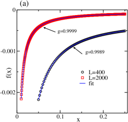
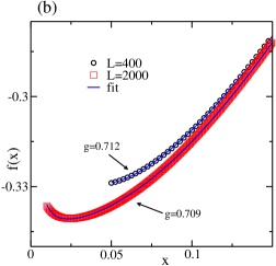
Figure 1: The function $f(x)$ vs. $x$ for the transverse field Ising chain and two system sizes (see legends). The symbols are the numerical data and the continuous lines are the best fit to Eq. (5). The arrows indicate the values of $g$ we get by the fitting procedure. (a) Results for the OBC case with zero boundary magnetic fields. (b) Results for the boundary magnetic field case with $\theta=\pi/4$, $\phi=\pi/4$ and $b=4$.

Now, we discuss the case of arbitrary direction of the boundary magnetic fields. As mentioned before, we are going to consider that the boundary magnetic fields are the same in both edges, i. e., $b_{1}=b_{L}=b$, $\theta_{1}=\theta_{L}=\theta$ and $\phi_{1}=\phi_{L}=\phi$. Then, the magnitude of the effective boundary magnetic fields in the directions $x$, $y$ and $z$ are $h_{x}^{b}=b\sin\theta\cos\phi$, $h_{y}^{b}=b\sin\theta\sin\phi$, and $h_{z}^{b}=b\cos\theta$, respectively for both edges. For systems with boundaries we must be careful when we use the Eq. (5) to get estimates of $g$, since Eq. (2) holds only if the crossover lengths $\xi\sim h_{b}^{d-1}<\ell$. The scaling dimension of the relevant boundary perturbation (in the $x$ direction) for the transverse field Ising chain is $d_{x}=1/2$ Cardy (1989); Cardy and Lewellen (1991). For instance, we need to be careful when we estimate $g$ for $\theta\rightarrow 0$ and/or $\phi\rightarrow\pi/2$, since the crossover length $\xi^{x}\thicksim(b\sin\theta\cos\phi)^{-1/2}$, for a finite boundary magnetic field, can diverge in these regimes. Due to this facts, we expect a huge crossover effect mainly if $\theta\rightarrow 0$ and/or $\phi\rightarrow\pi/2$ since $\xi^{x}\thicksim 1/\sqrt{b\theta\left(\pi/2-\phi\right)}$. In most of the cases, we observed that for the interval $1\leq b\leq 10$, the estimate of $g$ changes very little, which is indicative that we are in the regime that $\xi<\ell$.

It is also important to mention that for $\phi=\pi/2$ and $\theta\in$$(0,\pi/2]$ the matrix $M$ has four zero eigenvalues, while for $\theta=0$ and $\phi\in$$[0,\pi/2]$ has six zero eigenvalues. In these two regimes, the correlation matrix approach, presented before, to obtain the entanglement entropy needs a bit of modification, because if one does not take into account the extra degeneracies the matrix $U$ will not necessarily be in the desired canonical form, see Eq. (17). We will analyze those situations later. For other values of $\theta$ and $\phi$ we found that the matrix $M$ has just two zero eigenvalues, whose eigenstates are given in the Eq. (22).

In Figs. 1(b), we present a representative result of the function $f(x)$ for the ADBFM case. For this particular example, where $\phi=\pi/4$, $\theta=\pi/4$ and $b=4$, we get $g\sim 0.709$ for $L=2000$, which is very close to the expected exact value $g_{fixed}^{Ising}=\sqrt{2}/2=0.7071...$ Cardy (1989); Cardy and Lewellen (1991); Barthel et al. (2006). Using the explained fitting procedure, we estimated $g(\theta,\phi)$ for several other values of angles for system sizes $L=2000$. The obtained values are depicted in Fig. 2. As we can see in this figure, for $\phi\neq\pi/2$ and $\theta\notin$$(0,\pi/2]$ as well as for $\theta\neq 0$ and $\phi\notin$$[0,\pi/2]$ the results strongly indicate that $g(\theta,\phi)=\sqrt{2}/2$, except for small values of $\theta$ and $\phi$ close to $\pi/2$. As we already mentioned, in this region we expected a huge crossover effect for a finite boundary magnetic field. For instance, for $\theta=0.1\pi$ and $\phi=0.45\pi$, and considering $b=500$ we got $g=0.94$ and $g=0.83$ for $L=400$ and $L=2000$, respectively. We also observed that for a fixed value of $L$ the estimate of $g$ depends on the value of $b$. These finite-size effects are indicative that even for $b=500$, and $L=2000$ we are still not in the regime that $\xi^{x}<\ell$ for this angles.

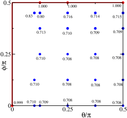
Figure 2: The numerical estimates of the ground state degeneracy $g(\theta,\phi)$ of the transverse field Ising chain for $L=2000$ and $b=4$. For $\phi=0.45$ and $\theta=0.1\pi$ and $\theta=0.125\pi$ exceptionally we used $b=500$. The circles are the points $(\theta,\phi)$ that we consider and the values close to them are the estimates of $g$ we get by the fitting procedure (see text). The results indicate that along the red lines we have $g=1$ and away from these lines we have $g=\sqrt{2}/2=0.707.$

Now, we consider the case $\theta=0$, where we have $b_{i}\cdot\vec{S}_{i}=\frac{b_{1}}{2}\sigma_{i}^{z}=b_{i}\left(c_{i}^{\dagger}c_{j}-1/2\right)$, $i=1$ and $L$. In this case, $b_{i}\cdot\vec{S}_{i}$ is quadratic in terms of creation and annihilations operators, so it is possible to map $H^{XY}$ to a quadratic free fermion Hamiltonian, and we can use the standard matrix correlation method to obtain the entanglement entropy. Since this perturbation is not relevant, we expect that the BE in this case be the same as the OBC case, i. e., $s_{b}=0$ (or equivalently $g=1).$ Indeed, our numerical estimates of $g$, based on the fitting procedure, agree very well with the expected value. For $b=4$ we get $g=0.998$ and $g=0.999$ for $L=400$ and $L=2000,$ respectively.

Finally, we discuss the case $\phi=\pi/2$. As we mentioned before, in this case we have four zero eigenvalues. Two eigenvectors, associated with these eigenvalues, are those given in Eq. (22) and the other two are

$$\ |u_{0}^{1}\rangle=\frac{1}{N_{nor}}\begin{pmatrix}\alpha i\\ 2\\ 0\\ \vdots\\ 0\\ -2\\ -\alpha i\\ -\alpha i\\ 2\\ 0\\ \vdots\\ 0\\ 2\\ -\alpha i\end{pmatrix},\hskip 14.22636pt|u_{0}^{2}\rangle=\frac{1}{N_{nor}}\begin{pmatrix}\alpha i\\ 2\\ 0\\ \vdots\\ 0\\ 2\\ \alpha i\\ -\alpha i\\ 2\\ 0\\ \vdots\\ 0\\ -2\\ \alpha i\end{pmatrix},$$ (78)

where $\alpha=2b\left(\cot\theta-\sec\theta\right)$ and $N_{nor}=2\sqrt{2\alpha^{2}+4}.$ The boundary perturbation now is given by $b_{i}\cdot\vec{S}_{i}=\frac{b_{1}}{2}\left(\sin\theta\sigma_{i}^{y}+\cos\theta\sigma_{i}^{z}\right),$ $i=1$ and $L$, and is not relevant too. Due to this fact, here too we expect that $g=1$ along the line with $\phi=\pi/2$. Again, our numerical data supports this prediction. We found that $g\sim 1.000$ along this line.

In summary as far as the boundary magnetic field vector is in the $yz$ plane one gets free boundary condition. Introducing even a small boundary magnetic field in the $x$ direction which means breaking the bulk $Z_{2}$ symmetry induces a fixed boundary condition.

IV The XXZ chain with arbitrary direction of the boundary magnetic field

In this section, we investigate the spin-1/2 $XXZ$ chain with ADBMF given by

$$\ \textbf{H}^{XXZ}=J\sum_{j=1}^{L-1}\Big{[}S_{j}^{x}S_{j+1}^{x}+S_{j}^{y}S_{j+1}^{y}+\Delta S_{j}^{z}S_{j+1}^{z}\Big{]}$$

$$+\vec{b}_{1}\cdot\vec{S}_{1}+\vec{b}_{L}\cdot\vec{S}_{L}\,,\hskip 51.21504pt$$ (79)

where $\Delta$ is the anisotropy and we use $J=1$ in order to fix the energy scale. The boundary magnetic fields $\vec{b}_{i}$, $i=1$ and $L$, are defined in Eqs. (7) and (8) and we consider that the magnitude of both boundary magnetic fields are the same, i. e. $b=b_{1}=b_{L}$. For $-1<\Delta\leq 1$ the system is bulk critical with central charge $c=1$. The OBC case corresponds to the free conformally invariant boundary condition with $g=g^{OBC}=\frac{1}{\pi^{1/4}\sqrt{2R}}$, where $R^{2}=\frac{1}{2\pi}\left(1-\frac{\arccos\Delta}{\pi}\right)$ Affleck (1998). While the fixed conformally invariant boundary condition with $g=g^{fixed}=\pi^{1/4}\sqrt{R}$ corresponds to the case that both boundary magnetic fields are in the $x$ direction ($\phi_{1}=\phi_{2}=0$ and $\theta=\frac{\pi}{2}$) with $b_{1}=b_{L}=\infty$ Affleck (1998). Note that these predictions were obtained by bosonization technique and to our knowledge they were not verified by other entanglement approaches. It is important to mention that although the XXZ chain with ADBMF is exactly solvable by the thermodynamic Bethe ansatz methodde Vega and Ruiz (1993); Nepomechie (2002, 2003); Cao et al. (2003, 2013a, 2013b); Niccoli (2013); Faldella et al. (2014); Belliard (2013); Kitanine et al. (2014); Nepomechie and Wang (2013); Li et al. (2014); Pozsgay and Rákos (2018), it seems in the massless regime the determination of the free boundary energy in the low temperature regime is not simple. Thus, it is highly desirable to confirm the bosonization prediction by other unbiased techniques. Furthermore, there is no prediction of the values of $g$ for other directions of the boundary magnetic fields. We intent to provide further insight about these issues, in this section. It is also important to mention that, like the Ising case when the edge magnetic fields are the same and are in the $x$ direction, here too if we choose $J<0$ the corrections in $S^{b}(L,\ell)$ are zero, i. e. $G_{b}=0$. However, for positive values of $J$ those corrections are present.

Before starting to present the results, it is convenient to mention that in the case that both boundary magnetic fields are the same, we verified, numerically, that the energies as well as the entanglement entropy of the XXZ chain do not depend on the values of the angle $\phi=\phi_{1}=\phi_{L}$. Another important point is that in the case of the XX chain with ADBMF [$\Delta=0$ in Eq. (79)], the Hamiltonian is the same as the one in Eq. (6) with $\gamma=0$ and $h=0$. Consequently, we can use the correlation matrix method developed in the previous section to obtain the entanglement entropy.

We first consider the XX chain with OBC. In Fig. 3(a), we show the function $f(x)$ defined in Eq. (5) for the XX chain with OBC. By fitting the numerical data to this equation we get $g=1.0002$ and $g=1.0001$ for $L=600$ and $L=2000$, respectively. Similar agreement with the bosonization prediction is found also for the XXZ under OBC, as depicted in Table 1 for two other values of $\Delta$. For $\Delta=0.5$ and $\Delta=\cos{(\pi/8)=0.9238...\,}$, we used the DMRG to obtain the entanglement entropy. For the systems under PBC (OBC and ADBMF) we kept up to $m=3000$ ($m=800$) states per block in the final sweep and done $\sim 6-8$ sweeps. The discarded weight was typically around $10^{-10}-10^{-12}$ at that final sweep.

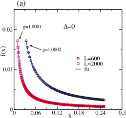
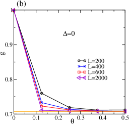
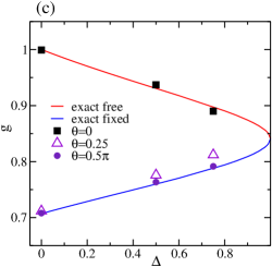
Figure 3: (a) The function $f(x)$ vs. $x$ for XX chain and two system sizes (see legends). The symbols are the numerical data and the continuous lines are the best fit to Eq. (5). The arrows indicate the values of $g$ we get by the fitting procedure. (b) Estimates of $g$ for the XX chain with $b_{1}=b_{L}=1$ and for some values of $\theta$ and $L$. The orange solid line correspond to $g=\sqrt{2}/2\equiv g^{fixed}$. (c) Values of $g$ for the XXZ chain for some boundary conditions (see text). The solid lines are the bosonization predictions while the symbols are numerical estimates obtained considering systems with sizes $L=600$.

$\Delta$
	$0$	$0.5$	$0.9238$
$g^{OBC}$	1.0002	0.9309	0.8784
	(1.0000)	(0.9306)	(0.8694)

Table 1: The estimates of ground state degeneracy, $g^{OBC}$, for XXZ Heisenberg chain with OBC and $L=600$ for three values of anisotropy parameter $\Delta$. The results in parentheses are the predicted ones (see text).

Finally we consider the $XXZ$ chain with ADBMF. Here too, we first focus on the XX chain. In Fig. 3(b), we preset some values of $g$ obtained by the fitting procedure for the XX chain with some values of $\theta$. Note that For $L=600$ and $\theta=0.5\pi$, which corresponds to the magnetic field in the $x$ direction we get $g=0.708$. In this situation, it is expected that the system corresponds to a fixed conformally invariant boundary condition with $g^{fixed}=\sqrt{2}/2$ Affleck (1998). Indeed, our result agrees very well with the bosonization prediction for the $x$ direction. For the other directions of the boundary magnetic fields, which to our knowledge were not considered so far in the literature, our estimates also indicate that for $0<\theta\leq\pi/2$ we have $g=g^{fixed}=\sqrt{2}/2$, as one can observe in Fig. 3(b). The crossover length $\xi^{x}\sim h_{b}^{d-1}$ associated with the boundary perturbations of the boundary magnetic fields $x$ and $z$ directions have dimensions $d_{x}=2\pi R^{2}$ and $d_{z}=1$, respectively Affleck (1998). Since the boundary perturbation in the $z$ direction is marginal logarithmic corrections may appear. Note that for $\theta\sim 0$ we have $\xi^{x}\sim(b\theta)^{2\pi R^{2}-1}$ and similar to the transverse field Ising case a huge crossover length is expected close to $\theta=0$ for finite boundary magnetic fields. We also estimate $g$ for other two values of the $\Delta$ [see Fig. 3(c)] and different directions of magnetic fields. We summarize in Fig. 3(c) all the estimates of $g$ that we obtained for the XXZ chain for different boundary conditions for system sizes $L=600$ and $b=1$. As we can observe in this figure, our results strongly support that $g=g^{fixed}=\pi^{1/4}\sqrt{R}$ for $0<\theta\leq\pi/2$ and $g=g^{OBC}=\frac{1}{\pi^{1/4}\sqrt{2R}}$ for $\theta=0$.

In summary as far as the boundary magnetic field vector is in the $z$ direction, i.e. $\theta=0$ one gets free boundary condition. Introducing even a small boundary magnetic field in the $x$ and/or $y$ direction which breaks the bulk $U(1)$ symmetry induces a fixed boundary condition.

V Conclusions

In this paper, we investigated entanglement entropy in open quantum critical spin chains with arbitrary boundary magnetic fields. The evaluating of the boundary entropy in such systems, in general, is not a simple task by using the thermodynamic Bethe ansataz method or the CFT approach. Here, we present a simple procedure to estimate the boundary entropy by considering the finite-size corrections of the entanglement entropies and without the knowledge of the non-universal correction $G_{b}$ which is induced by the boundaries Taddia et al. (2013), see Eqs. (2)-(5). In particular, we calculated the boundary entropy in the critical transverse field Ising chain and the critical XXZ chain. We were able to obtain precise estimates of the universal boundary entropy of these two models that were in perfect agreement with previous analytical predictions. In particular, we provided estimates of the universal boundary entropy for directions of the boundary magnetic field that were not investigated in the literature so far. Our results support that if the boundary magnetic field breaks the bulk symmetry then we have a fixed boundary condition and if it does not we have a free boundary condition. One of our technical achievements was the exact solution of the XY chain with ADBMF which to the best of our knowledge has not been tackled so far. Our exact solution gives all the spectrum and the eigenstates of the Hamiltonian. Using this solution we were able to calculate the entanglement entropy using the modified version of the correlation method up to relatively large subsystem sizes, $L=2000$. To do similar calculations for the XXZ chain we used the DMRG.

Acknowledgements. We thank B Pozsgay for bringing in our attention to the reference [Pozsgay and Rákos, 2018]. MAR thanks A. Jafarizadeh for discussions. MAR acknowledges partial support from CNPq and FAPERG (grant number 210.354/2018). JCX acknowledges the support from CAPES and FAPEMIG.

Appendix A Calculation of $\delta_{+}$

In this Appendix, we show how to calculate $\delta_{+}=\langle\tilde{G}_{+}|\sigma^{x}_{L+1}|\tilde{G}_{+}\rangle$. First of all it is easy to see that

$$\ \delta_{+}=\langle\tilde{G}_{+}|\sigma^{x}_{L+1}|\tilde{G}_{+}\rangle=\hskip 113.81102pt$$

$$(-i)^{L+1}\langle\tilde{G}_{+}|a_{0}^{y}\prod_{k=1}^{L}a_{k}^{x}a_{k}^{y}a_{L+1}^{x}|\tilde{G}_{+}\rangle.\hskip 14.22636pt$$ (80)

Since just $a_{0}^{x}$ and $a_{L+1}^{y}$ depend on the $\eta_{0}$ and $\eta_{0}^{\dagger}$ one can write

$$\ \delta_{+}=(-i)^{L+1}\langle\tilde{0}|a_{0}^{y}\prod_{k=1}^{L}a_{k}^{x}a_{k}^{y}a_{L+1}^{x}|\tilde{0}\rangle.$$ (81)

Because of the Wick’s theorem one can write the above correlation as a Pfaffian as follows

$$\ \delta_{+}=(-i)^{L+1}\text{Pf}[\textbf{D}],$$ (82)

where

$$\ \textbf{D}=\begin{pmatrix}0&\langle a_{0}^{y}a_{1}^{x}\rangle&\langle a_{0}^{y}a_{1}^{y}\rangle&...&\langle a_{0}^{y}a_{L+1}^{x}\rangle\\ \langle a_{1}^{x}a_{0}^{y}\rangle&0&\langle a_{1}^{x}a_{1}^{y}\rangle&...&\langle a_{1}^{x}a_{L+1}^{x}\rangle\\ \langle a_{1}^{y}a_{0}^{y}\rangle&\langle a_{1}^{y}a_{1}^{x}\rangle&0&...&\langle a_{1}^{y}a_{L+1}^{x}\rangle\\ .&.&.&.&.\\ .&.&.&.&.\\ .&.&.&.&.\\ \langle a_{L+1}^{x}a_{0}^{y}\rangle&\langle a_{L+1}^{x}a_{1}^{x}\rangle&\langle a_{L+1}^{x}a_{1}^{y}\rangle&...&0\end{pmatrix}.$$ (83)

Appendix B The $\ln{2}$ term in the EE

For the cases that the reduced density matrix is build using an state that one site is not entanglement with the others sites, we need to be careful when we use the correlation matrix method to calculate $S(L,\ell)$. In this Appendix, we show why we should subtract the $\ln 2$ in the entanglement entropy for a particular situation.

For simplicity, let us consider the following free fermion Hamiltonian

$$H=\sum_{i,j}^{L}c_{i}^{\dagger}H_{i,j}c_{j}\;.$$ (84)

Suppose that we project the ground state of the above Hamiltonian to obtain the state $\mid\Psi_{0}^{L}\rangle=\mid+\rangle\otimes\mid\Psi_{0}^{L-1}\rangle$, where $\mid+\rangle=\frac{1}{\sqrt{2}}\left(\mid 1\rangle+\mid 0\rangle\right)$ and $c_{1}^{\dagger}c_{1}\mid n\rangle=n\mid n\rangle$, $n=0,1$.

Let us focus in the following density matrix

$$\rho=\mid\Psi_{0}^{L}\rangle\langle\Psi_{0}^{L}\mid=\mid+\rangle\langle+\mid\otimes\mid\Psi_{0}^{L-1}\rangle\langle\Psi_{0}^{L-1}\mid\;.$$ (85)

So, the reduced density matrix is given by

$$\rho_{A}={\rm tr}_{B}\;\rho\;=(\frac{1+c_{1}^{\dagger}+c_{1}}{2})\tilde{\rho}_{A}\;,$$ (86)

where we have defined the reduced density matrix associated with the sites $2,...,\ell$ as

$$\tilde{\rho}_{A}={\rm tr}_{B}\mid\Psi_{0}^{L-1}\rangle\langle\Psi_{0}^{L-1}\mid=\frac{e^{-h_{A}}}{{\rm tr}\;e^{-h_{A}}}\;.$$ (87)

We are going to assume that $\tilde{\rho}_{A}$ can be written in a diagonal form in terms of new creation/annihilation operator as

$$\tilde{\rho}_{A}=\frac{e^{{-\sum_{k=2}^{\ell}\epsilon_{k}d_{k}^{\dagger}d_{k}}}}{{\rm tr}\;e^{-h_{A}}}\;.$$ (88)

Due to this fact, the eigenvalues $\epsilon_{k}$ are associated with the eigenvalues $\lambda_{k}$ of the correlation matrix $C_{i,j}={\rm tr}_{A}\left(\rho_{A}c_{i}^{\dagger}c_{j}\right)$, with $i,j=2,...,\ell$ by $\lambda_{k}=(1+e^{\epsilon_{k}})^{-1}\equiv\frac{1-\nu_{k}}{2}$ Peschel (2003). And the entanglement entropy for that kind of state is given by Peschel (2003)

$$S(L,\ell)=-\sum_{k=2}^{\ell}[\frac{1+\nu_{k}}{2}\ln\frac{1+\nu_{k}}{2}+\frac{1-\nu_{k}}{2}\ln\frac{1-\nu_{k}}{2}]\;,\ell=2,...L\,,$$ (89)

and for $\ell=1$ we have that S(L,1)=0.

Now, suppose that instead of considering the correlation matrix $C_{i,j}$ we define the following correlation matrix $\tilde{C}_{i,j}={\rm tr}_{A}\left(\rho_{A}c_{i}^{\dagger}c_{j}\right)$, with $i,j=1,2,...,\ell$. It is simple to show that $\tilde{C}_{1,j}=1/2\;\delta_{1,j}$. Due to this fact, the eigenvalues of the matrix $\tilde{C}$ are the same eigenvalues as $C$ plus the eigenvalue $\lambda_{1}=1/2$ (which correspond to $\nu_{1}=0$). So, we see that if we associate the entanglement entropy $\tilde{S}$ with the eigenvalues of the correlation matrix $\tilde{C}$, we realize that $\tilde{S}(L,\ell)=\ln 2+S(L,\ell)$.

References

- Laflorencie (2016) N. Laflorencie, Physics Reports 646, 1 (2016).
- Casini and Huerta (2009) H. Casini and M. Huerta, J. Phys. A: Math. Theor. 42, 504007 (2009).
- Castro-Alvaredo and Doyon (2009a) O. A. Castro-Alvaredo and B. Doyon, J. Phys. A: Math. Theor. 42, 504006 (2009a).
- Calabrese and Cardy (2009) P. Calabrese and J. Cardy, J. Phys. A: Math. Theor. 42, 504005 (2009).
- Laflorencie et al. (2006) N. Laflorencie, E. S. Sørensen, M.-S. Chang, and I. Affleck, Phys. Rev. Lett. 96, 100603 (2006).
- Zhou et al. (2006) H.-Q. Zhou, T. Barthel, J. O. Fjærestad, and U. Schollwöck, Phys. Rev. A 74, 050305 (2006).
- Legeza et al. (2007) O. Legeza, J. Sólyom, L. Tincani, and R. M. Noack, Phys. Rev. Lett. 99, 087203 (2007).
- Szirmai et al. (2008) E. Szirmai, O. Legeza, and J. Sólyom, Phys. Rev. B 77, 045106 (2008).
- Castro-Alvaredo and Doyon (2009b) O. A. Castro-Alvaredo and B. Doyon, Journal of Statistical Physics 134, 105–145 (2009b).
- Affleck et al. (2009) I. Affleck, N. Laflorencie, and E. S. Sørensen, J. Phys. A: Math. Theor. 42, 504009 (2009).
- Taddia et al. (2013) L. Taddia, J. C. Xavier, F. C. Alcaraz, and G. Sierra, Phys. Rev. B 88, 075112 (2013).
- Fagotti and Calabrese (2011) M. Fagotti and P. Calabrese, J. Stat. Mech. 2011, P01017 (2011).
- Diehl (1997) H. W. Diehl, Int. J. Mod. Phys. B 11, 3503–3523 (1997).
- Affleck and Ludwig (1991) I. Affleck and A. W. W. Ludwig, Phys. Rev. Lett. 67, 161 (1991).
- Calabrese and Cardy (2004) P. Calabrese and J. Cardy, J. Stat. Mech. 2004, P06002 (2004).
- Najafi and Rajabpour (2016) K. Najafi and M. A. Rajabpour, Journal of High Energy Physics 2016, 124 (2016).
- Alba et al. (2017) V. Alba, P. Calabrese, and E. Tonni, J. Phys. A: Math. Theor. 51, 024001 (2017).
- Tu (2017) H.-H. Tu, Phys. Rev. Lett. 119, 261603 (2017).
- Tang et al. (2017) W. Tang, L. Chen, W. Li, X. C. Xie, H.-H. Tu, and L. Wang, Phys. Rev. B 96, 115136 (2017).
- Barthel et al. (2006) T. Barthel, M.-C. Chung, and U. Schollwöck, Phys. Rev. A 74, 022329 (2006).
- Bilstein and Wehefritz (1999) U. Bilstein and B. Wehefritz, J. Phys. A: Math. Theor. 32, 191 (1999).
- Peschel (2003) I. Peschel, J. Phys. A: Math. Theor. 36, L205 (2003).
- White (1992) S. R. White, Phys. Rev. Lett. 69, 2863 (1992).
- Schollwöck (2005) U. Schollwöck, Rev. Mod. Phys. 77, 259 (2005).
- Cardy (1989) J. L. Cardy, Nuclear Physics B 324, 581 (1989).
- Cardy and Lewellen (1991) J. L. Cardy and D. C. Lewellen, Physics Letters B 259, 274 (1991).
- Friedan and Konechny (2004) D. Friedan and A. Konechny, Phys. Rev. Lett. 93, 030402 (2004).
- Holzhey et al. (1994) C. Holzhey, F. Larsen, and F. Wilczek, Nuclear Physics B 424, 443 (1994).
- Vidal et al. (2003) G. Vidal, J. I. Latorre, E. Rico, and A. Kitaev, Phys. Rev. Lett. 90, 227902 (2003).
- Korepin (2004) V. E. Korepin, Phys. Rev. Lett. 92, 096402 (2004).
- Alcaraz et al. (2011) F. C. Alcaraz, M. I. Berganza, and G. Sierra, Phys. Rev. Lett. 106, 201601 (2011).
- Essler et al. (2013) F. H. L. Essler, A. M. Läuchli, and P. Calabrese, Phys. Rev. Lett. 110, 115701 (2013).
- Calabrese et al. (2010) P. Calabrese, M. Campostrini, F. Essler, and B. Nienhuis, Phys. Rev. Lett. 104, 095701 (2010).
- Cardy and Calabrese (2010) J. Cardy and P. Calabrese, J. Stat. Mech. 2010, P04023 (2010).
- Xavier and Alcaraz (2012) J. C. Xavier and F. C. Alcaraz, Phys. Rev. B 85, 024418 (2012).
- Ercolessi et al. (2012) E. Ercolessi, S. Evangelisti, F. Franchini, and F. Ravanini, Phys. Rev. B 85, 115428 (2012).
- Dalmonte et al. (2011) M. Dalmonte, E. Ercolessi, and L. Taddia, Phys. Rev. B 84, 085110 (2011).
- Affleck (1998) I. Affleck, J. Phys. A: Math. Theor. 31, 2761 (1998).
- Colpa (1979) J. H. P. Colpa, J. Phys. A: Math. Theor. 12, 469 (1979).
- Bariev and Peschel (1991) R. Bariev and I. Peschel, Physics Letters A 153, 166 (1991).
- Campostrini et al. (2015) M. Campostrini, A. Pelissetto, and E. Vicari, J. Stat. Mech. 2015, P11015 (2015).
- Chung and Peschel (2001) M.-C. Chung and I. Peschel, Phys. Rev. B 64, 064412 (2001).
- Jin and Korepin (2004) B.-Q. Jin and V. E. Korepin, Journal of Statistical Physics 116, 79 (2004).
- de Vega and Ruiz (1993) H. J. de Vega and A. G. Ruiz, J. Phys. A: Math. Theor. 26, L519 (1993).
- Nepomechie (2002) R. I. Nepomechie, Nuclear Physics B 622, 615 (2002).
- Nepomechie (2003) R. I. Nepomechie, J. Phys. A: Math. Theor. 37, 433 (2003).
- Cao et al. (2003) J. Cao, H.-Q. Lin, K.-J. Shi, and Y. Wang, Nuclear Physics B 663, 487 (2003).
- Cao et al. (2013a) J. Cao, W.-L. Yang, K. Shi, and Y. Wang, Nuclear Physics B 875, 152 (2013a).
- Cao et al. (2013b) J. Cao, W.-L. Yang, K. Shi, and Y. Wang, Nuclear Physics B 877, 152 (2013b).
- Niccoli (2013) G. Niccoli, Nuclear Physics B 870, 397 (2013).
- Faldella et al. (2014) S. Faldella, N. Kitanine, and G. Niccoli, J. Stat. Mech. 2014, P01011 (2014).
- Belliard (2013) S. Belliard, Symmetry, Integrability and Geometry: Methods and Applications (2013), 10.3842/sigma.2013.072.
- Kitanine et al. (2014) N. Kitanine, J. M. Maillet, and G. Niccoli, J. Stat. Mech. 2014, P05015 (2014).
- Nepomechie and Wang (2013) R. I. Nepomechie and C. Wang, J. Phys. A: Math. Theor. 47, 032001 (2013).
- Li et al. (2014) Y.-Y. Li, J. Cao, W.-L. Yang, K. Shi, and Y. Wang, Nuclear Physics B 884, 17 (2014).
- Pozsgay and Rákos (2018) B. Pozsgay and O. Rákos, J. Stat. Mech. 2018, 113102 (2018).
- Note (1) We thanks B. Pozsgay for pointing this fact to us.