Stability of Kerr black holes in generalized hybrid metric-Palatini gravity

Abstract

It is shown that the Kerr solution exists in the generalized hybrid metric-Palatini gravity theory and that for certain choices of the function $f(R,\mathcal{R})$ that characterizes the theory, the Kerr solution can be stable against perturbations on the scalar degree of freedom of the theory. We start by verifying which are the most general conditions on the function $f(R,\mathcal{R})$ that allow for the general relativistic Kerr solution to also be a solution of this theory. We perform a scalar perturbation in the trace of the metric tensor, which in turn imposes a perturbation in both the Ricci and Palatini scalar curvatures. To first order in the perturbation, the equations of motion, namely the field equations and the equation that relates the Ricci and the Palatini curvature scalars, can be rewritten in terms of a fourth-order wave equation for the perturbation $\delta R$ which can be factorized into two second-order massive wave equations for the same variable. The usual ansatz and separation methods are applied and stability bounds on the effective mass of the Ricci scalar perturbation are obtained. These stability regimes are studied case by case and specific forms of the function $f(R,\mathcal{R})$ that allow for a stable Kerr solution to exist within the perturbation regime studied are obtained.

I Introduction

General relativity, a relativistic theory of gravitation, see e.g. mtw , has passed a great number of tests, from the weak-field tests within the Solar System to strong-field tests that include black holes and gravitational waves. In a cosmological setting, one needs to add to the ingredients of general relativity some form of dark matter to deal with the large-scale structure of the Universe, and to postulate a cosmological constant, or a variant of it, to explain the acceleration of the Universe.

In alternative to general relativity plus dark matter and cosmological constant package, one can use a modified theory of gravitation, an extension of general relativity, by modifying the gravitational sector of the theory. In this way one can also address the structure and dynamics of the known self-gravitating systems and account for the Universe’s self-accelerated cosmic expansion. In $f(R)$ gravity modgrav ; modgrav2 ; modgrav3 ; Capozziello:2011et , it has been established that both metric and Palatini Olmo:2011uz versions of these theories have interesting features but also manifest severe and different downsides. To overcome these problems, a hybrid combination of theories, containing elements from both formalisms, turns out to be fruitful in accounting for the observed phenomenology and in addition is able to avoid some drawbacks of the original approaches. This approach is known as the hybrid metric-Palatini gravity harko ; capozziello . The action that describes this theory is obtained from the usual Einstein-Hilbert action $R$ by the addition of a function $f(\mathcal{R})$, where $\mathcal{R}$ is a curvature scalar defined in terms of an independent connection $\hat{\Gamma}$. In this theory, the metric and the affine connection are considered to be independent degrees of freedom, therefore combining both the metric and the Palatini formalisms into a new modified gravity. This theory was shown to be very successful in accounting for observed phenomena in cosmological capozziello2 and galactic dynamics capozziello3 ; Capozziello:2012qt , leaving the Solar System constraints unaffected harko . For a comprehensive and extensive review on the hybrid metric-Palatini theory see BookHarkoLobo .

The generalized hybrid metric-Palatini (GHMP) gravity arises as a natural outcome of the hybrid metric-Palatini gravity, where the action $R+f(\mathcal{R})$ is replaced by a general function $f(R,\mathcal{R})$ of both the Ricci and Palatini scalar curvatures tamanini . This theory was studied in the context of cosmology, both with dynamical systems methods tamanini and with reconstruction techniques rosa1 , for which it was shown, among other behaviors, that exponentially expanding cosmological models exist even when the matter distribution is not purely vacuum. Also, asymptotically anti-de Sitter wormhole solutions with thin shells that satisfy the null energy condition for the whole spacetime were obtained in this theory rosa2 .

General relativity has produced as solutions, the static, i.e., Schwarzschild, black hole, and the rotating, i.e. Kerr Kerr:1963ud , black hole, which mirror the observed rotating astrophysical black holes. As physically realistic objects, Kerr black holes must be stable against exterior perturbations. Within general relativity, the stability of Kerr black holes has been studied for scalar, vectorial and tensorial perturbations. For massless perturbations, the Kerr black hole was shown to be stable teukolsky1974 ; chandrabook . For massive perturbations the issue is more subtle, see e.g. beyer . Moreover, for massive scalar, vectorial and tensor perturbations, the confinement of superradiant modes can lead to an amplification of the perturbation ad infinitum, giving rise to instabilities such as the black hole bomb press ; lemos1 .

In $f(R)$ gravity black hole solutions and perturbations have also been analyzed. An initial effort has been to reproduce and study within $f(R)$ gravity the Schwarzschild and Kerr solutions of general relativity. This theory was motivated to understand the acceleration of the Universe in a natural way, and thus in principle, it contains in it some form of a cosmological constant, meaning that the spacetime is asymptotically de Sitter. However, the Schwarzschild and Kerr solutions are asymptotically flat rather than asymptotically de Sitter, the rationale for using those, is that, as a first approximation, locally, the influence of the cosmological constant term is negligible and thus consideration of the Schwarzschild or Kerr solutions is justified, besides being more simple. Thus, confining to Schwarzschild or Kerr, perturbation analyses of those solutions have been performed within $f(R)$ gravity. For instance, the stability of the $f(R)$ Schwarzschild black hole in $f(R)$ theory was investigated in its scalar-tensor representation by introducing two auxiliary scalars myung1 . It was shown that the curvature scalar becomes a scalaron, so that the linearized equations are second order and in addition are the same equations as for the massive Brans-Dicke theory. Furthermore, it was proved that the $f(R)$ black hole solution is stable against external perturbations if the scalaron does not have a tachyonic mass. The analysis was even extended to include the stability of the Schwarzschild-AdS black hole in $f(R)$ theories with a negative cosmological constant Moon:2011sz with the conclusion that stable solutions against external perturbations exist if the scalaron is again free from tachyons. The stability of the Schwarzschild black hole was also analyzed in several extensions of $f(R)$ gravity Moon:2011fw ; Myung:2013doa ; Myung:2017qtc . The study of the stability of the Kerr solution in $f(R)$ gravity has been studied in Myung:2011we ; myung2 , where it has been proved that it is unstable due to the fact that the perturbation equation for the massive spin-0 graviton in this theory, or equivalently the perturbed Ricci scalar, is analogous to a Klein-Gordon equation for a massive scalar field in general relativity which has been intensively studied and showed to be unstable.

In GHMP gravity it is also important to analyze black holes and their stability. Again, the Schwarzschild and Kerr solutions are useful in this theory. The logic to study these solutions in $f(R,\mathcal{R})$ gravity is the same as that used in $f(R)$, namely, although GHMP gravity was motivated to understand the acceleration of the Universe having some form of a cosmological constant, locally one can argue that the influence of it is negligible and thus the use of the Schwarzschild and Kerr solutions, rather than the asymptotically de Sitter counterparts, is justified. Since Kerr black holes are stable within general relativity it is of interest to know whether those black holes exist or not as solutions of the GHMP gravity and, in the case that the answer is positive, it is important to perform a stability analysis of the black holes themselves with the theory. A first step in that direction is to understand the perturbations in both the Ricci and Palatini scalar curvatures of $f(R,\mathcal{R})$ gravity within this setting and to work out for which choices of the function $f(R,\mathcal{R})$ Kerr black holes are stable to those perturbations. This is what we set out to do here.

The paper is organized as follows. In Sec. II, we introduce the action of the GHMP gravity and compute the respective equations of motion. In Sec. III, we start with a general form of the function $f$ that guarantees that constant Ricci scalar $R$ solutions exist in the GHMP gravity, and then choose the specific case of the Kerr metric to compute perturbations to the massive spin-0 degree of freedom. In Sec. IV, we compute the stability regimes of the perturbations and the forms of the function $f$ that allow for these regimes to be attained. In Sec. V, we conclude.

II Action and field equations of the GHMP gravity

Consider the action $S$ of the GHMP gravity given by

$$S=\frac{1}{2\kappa^{2}}\int_{\Omega}\sqrt{-g}f(R,{\cal R})d^{4}x+S_{m},$$ (1)

where $\kappa\equiv 8\pi G$, $G$ is the gravitational constant, $\Omega$ is the spacetime volume and $d^{4}x$ its volume element, $g$ is the determinant of the spacetime metric $g_{ab}$, $R$ is the metric Ricci scalar, $\mathcal{R}\equiv\mathcal{R}^{ab}g_{ab}$ is the Palatini Ricci scalar, where the Palatini Ricci tensor is defined in terms of an independent connection $\hat{\Gamma}^{c}_{ab}$ as,

$$\mathcal{R}_{ab}=\partial_{c}\hat{\Gamma}^{c}_{ab}-\partial_{b}\hat{\Gamma}^{c}_{ac}+\hat{\Gamma}^{c}_{cd}\hat{\Gamma}^{d}_{ab}-\hat{\Gamma}^{c}_{ad}\hat{\Gamma}^{d}_{cb}\,,$$ (2)

$f(R,\cal{R})$ is a well-behaved function of $R$ and $\cal{R}$, and $S_{m}$ is the matter action defined as $S_{m}=\int d^{4}x\sqrt{-g}\;{\cal L}_{m}$, where ${\cal L}_{m}$ is the matter Lagrangian density considered minimally coupled to the metric $g_{ab}$. We set the speed of light to one, $c=1$. Equation (1) is the geometrical representation of the GHMP gravity. An equivalent scalar-tensor representation of the theory with two scalar fields is possible to obtain with the help of auxiliary scalar fields, see Appendix A.

Variation of the action (1) with respect to the metric $g_{ab}$ yields the following equation of motion,

$$\frac{\partial f}{\partial R}R_{ab}+\frac{\partial f}{\partial\mathcal{R}}\mathcal{R}_{ab}-\frac{1}{2}g_{ab}f(R,\cal{R})$$

$$-\left(\nabla_{a}\nabla_{b}-g_{ab}\Box\right)\frac{\partial f}{\partial R}=\kappa^{2}T_{ab},$$ (3)

where $\nabla_{a}$ is the covariant derivative and $\Box=\nabla^{a}\nabla_{a}$ is the d’Alembertian operator, both with respect to $g_{ab}$, and $T_{ab}$ is the stress-energy tensor defined in the usual manner as

$$T_{ab}=-\frac{2}{\sqrt{-g}}\frac{\delta(\sqrt{-g}\,{\cal L}_{m})}{\delta(g^{ab})}\,.$$ (4)

Varying the action (1) with respect to the independent connection $\hat{\Gamma}^{c}_{ab}$ provides the following relationship,

$$\hat{\nabla}_{c}\left(\sqrt{-g}\,\frac{\partial f}{\partial\cal{R}}g^{ab}\right)=0\,,$$ (5)

where $\hat{\nabla}_{a}$ is the covariant derivative with respect to the connection $\hat{\Gamma}^{c}_{ab}$. Now recalling that $\sqrt{-g}$ is a scalar density of weight 1, we have that $\hat{\nabla}_{c}\sqrt{-g}=0$ and so Eq. (5) simplifies to $\hat{\nabla}_{c}\left(\frac{\partial f}{\partial\cal{R}}g^{ab}\right)=0$. This means that there exists a new metric $h_{ab}$ defined as

$$h_{ab}=g_{ab}\frac{\partial f}{\partial\cal{R}}$$ (6)

such that the connection $\hat{\Gamma}^{a}_{bc}$ is the Levi-Civita connection for this metric, i.e.

$$\hat{\Gamma}^{a}_{bc}=\frac{1}{2}h^{ad}\left(\partial_{b}h_{dc}+\partial_{c}h_{bd}-\partial_{d}h_{bc}\right)\,,$$ (7)

where $\partial_{a}$ denotes a partial derivative. Note also from Eq. (6) that $h_{ab}$ is conformally related to $g_{ab}$ through the conformal factor ${\partial f}/{\partial\cal{R}}$. This result implies that the two Ricci tensors $R_{ab}$ and $\mathcal{R}_{ab}$, that we assumed to be independent at first, are actually related to each other by

$$\mathcal{R}_{ab}=R_{ab}-\frac{1}{f_{\mathcal{R}}}\left(\nabla_{a}\nabla_{b}+\frac{1}{2}g_{ab}\Box\right)f_{\mathcal{R}}+\frac{3}{2f_{\mathcal{R}}^{2}}\partial_{a}f_{\mathcal{R}}\partial_{b}f_{\mathcal{R}},$$ (8)

where the subscripts $R$ and $\mathcal{R}$ denote derivatives of the function $f$ with respect to either $R$ and $\mathcal{R}$, respectively. Note that we shall be working with forms of the function $f$ that satisfy the Schwartz theorem, which means that its crossed derivatives are the same, i.e., $f_{R\mathcal{R}}=f_{\mathcal{R}R}$. We therefore have a system of two independent equations of motion, Eqs. (II) and (8), the latter being equivalent to Eq. (5).

III Perturbations in GHMP of general relativity solutions with $R_{ab}=0$

III.1 General conditions on the function $f(R,\mathcal{R})$

In this section we assume a general form for the function $f(R,\mathcal{R})$ that guarantees that general relativity solutions with $R_{ab}=0$, such as the Schwarzschild and Kerr solutions, are also solutions of the GHMP theory.

To do so, let us assume two very general conditions for the function $f(R,\mathcal{R})$. First, consider that the function $f$ is analytical in both $R$ and $\mathcal{R}$ around a point $\left\{0,\mathcal{R}_{0}\right\}$, where $\mathcal{R}_{0}$ is a constant, and therefore can be expanded in a Taylor series of the form

$$f(R,\mathcal{R})=\sum_{\left\{n,m\right\}=0}^{\infty}\frac{\partial^{\left(n+m\right)}f\left(0,\mathcal{R}_{0}\right)}{\partial^{n}R\ \partial^{m}\mathcal{R}}\times$$

$$\times\frac{R^{n}}{n!}\frac{\left(\mathcal{R}-\mathcal{R}_{0}\right)^{m}}{m!}.$$ (9)

Second, impose that the function $f$ has a zero at the point where we perform the Taylor series expansion, that is

$$f\left(0,\mathcal{R}_{0}\right)=0.$$ (10)

We now show that for a function $f$ that satisfies these two conditions it is always possible for a general relativity solution with $R_{ab}=0$ and so $R=0$ to be also a solution in the GHMP gravity. To start with, let $X$ denote $R$, $\cal R$, or any combination of the form $R\cal R$, and so on, and let $f_{X}$ denote the derivative of $f$ with respect to $X$. Then, the derivatives of the functions $f_{X}$ with respect to the coordinates $x^{a}$ can be written as functions of the derivatives of $R$ and $\mathcal{R}$ by making use of the chain rule, from which we obtain

$$\partial_{a}f_{X}=f_{XR}\partial_{a}R+f_{X\mathcal{R}}\partial_{a}\mathcal{R},$$ (11)

which also allow us to write the terms $\nabla_{a}\nabla_{b}f_{X}$ and $\Box f_{X}$ as functions of $R$ and $\mathcal{R}$ as

$$\nabla_{a}\nabla_{b}f_{X}=f_{XRR}\nabla_{a}R\nabla_{b}R+f_{X\mathcal{R}\mathcal{R}}\nabla_{a}\mathcal{R}\nabla_{b}\mathcal{R}+$$

$$2f_{XR\mathcal{R}}\nabla_{(a}R\nabla_{b)}\mathcal{R}+f_{XR}\nabla_{a}\nabla_{b}R+f_{X\mathcal{R}}\nabla_{a}\nabla_{b}\mathcal{R},$$ (12)

where indices within parentheses are symmetrized, and

$$\Box f_{X}=g^{ab}\nabla_{a}\nabla_{b}f_{X}\,.$$ (13)

Now, let us first use Eq. (8) to eliminate the term $\mathcal{R}_{ab}$ in Eq. (II), from which we get $\left(f_{R}+f_{\mathcal{R}}\right)R_{ab}-\left(\nabla_{a}\nabla_{b}+\frac{1}{2}g_{ab}\Box\right)f_{\mathcal{R}}+\frac{3}{2f_{\mathcal{R}}}\partial_{a}f_{\mathcal{R}}\partial_{b}f_{\mathcal{R}}-\frac{1}{2}g_{ab}f-\left(\nabla_{a}\nabla_{b}-g_{ab}\Box\right)f_{R}=\kappa^{2}T_{ab}$. We want vacuum solutions of the GHMP theory and so we further assume $T_{ab}=0$. Since we are also assuming from the start that $R_{ab}=0$, this latter equation turns into

$$-\left(\nabla_{a}\nabla_{b}+\frac{1}{2}g_{ab}\Box\right)f_{\mathcal{R}}+\frac{3}{2f_{\mathcal{R}}}\partial_{a}f_{\mathcal{R}}\partial_{b}f_{\mathcal{R}}$$

$$-\left(\nabla_{a}\nabla_{b}-g_{ab}\Box\right)f_{R}=0\,,$$ (14)

where the expansions given in Eqs. (11) and (III.1) could have been inserted, but we have not written the final result due to its length. Equation (III.1) is a partial differential equation for $\mathcal{R}$ that in principle cannot be solved until we choose a particular form for the function $f$. However, notice that if $\mathcal{R}=\mathcal{R}_{0}$, where $\mathcal{R}_{0}$ is a constant, then Eq. (III.1) is identically zero upon using Eqs. (11) and (III.1), with the first assumption, i.e., Eq. (III.1), guaranteeing that all the terms in Eq. (III.1) are finite at $R=0$ and ${\cal R}={\cal R}_{0}$. We then take the particular solution $\mathcal{R}=\mathcal{R}_{0}$. Finally, tracing Eq. (8), assuming $R=0$ and using the solution $\mathcal{R}=\mathcal{R}_{0}$ from the previous equation, we obtain directly that $\mathcal{R}_{0}=0$. Thus solutions of general relativity with $R_{ab}=0$ are also solutions of GHMP for which $R_{ab}=0$ and so $R=0$, and ${\cal R}=0$. This result is consistent with the fact that we have chosen a specific value for both $R$ and $\mathcal{R}$ in the previous paragraph, which implies that the conformal factor between the metrics $g_{ab}$ and $h_{ab}$, given by $f_{\mathcal{R}}$, is constant, the two metrics thus have the same Ricci tensor, and so $\mathcal{R}=g^{ab}\mathcal{R}_{ab}=g^{ab}R_{ab}=R$. Note that the field equation and the relation between the scalar curvatures are both partial differential equations, and therefore their solutions are not unique. We choose this particular solution because it allows us to perform the following analysis without specifying a form for the function $f$ besides the two assumptions already made.

Thus, we will work with the solutions

$$R_{ab}=0\,,\quad R=0\,,$$ (15)

and

$${\cal R}=0\,,$$ (16)

of the GHMP theory.

III.2 Metric perturbations and linearized equations of motion

Let us now consider a perturbation $\delta g_{ab}$ in the background metric $\bar{g}_{ab}$, such that the new metric can be written as

$$g_{ab}=\bar{g}_{ab}+\epsilon\delta g_{ab},$$ (17)

where $\epsilon$ is a small parameter. A bar here represents unperturbed quantities. This perturbation in the metric induces a perturbation in the Ricci tensor and Ricci scalar of the form

$$R_{ab}={\bar{R}_{ab}}+\epsilon\delta R_{ab}\,,$$ (18)

$$R=\bar{R}+\epsilon\delta R\,,$$ (19)

respectively. Through the definitions of $R_{ab}$ in terms of $g_{ab}$ and its derivatives, the perturbations $\delta R_{ab}$ and $\delta R$ can be written in terms of $\delta g_{ab}$ and its derivatives as

$$\delta R_{ab}=\frac{1}{2}\left(2\nabla^{c}\nabla_{(a}\delta g_{b)c}-\Box\delta g_{ab}-\nabla_{a}\nabla_{b}\delta g\right)\,,$$ (20)

$$\delta R=\nabla_{a}\nabla_{b}\delta g^{ab}-\Box\delta g\,,$$ (21)

where the parentheses in the indices denote index symmetrization and $g$ is the trace of $g_{ab}$. Note that due to the conformal relation between the metrics $g_{ab}$ and $h_{ab}$, a perturbation in the former induces a perturbation in the latter, and thus both the Palatini Ricci tensor $\mathcal{R}_{ab}$ and the Palatini scalar $\mathcal{R}$ will also be written in terms of perturbations of the form $\mathcal{R}_{ab}=\bar{\mathcal{R}}_{ab}+\epsilon\delta\mathcal{R}_{ab}$ and $\mathcal{R}=\bar{\mathcal{R}}+\epsilon\delta\mathcal{R}$, respectively. The relation between the perturbations of the Palatini tensor and scalar, $\delta\mathcal{R}_{ab}$ and $\delta\mathcal{R}$, respectively, and the perturbations of the Ricci tensor and scalar via Eq. (8) perturbed to first order can be worked out, as we shall see in a moment.

Since the unperturbed quantities $\bar{R}$ and $\bar{\mathcal{R}}$ vanish in the solutions we are considering, see Eqs. (15) and (16), the function $f$ and its derivatives $f_{X}$ can be expanded to first order in $\epsilon$ as

$$f=\epsilon\left(\bar{f}_{R}\delta R+\bar{f}_{\mathcal{R}}\delta\mathcal{R}\right).$$ (22)

$$f_{X}=\bar{f}_{X}+\epsilon\left(\bar{f}_{XR}\delta R+\bar{f}_{X\mathcal{R}}\delta\mathcal{R}\right)\,.$$ (23)

respectively, where in Eq. (22) we have used $\bar{f}(0,0)=0$, see Eq. (10) with ${\mathcal{R}}_{0}=0$. The expansions (22) and (23) can also be achieved using Eq. (III.1) with $f(R,{\cal R})=f(\bar{R}+\delta R,\bar{\cal{R}}+\delta\cal{R})$. Note that the barred functions are constants, because they represent the coefficients of the Taylor expansion of the unperturbed function $f$, and therefore they can be taken out of the derivative operators unchanged, e.g. $\partial_{a}f=\epsilon\left(\bar{f}_{R}\partial_{a}\delta R+\bar{f}_{\mathcal{R}}\partial_{a}\delta\mathcal{R}\right)$. To simplify the notation, from now on we shall drop the bars, and any term containing the function $f$ and its derivatives is to be considered as a constant. In the scalar-tensor representation of the theory with two scalar fields it can be shown that the perturbation analysis remains the same, see Appendix A for more details.

The equations of motion (II) and (8) then become, in vacuum and to first order in $\epsilon$,

$$f_{R}\delta R_{ab}+f_{\mathcal{R}}\delta\mathcal{R}_{ab}-\frac{1}{2}\bar{g}_{ab}\left(f_{R}\delta R+f_{\mathcal{R}}\delta\mathcal{R}\right)-$$

$$-\left(\nabla_{a}\nabla_{b}-g_{ab}\Box\right)\left(f_{RR}\delta R+f_{R\mathcal{R}}\delta\mathcal{R}\right)=0\,,$$ (24)

$$\delta\mathcal{R}_{ab}=\delta R_{ab}-$$ (25)

$$-\frac{1}{f_{\mathcal{R}}}\left(\nabla_{a}\nabla_{b}+\frac{1}{2}\bar{g}_{ab}\Box\right)\left(f_{\mathcal{R}R}\delta R+f_{\mathcal{R}\mathcal{R}}\delta\mathcal{R}\right)\,,$$

respectively. These equations are fourth-order equations in the metric perturbation $\delta g_{ab}$, and difficult to handle.

However, a system of equations for $\delta R$ and $\delta\mathcal{R}$ can be obtained by taking the trace of Eqs. (24) and (25), and the perturbation analysis of this sector is simpler and can be dealt with. This approach is well motivated: similarly to the $f(R)$ theories of gravity, the GHMP theory presents three degrees of freedom without ghosts, two for massless spin-2 gravitons, and one for a massive spin-0 scalar graviton. One might think that there are two scalar degrees of freedom corresponding to both $f_{R}$ and $f_{\mathcal{R}}$, but these actually correspond to the same degree of freedom due to their conformal relation expressed by the trace of Eq. (8). Now, the scalar degree of freedom is well described by the trace $\delta g$. Using the Lorenz gauge, i.e., $\nabla_{b}\delta g^{ab}=(1/2)\nabla^{a}\delta g$, Eq. (21) turns into $\delta R=\nabla_{a}\nabla_{b}\delta g^{ab}-\Box\delta g=-\frac{1}{2}\Box\delta g$. So, under this gauge, the perturbation $\delta R$ is directly related to $\delta g$ which represents the massive spin-0 degree of freedom of the theory. We restrict ourselves to the study of the massive scalar degree of freedom of the GHMP theory by the analysis of the perturbation $\delta R$, i.e., we will study stability against scalar mode perturbations.

To obtain an equation for the perturbation in the Ricci scalar $\delta R$ we shall work with the traces of Eqs. (24) and (25). These equations become

$$f_{R}\delta R+f_{\mathcal{R}}\delta\mathcal{R}-3f_{RR}\Box\delta R-3f_{R\mathcal{R}}\Box\delta\mathcal{R}=0,$$ (26)

$$\delta\mathcal{R}=\delta R-\frac{3}{f_{\mathcal{R}}}\left(f_{\mathcal{R}\mathcal{R}}\Box\delta\mathcal{R}+f_{\mathcal{R}R}\Box\delta R\right),$$ (27)

respectively, where we used $T_{ab}=0$ and $\bar{f}=f\left(0,0\right)=0$. Note that the perturbations $\delta R$ and $\delta\mathcal{R}$ cannot be equal. If they were, then one of the equations above would immediately set $f(R,\mathcal{R})=f(R-\mathcal{R})$, and thus the perturbations would cancel completely in the other equation and we would obtain an identity. This is not a feature of the first-order expansion, for it can be shown with some care that for any order in $\epsilon$ that we choose, if $f(R,\mathcal{R})=f(R-\mathcal{R})$ then the perturbations cancel identically in these two equations.

Equations (26) and (27) can both be rewritten in the form $\left(\Box+a_{1}\right)\delta R=a_{2}\left(\Box+a_{3}\right)\delta\mathcal{R}$, where $a_{1}$, $a_{2}$, and $a_{3}$ are constants that depend only on the values of $f_{X}$ and that are different for both equations. To obtain an equation that depends only on $\delta R$, we proceed as follows. First, we solve Eq. (27) with respect to $\Box\delta\mathcal{R}$ and we replace it in Eq. (26) to obtain an equation of the form $\left(\Box+b_{1}\right)\delta R=b_{2}\delta\mathcal{R}$, where $b_{1}$ and $b_{2}$ are constants. Second, we solve Eq. (27) with respect to $\Box\delta R$ and insert the result into Eq. (26) to obtain an equation of the form $\left(\Box+c_{1}\right)\delta\mathcal{R}=c_{2}\delta R$, where $c_{1}$ and $c_{2}$ are constants. Third, we use the first of these two equations to replace the term depending on $\delta\mathcal{R}$ in the second equation. The resultant equation is

$$\Box^{2}\delta R+A\Box\delta R+B\delta R=0,$$ (28)

where the constants $A$ and $B$ are given in terms of the background quantities $f_{X}$ as

$$A = \frac{f_{R}f_{\mathcal{R}\mathcal{R}}-2f_{\mathcal{R}}f_{\mathcal{R}R}-f_{\mathcal{R}}f_{RR}}{3\left(f_{\mathcal{R}R}^{2}-f_{RR}f_{\mathcal{R}\mathcal{R}}\right)},$$ (29)

$$B = \frac{f_{\mathcal{R}}\left(f_{\mathcal{R}}+f_{R}\right)}{9\left(f_{\mathcal{R}R}^{2}-f_{RR}f_{\mathcal{R}\mathcal{R}}\right)}.$$ (30)

Note that Eq. (28) is a fourth-order equation in the perturbation $\delta R$. However, since $A$ and $B$ are constants, it is possible to factorize Eq. (28) into

$$\left(\Box-\mu_{+}^{2}\right)\left(\Box-\mu_{-}^{2}\right)\delta R=0,$$ (31)

where the constants $\mu_{\pm}^{2}$ can be expressed in terms of the constants $A$ and $B$ as

$$\mu_{+}^{2} =-\frac{1}{2}\left(A+\sqrt{A^{2}-4B}\right)\,,$$

$$\mu_{-}^{2} =-\frac{1}{2}\left(A-\sqrt{A^{2}-4B}\right)\,,$$ (32)

with their main properties in terms of the parameters $A$ and $B$ being plotted in Fig. 1. Note that, since $\mu_{\pm}^{2}$ are constants, the terms $\left(\Box-\mu_{+}^{2}\right)$ and $\left(\Box-\mu_{-}^{2}\right)$ commute in Eq. (31), and so we can reduce Eq. (31) into a set of two equations of the form

$$\left(\Box-\mu_{+}^{2}\right)\delta R=0\,,\quad\left(\Box-\mu_{-}^{2}\right)\delta R=0\,,$$ (33)

which are of the form of a Klein-Gordon equation for a scalar field where the constants $\mu_{\pm}^{2}$ take the role of the field’s mass. Thus, the scalar mode of the perturbation is a massive mode.

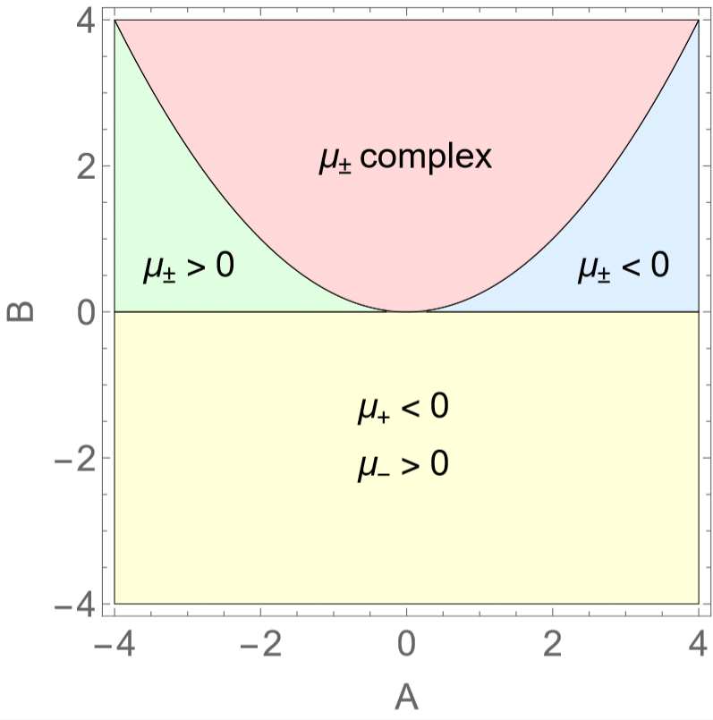
Figure 1: The properties of the masses $\mu_{\pm}$ in the parameter space $(A,B)$ are displayed.

We can state in brief, that when we perturb the metric tensor, the equation that describes the perturbation in the Ricci scalar is a fourth-order massive wave equation with two different masses. However, since the Ricci scalar perturbation depends on second-order derivatives of the metric perturbation, we would expect to be confronted with a six-order differential equation involving $\delta g_{ab}$, with a very complicated and untreatable form. The use of the Lorenz gauge is what enables one to reduce this equation to a fourth-order equation for a massive spin-0 degree of freedom. This fourth-order equation can be factorized into two commutative second-order equations of the form of a massive Klein-Gordon in general relativity. One can now apply the usual separation methods to expand the perturbation into spheroidal harmonics and a radial wavefunction. If wished one can use numerical integration techniques to compute the quasibound state frequencies.

IV The Kerr solution in GHMP: Equations, superradiant instabilities and stability regimes

IV.1 Separability of the equations of motion

IV.1.1 Separability of the equations of motion, quasibound state

Equations of the form (33) have been studied and are known to be separable for the Schwarzschild and Kerr metrics. We will be working with the Kerr metric, knowing that the Schwarzschild metric can be directly obtained from the Kerr metric by taking the limit where the angular momentum is equal to zero. The Kerr metric in Boyer-Lindquist coordinates $(t,r,\theta,\phi)$ is given by

$$ds^{2}=-\left(1-\frac{2Mr}{\rho^{2}}\right)dt^{2}+\frac{\rho^{2}}{\Delta}dr^{2}+\rho^{2}d\theta^{2}$$

$$-\frac{4Mra\sin^{2}\theta}{\rho^{2}}dtd\phi$$

$$+\left(r^{2}+a^{2}+\frac{2Mra^{2}\sin^{2}\theta}{\rho^{2}}\right)d\phi^{2},$$ (34)

with

$$\Delta=r^{2}+a^{2}-2Mr,\quad\rho^{2}=r^{2}+a^{2}\cos^{2}\theta,\quad a=\frac{J}{M},$$ (35)

where $M$ is the black hole mass and $J$ is the black hole angular momentum. The event horizon of the Kerr black hole is at the radius $r_{+}$ given by

$$r_{+}=M+\sqrt{M^{2}-a^{2}}\,.$$ (36)

To study the separability of the equations of motion, we first note that Eq. (31) is a fourth-order partial differential equation (PDE) for $\delta R$, and should therefore have four linearly independent solutions. The equation $\left(\Box-\mu_{+}^{2}\right)\delta R=0$ has two solutions, one solution corresponding to ingoing waves, the other corresponding to outgoing waves. Also, the equation $\left(\Box-\mu_{-}^{2}\right)\delta R=0$ has two solutions, one solution corresponding to ingoing waves, and the other corresponding to outgoing waves. To find these solutions we chose an ansatz of the form

$$\delta R=\psi\left(r\right)S\left(\theta\right)\exp\left(-i\omega t+im\phi\right),$$ (37)

where $\psi\left(r\right)$ is the radial wavefunction, $\omega$ is the wave angular frequency, $m$ is the azimuthal number, and $S\left(\theta\right)$ are the scalar spheroidal harmonics.

Using this ansatz, we can separate each of the factors $\left(\Box-\mu_{\pm}^{2}\right)\delta R=0$ into a radial and an angular equation. The angular equation is given by

$$\left[\lambda-m^{2}+a^{2}\left(\omega^{2}-\mu_{\pm}^{2}\right)\cos^{2}\theta\right]\sin^{2}\theta S\left(\theta\right)$$

$$+\sin\theta\partial_{\theta}\left[\sin\theta\partial_{\theta}S\left(\theta\right)\right]=0\,,$$ (38)

where $\lambda=l\left(l+1\right)+f\left(c\right)$, $l$ is the angular momentum number, $c=a^{2}\left(\omega^{2}-\mu_{\pm}^{2}\right)$ is a constant, and $f(c)$ is some function of $c$ that in the regime we are working is negligible $f(c)={\mathcal{O}}(c)$ with $c\ll 1$ as we will show. In this case, thus, the spheroidal harmonics can be approximated by the spherical harmonics, with a constant of separation $\lambda=l\left(l+1\right)$.

Using Eq. (38) in Eq. (33) one finds a radial equation for the radial wave function $\psi\left(r\right)$. To find a more suitable way to write this radial equation, it is useful to redefine the radial coordinate $r$ and the radial wave function $\psi\left(r\right)$. Let us define the tortoise coordinate $r_{*}$ and a new radial wavefunction $u\left(r\right)$ as

$$\frac{dr}{dr_{*}}=\frac{\Delta}{r^{2}+a^{2}},\qquad u\left(r\right)=\sqrt{r^{2}+a^{2}}\,\psi\left(r\right),$$ (39)

so that the new radial equation can be written in the form of a wave equation in the presence of a potential barrier as

$$\frac{d^{2}u}{dr_{*}^{2}}+\left[\omega^{2}-V\left(r\right)\right]u=0,$$ (40)

where the potential is given by

$$V\left(r\right) =\frac{\Delta}{r^{2}+a^{2}}\left[\frac{\Delta+\Delta^{\prime}r}{\left(r^{2}+a^{2}\right)^{2}}-\frac{3r^{2}\Delta}{\left(r^{2}+a^{2}\right)^{3}}+\frac{1}{r^{2}+a^{2}}\times\right.$$ (41)

$$\left.\left(\mu_{\pm}^{2}r^{2}-\omega^{2}a^{2}+\frac{4Mram\omega}{\Delta}-\frac{m^{2}a^{2}}{\Delta}+\lambda\right)\right]\hskip-2.84544pt.$$

Equation (40) admits two solutions, one corresponding to an ingoing wave and one to an outgoing wave. Due to the complicated form of the potential $V\left(r\right)$ of Eq. (41), Eq. (40) has no direct analytical solution and we resort to solving the equation numerically. For that we impose appropriate boundary conditions at the horizon, where $r=r_{+}$ and $r_{*}=-\infty$, and at infinity, where $r=+\infty$ and $r_{*}=+\infty$.

IV.1.2 Quasibound states

At the horizon $r_{+}$ the potential in Eq. (41) takes the form $V\left(r_{+}\right)=\omega^{2}-\left(\omega-m\Omega\right)^{2}$, where $\Omega=\frac{a}{2Mr_{+}}$ is the angular velocity of the horizon itself. Thus, Eq. (40) is $\frac{d^{2}u}{dr_{*}^{2}}+\left(\omega-m\Omega\right)^{2}u=0$. The solution is $u\left(r\right)=A_{+}e^{i\left(\omega-m\Omega\right)r_{*}}+B_{+}e^{-i\left(\omega-m\Omega\right)r_{*}}$, for some constants of integration $A_{+}$ and $B_{+}$. Since the horizon functions as a one-directional membrane, we want our boundary condition at the horizon to be given by a purely ingoing wave, i.e., at the horizon there are no outgoing waves, so the corresponding $A_{+}$ is zero, $A_{+}=0$. The solution is then $u\left(r\to r_{+}\right)=B_{+}e^{-i\left(\omega-m\Omega\right)r_{*}}$. At infinity the potential in Eq. (41) takes the form $V\left(\infty\right)=\mu_{\pm}^{2}$. Thus, Eq. (40) is $\frac{d^{2}u}{dr_{*}^{2}}+\left(\omega^{2}-\mu_{\pm}^{2}\right)u=0$. The solution is $u\left(r\right)=A_{\infty}e^{i\sqrt{\omega^{2}-\mu_{\pm}^{2}}r}+B_{\infty}e^{-i\sqrt{\omega^{2}-\mu_{\pm}^{2}}r}$, for some constants of integration $A_{\infty}$ and $B_{\infty}$. At infinity we want the solution to decay exponentially to give rise to a quasibound state, i.e., at infinity we want no waves and a decaying solution, so $\omega^{2}<\mu_{\pm}^{2}$ and $B_{\infty}=0$. The solution is then $u\left(r\to\infty\right)=A_{\infty}e^{-\sqrt{\mu_{\pm}^{2}-\omega^{2}}r}$. In brief, at the horizon and at infinity the solutions are

$$u\left(r\to r_{+}\right)=B_{+}e^{-i\left(\omega-m\Omega\right)r_{*}},$$

$$u\left(r\to\infty\right)=A_{\infty}e^{-\sqrt{\mu_{\pm}^{2}-\omega^{2}}r},$$ (42)

respectively.

Finding the quasibound states consists of integrating the radial Eq. (39) subjected to the boundary conditions in Eq. (42) and computing the roots for $\omega$. These roots will be of the form $\omega=\omega_{R}+i\omega_{I}$, with $\omega_{R}$ being the real part of the frequency and $\omega_{I}$ its imaginary part. As can be seen from Eq. (37), if $\omega_{I}<0$ the perturbation decays exponentially with time, but if $\omega_{I}>0$ the wavefunction grows exponentially and at some later time can no longer be considered a perturbation. These frequencies have been calculated in several places teukolsky1974 and we will not do it here. We want to study the instability and the stability of Kerr black holes in GHMP theory, so we proceed to such an analysis.

IV.2 Superradiant stability regimes

IV.2.1 General considerations about stability

As explained, each of the terms $\left(\Box-\mu_{\pm}^{2}\right)\delta R=0$, see Eq. (33), gives rise to a set of two different solutions, corresponding to an ingoing and an outgoing wave. Since these terms commute in the full equation given by Eq. (31), the complete solution for this equation is given by a linear combination of the two sets of solutions for each of the $\mu_{\pm}^{2}$’s. Since Eq. (31) is a fourth-order equation, these four solutions represent all the possible solutions for the equation. As the masses $\mu_{\pm}$ are different in general, the two sets of solutions will form quasibound states for different ranges of the angular frequency $\omega$. Note that if one of the two sets of solutions is unstable, then the entire solution will also be unstable, even if the other set is stable. The case $\mu_{\pm}=0$ is special in the sense that the solutions will be decaying oscillating solutions and so there are no quasibound states. If the superradiant condition $\omega<m\Omega$ is not satisfied the solution will be automatically stable. Let us now show that it is still possible to have stability even if there is superradiance. In this case there are two ways the solution can be stable.

The first way to have stability even if there is superradiance is to consider massless perturbations, $\mu_{\pm}^{2}=0$. In this case, there might be superradiant modes, but quasibound states never form, and so clearly the perturbation is stable.

The second way to have stability even if there is superradiance is to have a stable quasibound state. So, in this case the solution obeys the superradiant condition, namely, $\omega<m\Omega$. The solution has to have quasibound states, so the conditions $\mu_{\pm}>0$ and $\omega^{2}<\mu_{\pm}^{2}$ hold. Thus, we have

$$\omega<{\rm min}(m\Omega,\mu_{\pm})\,.$$ (43)

Moreover, to have stable bound states it is a sufficient condition that $\mu_{\pm}$ obeys beyer

$$\mu_{\pm}>\mu_{c}\,,\quad\mu_{c}=m\Omega\sqrt{1+\frac{2M}{r_{+}}}\,.$$ (44)

We can also achieve stability for a combination of the two cases above, i.e., one of the masses might vanish and the other might be in the range $\mu>\mu_{c}$.

Note that since $m$ is an azimuthal number, it does not have an upper bound, and so one could argue that for any constant value of $\mu_{\pm}^{2}$, there is always a value of $m$ such that $\mu_{\pm}<\mu_{c}$. However, it has been shown that superradiant instabilities are exponentially suppressed for larger values of $m$. This implies that we can consider an upper bound on $m$ for which the instability timescale is greater than the age of the Universe, say $m^{\rm max}$, and only after we choose an appropriate value of $\mu_{\pm}$ that satisfies the inequality $\mu_{\pm}>\mu_{c}^{\text{max}}$. This guarantees that even if the instabilities occur, their effects would not be seen.

IV.2.2 Stability regimes: Sufficient conditions on $f(R,\mathcal{R})$

A. The case $\mu_{\pm}^{2}=0$:

Let us start by studying the case where the masses $\mu_{\pm}^{2}$ vanish, $\mu_{\pm}^{2}=0$, which implies that quasibound states can never form and hence no instabilities can occur. From Eqs. (28) and (III.2), we verify that if both $A$ and $B$ vanish, then Eq. (31) becomes simply $\Box^{2}\delta R=0$. This corresponds to the origin of the plot in Fig. 1. If we can find a form of the function $f(R,\mathcal{R})$ such that both $A$ and $B$ vanish, then the Kerr solution will always be stable in this $f(R,\mathcal{R})$ theory.

To guarantee that none of the equations of motion diverge, we need to guarantee that all the first and second derivatives of $f$, i.e. $f_{R}$, $f_{\mathcal{R}}$, $f_{RR}$, $f_{\mathcal{R}\mathcal{R}}$, $f_{R\mathcal{R}}$, are finite. On the other hand, the factors $A$ and $B$, given by Eqs. (29) and (30), will vanish if the following conditions are satisfied, $f_{R\mathcal{R}}^{2}-f_{RR}f_{\mathcal{R}\mathcal{R}}\neq 0$, $f_{R}f_{\mathcal{R}\mathcal{R}}-2f_{\mathcal{R}}f_{R\mathcal{R}}-f_{\mathcal{R}}f_{RR}=0$, and $f_{R}+f_{\mathcal{R}}=0$. Note that these conditions must be satisfied at $R=\mathcal{R}=0$. There are many different functions $f$ that satisfy these conditions. The simplest class of functions $f$ that satisfies these conditions is

$$f(R,\mathcal{R})=\left(a_{1}+a_{2}R+a_{3}\mathcal{R}\right)\left(R-\mathcal{R}\right)$$ (45)

where $a_{1}$, $a_{2}$, and $a_{3}$ are constants that must satisfy the constraint $a_{2}\neq-a_{3}$. Any higher-order form of the function $f(R,\mathcal{R})$ obtained from Eq. (45) by adding terms such as $R^{3}$ or $R^{2}\mathcal{R}$ will also have stable solutions because all these extra terms vanish when we set $R=0$ and $\mathcal{R}=0$ in Eqs. (29) and (30).

B. The case $\mu_{-}=0$ with $\mu_{+}>\mu_{c}$:

Here we want $\mu_{-}=0$ with $\mu_{+}>\mu_{c}$. As can be seen from Eq. (III.2), the only way for $\mu_{-}=0$ is to have $B=0,\,A>0$, but these constraints impose that $\mu_{+}<0$, see Fig. 1, so $\mu_{+}$ can never be greater than $\mu_{c}$. So there are no forms of $f(R,\mathcal{R})$ for which the conditions $\mu_{-}=0$ with $\mu_{+}>\mu_{c}$ are satisfied.

C. The case $\mu_{+}=0$ with $\mu_{-}>\mu_{c}$:

Let us now set $\mu_{+}=0$ by choosing $B=0,A<0$, and in this region we have $\mu_{-}>0$, see Fig. 1, and we have to see whether we can choose the function $f$ in such a way that $\mu_{-}>\mu_{c}$ or not.

As before, in order to avoid divergences in the equations of motion we have to guarantee that all the first and second derivatives of $f$, i.e. $f_{R}$, $f_{\mathcal{R}}$, $f_{RR}$, $f_{\mathcal{R}\mathcal{R}}$, $f_{R\mathcal{R}}$, are finite, and the extra constraints on the function $f$ such that $B=0$ and $A\neq 0$ are $f_{R\mathcal{R}}^{2}-f_{RR}f_{\mathcal{R}\mathcal{R}}\neq 0$, $f_{R}f_{\mathcal{R}\mathcal{R}}-2f_{\mathcal{R}}f_{R\mathcal{R}}$, and $f_{R}+f_{\mathcal{R}}=0$. These conditions must be satisfied at $R=\mathcal{R}=0$. A simple class of functions $f$ that satisfies these constraints is

$$f(R,\mathcal{R})=a_{1}(R-\mathcal{R})+a_{2}R^{2}+a_{3}\mathcal{R}^{2}+a_{4}R\mathcal{R},$$ (46)

where $a_{1}$, $a_{2}$, $a_{3}$, and $a_{4}$ are constants. This form of the function $f$ implies, by Eqs. (29), (30) and (III.2), that $\mu_{-}$ and $A$ can be written as

$$\mu_{-}=-A=\frac{2a_{1}\left(a_{2}+a_{3}+a_{4}\right)}{12a_{2}a_{3}-3a_{4}^{2}}\,.$$ (47)

In order that the solutions are stable we have to guarantee that the $\mu_{-}$ of Eq. (47) is greater than $\mu_{c}$, i.e., $\frac{2a_{1}\left(a_{2}+a_{3}+a_{4}\right)}{12a_{2}a_{3}-3a_{4}^{2}}>\mu_{c}$. To obtain a finite $A$, and thus a finite $\mu_{-}$, both the numerator and the denominator of Eq. (47) must be $\neq 0$. Now, let us try to find a specific combination of the constants $a_{1}$, $a_{2}$, $a_{3}$, and $a_{4}$ such that $\mu_{-}>\mu_{c}$ is satisfied. There are many combinations that work, but let us take for example the case where $a_{3}$ and $a_{4}$ are set and verify if there is a value of $a_{2}$ that solves the problem. Note that the denominator of Eq. (47) diverges to $+\infty$ when we take the limit $a_{2}\to a_{4}^{2}/\left(4a_{3}\right)$ from above. Also, if we choose both $a_{3}>0$ and $a_{4}>0$, then $a_{2}>0$ and the numerator of Eq. (47) is positive in this limit. This implies that we can always choose a finite value of $a_{2}\gtrsim a_{4}^{2}/\left(4a_{3}\right)$ arbitrarily close to $a_{4}^{2}/\left(4a_{3}\right)$ such that for any $m$ and $\Omega$ the condition $\mu_{-}>\mu_{c}$ is always satisfied. Note that $m$ does not have an upper limit, but since superradiant instabilities are exponentially suppressed for larger values of $l$ and $m$, one has that for $m\gg 1$ the effects of these instabilities are negligible. Again, any higher-order form of the function $f(R,\mathcal{R})$ will also have stable solutions because all these extra terms vanish when we set $R=0$ and $\mathcal{R}=0$ in Eqs. (29) and (30).

D. The case $\mu_{\pm}>\mu_{c}$:

Finally, we turn to the case where both masses are $\mu_{\pm}>\mu_{c}$. In this case we need both $A$ and $B$ to be finite. Let us analyze the regions of the parameter space of $A$ and $B$ that allow for these solutions to exist. From Eq. (III.2) and Fig. 1, we can see that there are three regions of the phase space that must be excluded: 1. Region $4B>A^{2}$, because both $\mu_{\pm}^{2}$ are complex; 2. Region $B<0$, because $\mu_{+}$ is always negative; 3. Region $B>0$ and $A>0$, because both $\mu_{\pm}^{2}$ are negative. We are then constrained to work in the region defined by the three conditions $B>0$, $A<0$ and $A^{2}>4B$.

The approach to this problem is different from the previous ones. Let us first study the structure of the $\mu_{\pm}^{2}$ as functions of $A$ and $B$ in Eq. (III.2). In the limit of large $\mu_{\pm}^{2}$, we must have $A\to-\infty$ like in the previous case. However, in this limit, the quantity inside the square root is going to depend on how $B$ is proportional to $A$. If $B\propto|A|^{n}$ with $n<2$, then in this limit $\sqrt{A^{2}-4B}\to|A|$ and $\mu_{+}\to 0$, and we recover the previous case. On the other hand, if $B\propto|A|^{n}$ with $n>2$, then in this limit we eventually break the relation $A^{2}>4B$ and the $\mu_{\pm}^{2}$ become complex. Therefore, we need a behavior of $B$ of the form $B=CA^{2}$ for some constant $C$. Then, the constraints $B>0$ and $A^{2}>4B$ imply that the constant $C$ must be somewhere in the region $0<C<1/4$. Inserting this form of $B$ into Eq. (III.2) leads to the relation $\mu_{\pm}^{2}=-(1/2)A\left(1\mp\sqrt{1-4C}\right)>0$, where the inequality arises since we know that $A<0$ and $C<1/4$. At this point, if we can choose a specific form of the function $f$ such that we can make $A$ arbitrarily large, our problem is solved. Also note that in the limit $C=0$ we recover the previous case C where $\mu_{+}=0$, and in the limit $C=1/4$ we obtain $\mu_{+}=\mu_{-}$ which can be shown to give $\mu_{+}=\mu_{-}=0$ recovering case A, i.e., $\mu_{\pm}^{2}=0$.

Consider now the most general form of the function $f$ that avoids divergences in the equations of motion, i.e., a function $f$ for which $f_{R}$, $f_{\mathcal{R}}$, $f_{RR}$, $f_{\mathcal{R}\mathcal{R}}$ and $f_{R\mathcal{R}}$ are finite,

$$f(R,\mathcal{R})=a_{1}R+a_{2}\mathcal{R}+a_{3}R^{2}+a_{4}\mathcal{R}^{2}+a_{5}R\mathcal{R},$$ (48)

where $a_{1}$, $a_{2}$, $a_{3}$, $a_{4}$, and $a_{5}$, are constants assumed different from zero. For this particular choice of $f$, we see by Eq. (30) that $A$ diverges to $-\infty$ if the numerator is positive and we take the limit $a_{3}\to a_{5}^{2}/\left(4a_{4}\right)$ from above, or if the numerator is negative and we take the limit $a_{3}\to a_{5}^{2}/\left(4a_{4}\right)$ from below. However, this is not enough to conclude that we can make $\mu_{\pm}^{2}$ arbitrarily large. We also need to verify that $B=CA^{2}$, with $0<C<1/4$, i.e., from Eq. (30) we must have $f_{\mathcal{R}}\left(f_{\mathcal{R}}+f_{R}\right)\left(f_{\mathcal{R}R}^{2}-f_{RR}f_{\mathcal{R}\mathcal{R}}\right)=C\big{(}f_{R}f_{\mathcal{R}\mathcal{R}}-2f_{\mathcal{R}}f_{\mathcal{R}R}-f_{\mathcal{R}}f_{RR}\big{)}^{2}$ with $f_{\mathcal{R}R}^{2}-f_{RR}f_{\mathcal{R}\mathcal{R}}\neq 0$. Finding the most general combinations of $a_{1}$, $a_{2}$, $a_{3}$, $a_{4}$, and $a_{5}$, for which the function $f$ satisfies these constraints is a fine-tuning problem. To solve this problem we proceed as follows. First we write $a_{3}=a_{5}^{2}/\left(4a_{4}\right)+\epsilon$, for some $\epsilon\gtrsim 0$ that must be finite but we can make it arbitrarily small. We also need to have $a_{2}\neq a_{1}$ to guarantee that $B\neq 0$, so it is better to redefine $a_{2}$ as an $a_{6}$ given by $a_{2}\equiv-\left(a_{6}+1\right)a_{1}$, where $a_{6}\neq 0$. Inserting these considerations into $f_{\mathcal{R}}\left(f_{\mathcal{R}}+f_{R}\right)\left(f_{\mathcal{R}R}^{2}-f_{RR}f_{\mathcal{R}\mathcal{R}}\right)=C\big{(}f_{R}f_{\mathcal{R}\mathcal{R}}-2f_{\mathcal{R}}f_{\mathcal{R}R}-f_{\mathcal{R}}f_{RR}\big{)}^{2}$, we verify that $C$ is positive in the small-$\epsilon$ limit only if the condition $a_{4}a_{6}\left(1+a_{6}\right)<0$. This happens in the regimes $-1<a_{6}<0$ with $a_{4}>0$, $a_{6}<-1$ with $a_{4}<0$, and $a_{6}>0$ with $a_{4}<0$. As an example, let us consider $a_{4}=1$, and then $a_{6}=-1/2$ which corresponds to the maximum of the polynomial $-a_{6}\left(a_{6}+1\right)$. Finally, we have to guarantee that $A<0$ in this regime. Inserting these results into Eq. (29) we verify that $A<0$ requires that the quantities $\left(a_{5}+1\right)$ and $a_{1}$ have the same sign. For simplicity, let us take $a_{1}=a_{5}=1$. So in this example we have $a_{1}=1$, $a_{1}=-\frac{1}{2}$, $a_{3}=\frac{1}{4}+\epsilon$, $a_{4}=1$, and $a_{5}=1$. Note that other choices for the values of the parameters $a_{1}$, $a_{2}$, $a_{3}$, $a_{4}$, and $a_{5}$, could also be made following the same reasoning. Here, our aim is simply to provide an example of a combination that works. We are thus left with

$$\mu_{\pm}^{2}=-\frac{A}{2}\left(1\mp\sqrt{1-4C}\right)\,,\quad$$

$$A=-\frac{13+4\epsilon}{48\epsilon}\,,\quad C=\frac{16\epsilon}{\left(13+4\epsilon\right)^{2}}\,,$$ (49)

From these results, we verify that for any $\epsilon>0$ we have, $0<C<1/4$, and also that in the limit $\epsilon\to 0$ we have $A\to-\infty$ and thus $\mu^{2}_{\pm}\to+\infty$. We can thus consider $\epsilon$ arbitrarily small and force $\mu^{2}_{\pm}>\mu_{c}$ for any $m$ and $\Omega$. We note that $m$ does not have an upper bound, but superradiant instabilities are exponentially suppressed for large values of $m$ and we can neglect their effects. Again, any higher-order form of the function $f(R,\mathcal{R})$ will also work because the extra terms vanish for $R=\mathcal{R}=0$.

V Conclusions

Within GHMP with its generic function $f(R,\mathcal{R})$, we have shown that it is always possible to choose a specific value for $\mathcal{R}$, namely $\mathcal{R}=\mathcal{R}_{0}$ for some solution in general relativity with constant $R=0$ such that this solution is also a solution for the GHMP gravity for any form of the function $f$ that satisfies two very general conditions: $f$ must be analytical in the point $\{0,\mathcal{R}_{0}\}$, and $f$ must have a zero in the same point, i.e., $f\left(0,\mathcal{R}_{0}\right)=0$. Inserting this result into the field equations leads to the conclusion that $\mathcal{R}_{0}=0$. This result is in agreement with the fact that for constant $R$ and $\mathcal{R}$, the conformal factor between the metrics $g_{ab}$ and $h_{ab}$, which is given by $f_{\mathcal{R}}$, is constant and therefore both metrics $g_{ab}$ and $h_{ab}$ must have the same Ricci tensor.

We have extended the scrutiny of the GHMP gravity by studying which functions $f(R,\mathcal{R})$ yield stability against scalar perturbations of Kerr black hole solutions. The stability of the Kerr metric against superradiant instabilities is dictated by two conditions: either the masses of the perturbations vanish, $\mu_{\pm}=0$, or the masses of these perturbations exceed a critical value $\mu_{\pm}>\mu_{c}$. We have shown that it is possible to select specific well-behaved forms of the function $f$ such that one of these two conditions is satisfied for any value of the angular frequency $\omega$. Also, since the masses only depend on the values of $f$ and its derivatives at $R=\mathcal{R}=0$, any higher-order term on $R$ and $\mathcal{R}$ up to infinity can be added to the function $f$ leaving these results unaffected, being then coherent with the two general constraints we imposed on the function $f$ to begin with. It would be of interest to see the restrictions imposed on $f$ by vector and tensor perturbations of the Kerr solution.

Appendix A Scalar-tensor representation of GHMP gravity

The objective of this appendix is to show that one can perform the perturbative analysis in the scalar-tensor representation of the GHMP theory and that the perturbation equations and the results are the same. The scalar-tensor representation can be achieved by considering an action with two auxiliary fields, $\alpha$ and $\beta$, respectively, in the following form

$$S=\frac{1}{2\kappa^{2}}\int_{\Omega}\sqrt{-g}\Big{[}f\left(\alpha,\beta\right)+\frac{\partial f}{\partial\alpha}\left(R-\alpha\right)$$

$$+\frac{\partial f}{\partial\beta}\left(\cal{R}-\beta\right)\Big{]}d^{4}x+S_{m}.$$ (50)

Using $\alpha=R$ and $\beta=\mathcal{R}$ we recover the initial action in Eq. (1). Therefore, we can define two scalar fields as $\varphi=\partial f/\partial\alpha$ and $\psi=-\partial f/\partial\beta$, where the negative sign is set here for convention. The equivalent action is of the form

$$S=\frac{1}{2\kappa^{2}}\int_{\Omega}\sqrt{-g}\left[\varphi R-\psi\mathcal{R}-V\left(\varphi,\psi\right)\right]d^{4}x,$$ (51)

where we defined the potential $V$ as

$$V\left(\varphi,\psi\right)=-f\left(\alpha,\beta\right)+\varphi\alpha-\psi\beta.$$ (52)

We now have an action with four independent variables, namely the metric $g_{ab}$, the independent connection $\hat{\Gamma}$, and the scalar fields $\varphi$ and $\psi$. The equation of motion for $\hat{\Gamma}$ remains the same as in the geometrical representation and it is given by Eq. (5) or, equivalently, by Eq. (8). Using the definitions of the scalar fields, this now becomes

$$\mathcal{R}_{ab}=R_{ab}-\frac{1}{\psi}\left(\nabla_{a}\nabla_{b}+\frac{1}{2}g_{ab}\Box\right)\psi+\frac{3}{2\psi^{2}}\partial_{a}\psi\partial_{b}\psi.$$ (53)

Varying Eq. (51) with respect to the metric $g_{ab}$ yields the field equation

$$\varphi R_{ab}-\psi\mathcal{R}_{ab}-\frac{1}{2}g_{ab}\left(\varphi R-\psi\mathcal{R}-V\right)-$$

$$-\left(\nabla_{a}\nabla_{b}-g_{ab}\Box\right)\varphi=0,$$ (54)

where we used the fact that $T_{ab}=0$ for the solutions in which we are interested in this paper. This equation is in agreement with the geometrical representation in the sense that it can be obtained from Eq. (II) simply by using the definitions of the scalar fields $\varphi$, $\psi$, and the potential $V$. Finally, varying the action in Eq. (51) with respect to the scalar fields $\varphi$ and $\psi$ yields directly

$$R=V_{\varphi},\ \ \ \ \ \mathcal{R}=-V_{\psi},$$ (55)

where the subscripts $\varphi$ and $\psi$ denote derivatives with respect to the scalar fields $\varphi$ and $\psi$, respectively.

Using Eq. (53) and its trace to cancel the terms $\mathcal{R}_{ab}$ and $\mathcal{R}$ in Eq. (51), and tracing the result, one verifies that one of the possible ways for a solution in general relativity with $R=0$ to be a solution for this representation of the GHMP gravity is to impose that $V=0$ and also that both scalar fields $\varphi$ and $\psi$ are constants. Note that the trace of the field equation is a PDE for $\varphi$ and $\psi$, like in Sec. III where it was a PDE for $\mathcal{R}$, and therefore these solutions are not unique. We choose constant scalar fields as solutions because this is equivalent to setting $\mathcal{R}=\mathcal{R}_{0}$ for some constant $\mathcal{R}_{0}$, and we recover the results of the geometrical representation. Then, using $\psi=\psi_{0}$ for some constant $\psi_{0}$ in the trace of Eq. (53) one verifies that $\mathcal{R}=R=0$, which is the same result we obtained before. The constraint $V=0$, for solutions with $\mathcal{R}=R=0$ is equivalent to the constraint $f\left(0,0\right)=0$ that we obtained in Sec. III. On the other hand, constraining $\varphi$ and $\psi$ to be constants is equivalent to constraining $f_{R}$ and $f_{\mathcal{R}}$ to be constants in the geometrical representation, which is exactly what happens for $\mathcal{R}=R=0$, and thus these results are consistent with the ones from Sec. III.

Now, let us perturb the metric $g_{ab}$ in the same way we did in Eq. (17). This will again impose a perturbation in both $R$ and $\mathcal{R}$ of the forms $R=\bar{R}+\epsilon\delta R$ and $\mathcal{R}=\bar{\mathcal{R}}+\epsilon\delta\mathcal{R}$, plus additional perturbations of the scalar fields of the form $\varphi=\bar{\varphi}+\epsilon\delta\varphi$ and $\psi=\bar{\psi}+\epsilon\delta\psi$. From the definitions of the scalar fields and using the fact that $\alpha=R$ and $\beta=\mathcal{R}$, we can rewrite the perturbations in the scalar fields as

$$\delta\varphi=\frac{\partial^{2}f}{\partial\alpha^{2}}\delta\alpha+\frac{\partial^{2}f}{\partial\alpha\partial\beta}\delta\beta=\bar{f}_{RR}\delta R+\bar{f}_{R\mathcal{R}}\delta\mathcal{R},$$ (56)

$$\delta\psi=\frac{\partial^{2}f}{\partial\beta^{2}}\delta\beta+\frac{\partial^{2}f}{\partial\beta\partial\alpha}\delta\alpha=\bar{f}_{\mathcal{R}\mathcal{R}}\delta\mathcal{R}+\bar{f}_{\mathcal{R}R}\delta R.$$ (57)

Inserting these perturbations into the traces of Eqs. (53) and (54) and keeping only the terms to leading order in $\epsilon$ yields again the same equations as Eqs. (26) and (27), and the procedure is the same as that in Sec. III. We therefore conclude that the analysis of metric perturbations in both representations of the theory is equivalent, as anticipated.

References

- (1) C. Misner, K. S. Thorne, and J. A. Wheeler, Gravitation (Freeeman, San Francisco, 1973).
- (2) T. P. Sotiriou and V. Faraoni, “ theories of gravity”, Rev. Mod. Phys. 82, 451 (2010); arXiv:0805.1726 [gr-qc].
- (3) A. De Felice and S. Tsujikawa, “ theories”, Living Rev. Relativity 13, 3 (2010); arXiv:1002.4928 [gr-qc].
- (4) S. Nojiri and S. D. Odintsov, “Unified cosmic history in modified gravity: From theory to Lorentz non-invariant models”, Phys. Rep. 505, 59 (2011); arXiv:1011.0544 [gr-qc].
- (5) S. Capozziello and M. De Laurentis, “Extended theories of gravity”, Phys. Rep. 509, 167 (2011); arXiv:1108.6266 [gr-qc].
- (6) G. J. Olmo, “Palatini approach to modified gravity: theories and beyond”, Int. J. Mod. Phys. D 20, 413 (2011); arXiv:1101.3864 [gr-qc].
- (7) T. Harko, T. S. Koivisto, F. S. N. Lobo, and G. J. Olmo, “Metric-Palatini gravity unifying local constraints and late-time cosmic acceleration”, Phys. Rev. D 85, 084016 (2012); arXiv:1110.1049 [gr-qc].
- (8) S. Capozziello, T. Harko, T. S. Koivisto, F. S. N. Lobo, and G. J. Olmo, “Hybrid metric-Palatini gravity”, Universe 1, 199 (2015); arXiv:1508.04641 [gr-qc].
- (9) S. Capozziello, T. Harko, T. S. Koivisto, F. S. N. Lobo, and G. J. Olmo, “Cosmology of hybrid metric-Palatini f(X)-gravity”, J. Cosmol. Astropart. Phys. (JCAP) 04 (2013) 011; arXiv:1209.2895 [gr-qc].
- (10) S. Capozziello, T. Harko, T. S. Koivisto, F. S. N. Lobo, and G. J. Olmo, “Galactic rotation curves in hybrid metric-Palatini gravity”, Astropart. Phys. 50-52, 65 (2013); arXiv:1307.0752 [gr-qc].
- (11) S. Capozziello, T. Harko, T. S. Koivisto, F. S. N. Lobo, and G. J. Olmo, “The virial theorem and the dark matter problem in hybrid metric-Palatini gravity”, J. Cosmol. Astropart. Phys. (JCAP) 07 (2013) 024; arXiv:1212.5817 [physics.gen-ph].
- (12) T. Harko and F. S. N. Lobo, Extensions of Gravity: Curvature-Matter Couplings and Hybrid Metric-Palatini Theory (Cambridge University Press, Cambridge 2018).
- (13) N. Tamanini and C. G. Bohmer, “Generalized hybrid metric-Palatini gravity”, Phys. Rev. D 87, 084031 (2013); arXiv:1302.2355 [gr-qc].
- (14) J. L. Rosa, S. Carloni, J. P. S. Lemos, and F. S. N. Lobo, “Cosmological solutions in generalized hybrid metric-Palatini gravity”, Phys. Rev. D 95, 124035 (2017); arXiv:1703.03335 [gr-qc].
- (15) J. L. Rosa, J. P. S. Lemos, and F. S. N. Lobo, “Wormholes in generalized hybrid metric-Palatini gravity obeying the matter null energy condition everywhere”, Phys. Rev. D 98, 064054 (2018); arXiv:1808.08975 [gr-qc].
- (16) R. P. Kerr, “Gravitational field of a spinning mass as an example of algebraically special metrics”, Phys. Rev. Lett. 11, 237 (1963).
- (17) S. A. Teukolsky, “Perturbations of a rotating black holes. III. Interaction of the hole with gravitational and electromagnetic radiation”, Astrophys. J. 193, 443 (1974).
- (18) S. Chandrasekhar, The Mathematical Theory of Black Holes (Clarendon Press, Oxford, 1983).
- (19) H. R. Beyer, “On the stability of the massive scalar field in Kerr space-time”, J. Math. Phys. 52, 102502 (2011); arXiv:1105.4956 [math-ph].
- (20) W. H. Press and S. A. Teukolsky, “Floating orbits, superradiant scattering and the black-hole bomb”, Nature 238, 211 (1972).
- (21) V. Cardoso, O. J. C. Dias, J. P. S. Lemos, and S. Yoshida, “The black hole bomb and superradiant instabilities”, Phys. Rev. D 70, 044039 (2004); arXiv:hep-th/0404096.
- (22) Y. S. Myung, T. Moon, and E. J. Son, “Stability of black holes”, Phys. Rev. D 83, 124009 (2011); arXiv:1103.0343 [gr-qc].
- (23) T. Moon, Y. S. Myung, and E. J. Son, “Stability analysis of -AdS black holes”, Eur. Phys. J. C 71, 1777 (2011); arXiv:1104.1908 [gr-qc].
- (24) T. Moon and Y. S. Myung, “Stability of Schwarzschild black hole in gravity with the dynamical Chern-Simons term”, Phys. Rev. D 84, 104029 (2011); arXiv:1109.2719 [gr-qc].
- (25) Y. S. Myung, “Stability of Schwarzschild black holes in fourth-order gravity revisited”, Phys. Rev. D 88, 024039 (2013); arXiv:1306.3725 [gr-qc].
- (26) Y. S. Myung and Y. J. Park, “Stability issues of black hole in non-local gravity”, Phys. Lett. B 779, 342 (2018); arXiv:1711.06411 [gr-qc].
- (27) Y. S. Myung, “Instability of rotating black hole in a limited form of gravity”, Phys. Rev. D 84, 024048 (2011); arXiv:1104.3180 [gr-qc].
- (28) Y. S. Myung, “Instability of a Kerr black hole in gravity”, Phys. Rev. D 88, 104017 (2013); arXiv:1309.3346 [gr-qc].