Directed searches for continuous gravitational waves from twelve supernova remnants in data from Advanced LIGO’s second observing run
Abstract
We describe directed searches for continuous gravitational waves from twelve well localized non-pulsing candidate neutron stars in young supernova remnants using data from Advanced LIGO’s second observing run. We assumed that each neutron star is isolated and searched a band of frequencies from 15 to 150 Hz, consistent with frequencies expected from known young pulsars. After coherently integrating spans of data ranging from 12.0 to 55.9 days using the -statistic and applying data-based vetoes, we found no evidence of astrophysical signals. We set upper limits on intrinsic gravitational wave amplitude in some cases stronger than generally about a factor of two better than upper limits on the same objects from Advanced LIGO’s first observing run.
I Introduction
Young isolated neutron stars and suspected locations of the same are promising targets for directed searches for continuous gravitational waves Glampedakis and Gualtieri (2018). Even without timing obtained from electromagnetic observations of a pulsar, such searches can achieve interesting sensitivities for reasonable computational costs Wette et al. (2008). Young supernova remnants containing candidate non-pulsing neutron stars are natural targets for such searches, as are small SNRs or pulsar wind nebulae even in the absence of a candidate neutron star (as long as the SNR is not Type Ia, which does not leave behind a compact object).
Many upper limits on continuous GWs from isolated, well localized neutron stars other than known pulsars have been published over the last decade. These have used data ranging from Initial LIGO runs to Advanced LIGO’s first observing run (O1) and second observing run (O2). Most searches targeted relatively young SNRs Abadie et al. (2010, 2011); Aasi et al. (2015); Sun et al. (2016); Zhu et al. (2016); Abbott et al. (2017a, 2019a); Ming et al. (2019); Abbott et al. (2019b). Some searches targeted promising small areas such as the galactic center Abadie et al. (2011); Aasi et al. (2013); Abbott et al. (2017a, 2019b); Piccinni et al. (2019). One search targeted a nearby globular cluster, where multi-body interactions might effectively rejuvenate an old neutron star for purposes of continuous GW emission Abbott et al. (2017b). Some searches used short coherence times and fast, computationally cheap methods originally developed for the stochastic GW background Abadie et al. (2011); Abbott et al. (2017a, 2019b). Most searches were slower but more sensitive, using longer coherence times and methods specialized for continuous waves based on matched filtering and similar techniques.
Here we present the first searches of O2 data for twelve SNRs, using the fully coherent -statistic as implemented in a code pipeline descended from the one used in the first published search Abadie et al. (2010) among others Aasi et al. (2015); Abbott et al. (2019a). Since the O2 noise spectrum is not much lower than O1, we deepened these searches with respect to O1 searches Abbott et al. (2019a) by focusing on low frequencies compatible with those observed in young pulsars Manchester et al. (2005). This focus allowed us to increase coherence times and obtain significant improvements in sensitivity over O1. Low frequencies have the drawback, however, that greater neutron star ellipticities or -mode amplitudes are required to generate detectable signals. We did not search three SNRs from the list in Ref. Abbott et al. (2019a) because the Einstein@Home distributed computing project has already searched them Ming et al. (2019) to a depth which cannot be matched without such great computing resources which we do not have. We also did not search Fomalhaut b as in Ref. Abbott et al. (2019a) because our code (although improved over previous versions) is inefficient for targets with such long spin-down timescales. In the future we plan to improve the code to efficiently search higher frequencies and longer spin-down timescales. For now our searches are interesting as the most sensitive yet (in strain) for these twelve SNRs.
II Searches
| SNR | parameter | Other name | RA+dec | Ref. | Ref. | Ref. | ||
|---|---|---|---|---|---|---|---|---|
| (G name) | space | (J2000 h:m:s+d:m:s) | (kpc) | (kyr) | ||||
| 1.9+0.3 | — | 17:48:46.9−27:10:16 | Reich et al. (1984) | Reynolds et al. (2008) | Reynolds et al. (2008) | |||
| 15.9+0.2 | wide | — | 18:18:52.1−15:02:14 | Reynolds et al. (2006) | Reynolds et al. (2006) | Reynolds et al. (2006) | ||
| 15.9+0.2 | deep | — | 18:18:52.1−15:02:14 | Reynolds et al. (2006) | Reynolds et al. (2006) | Reynolds et al. (2006) | ||
| 18.9−1.1 | — | 18:29:13.1−12:51:13 | Tüllmann et al. (2010) | Harrus et al. (2004) | Harrus et al. (2004) | |||
| 39.2−0.3 | 3C 396 | 19:04:04.7+05:27:12 | Olbert et al. (2003) | Su et al. (2011) | Su et al. (2011) | |||
| 65.7+1.2 | DA 495 | 19:52:17.0+29:25:53 | Arzoumanian et al. (2008) | Kothes et al. (2004) | Kothes et al. (2008) | |||
| 93.3+6.9 | DA 530 | 20:52:14.0+55:17:22 | Jiang et al. (2007) | Foster and Routledge (2003) | Jiang et al. (2007) | |||
| 189.1+3.0 | wide | IC 443 | 06:17:05.3+22:21:27 | Olbert et al. (2001) | Fesen and Kirshner (1980) | Petre et al. (1988) | ||
| 189.1+3.0 | deep | IC 443 | 06:17:05.3+22:21:27 | Olbert et al. (2001) | Fesen and Kirshner (1980) | Swartz et al. (2015) | ||
| 291.0−0.1 | MSH 11−62 | 11:11:48.6−60:39:26 | Slane et al. (2012) | Moffett et al. (2001) | Slane et al. (2012) | |||
| 330.2+1.0 | wide | — | 16:01:03.1−51:33:54 | Park et al. (2006) | McClure-Griffiths et al. (2001) | Park et al. (2009) | ||
| 330.2+1.0 | deep | — | 16:01:03.1−51:33:54 | Park et al. (2006) | McClure-Griffiths et al. (2001) | Torii et al. (2006) | ||
| 350.1−0.3 | — | 17:20:54.5−37:26:52 | Gaensler et al. (2008) | Gaensler et al. (2008) | Lovchinsky et al. (2011) | |||
| 353.6−0.7 | — | 17:32:03.3−34:45:18 | Halpern and Gotthelf (2010) | Tian et al. (2008) | Tian et al. (2008) | |||
| 354.4+0.0 | wide | — | 17:31:27.5−33:34:12 | Roy and Pal (2013) | Roy and Pal (2013) | Roy and Pal (2013) | ||
| 354.4+0.0 | deep | — | 17:31:27.5−33:34:12 | Roy and Pal (2013) | Roy and Pal (2013) | Roy and Pal (2013) |
In most respects the searches were done similarly to Abbott et al. (2019a), so we summarize briefly and refer the reader to that paper for further details. The same goes for the upper limits described in the next Section.
II.1 Setup
We made the usual assumptions about the signals, that they had negligible intrinsic amplitude evolution and that their frequency evolution in the frame of the solar system barycenter was given by
| (1) |
where is the beginning of the observation, the frequency derivatives are evaluated at that time, and we write a simple for Hence our searches were sensitive to neutron stars without binary companions, significant timing noise, or glitches; and spinning down on timescales much longer than the duration of any observation.
We used the multi-detector -statistic Jaranowski et al. (1998); Cutler and Schutz (2005), which combines matched filters for the above type of signal in such a way as to account for amplitude and phase modulation due to the daily rotation of the detectors with relatively little computational cost. In stationary Gaussian noise, is drawn from a distribution with four degrees of freedom. The is noncentral if a signal is present. For loud signals the amplitude signal-to-noise ratio is roughly
We used Advanced LIGO O2 data Vallisneri et al. (2015); Abbott et al. (2019c) with version C02 calibration and cleaning as described in Cahillane et al. (2018). Thus the amplitude calibration uncertainties were no greater than 8% for each interferometer. As in previous searches of this type, we used strain data processed into short Fourier transforms of 1800 s duration, high pass filtered and Tukey windowed. And we chose the set of SFTs for each search, once its time span was fixed (see below), by minimizing the harmonic mean of the noise power spectral density over the span and the frequency band.
With the direction to each candidate neutron star known, the parameter space of each search was the set In contrast to Ref. Abbott et al. (2019a) and earlier searches, we fixed and at 15 Hz and 150 Hz respectively. Our goal was to improve the sensitivity significantly over earlier O1 results Abbott et al. (2019a); Ming et al. (2019), even though the strain noise was only slightly improved, while focusing on a range of frequencies compatible with the emission expected from known young pulsars Manchester et al. (2005). Rounding up a bit from the 124 Hz expected from the fastest known young pulsar, we set to 150 Hz. Since the precise value of has very little effect on the cost of the searches, we somewhat arbitrarily set it to 15 Hz where the noise spectrum is rising steeply. The ranges of frequency derivatives were then chosen as in Abbott et al. (2019a), with
| (2) |
for a given and
| (3) |
for a given Thus we were open to a wide but physically motivated range of possible emission scenarios.
II.2 Target List
| SNR | parameter | Start of span | H1 | L1 | Duty | |||
|---|---|---|---|---|---|---|---|---|
| (G name) | space | (seconds) | (days) | (UTC, 2017) | SFTs | SFTs | factor | |
| 1.9+0.3 | 1,036,229 | 12.0 | Jun 23 03:59:29 | 460 | 466 | 0.80 | ||
| 15.9+0.2 | wide | 1,744,260 | 20.2 | Aug 04 21:11:52 | 753 | 748 | 0.77 | |
| 15.9+0.2 | deep | 2,593,109 | 30.0 | Jul 26 21:41:05 | 1076 | 1095 | 0.75 | |
| 18.9−1.1 | 3,014,418 | 34.9 | Jul 22 00:39:16 | 1204 | 1272 | 0.74 | ||
| 39.2−0.3 | 2,734,846 | 31.7 | Jul 23 17:19:34 | 1106 | 1152 | 0.74 | ||
| 65.7+1.2 | 4,450,430 | 51.5 | Jan 19 08:03:58 | 1916 | 1580 | 0.71 | ||
| 93.3+6.9 | 3,067,958 | 35.5 | Jul 21 08:46:56 | 1224 | 1288 | 0.74 | ||
| 189.1+3.0 | wide | 2,739,425 | 31.7 | Jul 23 16:03:15 | 1108 | 1154 | 0.74 | |
| 189.1+3.0 | deep | 4,468,104 | 51.7 | Jan 19 03:09:24 | 1917 | 1588 | 0.71 | |
| 291.0−0.1 | 2,160,350 | 25.0 | Jul 28 03:45:55 | 906 | 913 | 0.76 | ||
| 330.2+1.0 | wide | 2,056,663 | 23.8 | Aug 02 00:41:51 | 876 | 865 | 0.73 | |
| 330.2+1.0 | deep | 2,765,446 | 32.0 | Jul 23 08:49:34 | 1116 | 1169 | 0.74 | |
| 350.1−0.3 | 1,794,825 | 20.8 | Aug 05 03:25:49 | 777 | 773 | 0.78 | ||
| 353.6−0.7 | 4,827,338 | 55.9 | Jul 01 01:03:56 | 1581 | 1955 | 0.66 | ||
| 354.4+0.0 | wide | 1,040,749 | 12.0 | Jun 23 02:59:29 | 462 | 469 | 0.81 | |
| 354.4+0.0 | deep | 1,694,450 | 19.6 | Aug 05 03:32:02 | 736 | 722 | 0.77 |
Our choice of targets was based on the same criteria adopted in the O1 search Abbott et al. (2019a). We required that our search of a particular target at fixed computational cost be sensitive enough to detect the strongest continuous GW signal consistent with conservation of energy. This strongest signal, based on the age and distance of the source,
| (4) |
is analogous to the spin-down limit for known pulsars and indicates the strongest possible intrinsic amplitude produced by an object whose unknown spin-down is entirely due to GW emission and has been since birth Wette et al. (2008). The intrinsic amplitude characterizes the GW metric perturbation without reference to any particular orientation or polarization Jaranowski et al. (1998), and therefore is typically a factor 2–3 larger than the actual strain reponse of the interferometers.
As in the O1 search Abbott et al. (2019a) we selected targets from Green’s catalog of SNRs Green (2019) (now the 2019 version). We focused on very small young remnants and those containing x-ray point sources or small pulsar wind nebulae. We selected only those SNRs with age and distance estimates resulting in large enough to be detectable within our computing budget (see below). In addition to the Green SNRs we included the candidate SNR G354.4+0.0 Roy and Pal (2013) as in Ref. Abbott et al. (2019a), although a recent multi-instrument comparison Hurley-Walker et al. (2019) argues that it is probably an HII region. As in Ref. Abbott et al. (2019a), we included SNR G1.9+0.3 although it is probably Type Ia. On the scale of our analysis, including two targets which might not contain neutron stars added relatively little to the computational cost.
This process yielded the same 15 SNRs studied in the O1 search Abbott et al. (2019a). We did not perform searches on G111.7−2.1, G266.2−1.2, and G347.3−0.5 from that target list since they had already been searched Ming et al. (2019) with greater sensitivity than we could achieve with our more limited computational resources. The targets for our searches are summarized in Table 1, along with sources of their key astrophysical parameters. Brief descriptions and more details on the provenance of parameters are given in Abbott et al. (2019a). For four targets we ran “wide” and “deep” searches based on optimistic and pessimistic estimates of age and distance from the literature, and thus we had 16 searches for 12 SNRs. (Although the wide and deep searches cover the same frequencies, they cover ranges of spin-down parameters that usually have little to no overlap.) For G15.9+0.2 and G330.2+1.0 the deep searches were new—the O1 searches could meet the sensitivity goal only for the optimistic estimates, but O2 data allowed us to meet it even for pessimistic estimates.
Consistency checks on the parameters used were much easier than in Ref. Abbott et al. (2019a). Here we used of 150 Hz, lower than in previous searches of this type. Hence errors due to neglect of higher frequency derivatives and other approximations were reduced by a factor of a few to orders of magnitude over previous searches, and were completely negligible.
II.3 Computations
Our searches used code descended from the pipeline used in some LIGO searches Abadie et al. (2010); Aasi et al. (2015); Abbott et al. (2019a) whose workhorse is the -statistic as implemented in the S6SNRSearch tag of the LALSuite software package LIGO Scientific Collaboration (2018). Search pipeline improvements mainly consisted of “internal” issues such as better use of disk space, better error tracking, and improved interaction with the batch job queuing system to reduce human workload. Some significant bugs and issues were also addressed, as described below.
All searches ran on the Broadwell Xeon processors of the Quanah computing cluster at Texas Tech. Integration spans were adjusted by hand so that each search took approximately core-hours, split into batch jobs. Due to the frequency band used for the searches, which avoided the worst spectrally disturbed bands, the total search output used less than one terabyte of disk space.
II.4 Post-processing
As in the O1 search Abbott et al. (2019a), post-processing of search results started with the “Fscan veto” and interferometer consistency veto. The former uses a normalized spectrogram to check for spectral lines and nonstationary noise. The latter checks that the two-interferometer -statistic is greater than the value of either single-interferometer -statistic; failure of this condition strongly indicates a spectral line.
We found and fixed several bugs in the post-processing part of the pipeline. Their total effect on previous searches was negligible (the false dismissal rate of Ref. Abbott et al. (2019a) was wrong by a few times 0.01%). However the effect on previous upper limits was more substantial, as described in the next Section.
The O1 pipeline Abbott et al. (2019a) corrected a bug in earlier versions Abadie et al. (2010); Aasi et al. (2015) whereby the Doppler shift due to the Earth’s orbital motion was omitted when applying detector-frame vetoes to candidate signals whose frequency is recorded in the solar system barycenter frame. However, we found that in the process the O1 pipeline introduced a bug in which and were ignored when computing the frequency bands affected by the Fscan veto and removal of known lines. Although we did not remove known lines, we found that this bug fix reduced the number of candidate signals. This also means that the searches in Ref. Abbott et al. (2019a) spuriously vetoed a fraction of the frequency band on the order of for each search, of order a few times for the worst case (SNR G1.9+0.3), increasing the false dismissal rate by about that (negligible) amount..
When the - bug was fixed, it significantly increased the total frequency band vetoed in each search. As before, the veto criterion was very strict, including all templates whose detector-frame frequency ever came within eight SFT bins (almost 5 mHz) of an Fscan with sufficiently high power. (Eight bins was the width of the Dirichlet kernel used in computing the -statistic.) However, in the interest of setting upper limits on most frequency bands, we raised the power threshold (loosened the veto) from seven standard deviations to twenty. This brought the total vetoed band back down comparable to what it was in previous analyses such as Ref. Abbott et al. (2019a). As we shall see, this helped us set upper limits broadly without letting through an onerous number of candidate signals for manual inspection.
Unlike Ref. Abbott et al. (2019a) we did not veto using the list of known instrumental lines Covas et al. (2018). With the - bug fixed, the total frequency band vetoed would have significantly reduced the number of upper limits we could set at high confidence. Also, we found that the search and bug-fixed Fscan veto performed quite well on most lines.
After these automated data-based vetoes were applied, the pipeline produced 21 search jobs whose loudest nonvetoed -statistic exceeded the 95% confidence threshold for gaussian noise. We inspected all these candidates using the criteria from Ref. Abbott et al. (2019a), essentially looking at the frequency spectrum of each candidate and the candidate’s effect on the histogram of -statistic values.
No candidate survived visual inspection—all were much too broad-band compared to hardware-injected pulsar signals and had distorted histograms. Although we did not use the known lines as a priori vetoes, we checked a posteriori and found that most candidates were related to harmonics of 60 Hz or 0.5 Hz or to hardware-injected pulsar six, which was found (slightly Doppler shifted and broadened) in multiple searches at different sky locations. The O2 injected pulsar parameters are listed in Ref. Abbott et al. (2019d). Although it was loud, for many searches injected pulsar six was not loud enough to trigger the Fscan veto.
III Upper Limits
Having detected no signals, we placed upper limits on in 1 Hz bands using a procedure similar to Ref. Abbott et al. (2019a). That, is we estimated the that would be detected in each band (with the -statistic louder than the loudest actually recorded in that band) with a certain probability if the other signal parameters were varied randomly. This estimate used semi-analytical approximations to the -statistic probability distribution integrals and was spot-checked using one thousand software-injected signals per upper limit band.
Unlike Abbott et al. (2019a), which set upper limits at 95% confidence, we reduced the confidence level to 90% (10% false dismissal). This was necessary to reduce the number of bands unsuitable for an upper limit. Upper limit bands were deemed unsuitable and dropped if more than 10% of the band was vetoed. We also dropped bands immediately adjoining 60 Hz and 120 Hz, the fundamental and first overtone of the electrical power mains. By spot checking the upper limit injections we found that, all else being equal, changing the confidence from 95% to 90% reduced the upper limits by 5–8%. This difference is less than the calibration errors and negligible for the purposes of comparing to previous work.
Related to this, we found a bug in the O1 code whereby known line vetoes were not included in the total band veto. Since there were many known lines, this and the - bug meant that the vetoed band totals in Ref. Abbott et al. (2019a) were often greatly underestimated. Strictly speaking, perhaps half of the 95% upper limit points should have been dropped. Or they should have used 90% confidence as we do here, which would have changed by a few percent.
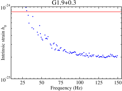
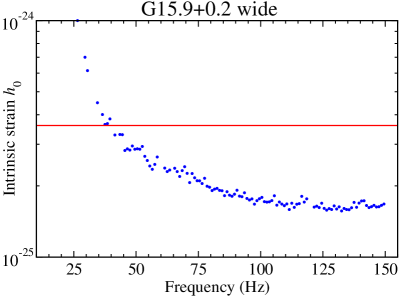
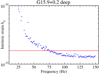
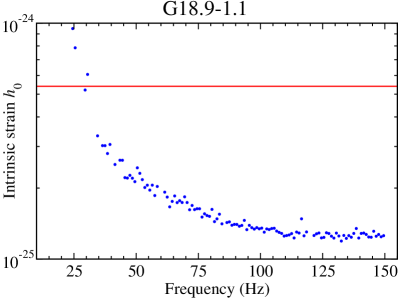
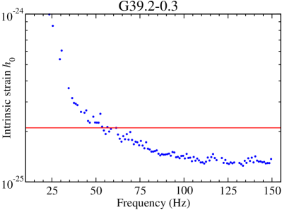
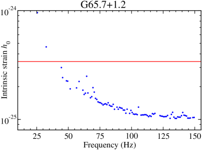
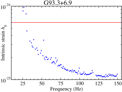
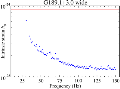
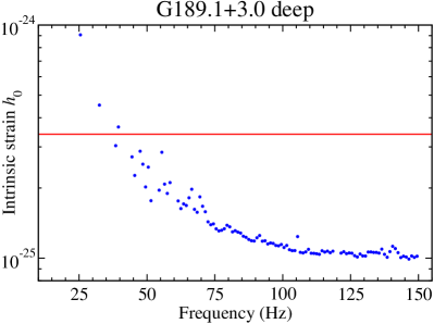
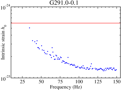
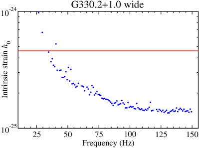
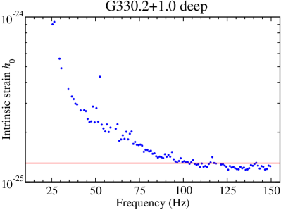
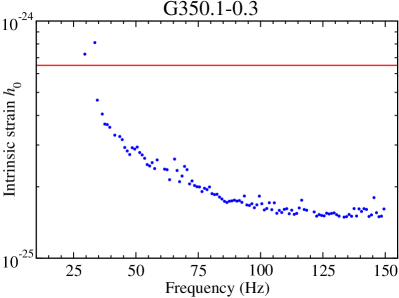
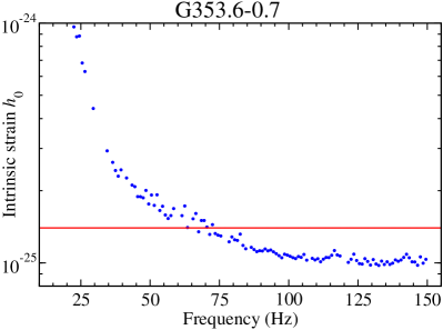
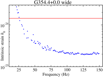
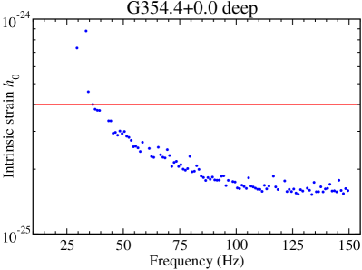
The upper limits on which survived the veto check are plotted as a function of frequency in Figs. 1–4. Generally older targets produced better upper limits because longer integration times were possible for the fixed computational cost per target. The data files, including points not visible on the plots, are included in the supplemental material to this article EPA . In terms of the “sensitivity depth” defined in Ref. Dreissigacker et al. (2018), these searches ranged from about 45 Hz-1/2 for young SNRs to 70 Hz-1/2 for older SNRs.
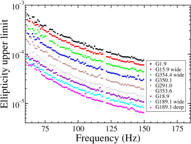
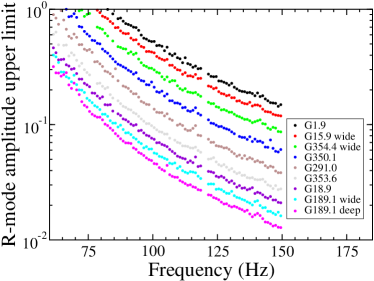
Upper limits on can be converted to upper limits on neutron star ellipticity using e.g. Wette et al. (2008)
| (5) |
and to upper limits on a particular measure of -mode amplitude Lindblom et al. (1998) using Owen (2010)
| (6) |
The numerical values are uncertain by a factor of roughly two or three due to uncertainties in the unknown neutron star mass and equation of state.
We plot upper limits on for a selection of searches representing the range of these limits in the left panel of Fig. 5 and on in the right panel. The differences between curves are primarily due to to differences in the distances to the sources.
IV Discussion
Although we detected no signals, we placed the best upper limits yet on GW amplitude from these twelve SNRs. Our upper limits are as good (low) as and were generally about a factor of two better than similar limits on the same SNRs using O1 data from Ref. Abbott et al. (2019a). Our upper limits are also (for several targets) up to a factor of two better than all-sky limits on O2 data from Ref. Abbott et al. (2019d). For SNR G1.9+0.3 our limits were about the same as Ref. Abbott et al. (2019d) in our frequency band, but we covered five times the range of Also, our searches included which is rare in the literature. Our searches included two new parameter sets for two of the SNRs. Part of the improved sensitivity over comparable O1 searches Abbott et al. (2019a) was due to the reduced noise of O2 and part was due to our longer searches at lower frequencies, which seem to be characteristic of known young pulsars. Because of our focus on lower frequencies, our upper limits on neutron-star ellipticity and -mode amplitude are less impressive than those from searches which extended to higher frequencies Abbott et al. (2019a). Our limits on -mode amplitude do not reach the level expected by the most detailed exploration of nonlinear saturation mechanisms Bondarescu et al. (2009). But our ellipticity limits still in some cases approach a few times the rough maximum currently expected from normal neutron stars Johnson-McDaniel and Owen (2013); Baiko and Chugunov (2018).
We are working on code to more efficiently handle high frequencies and long spin-down ages. With these improvements and ever improving strain noise from Advanced LIGO, the prospects for continuous GW detection will improve.
Acknowledgements.
This research has made use of data, software and/or web tools obtained from the Gravitational Wave Open Science Center (https://www.gw-openscience.org), a service of LIGO Laboratory, the LIGO Scientific Collaboration and the Virgo Collaboration. LIGO is funded by the U.S. National Science Foundation. Virgo is funded by the French Centre National de Recherche Scientifique (CNRS), the Italian Istituto Nazionale della Fisica Nucleare (INFN) and the Dutch Nikhef, with contributions by Polish and Hungarian institutes. This research was supported in part by NSF grants PHY-1604244, DMS-1620366, and PHY-1912419 to the University of California at San Diego; and by PHY-1912625 to Texas Tech University. The authors acknowledge computational resources provided by the High Performance Computing Center (HPCC) of Texas Tech University at Lubbock (http://www.depts.ttu.edu/hpcc/).References
- Glampedakis and Gualtieri (2018) K. Glampedakis and L. Gualtieri, Gravitational waves from single neutron stars: an advanced detector era survey, Astrophys. Space Sci. Libr. 457, 673 (2018), arXiv:1709.07049 [astro-ph.HE] .
- Wette et al. (2008) K. Wette et al. (LIGO Scientific), Searching for gravitational waves from Cassiopeia A with LIGO, Proceedings, 18th International Conference on General Relativity and Gravitation (GRG18) and 7th Edoardo Amaldi Conference on Gravitational Waves (Amaldi7), Sydney, Australia, July 2007, Class. Quant. Grav. 25, 235011 (2008), arXiv:0802.3332 [gr-qc] .
- Abadie et al. (2010) J. Abadie et al., First search for gravitational waves from the youngest known neutron star, Astrophys. J. 722, 1504 (2010).
- Abadie et al. (2011) J. Abadie, B. P. Abbott, R. Abbott, M. Abernathy, T. Accadia, F. Acernese, C. Adams, R. Adhikari, P. Ajith, B. Allen, and et al., Directional Limits on Persistent Gravitational Waves Using LIGO S5 Science Data, Physical Review Letters 107, 271102 (2011), arXiv:1109.1809 [astro-ph.CO] .
- Aasi et al. (2015) J. Aasi, B. P. Abbott, R. Abbott, T. Abbott, M. R. Abernathy, F. Acernese, K. Ackley, C. Adams, T. Adams, P. Addesso, and et al., Searches for Continuous Gravitational Waves from Nine Young Supernova Remnants, Astrophys. J. 813, 39 (2015), arXiv:1412.5942 [astro-ph.HE] .
- Sun et al. (2016) L. Sun, A. Melatos, P. D. Lasky, C. T. Y. Chung, and N. S. Darman, Cross-correlation search for continuous gravitational waves from a compact object in SNR 1987A in LIGO Science run 5, Phys. Rev. D 94, 082004 (2016), arXiv:1610.00059 [gr-qc] .
- Zhu et al. (2016) S. J. Zhu, M. A. Papa, H.-B. Eggenstein, R. Prix, K. Wette, B. Allen, O. Bock, D. Keitel, B. Krishnan, B. Machenschalk, M. Shaltev, and X. Siemens, Einstein@Home search for continuous gravitational waves from Cassiopeia A, Phys. Rev. D 94, 082008 (2016), arXiv:1608.07589 [gr-qc] .
- Abbott et al. (2017a) B. P. Abbott, R. Abbott, T. D. Abbott, M. R. Abernathy, F. Acernese, K. Ackley, C. Adams, T. Adams, P. Addesso, R. X. Adhikari, and et al., Directional Limits on Persistent Gravitational Waves from Advanced LIGO’s First Observing Run, Physical Review Letters 118, 121102 (2017a), arXiv:1612.02030 [gr-qc] .
- Abbott et al. (2019a) B. P. Abbott et al. (LIGO Scientific, Virgo), Searches for Continuous Gravitational Waves from 15 Supernova Remnants and Fomalhaut b with Advanced LIGO, Astrophys. J. 875, 122 (2019a), arXiv:1812.11656 [astro-ph.HE] .
- Ming et al. (2019) J. Ming et al., Results from an Einstein@Home search for continuous gravitational waves from Cassiopeia A, Vela Jr. and G347.3, Phys. Rev. D100, 024063 (2019), arXiv:1903.09119 [gr-qc] .
- Abbott et al. (2019b) B. P. Abbott et al. (LIGO Scientific, Virgo), Directional limits on persistent gravitational waves using data from Advanced LIGO’s first two observing runs, Phys. Rev. D100, 062001 (2019b), arXiv:1903.08844 [gr-qc] .
- Aasi et al. (2013) J. Aasi, J. Abadie, B. P. Abbott, T. Abbott, R. an d Abbott, M. R. Abernathy, T. Accadia, F. Acernese, C. Adams, T. Adams, and et al., Directed search for continuous gravitational waves from the Galactic center, Phys. Rev. D 88, 102002 (2013), arXiv:1309.6221 [gr-qc] .
- Piccinni et al. (2019) O. J. Piccinni, P. Astone, S. D’Antonio, S. Frasca, G. Intini, I. La Rosa, P. Leaci, S. Mastrogiovanni, A. Miller, and C. Palomba, A directed Search for Continuous Gravitational-Wave Signals from the Galactic Center in Advanced LIGO Second Observing Run, (2019), arXiv:1910.05097 [gr-qc] .
- Abbott et al. (2017b) B. P. Abbott, R. Abbott, T. D. Abbott, M. R. Abernathy, F. Acernese, K. Ackley, C. Adams, T. Adams, P. Addesso, R. X. Adhikari, and et al., Search for continuous gravitational waves from neutron stars in globular cluster NGC 6544, Phys. Rev. D 95, 082005 (2017b), arXiv:1607.02216 [gr-qc] .
- Manchester et al. (2005) R. N. Manchester, G. B. Hobbs, A. Teoh, and M. Hobbs, The Australia Telescope National Facility pulsar catalogue, Astron. J. 129, 1993 (2005), arXiv:astro-ph/0412641 [astro-ph] .
- Reich et al. (1984) W. Reich, E. Fuerst, C. G. T. Haslam, P. Steffen, and K. Reif, A radio continuum survey of the Galactic Plane at 11 CM wavelength. I - The area L = 357.4 to 76 deg, B = -1.5 to +1.5 deg, Astron. Astrophys. Suppl. 58, 197 (1984).
- Reynolds et al. (2008) S. P. Reynolds, K. J. Borkowski, D. A. Green, U. Hwang, I. Harrus, and R. Petre, The Youngest Galactic Supernova Remnant: G1.9+0.3, Astrophys. J. Lett. 680, L41 (2008), arXiv:0803.1487 .
- Reynolds et al. (2006) S. P. Reynolds, K. J. Borkowski, U. Hwang, I. Harrus, R. Petre, and G. Dubner, A New Young Galactic Supernova Remnant Containing a Compact Object: G15.9+0.2, Astrophys. J. Lett. 652, L45 (2006), astro-ph/0610323 .
- Tüllmann et al. (2010) R. Tüllmann, P. P. Plucinsky, T. J. Gaetz, P. Slane, J. P. Hughes, I. Harrus, and T. G. Pannuti, Searching for the Pulsar in G18.95-1.1: Discovery of an X-ray Point Source and Associated Synchrotron Nebula with Chandra, Astrophys. J. 720, 848 (2010).
- Harrus et al. (2004) I. M. Harrus, P. O. Slane, J. P. Hughes, and P. P. Plucinsky, An X-Ray Study of the Supernova Remnant G18.95-1.1, Astrophys. J. 603, 152 (2004), arXiv:astro-ph/0311410 .
- Olbert et al. (2003) C. M. Olbert, J. W. Keohane, K. A. Arnaud, K. K. Dyer, S. P. Reynolds, and S. Safi-Harb, Chandra Detection of a Pulsar Wind Nebula Associated with Supernova Remnant 3C 396, Astrophys. J. Lett. 592, L45 (2003).
- Su et al. (2011) Y. Su, Y. Chen, J. Yang, B.-C. Koo, X. Zhou, D.-R. Lu, I.-G. Jeong, and T. DeLaney, Molecular Environment and Thermal X-ray Spectroscopy of the Semicircular Young Composite Supernova Remnant 3C 396, Astrophys. J. 727, 43 (2011), arXiv:1011.2330 [astro-ph.GA] .
- Arzoumanian et al. (2008) Z. Arzoumanian, S. Safi-Harb, T. L. Landecker, R. Kothes, and F. Camilo, Chandra Confirmation of a Pulsar Wind Nebula in DA 495, Astrophys. J. 687, 505 (2008), arXiv:0806.3766 .
- Kothes et al. (2004) R. Kothes, T. L. Landecker, and M. Wolleben, H I Absorption of Polarized Emission: A New Technique for Determining Kinematic Distances to Galactic Supernova Remnants, Astrophys. J. 607, 855 (2004).
- Kothes et al. (2008) R. Kothes, T. L. Landecker, W. Reich, S. Safi-Harb, and Z. Arzoumanian, DA 495: An Aging Pulsar Wind Nebula, Astrophys. J. 687, 516 (2008), arXiv:0807.0811 .
- Jiang et al. (2007) B. Jiang, Y. Chen, and Q. D. Wang, The Chandra View of DA 530: A Subenergetic Supernova Remnant with a Pulsar Wind Nebula?, Astrophys. J. 670, 1142 (2007), arXiv:0708.0953 .
- Foster and Routledge (2003) T. Foster and D. Routledge, A New Distance Technique for Galactic Plane Objects, Astrophys. J. 598, 1005 (2003).
- Olbert et al. (2001) C. M. Olbert, C. R. Clearfield, N. E. Williams, J. W. Keohane, and D. A. Frail, A Bow Shock Nebula around a Compact X-Ray Source in the Supernova Remnant IC 443, Astrophys. J. Lett. 554, L205 (2001), arXiv:astro-ph/0103268 .
- Fesen and Kirshner (1980) R. A. Fesen and R. P. Kirshner, Spectrophotometry of the supernova remnant IC 443, Astrophys. J. 242, 1023 (1980).
- Petre et al. (1988) R. Petre, A. E. Szymkowiak, F. D. Seward, and R. Willingale, A comprehensive study of the X-ray structure and spectrum of IC 443, Astrophys. J. 335, 215 (1988).
- Swartz et al. (2015) D. A. Swartz, G. G. Pavlov, T. Clarke, G. Castelletti, V. E. Zavlin, N. Bucciantini, M. Karovska, A. J. van der Horst, M. Yukita, and M. C. Weisskopf, High Spatial Resolution X-Ray Spectroscopy of the IC 443 Pulsar Wind Nebula and Environs, Astrophys. J. 808, 84 (2015), arXiv:1506.05507 [astro-ph.HE] .
- Slane et al. (2012) P. Slane, J. P. Hughes, T. Temim, R. Rousseau, D. Castro, D. Foight, B. M. Gaensler, S. Funk, M. Lemoine-Goumard, J. D. Gelfand, D. A. Moffett, R. G. Dodson, and J. P. Bernstein, A Broadband Study of the Emission from the Composite Supernova Remnant MSH 11-62, Astrophys. J. 749, 131 (2012), arXiv:1202.3371 [astro-ph.HE] .
- Moffett et al. (2001) D. Moffett, B. Gaensler, and A. Green, G291.0-0.1: Powered by a pulsar?, in Young Supernova Remnants: Eleventh Astrophysics Conference, AIP Conf. Proc., Vol. 565, edited by S. S. Holt and U. Hwang (Melville, NY: AIP, 2001) pp. 333–336.
- Park et al. (2006) S. Park, K. Mori, O. Kargaltsev, P. O. Slane, J. P. Hughes, D. N. Burrows, G. P. Garmire, and G. G. Pavlov, Discovery of a Candidate Central Compact Object in the Galactic Nonthermal SNR G330.2+1.0, Astrophys. J. 653, L37 (2006), arXiv:astro-ph/0610004 .
- McClure-Griffiths et al. (2001) N. M. McClure-Griffiths, A. J. Green, J. M. Dickey, B. M. Gaensler, R. F. Haynes, and M. H. Wieringa, The Southern Galactic Plane Survey: The Test Region, Astrophys. J. 551, 394 (2001), arXiv:astro-ph/0012302 .
- Park et al. (2009) S. Park, O. Kargaltsev, G. G. Pavlov, K. Mori, P. O. Slane, J. P. Hughes, D. N. Burrows, and G. P. Garmire, Nonthermal X-Rays from Supernova Remnant G330.2+1.0 and the Characteristics of its Central Compact Object, Astrophys. J. 695, 431 (2009), arXiv:0809.4281 .
- Torii et al. (2006) K. Torii, H. Uchida, K. Hasuike, H. Tsunemi, Y. Yamaguchi, and S. Shibata, Discovery of a Featureless X-Ray Spectrum in the Supernova Remnant Shell of G330.2+1.0, Pub. Astron. Soc. Japan 58, L11 (2006), arXiv:astro-ph/0601569 .
- Gaensler et al. (2008) B. M. Gaensler, A. Tanna, P. O. Slane, C. L. Brogan, J. D. Gelfand, N. M. McClure-Griffiths, F. Camilo, C. Ng, and J. M. Miller, The (Re-)Discovery of G350.1-0.3: A Young, Luminous Supernova Remnant and Its Neutron Star, Astrophys. J. Lett. 680, L37 (2008), arXiv:0804.0462 .
- Lovchinsky et al. (2011) I. Lovchinsky, P. Slane, B. M. Gaensler, J. P. Hughes, C.-Y. Ng, J. S. Lazendic, J. D. Gelfand, and C. L. Brogan, A Chandra Observation of Supernova Remnant G350.1-0.3 and Its Central Compact Object, Astrophys. J. 731, 70 (2011), arXiv:1102.5333 [astro-ph.HE] .
- Halpern and Gotthelf (2010) J. P. Halpern and E. V. Gotthelf, Two Magnetar Candidates in HESS Supernova Remnants, Astrophys. J. 710, 941 (2010), arXiv:0912.4985 [astro-ph.HE] .
- Tian et al. (2008) W. W. Tian, D. A. Leahy, M. Haverkorn, and B. Jiang, Discovery of the Radio and X-Ray Counterpart of TeV -Ray Source HESS J1731-347, Astrophys. J. Lett. 679, L85 (2008), arXiv:0801.3254 .
- Roy and Pal (2013) S. Roy and S. Pal, Discovery of the small-diameter, young supernova remnant g354.4+0.0, The Astrophysical Journal 774, 150 (2013).
- Jaranowski et al. (1998) P. Jaranowski, A. Krolak, and B. F. Schutz, Data analysis of gravitational - wave signals from spinning neutron stars. 1. The Signal and its detection, Phys. Rev. D58, 063001 (1998), arXiv:gr-qc/9804014 [gr-qc] .
- Cutler and Schutz (2005) C. Cutler and B. F. Schutz, The Generalized F-statistic: Multiple detectors and multiple GW pulsars, Phys. Rev. D72, 063006 (2005), arXiv:gr-qc/0504011 [gr-qc] .
- Vallisneri et al. (2015) M. Vallisneri, J. Kanner, R. Williams, A. Weinstein, and B. Stephens, The LIGO Open Science Center, Proceedings, 10th International LISA Symposium: Gainesville, Florida, USA, May 18-23, 2014, J. Phys. Conf. Ser. 610, 012021 (2015), arXiv:1410.4839 [gr-qc] .
- Abbott et al. (2019c) R. Abbott et al. (LIGO Scientific, Virgo), Open data from the first and second observing runs of Advanced LIGO and Advanced Virgo, (2019c), arXiv:1912.11716 [gr-qc] .
- Cahillane et al. (2018) M. Cahillane, M. Hulko, J. S. Kissel, et al., LIGO-G1800319, Tech. Rep. (2018) https://dcc.ligo.org/LIGO-G1800319/public.
- Green (2019) D. A. Green, A revised catalogue of 294 Galactic supernova remnants, Journal of Astrophysics and Astronomy 40, 36 (2019), arXiv:1907.02638 [astro-ph.GA] .
- Hurley-Walker et al. (2019) N. Hurley-Walker et al., Candidate radio supernova remnants observed by the GLEAM survey over and , Publ. Astron. Soc. Austral. 36, e048 (2019), arXiv:1911.08124 [astro-ph.HE] .
- LIGO Scientific Collaboration (2018) LIGO Scientific Collaboration, LIGO Algorithm Library - LALSuite, free software (GPL) (2018).
- Covas et al. (2018) P. B. Covas, A. Effler, E. Goetz, P. M. Meyers, A. Neunzert, M. Oliver, B. L. Pearlstone, V. J. Roma, R. M. S. Schofield, V. B. Adya, and et al., Identification and mitigation of narrow spectral artifacts that degrade searches for persistent gravitational waves in the first two observing runs of Advanced LIGO, Phys. Rev. D 97, 082002 (2018), arXiv:1801.07204 [astro-ph.IM] .
- Abbott et al. (2019d) B. P. Abbott et al. (LIGO Scientific, Virgo), All-sky search for continuous gravitational waves from isolated neutron stars using Advanced LIGO O2 data, Phys. Rev. D100, 024004 (2019d), arXiv:1903.01901 [astro-ph.HE] .
- (53) PRD will insert URL here.
- Dreissigacker et al. (2018) C. Dreissigacker, R. Prix, and K. Wette, Fast and Accurate Sensitivity Estimation for Continuous-Gravitational-Wave Searches, Phys. Rev. D98, 084058 (2018), arXiv:1808.02459 [gr-qc] .
- Lindblom et al. (1998) L. Lindblom, B. J. Owen, and S. M. Morsink, Gravitational radiation instability in hot young neutron stars, Phys. Rev. Lett. 80, 4843 (1998), arXiv:gr-qc/9803053 [gr-qc] .
- Owen (2010) B. J. Owen, How to adapt broad-band gravitational-wave searches for r-modes, Phys. Rev. D82, 104002 (2010), arXiv:1006.1994 [gr-qc] .
- Bondarescu et al. (2009) R. Bondarescu, S. A. Teukolsky, and I. Wasserman, Spinning down newborn neutron stars: Nonlinear development of the r-mode instability, Phys. Rev. D 79, 104003 (2009), arXiv:0809.3448 .
- Johnson-McDaniel and Owen (2013) N. K. Johnson-McDaniel and B. J. Owen, Maximum elastic deformations of relativistic stars, Phys. Rev. D 88, 044004 (2013), arXiv:1208.5227 [astro-ph.SR] .
- Baiko and Chugunov (2018) D. A. Baiko and A. I. Chugunov, Breaking properties of neutron star crust, Mon. Not. Roy. Astron. Soc. 480, 5511 (2018), arXiv:1808.06415 [astro-ph.HE] .