A Time Domain Approach for the Exponential Stability of a Nondissipative Linearized Compressible Flow-Structure PDE System

Abstract

This work is motivated by a longstanding interest in the long time behavior of flow-structure interaction (FSI) PDE dynamics. Such coupled PDE systems are ubiquitous in modeling of various natural phenomena, and in particular have many applications in fluid dynamics, aeroelasticity and gas dynamics. We consider a linearized compressible flow structure interaction (FSI) PDE model with a view of analyzing the stability properties of both the compressible flow and plate solution components. In our earlier work, we gave an answer in the affirmative to question of uniform stability for finite energy solutions of said compressible flow-structure system, by means of a “frequency domain” approach. However, the frequency domain method of proof in that work is not “robust” (insofar as we can see), when one wishes to study longtime behavior of solutions of compressible flow-structure PDE models which track the appearance of the ambient state onto the boundary interface (i.e., $\kappa=1$ in flow PDE component (2)). Nor is a frequency domain approach in this earlier work availing when one wishes to consider the dynamics, in long time, of solutions to physically relevant nonlinear versions of the compressible flow-structure PDE system under present consideration (e.g., the Navier-Stokes nonlinearity in the PDE flow component, or a nonlinearity of Berger/Von Karman type in the plate equation). Accordingly, in the present work, we operate in the time domain by way of obtaining the necessary energy estimates which culminate in an alternative proof for the uniform stability of finite energy compressible flow-structure solutions. This novel time domain proof will be used in our forthcoming paper which addresses the existence of compact global attractors for the corresponding nonlinear coupled system in which the material derivative – which incorporates the aforesaid ambient state – of the interaction surface will be taken into account. Since there is a need to avoid steady states in our stability analysis, as a prerequisite result, we also show here that zero is an eigenvalue for the generators of flow-structure systems, whether the material derivative term be absent or present. Moreover, we provide a clean characterization of the (one dimensional) zero eigenspace, with or without material derivative, under an appropriate assumption on the underlying ambient vector field.

Key terms: Flow-structure interaction, compressible flows, uniform stability

1
Introduction

The linearized compressible flow-structure PDE model which we will consider arises in the context of the design of various engineering systems and the study of gas dynamics. This coupled system describes the interaction between a plate and a given compressible gas flow. In contrast to incompressible fluid flows, wherein the fluid density is assumed to be a constant, compressible gas flow models will contain an additional fluid density variable, and involve other state spaces. For further details the reader is referred to [14, 7, 8, 4].

The presence of the density (pressure) equations in compressible cases will tend to make the analysis quite different than that for incompressible flows; in particular, one must deal with the extra density (pressure) solution variable. Moreover, and intrinsic to the problem under consideration, linearization of the compressible Navier Stokes equation occurs around a rest state that contains an arbitrary ambient vector field $\mathbf{U}$. Qualitative properties of this model – i.e., wellposedness and long term analysis in the sense of global attractors (in the presence of the von Karman plate nonlinearity) were firstly analyzed in [14], in the case $\mathbf{U}=0.$ However, the case $\mathbf{U}\neq 0$ was recognized to be challenging, since the presence of a nonzero ambient field introduces problematic terms such as $\mathbf{U}\cdot\nabla p,$ (where $p$ is the pressure variable), a term which is “unbounded” with respect to the underlying finite energy space of wellposedness.

With respect to compressible flow-structure PDE systems with underlying nonzero ambient terms: A positive answer to the wellposedness question was given in [7] in the case $\mathbf{U}\neq 0$; exponential stability of finite energy solutions to this model was shown in [4], again in the case $\mathbf{U}\neq 0$. With a view of handling the aforesaid troublesome term $\mathbf{U}\cdot\nabla p$, a frequency domain approach is invoked in [4]. By way of appropriately estimating $\mathbf{U}\cdot\nabla p$ in [4], as a static (and not time dependent term), the frequency domain approaches allows for an appropriate decomposition of static Stokes flow, and an eventual invocation of the nonsmooth domain version of the Agmon-Douglis-Nirenberg Theorem; see p. 75 of [19]. In addition to dealing with unbounded term $\mathbf{U}\cdot\nabla p$, a large part of the work in [4] is devoted to a spectral analysis of the compressible flow-structure generator, by way of ultimately invoking the wellknown resolvent criteria for exponential decay in [26] and [37].

Although the methodology set forth in [4] is effective in establishing exponential stability for solutions of the compressible flow-structure PDE model (2)-(4) below, with $\kappa=0$, it’s use seems limited when dealing with (2)-(4) when the physically relevant material derivative term is present (i.e., $\kappa=1$; see [8] for the modeling aspects of this problem; also [24]). In particular, since the presence of the material derivative term $\mathbf{U}\cdot\nabla w$ on the boundary interface constitutes an unbounded perturbation of the compressible flow-structure PDE system, a necessary spectral analysis for $\kappa=1$, analogous to that in [4], is problematic. In addition, the critical frequency domain estimates which were obtained in [4] for the linear problem do not lend themselves readily to adaptation so as to handle nonlinear versions of (2)-(4), versions in which the Navier-Stokes or von Karman plate nonlinearities are present. Consequently, the problem of analyzing long time behavior for nonlinear compressible flow-structure PDE systems – particularly in the sense of global attractors – must be undertaken in the ”time domain” rather than the ”frequency domain”.

Accordingly, the principal contribution of the present manuscript is to give an alternative proof for the exponential stability of the solutions via a certain multiplier method in the time domain. In particular, our main (gradient type) multiplier is based upon the solution of a certain Neumann problem, a solution which is sufficiently smooth, even considering the unavoidable boundary interface singularities; see [20] and [28]. We should also note that the application of this multiplier is practicable and convenient, due to the characterization (compatibility condition) of the stabilizable finite energy space $[Null(\mathcal{A})]^{\bot}$ where $\mathcal{A}$ is the semigroup generator of the system.

As we said, besides being of intrinsic interest in its own right, this manuscript will also serve as a blue print for our forthcoming work which will address the existence of compact attractors for nonlinear flow-structure PDE interactions, in which the material derivative appears in the normal component boundary condition of the compressible flow variable (i.e., $\kappa=1$). This material derivative term on the boundary interface represents an unbounded perturbation of the compressible flow-structure semigroup generator, in addition to the presence of a nonlocal nonlinearity (von Karman or Berger). With this future work in mind, in this manuscript, we also analyze the Null space of the generator of the system, in the presence or absence of the material derivative on the interaction surface $\Omega$. Again, our main reason for doing this is to avoid finite energy initial data which gives rise to steady states. In the course of proof, which partly involves a necessary assumption on the ambient field $\mathbf{U}$, we show that, despite the unboundedness presented by the material derivative perturbation, the Null Space of the “material derivative” generator $\mathcal{A}_{1}$, $(\kappa=1)$ will coincide with Null Space of the “material derivative free” generator $\mathcal{A}_{0}$, $(\kappa=0).$

In what follows we provide the PDE description of the interaction model under the study. Let the flow domain $\mathcal{O}$ be a bounded subset of $\mathbb{R}^{3}$, with boundary $\partial\mathcal{O}$. Moreover, $\partial\mathcal{O}=\overline{S}\cup\overline{\Omega}$, with $S\cap\Omega=\emptyset$, and with (structure) domain $\Omega\subset\mathbb{R}^{3}$ being a flat portion of $\partial\mathcal{O}$. In particular, assume that $\partial\mathcal{O}$ has the following specific configuration:

$$\Omega\subset\left\{x=(x_{1,}x_{2},0)\right\}\,\text{\ and \ surface }S\subset\left\{x=(x_{1,}x_{2},x_{3}):x_{3}\leq 0\right\}\,.$$ (1)

and $\ \mathbf{n}(\mathbf{x})$ denotes the unit outward normal vector to $\partial\mathcal{O}$ where $\left.\mathbf{n}\right|_{\Omega}=[0,0,1]$. We also impose additional following geometrical conditions on $\mathcal{O}:$

Condition 1

The flow domain $\mathcal{O}$ should be a curvilinear polyhedral domain –i.e., $\mathcal{O}$ has a finite set of smooth  edges and corners; see, [22] – which satisfies the following assumptions:

1. Each corner of the boundary $\partial\mathcal{O}$ -if any- is diffeomorphic to a convex cone,

2. Each point on an edge of the boundary $\partial\mathcal{O}$ is diffeomorphic to a wedge with opening $<\pi.$

Remark 2

The point of making such assumptions on the geometry of domain $\mathcal{O}$ is that they will allow for our application of elliptic results for solutions of second order boundary value problems on corner domains; see [20]. In particular, these results will be invoked in our time dependent multiplier method by way of proving our uniform stability result.

The usual, familiar geometries can be considered as in Figure 1.

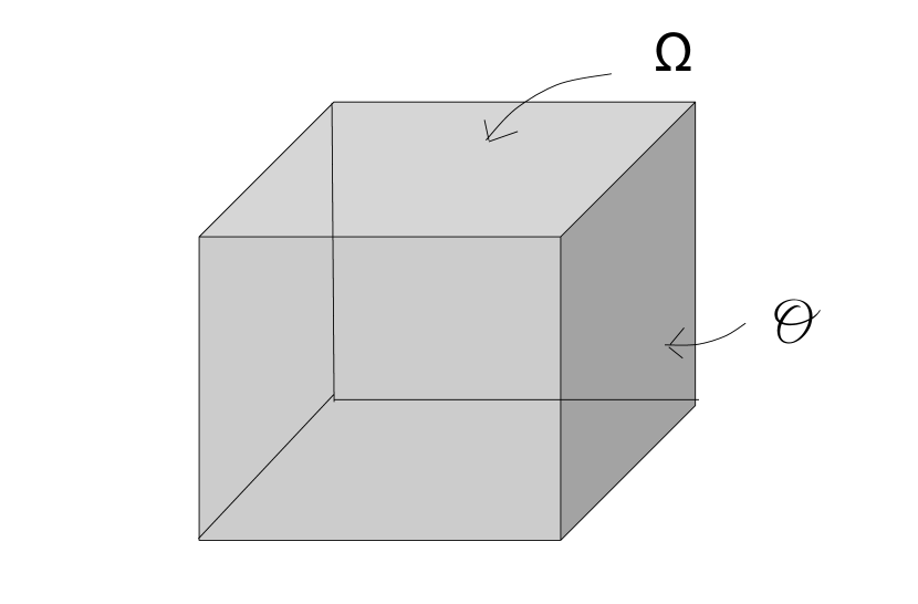
Figure 1: Polyhedral Flow-Structure Geometries

The coupled PDE system which we will consider is the result of a linearization which is undertaken in [14] and [7]: Within the three-dimensional geometry $\mathcal{O}$, the compressible Navier-Stokes equations are present, assuming the flow which they describe to be barotropic. This system is linearized with respect to some reference rest state of the form $\left\{p_{\ast},\mathbf{U},\varrho_{\ast}\right\}$: the pressure and density components ${p_{\ast},\varrho_{\ast}}$ are scalars, and the arbitrary ambient field $\mathbf{U}:\mathcal{O}\rightarrow\mathbb{R}^{3}$

$$\mathbf{U}(x_{1},x_{2},x_{3})=[U_{1}(x_{1},x_{2},x_{3}),U_{2}(x_{1},x_{2},x_{3}),U_{3}(x_{1},x_{2},x_{3})]$$

is given.

In [14] and [7], we already see that non-critical lower order terms are deleted, and the aforesaid pressure and density reference constants are set equal to unity. Thus, we are presented with the following system of equations, in solution variables $\mathbf{u}(x_{1},x_{2},x_{3},t)$ (flow velocity), $p(x_{1},x_{2},x_{3},t)$ (pressure), $w(x_{1},x_{2},t)$ (elastic plate displacement) and $w_{t}(x_{1},x_{2},t)$ (elastic plate velocity):

$$\left\{\begin{array}[]{l}p_{t}+\mathbf{U}\cdot\nabla p+div~{}\mathbf{u}=0~{}\text{ in }~{}\mathcal{O}\times(0,\infty)\\ \mathbf{u}_{t}+\mathbf{U}\cdot\nabla\mathbf{u}-div~{}\sigma(\mathbf{u})+\eta\mathbf{u}+\nabla p=0~{}\text{ in }~{}\mathcal{O}\times(0,\infty)\\ (\sigma(\mathbf{u})\mathbf{n}-p\mathbf{n})\cdot\boldsymbol{\tau}=0~{}\text{ on }~{}\partial\mathcal{O}\times(0,\infty)\\ \mathbf{u}\cdot\mathbf{n}=0~{}\text{ on }~{}S\times(0,\infty)\\ \mathbf{u}\cdot\mathbf{n}=w_{t}+\kappa\mathbf{U}\cdot\nabla w\text{ \ \ on }~{}\Omega\times(0,\infty)\text{ (where }\kappa=0\text{ or }\kappa=1\text{)}\end{array}\right.$$ (7)

$$\left\{\begin{array}[]{l}w_{tt}+\Delta^{2}w+\left[2\nu\partial_{x_{3}}(\mathbf{u})_{3}+\lambda\text{div}(\mathbf{u})-p\right]_{\Omega}=0~{}\text{ on }~{}\Omega\times(0,\infty)\\ w=\frac{\partial w}{\partial\nu}=0~{}\text{ on }~{}\partial\Omega\times(0,\infty)\end{array}\right.$$ (10)

$$\begin{array}[]{c}\left[p(0),\mathbf{u}(0),w(0),w_{t}(0)\right]=\left[p_{0},\mathbf{u}_{0},w_{0},w_{1}\right]\end{array}$$ (12)

(where above, $\nabla w=\left[w_{x_{1}},w_{x_{2}},0\right]$; see [8]). We note that the flow linearization is taken with respect to some generally inhomogeneous compressible Navier-Stokes system; thus, $\mathbf{U}$ need not be divergence free generally; there are also initially forcing terms in the pressure and flow equations (and energy level terms) which we have neglected, since they do not effect the current analysis. This flow-structure system is a generalization of that considered by the late Igor Chueshov in [14] with therein fixed vector field $\mathbf{U}=\mathbf{0}$. In contrast, the PDE system (7)-(12) depends upon a generally non-zero, fixed, ambient vector field $\mathbf{U}$ about which the linearization takes place. The quantity $\eta>0$ represents a drag force of the domain on the viscous flow. In addition, the quantity $\mathbf{\tau}$ in (7) is in the space $TH^{1/2}(\partial\mathcal{O)}$ of tangential vector fields of Sobolev index 1/2; that is,

$$\mathbf{\tau}\in TH^{1/2}(\partial\mathcal{O)=}\{\mathbf{v}\in\mathbf{H}^{\frac{1}{2}}(\partial\mathcal{O})~{}:~{}\left.\mathbf{v}\right|_{\partial\mathcal{O}}\cdot\mathbf{n}=0~{}\text{ on }~{}\partial\mathcal{O}\}.$$ (13)

(See e.g., p.846 of [12].) In addition, we take ambient field $\mathbf{U}$ to be in the space

$$\mathbf{V}_{0}=\{\mathbf{v}\in\mathbf{H}^{1}(\mathcal{O})~{}:~{}\left.\mathbf{v}\right|_{\partial\mathcal{O}}\cdot\mathbf{n}=0~{}\text{ on }~{}\partial\mathcal{O}\}$$ (14)

(This vanishing of the boundary for ambient fields is a standard assumption in compressible flow literature; see [18],[41],[29],[2].)

Moreover, the stress and strain tensors in the flow PDE component of (7)-(12) are defined respectively as

$$\sigma(\mathbf{\mu})=2\nu\epsilon(\mathbf{\mu})+\lambda[I_{3}\cdot\epsilon(\mathbf{\mu})]I_{3};\text{ \ }\epsilon_{ij}(\mathbf{\mu})=\dfrac{1}{2}\left(\frac{\partial\mathbf{\mu}_{j}}{\partial x_{i}}+\frac{\partial\mathbf{\mu}_{i}}{\partial x_{j}}\right)\text{, \ }1\leq i,j\leq 3,$$

where Lamé Coefficients $\lambda\geq 0$ and $\nu>0$. The associated finite energy space will be

$$\mathcal{H}\equiv L^{2}(\mathcal{O})\times\mathbf{L}^{2}(\mathcal{O})\times H_{0}^{2}(\Omega)\times L^{2}(\Omega)$$ (15)

which is a Hilbert space, topologized by the following standard inner product:

$$(\mathbf{y}_{1},\mathbf{y}_{2})_{\mathcal{H}}=(p_{1},p_{2})_{L^{2}(\mathcal{O})}+(\mathbf{u}_{1},\mathbf{u}_{2})_{\mathbf{L}^{2}(\mathcal{O})}+(\Delta w_{1},\Delta w_{2})_{L^{2}(\Omega)}+(v_{1},v_{2})_{L^{2}(\Omega)}$$ (16)

for any $\mathbf{y}_{i}=(p_{i},\mathbf{u}_{i},w_{i},v_{i})\in\mathcal{H},~{}i=1,2.$

Remark 3

As we noted in [7], the flow PDE boundary conditions which are in (7) are the so-called impermeability-slip conditions [11, 13]: namely, no flow passes through the boundary – in particular, the normal component of the flow field $\mathbf{u}$ on the active boundary portion $\Omega$ matches the plate velocity $w_{t}$ – and on $\partial\mathcal{O}$ there is no stress in the tangential direction $\tau$.

2 Functional Setting of the Problem

Throughout, for a given domain $D$, the norm of corresponding space $L^{2}(D)$ will be denoted as $||\cdot||_{D}$ (or simply $||\cdot||$ when the context is clear). Inner products in $L^{2}(\mathcal{O})$ or $\mathbf{L}^{2}(\mathcal{O})$ will be denoted by $(\cdot,\cdot)_{\mathcal{O}}$, whereas inner products $L^{2}(\partial\mathcal{O})$ will be written as $\langle\cdot,\cdot\rangle_{\partial\mathcal{O}}$. We will also denote pertinent duality pairings as $\left\langle\cdot,\cdot\right\rangle_{X\times X^{\prime}}$ for a given Hilbert space $X$. The space $H^{s}(D)$ will denote the Sobolev space of order $s$, defined on a domain $D$; $H_{0}^{s}(D)$ will denote the closure of $C_{0}^{\infty}(D)$ in the $H^{s}(D)$-norm $\|\cdot\|_{H^{s}(D)}$. We make use of the standard notation for the boundary trace of functions defined on $\mathcal{O}$, which are sufficently smooth: i.e., for a scalar function $\phi\in H^{s}(\mathcal{O})$, $\frac{1}{2}<s<\frac{3}{2}$, $\gamma(\phi)=\phi\big{|}_{\partial\mathcal{O}},$ which is a well-defined and surjective mapping on this range of $s$, owing to the Sobolev Trace Theorem on Lipschitz domains (see e.g., [34], or Theorem 3.38 of [33]).

With respect to the above setting, the PDE system given in (7)-(12) can be written as an ODE in Hilbert space $\mathcal{H}.$ That is, if $\Phi(t)=\left[p,\mathbf{u},w,w_{t}\right]\in C([0,T];\mathcal{H})$ solves the problem (7)-(12), then, for the respective cases $\kappa=0$ or $\kappa=1$ there is a modeling operator $\mathcal{A_{\kappa}}:D(\mathcal{A_{\kappa}})\subset\mathcal{H}\rightarrow\mathcal{H}$ such that $\Phi(\cdot)$ satisfies

$$\dfrac{d}{dt}\Phi(t) = \mathcal{A}_{\kappa}\Phi(t);$$

$$\Phi(0) = \Phi_{0}$$ (17)

Here $\mathcal{A}_{\kappa}:D(\mathcal{A}_{\kappa})\subset\mathcal{H}\rightarrow\mathcal{H}$ is defined as follows:

$$\mathcal{A}_{\kappa}=\left[\begin{array}[]{cccc}-\mathbf{U}\mathbb{\cdot}\nabla(\cdot)&-\text{div}(\cdot)&0&0\\ -\mathbb{\nabla(\cdot)}&\text{div}\sigma(\cdot)-\eta I-\mathbf{U}\mathbb{\cdot\nabla(\cdot)}&0&0\\ 0&0&0&I\\ \left.\left[\cdot\right]\right|_{\Omega}&-\left[2\nu\partial_{x_{3}}(\cdot)_{3}+\lambda\text{div}(\cdot)\right]_{\Omega}&-\Delta^{2}&0\end{array}\right];$$ (18)

$$D(\mathcal{A}_{\kappa})=\{(p_{0},\mathbf{u}_{0},w_{1},w_{2})\in L^{2}(\mathcal{O})\times\mathbf{H}^{1}(\mathcal{O})\times H_{0}^{2}(\Omega)\times H_{0}^{2}(\Omega)~{}:~{}\text{properties }(A.i)\text{--}(A.v)~{}~{}\text{hold}\},$$

where

1. $\mathbf{U}\cdot\nabla p_{0}\in L^{2}(\mathcal{O}).$

2. $\text{div}~{}\sigma(\mathbf{u}_{0})-\nabla p_{0}\in\mathbf{L}^{2}(\mathcal{O})$. (Consequently, we infer the boundary trace regularity
   $\left[\sigma(\mathbf{u}_{0})\mathbf{n}-p_{0}\mathbf{n}\right]_{\partial\mathcal{O}}\in\mathbf{H}^{-\frac{1}{2}}(\partial\mathcal{O})$.)

3. $-\Delta^{2}w_{1}-\left[2\nu\partial_{x_{3}}(\mathbf{u}_{0})_{3}+\lambda\text{div}(\mathbf{u}_{0})\right]_{\Omega}+\left.p_{0}\right|_{\Omega}\in L^{2}(\Omega).$

4. $\left(\sigma(\mathbf{u}_{0})\mathbf{n}-p_{0}\mathbf{n}\right)\bot~{}TH^{1/2}(\partial\mathcal{O})$. That is,

   $$\left\langle\sigma(\mathbf{u}_{0})\mathbf{n}-p_{0}\mathbf{n},\mathbf{\tau}\right\rangle_{\mathbf{H}^{-\frac{1}{2}}(\partial\mathcal{O})\times\mathbf{H}^{\frac{1}{2}}(\partial\mathcal{O})}=0\text{ \ for every }\mathbf{\tau}\in TH^{1/2}(\partial\mathcal{O})$$

   (and so $\left(\sigma(\mathbf{u}_{0})\mathbf{n}-p_{0}\mathbf{n}\right)\cdot\mathbf{\tau}=0$ in the sense of distributions; see Remark 3.1 of [7]).

5. The flow velocity component $\mathbf{u}_{0}=\mathbf{f}_{0}+\widetilde{\mathbf{f}}_{0}$, where $\mathbf{f}_{0}\in\mathbf{V}_{0}$ and $\widetilde{\mathbf{f}}_{0}\in\mathbf{H}^{1}(\mathcal{O})$ satisfies

   $$\left.\widetilde{\mathbf{f}}_{0}\right|_{\partial\mathcal{O}}=\begin{cases}0&~{}\text{ on }~{}S\\ \left(w_{2}+\kappa\mathbf{U}\cdot\nabla w_{1}\right)\mathbf{n}&~{}\text{ on}~{}\Omega\end{cases}$$

   (and so $\left.\mathbf{f}_{0}\right|_{\partial\mathcal{O}}\in TH^{1/2}(\partial\mathcal{O})$).

In [7] and [8], it was shown that solutions to the compressible flow-structure PDE system (7)-(12), again for $\kappa=0$ or $\kappa=1$, with initial data in said finite energy space $\mathcal{H}$, can be associated with a strongly continuous semigroup $\left\{e^{\mathcal{A}_{\kappa}t}\right\}\,_{t\geq 0}\subset\mathcal{L}(\mathcal{H)}$ which yields the following wellposedness result:

Theorem 4

(See Theorem 3.1 of [7] and Theorem 5.1 of [8].) Assume that ambient vector field $\mathbf{U}\in\mathbf{V}_{0}\cap\mathbf{H}^{3}(\mathcal{O})$ (when $k=0$ and $k=1.$) Additionally, in the case $k=1,$ let $\mathbf{U}|_{\Omega}\in C^{2}(\bar{\Omega}).$

(i) (Wellposedness) The flow-structure operator $\mathcal{A}_{\kappa}:D(\mathcal{A}_{\kappa})\subset\mathcal{H}\rightarrow\mathcal{H}$, generates a $C_{0}$-semigroup on $\mathcal{H}$. Accordingly, the solution of (7)-(12) – with initial data $[p_{0},\mathbf{u}_{0},w_{0},w_{1}]\in$ $\mathcal{H}$ – may be given by

$$\begin{bmatrix}p(t)\\ \mathbf{u}(t)\\ w(t)\\ w_{t}(t)\end{bmatrix}=e^{\mathcal{A}_{\kappa}t}\begin{bmatrix}p_{0}\\ \mathbf{u}_{0}\\ w_{0}\\ w_{1}\end{bmatrix}\in C[(0,\infty);\mathcal{H}].$$ (19)

(ii) (Energy relation) We define

$$E(t)=\frac{1}{2}\left[\left\|p(t)\right\|_{\mathcal{O}}^{2}+\left\|\mathbf{u}(t)\right\|_{\mathcal{O}}^{2}+\left\|\Delta w(t)\right\|_{{\Omega}}^{2}+\left\|w_{t}(t)\right\|_{{\Omega}}^{2}\right],$$ (20)

where $\left[p(t),\mathbf{u}(t),\Delta w(t),w_{t}(t)\right]$ is the solution of compressible flow-structure system (7)-(12), given explicitly by (19). Then for all $0\leq s<t$, we have the relation

$$E(t)+\int\limits_{s}^{t}\left[(\sigma(\mathbf{u(}\tau\mathbf{)}),\epsilon(\mathbf{u(}\tau\mathbf{))}_{\mathcal{O}}+\eta\left\|\mathbf{u(}\tau\mathbf{)}\right\|_{\mathcal{O}}^{2}\right]d\tau=E(s)+\frac{1}{2}\int\limits_{s}^{t}\int\limits_{\mathcal{O}}{div}(\mathbf{U})\left[\left|p(\tau)\right|^{2}+\left|\mathbf{u(}\tau\mathbf{)}\right|^{2}\right]d\mathcal{O}d\tau$$

$$+\kappa\int_{s}^{t}\left\langle\left[2\nu\partial_{x_{3}}(\mathbf{u})_{3}+\lambda\text{div}(\mathbf{u})-p\right]_{\Omega},\mathbf{U}\cdot\nabla w\right\rangle_{\Omega}d\tau.$$ (21)

From the expression (21), it is seen that the generator $\mathcal{A}_{\kappa}:D(\mathcal{A}_{\kappa})\subset\mathcal{H}\rightarrow\mathcal{H}$ does not dissipate the energy of the system (7)-(12). None the less, in [4], we establish that solutions of (7)-(12) decay uniformly, with respect to intial data which is $\mathcal{H}$-orthogonal to the one dimensional null space of $\mathcal{A}_{0}$ (see Theorem 2 (ii) therein).

The main intent of the present work is to (i) discern the null space for $\mathcal{A}_{1}:D(\mathcal{A}_{1})\subset\mathcal{H}\rightarrow\mathcal{H}$, under appropriate assumptions, and (ii) give an alternative proof of uniform stability for the (material derivative-free) semigroup $\left\{e^{\mathcal{A}_{0}t}\right\}_{t\geq 0}\subset\mathcal{L}(\mathcal{H})$, which in contrast to the frequency domain approach of [4], is based on the invocation of appropriate multipliers in the time domain.

3 The Null Space of $\mathcal{A}_{\kappa}:D(\mathcal{A}_{\kappa})\subset\mathcal{H}\rightarrow\mathcal{H}$

In the process of analyzing the long term dynamics of the system (7)-(12), we need to avoid steady states so as to reasonably consider the possibility of finite energy solutions tending to the zero state at infinity. In fact, in the case $k=0$, the fact that zero is an eigenvalue for the generator $\mathcal{A}_{0}$ was proved in [4]. Also an explicit characterization for the corresponding zero eigenspace was given there, again in the case $k=0.$ However, in the presence of the unbounded –material derivative– term $\mathbf{U}\cdot\nabla w$ it is not at all clear a priori that the case $\kappa=1$ should give rise to the same zero eigenspace. In this section, we give a positive answer to this question: indeed, zero is also an eigenvalue for the generator $\mathcal{A}_{1}$ whose null space is identical with that for $\mathcal{A}_{0}.$ (As we said, this spectral information will be needed in our future work on longtime behavior properties of nonlinear compressible flow-structure PDE dynamics, with material derivative term in place.) Before giving this result let us recall the following lemma (see Lemma 10 of [4]):

Lemma 5

Let $\mathbf{U}\in\mathbf{V}_{0}\cap\mathbf{H}^{3}(\mathcal{O})$ and $\left\|{div}(\mathbf{U})\right\|_{\infty}\leq\mathfrak{C}_{0}^{\ast}(\Psi)$ (sufficiently small), where $\mathfrak{C}_{0}^{\ast}(\Psi)$ is a positive constant with $\Psi=\Psi\left(\mathbf{U}\right)\equiv\left[\left\|\mathbf{U}\right\|_{\mathbf{H}^{3}(\mathcal{O})}+1\right]$. Then one has the following:

The subspace $Null(\mathcal{A}_{0}\mathcal{)}\subset\mathcal{H}$ of the flow-structure generator $\mathcal{A}_{0}:D(\mathcal{A}_{0})\subset\mathcal{H}\rightarrow\mathcal{H}$ is one dimensional. In particular, $Null(\mathcal{A}_{0}\mathcal{)}$ is given explicity as

$$Null(\mathcal{A}_{0}\mathcal{)}=Span\left\{\left[\begin{array}[]{c}1\\ 0\\ {{\mathring{A}}^{-1}(1)}\\ 0\end{array}\right]\right\},$$ (22)

where $\mathring{A}:L^{2}(\Omega)\rightarrow L^{2}(\Omega)$ is the elliptic operator

$$\mathring{A}\varpi=\Delta^{2}\varpi\text{, with }D(\mathring{A})=\{w\in H_{0}^{2}(\Omega):\Delta^{2}w\in L^{2}(\Omega)\}.\text{\ \ }$$ (23)

Now, we give the same result for the generator $\mathcal{A}_{1}$ but we note that if we wish for the generator $\mathcal{A}_{1}:D(\mathcal{A}_{1})\subset\mathcal{H}\rightarrow\mathcal{H}$ of the flow-structure PDE system to have the same one dimensional null space in (22), as for $\mathcal{A}_{0}$, despite the additional (unbounded) material derivative term, then: from the domain criterion (A.v) and (22), one must necessarily have, for $\kappa=1$, the relation

$$\mathbf{U}\cdot\nabla{{\mathring{A}}^{-1}(1)=0}\text{ on }\Omega$$ (24)

where the biharmonic operator $\mathring{A}$ is as in (23). That is,

$$\left[U_{1}(x_{1},x_{2},0),U_{2}(x_{1},x_{2},0\right]\cdot\left[\frac{\partial}{\partial x_{1}}{{\mathring{A}}^{-1}(1),}\frac{\partial}{\partial x_{2}}{{\mathring{A}}^{-1}(1)}\right]=0.$$

Lemma 6

(a) Suppose that the ambient field $\mathbf{U}$ satisfies (24), and moreover $\left\{\left\|{div}(\mathbf{U})\right\|_{\infty},\left\|\left.\mathbf{U}\right|_{\Omega}\right\|_{\boldsymbol{H}^{\frac{1}{2}}(\Omega)\cap\mathbf{L}^{\infty}(\Omega)}\right\}\leq\mathfrak{C}_{0}^{\ast}(\Psi)$ (sufficiently small), where $\mathfrak{C}_{0}^{\ast}(\Psi)$ is a positive constant with $\Psi=\Psi\left(\mathbf{U}\right)\equiv\left[\left\|\mathbf{U}\right\|_{\mathbf{H}^{3}(\mathcal{O})}+1\right]$. Then, as in Lemma 5, the subspace $Null(\mathcal{A}_{1}\mathcal{)}\subset\mathcal{H}$ of the (when the material derivative is taken into account) flow-structure generator $\mathcal{A}_{1}$ is given by

$$Null(\mathcal{A}_{1})\mathcal{=}Null(\mathcal{A}_{0}\mathcal{)}=Span\left\{\left[\begin{array}[]{c}1\\ 0\\ {{\mathring{A}}^{-1}(1)}\\ 0\end{array}\right]\right\}$$ (25)

(b) The orthogonal complement of $Null(\mathcal{A}_{\kappa}\mathcal{)}$ ($\kappa=0$ or $\kappa=1$) admits of the characterization

$$[Null(\mathcal{A}_{\kappa}\mathcal{)}]^{\bot}=\mathcal{\{}[p_{0},\mathbf{u}_{0},w_{1},w_{2}]\in\mathcal{H}:\int\limits_{\mathcal{O}}p_{0}d\mathcal{O}+\int\limits_{\Omega}w_{1}d\Omega=0\mathcal{\}}.$$ (26)

Proof of Lemmas 5 and 6

 We focus here on the touchier case $\kappa=1$, inasmuch as the details for $\kappa=0$ are subsumed in the material derivative case. (See also [4].)

Suppose $\Phi=[p_{0},\mathbf{u}_{0},w_{1},w_{2}]\in D(\mathcal{A}_{1})$ is a solution of

$$\mathcal{A}_{1}\Phi=\mathbf{0}\text{,}$$ (27)

where $\mathcal{A}_{1}:D(\mathcal{A}_{1})\subset\mathcal{H}\rightarrow\mathcal{H}$ is as given in (18). (Without loss of generality, we take $\Phi$ to be real-valued.) With respect to the pressure component, we invoke the $L^{2}$-decomposition

$$p_{0}=q_{0}+c_{0}\text{,}$$ (28)

where

$$q_{0}\text{ satisfies }\int\limits_{\mathcal{O}}q_{0}d\mathcal{O}=0\text{, \ and \ }c_{0}=\text{constant.}$$ (29)

Therewith, in PDE terms, the abstract relation then becomes

$$\left\{\begin{array}[]{l}-\mathbf{U}\cdot\nabla q_{0}-div~{}\mathbf{u}_{0}=0\text{ \ in }~{}\mathcal{O}\\ -\nabla q_{0}+div~{}\sigma(\mathbf{u}_{0})-\eta\mathbf{u}_{0}-\mathbf{U}\cdot\nabla\mathbf{u}_{0}=0~{}\text{ \ in }~{}\mathcal{O}\\ w_{2}=0\text{ \ on }~{}\Omega\\ -\Delta^{2}w_{1}-\left[2\nu\partial_{x_{3}}(\mathbf{u}_{0})_{3}+\lambda\text{div}(\mathbf{u}_{0})-p_{0}\right]_{\Omega}=0~{}\text{ on }~{}\Omega\end{array}\right.$$ (34)

$$\left\{\begin{array}[]{l}(\sigma(\mathbf{u}_{0})\mathbf{n}-p_{0}\mathbf{n})\cdot\boldsymbol{\tau}=0\text{ \ on }~{}\partial\mathcal{O}\\ \mathbf{u}_{0}\cdot\mathbf{n}=0~{}\text{ on }~{}S\\ \mathbf{u}_{0}\cdot\mathbf{n}=\mathbf{U}\cdot\nabla w_{1}~{}\text{ on }~{}\Omega\\ w_{1}=\frac{\partial w_{1}}{\partial\nu}=0~{}\text{ on }~{}\partial\Omega.\end{array}\right.$$ (39)

We have immediately then,

$$w_{2}=0\text{.}$$ (40)

Secondly, we multiply the pressure PDE component in (34)-(39) by $p_{0}$ and the fluid PDE component by $\mathbf{u}_{0}$. Subsequent integrations and integrations by parts, and a consideration of domain criteria (A.iv), (A.v) (and (40)), yield then

$$\begin{array}[]{l}\left(\sigma(\mathbf{u}_{0}),\epsilon(\mathbf{u}_{0})\right)_{\mathcal{O}}+\eta\left\|\mathbf{u}_{0}\right\|_{\mathcal{O}}^{2}=\frac{1}{2}\left({div}(\mathbf{U})p_{0},p_{0}\right)_{\mathcal{O}}+\frac{1}{2}\left({div}(\mathbf{U})\mathbf{u}_{0},\mathbf{u}_{0}\right)_{\mathcal{O}}\\ \text{ \ \ \ }\ -\left\langle c_{0},\mathbf{U}\cdot\nabla w_{1}\right\rangle_{\Omega}+\left\langle\left[2\nu\partial_{x_{3}}(\mathbf{u}_{0})_{3}+\lambda\text{div}(\mathbf{u}_{0})-q_{0}\right]_{\Omega},u_{3}\right\rangle_{\Omega}\end{array}$$ (41)

(For the last term on RHS, we are also using the fact that $\mathbf{n}=[0,0,1]$ on $\Omega$.) Therewith, combining the decomposition (28) with Green’s formula and the fact that $\mathbf{U}\in\mathbf{V}_{0}$, we then obtain

$$\left(\sigma(\mathbf{u}_{0}),\epsilon(\mathbf{u}_{0})\right)_{\mathcal{O}}+\eta\left\|\mathbf{u}_{0}\right\|_{\mathcal{O}}^{2}=\left({div}(\mathbf{U})c_{0},q_{0}\right)_{\mathcal{O}}$$

$$\text{ \ }-\left\langle c_{0},\mathbf{U}\cdot\nabla w_{1}\right\rangle_{\Omega}+\left\langle\left[2\nu\partial_{x_{3}}(\mathbf{u}_{0})_{3}+\lambda\text{div}(\mathbf{u}_{0})-q_{0}\right]_{\Omega},u_{3}\right\rangle_{\Omega}$$

$$\text{ \ }+\frac{1}{2}\left({div}(\mathbf{U})q_{0},q_{0}\right)_{\mathcal{O}}+\frac{1}{2}\left({div}(\mathbf{U})\mathbf{u}_{0},\mathbf{u}_{0}\right)_{\mathcal{O}}.$$ (42)

To estimate the first term on right hand side of (42), we multiply the pressure equation in (34) by constant component $c_{0}$ of (28) and integrate over $\mathcal{O}$. This gives,

$$-\left(\mathbf{U}\cdot\nabla q_{0},c_{0}\right)=\left({div}\mathbf{u}_{0},c_{0}\right).$$

Subsequently we integrate by parts both sides of this relation, while bearing in mind the domain criterion (A.v) and (40) (and the fact that $\mathbf{U}\in\mathbf{V}_{0}$), so as to have

$$\left({{div}}(\mathbf{U})q_{0},c_{0}\right)_{\mathcal{O}}=\left\langle c_{0},\mathbf{U}\cdot\nabla w_{1}\right\rangle_{\Omega}.$$

Applying this relation to (42) gives now

$$\left(\sigma(\mathbf{u}_{0}),\epsilon(\mathbf{u}_{0})\right)_{\mathcal{O}}+\eta\left\|\mathbf{u}_{0}\right\|_{\mathcal{O}}^{2} = \left\langle\left[2\nu\partial_{x_{3}}(\mathbf{u}_{0})_{3}+\lambda\text{div}(\mathbf{u}_{0})-q_{0}\right]_{\Omega},u_{3}\right\rangle_{\Omega}$$

$$+\frac{1}{2}\left({div}(\mathbf{U})q_{0},q_{0}\right)_{\mathcal{O}}+\frac{1}{2}\left({div}(\mathbf{U})\mathbf{u}_{0},\mathbf{u}_{0}\right)_{\mathcal{O}};$$

and subsequently invoking the domain criterion (A.v) (for $\kappa=1$) and the mechanical equation on $\Omega$, we have now

$$\left(\sigma(\mathbf{u}_{0}),\epsilon(\mathbf{u}_{0})\right)_{\mathcal{O}}+\eta\left\|\mathbf{u}_{0}\right\|_{\mathcal{O}}^{2} = \left\langle\left[2\nu\partial_{x_{3}}(\mathbf{u}_{0})_{3}+\lambda\text{div}(\mathbf{u}_{0})-q_{0}\right]_{\Omega},\mathbf{U}\cdot\nabla\left({{\mathring{A}}^{-1}(c}_{0}-\left[2\nu\partial_{x_{3}}(\mathbf{u}_{0})_{3}+\lambda\text{div}(\mathbf{u}_{0})-q_{0}\right]_{\Omega}{)}\right)\right\rangle_{\Omega}$$

$$+\frac{1}{2}\left({div}(\mathbf{U})q_{0},q_{0}\right)_{\mathcal{O}}+\frac{1}{2}\left({div}(\mathbf{U})\mathbf{u}_{0},\mathbf{u}_{0}\right)_{\mathcal{O}};$$

and subsequently invoking (24) yields then

$$\left(\sigma(\mathbf{u}_{0}),\epsilon(\mathbf{u}_{0})\right)_{\mathcal{O}}+\eta\left\|\mathbf{u}_{0}\right\|_{\mathcal{O}}^{2} = -\left\langle\left[2\nu\partial_{x_{3}}(\mathbf{u}_{0})_{3}+\lambda\text{div}(\mathbf{u}_{0})-q_{0}\right]_{\Omega},\mathbf{U}\cdot\nabla\left({{\mathring{A}}^{-1}}\left[2\nu\partial_{x_{3}}(\mathbf{u}_{0})_{3}+\lambda\text{div}(\mathbf{u}_{0})-q_{0}\right]_{\Omega}\right)\right\rangle_{\Omega}$$ (43)

$$+\frac{1}{2}\left({div}(\mathbf{U})q_{0},q_{0}\right)_{\mathcal{O}}+\frac{1}{2}\left({div}(\mathbf{U})\mathbf{u}_{0},\mathbf{u}_{0}\right)_{\mathcal{O}}.$$

To make use of this relation, we appeal to the estimate provided by Theorem 2.4 or Remark 2.5 of [40], for solution pair $\left(\mathbf{u}_{0},q_{0}\right)$ of (Stokes system) (34). Namely, we have

$$\left\|q_{0}\right\|_{\mathcal{O}}^{2}+\left(\sigma(\mathbf{u}_{0}),\epsilon(\mathbf{u}_{0})\right)_{\mathcal{O}}+\eta\left\|\mathbf{u}_{0}\right\|_{\mathcal{O}}^{2}$$

$$\leq C\left(\left\|\mathbf{U}\cdot\nabla\mathbf{u}_{0}\right\|_{\mathcal{O}}^{2}+\left\|{div}(\mathbf{u}_{0})\right\|_{\mathcal{O}}^{2}+\left\|\mathbf{u}_{0}\right\|_{\mathbf{H}^{\frac{1}{2}}(\partial\mathcal{O})}^{2}\right)$$

(We are also implicitly using Korn’s Inequality.) Estimating right hand side by Korn’s Inequality and the Sobolev Trace Theorem gives now

$$\left\|q_{0}\right\|_{\mathcal{O}}^{2}+\left(\sigma(\mathbf{u}_{0}),\epsilon(\mathbf{u}_{0})\right)_{\mathcal{O}}+\eta\left\|\mathbf{u}_{0}\right\|_{\mathcal{O}}^{2}$$ (44)

$$\leq \mathfrak{C}_{1}\Psi(\mathbf{U})\left[\left(\sigma(\mathbf{u}_{0}),\epsilon(\mathbf{u}_{0})\right)_{\mathcal{O}}+\eta\left\|\mathbf{u}_{0}\right\|_{\mathcal{O}}^{2}\right],$$

where the term $\Psi(\mathbf{U})$ is as given in the statement of Lemma 6, and positive constant $\mathfrak{C}_{1}$ is independent of $\mathbf{U}.$ (We are implicitly using here the Sobolev Imbedding Theorem with respect to field $\mathbf{U}\in\mathbf{H}^{3}(\mathcal{O})$). Applying (44) to the right hand side of (43) gives then,

$$\left(\sigma(\mathbf{u}_{0}),\epsilon(\mathbf{u}_{0})\right)_{\mathcal{O}}+\eta\left\|\mathbf{u}_{0}\right\|_{\mathcal{O}}^{2}\leq$$

$$\left|\left\langle\left[2\nu\partial_{x_{3}}(\mathbf{u}_{0})_{3}+\lambda\text{div}(\mathbf{u}_{0})-q_{0}\right]_{\Omega},\mathbf{U}\cdot\nabla\left({{\mathring{A}}^{-1}}\left[2\nu\partial_{x_{3}}(\mathbf{u}_{0})_{3}+\lambda\text{div}(\mathbf{u}_{0})-q_{0}\right]_{\Omega}\right)\right\rangle_{\Omega}\right|$$

$$+{\mathfrak{C}_{2}(\Psi(\mathbf{U}))}\left\|{div}(\mathbf{U})\right\|_{\infty}\left[\left(\sigma(\mathbf{u}_{0}),\epsilon(\mathbf{u}_{0})\right)_{\mathcal{O}}+\eta\left\|\mathbf{u}_{0}\right\|_{\mathcal{O}}^{2}\right],$$

whence we obtain

$$\left(\sigma(\mathbf{u}_{0}),\epsilon(\mathbf{u}_{0})\right)_{\mathcal{O}}+\eta\left\|\mathbf{u}_{0}\right\|_{\mathcal{O}}^{2}$$ (45)

$$\leq C\left\|\left.\mathbf{U}\right|_{\Omega}\right\|_{\boldsymbol{H}^{\frac{1}{2}}(\Omega)\cap\mathbf{L}^{\infty}(\Omega)}\left\|\left[2\nu\partial_{x_{3}}(\mathbf{u}_{0})_{3}+\lambda\text{div}(\mathbf{u}_{0})-q_{0}\right]_{\Omega}\right\|_{H^{-\frac{1}{2}}(\Omega)}^{2}$$

$$+{\mathfrak{C}_{2}(\Psi(\mathbf{U}))}\left\|{div}(\mathbf{U})\right\|_{\infty}\left[\left(\sigma(\mathbf{u}_{0}),\epsilon(\mathbf{u}_{0})\right)_{\mathcal{O}}+\eta\left\|\mathbf{u}_{0}\right\|_{\mathcal{O}}^{2}\right].$$

In turn, an integration by parts, the estimates (44), and (45) (and a rescaling of parameter $\epsilon>0$) give

$$\left\|\sigma(\mathbf{u}_{0})\cdot\mathbf{n}-q_{0}\mathbf{n}\right\|_{\mathbf{H}^{-\frac{1}{2}}(\partial\mathcal{O})}^{2}\leq C\left(\left\|q_{0}\right\|_{\mathcal{O}}^{2}+\left(\sigma(\mathbf{u}_{0}),\epsilon(\mathbf{u}_{0})\right)_{\mathcal{O}}+\eta\left\|\mathbf{u}_{0}\right\|_{\mathcal{O}}^{2}+\left\|\mathbf{U}\cdot\nabla\mathbf{u}_{0}\right\|_{\mathcal{O}}^{2}\right).$$ (46)

Combining (45) and (46) gives now

$$\left\|\sigma(\mathbf{u}_{0})\cdot\mathbf{n}-q_{0}\mathbf{n}\right\|_{\mathbf{H}^{-\frac{1}{2}}(\partial\mathcal{O})}^{2}+\left(\sigma(\mathbf{u}_{0}),\epsilon(\mathbf{u}_{0})\right)_{\mathcal{O}}+\eta\left\|\mathbf{u}_{0}\right\|_{\mathcal{O}}^{2}$$ (47)

$$\leq {\mathfrak{C}_{3}(\Psi(\mathbf{U}))}\left(\left\|\left.\mathbf{U}\right|_{\Omega}\right\|_{\boldsymbol{H}^{\frac{1}{2}}(\Omega)\cap\mathbf{L}^{\infty}(\Omega)}\left\|\left[2\nu\partial_{x_{3}}(\mathbf{u}_{0})_{3}+\lambda\text{div}(\mathbf{u}_{0})-q_{0}\right]_{\Omega}\right\|_{H^{-\frac{1}{2}}(\Omega)}^{2}\right.$$

$$\left.+\left\|{div}(\mathbf{U})\right\|_{\infty}\left[\left(\sigma(\mathbf{u}_{0}),\epsilon(\mathbf{u}_{0})\right)_{\mathcal{O}}+\eta\left\|\mathbf{u}_{0}\right\|_{\mathcal{O}}^{2}\right]\right).$$

If we now specify

$$\max\left\{\left\|{div}(\mathbf{U})\right\|_{\infty},\left\|\left.\mathbf{U}\right|_{\Omega}\right\|_{\boldsymbol{H}^{\frac{1}{2}}(\Omega)\cap\mathbf{L}^{\infty}(\Omega)}\right\}<\frac{1}{{\mathfrak{C}_{3}(\Psi(\mathbf{U}))}}\equiv{\mathfrak{C}_{0}^{\ast}(\Psi(\mathbf{U}));}$$ (48)

where again $\Psi\left(\mathbf{U}\right)\equiv\left[\left\|\mathbf{U}\right\|_{\mathbf{H}^{3}(\mathcal{O})}+1\right]$, we then deduce that

$$\mathbf{u}_{0}=\mathbf{0}\text{ and }q_{0}=0\text{.}$$ (49)

(We are also implicitly using Korn’s Inequality). Consequently, via (28) we obtain

$$p_{0}=c_{0}\text{, where }c_{0}\text{ is constant.}$$ (50)

Returning to the mechanical equation on $\Omega$ in (34), we then have

$$w_{1}={{\mathring{A}}^{-1}(c_{0}),}$$ (51)

where again $\mathring{A}^{-1}:L^{2}(\Omega)\rightarrow L^{2}(\Omega)$ is the operator defined in (23). The relations (40), (49), (50) and (51) give the conclusion of (a) of Lemma 6 for $\kappa=1$. Given the definition of the $\mathcal{H}$-inner product as well as the definition in (23) of $\mathring{A}:L^{2}(\Omega)\rightarrow L^{2}(\Omega)$, the relation in (b) of Lemma 6 is immediate.    $\square$

Remark 7

Suppose the curvilinear polyhedron $\mathcal{O}$ is strictly an “edge domain” – i.e., the geometry has no corners – such that each point on an edge of $\partial\mathcal{O}$ is diffeomorphic to a wedge with opening $<\pi/2$. Then an example of an ambient field $\mathbf{U\in V}_{0}\cap\mathbf{H}^{3}(\mathcal{O})$ which meets the compatibility condition (24) can be constructed as follows: Let boundary data $\mathbf{g}$ satisfy

$$\mathbf{g}=\left\{\begin{array}[]{l}\left[\begin{array}[]{c}-\frac{\partial}{\partial x_{2}}{{\mathring{A}}^{-1}(1)}\\ \frac{\partial}{\partial x_{1}}{{\mathring{A}}^{-1}(1)}\\ 0\end{array}\right]\in\mathbf{H}^{s}(\Omega)\text{ \ on }\Omega\\ \\ \mathbf{0}\text{ \ on }\partial\mathcal{O}.\end{array}\right.$$

Therewith, $\mathbf{g}\in\mathbf{H}^{3}(\partial\mathcal{O})$; see e.g., Theorem 3.33, p. 95, of [33]. Here, we are implicitly using the fact that $\left.\frac{\partial}{\partial x_{i}}{{\mathring{A}}^{-1}(1)}\right|_{\partial\Omega}=0$. Subsequently, we can invoke the well-established elliptic regularity results on edge domains – see; e.g., [22] – for Neumann problem, with boundary data $\mathbf{g}$, so as to secure a $\mathbf{U}$ which meets the requirements of Lemma 6, after an appropriate scaling.

4 Exponential Stability – A Time Domain Approach

This section is devoted to giving an alternative proof for the exponential stability of the solutions to material derivative-free system (7)-(12) (i.e., the case $k=0$.) Unlike the frequency domain approach followed in [4] to obtain this stability result, we give the proof of Theorem (8) in time domain, an approach which involves a gradient type multiplier by way of obtaining necessary energy estimates. As we mentioned before, the alternative proof which we provide here can in principle be used in any long term analysis for corresponding nonlinear systems. In fact, the time domain approach which we develop here will be our key departure point in the forthcoming paper related to compact global attractors of the system (7)-(12), in the presence of the material derivative, as well as given structural (von Karman) nonlinearity.

With the notation adopted above, we give the following exponential decay result for all initial data taken from $[Null(\mathcal{A)}]^{\bot}$, which is a one dimensional subspace of $\mathcal{H}$ (see Lemma 6(b)):

Theorem 8

Let the ambient vector field $\mathbf{U}\in\mathbf{V}_{0}\cap\mathbf{H}^{3}(\mathcal{O})$ and the geometrical assumptions in Condition 1 hold. Additionally, assume that $\left\|{div}(\mathbf{U})\right\|_{\infty}$ is sufficiently small. Then the (material derivative -free) $C_{0}$-semigroup $\left\{\left.e^{\mathcal{A}_{0}t}\right|_{[Null(\mathcal{A}_{0}\mathcal{)}]^{\bot}}\right\}_{t\geq 0}\in\mathcal{L}\left([Null(\mathcal{A}_{0}\mathcal{)}]^{\bot}\right)$ decays exponentially. In particular, there exist constants $\mathfrak{M}>0$ and $\omega>0$ such that the solution to the flow-structure PDE system (7)-(12), with initial data $\Phi_{0}=\left[p_{0},\mathbf{u}_{0},w_{0}w_{1}\right]\in[Null(\mathcal{A}_{0}\mathcal{)}]^{\bot}$, obeys the uniform decay rate

$$\left\|e^{\mathcal{A}_{0}t}\Phi_{0}\right\|_{\mathcal{H}}\leq\mathfrak{M}e^{-\omega t}\left\|\Phi_{0}\right\|_{\mathcal{H}}\text{, \ for all }t>0\text{.}$$ (52)

Remark 9

In our time domain approach, the geometrical assumptions on the polyhedral flow domain $\mathcal{O}$ are necessary, since in the course of proof of Theorem 8, we appeal to higher regularity results for the Neumann problem on domains with corners (see [28] and [22] for further details.) They are analogous to the geometrical assumptions made in [4], in which the frequency domain approach requires the invocation of higher regularity results for static Stokes flow on corner domains; see [19].

Remark 10

We note that for $\kappa=0$, one has the invariance of $\mathcal{A}_{0}$ and its associated $C_{0}$-semigroup $\left\{e^{\mathcal{A}_{0}t}\right\}_{t\geq 0}$ on $[Null(\mathcal{A}_{0}\mathcal{)}]^{\bot}$; in particular, $\left\{\left.e^{\mathcal{A}_{0}t}\right|_{[Null(\mathcal{A)}]^{\bot}}\right\}\subset\mathcal{L}\left([Null(\mathcal{A}_{0}\mathcal{)}]^{\bot}\right)$, for $\kappa=0.$ (See Proposition 13 of [4].)

Proof of Theorem 8.

The proof is based on the application of a multiplier which is intrinsic to the compressible flow-structure PDE system under consideration. In order to deal with the lack of $H^{1}$-regularity of the pressure variable $p$ – which is partly manifested in the unbounded term $\mathbf{U}\cdot\nabla p$ – this special multiplier exploits the compatibility condition given in (26) for any data of $[Null(\mathcal{A}_{0}\mathcal{)}]^{\bot}$ so as to ultimately enable us to obtain the necessary observability estimate for the energy of the system.

We will consider the following system (in the case $\kappa=0$ in (7)-(12) ) and initial data $\Phi(0)=\left[p(0),\mathbf{u}(0),w(0),w_{t}(0)\right]=\left[p_{0},\mathbf{u}_{0},w_{0},w_{1}\right]=\Phi_{0}\in[Null(\mathcal{A}_{0}\mathcal{)}]^{\bot}:$

$$\left\{\begin{array}[]{l}p_{t}+\mathbf{U}\cdot\nabla p+div~{}\mathbf{u}=0~{}\text{ in }~{}\mathcal{O}\times(0,\infty)\\ \mathbf{u}_{t}+\mathbf{U}\cdot\nabla\mathbf{u}-div~{}\sigma(\mathbf{u})+\eta\mathbf{u}+\nabla p=0~{}\text{ in }~{}\mathcal{O}\times(0,\infty)\\ (\sigma(\mathbf{u})\mathbf{n}-p\mathbf{n})\cdot\boldsymbol{\tau}=0~{}\text{ on }~{}\partial\mathcal{O}\times(0,\infty)\text{ \ \ for all }\boldsymbol{\tau}\in TH^{1/2}(\partial\mathcal{O})\\ \mathbf{u}\cdot\mathbf{n}=0~{}\text{ on }~{}S\times(0,\infty)\\ \mathbf{u}\cdot\mathbf{n}=w_{t}\text{ \ \ on }~{}\Omega\times(0,\infty)\end{array}\right.$$ (58)

$$\left\{\begin{array}[]{l}w_{tt}+\Delta^{2}w+\left[2\nu\partial_{x_{3}}(\mathbf{u})_{3}+\lambda\text{div}(\mathbf{u})-p\right]_{\Omega}=0~{}\text{ on }~{}\Omega\times(0,\infty)\\ w=\frac{\partial w}{\partial\nu}=0~{}\text{ on }~{}\partial\Omega\times(0,\infty)\end{array}\right.$$ (61)

$$\begin{array}[]{c}\left[p(0),\mathbf{u}(0),w(0),w_{t}(0)\right]=\left[p_{0},\mathbf{u}_{0},w_{0},w_{1}\right]\end{array}\in[Null(\mathcal{A}_{0}\mathcal{)}]^{\bot}.$$ (63)

From Theorem 4(ii), we have the following energy relation:

$$E(t)+\int\limits_{s}^{t}\left[(\sigma(\mathbf{u(}\tau\mathbf{)}),\epsilon(\mathbf{u(}\tau\mathbf{))}_{\mathcal{O}}+\eta\left\|\mathbf{u(}\tau\mathbf{)}\right\|_{\mathcal{O}}^{2}\right]d\tau=E(s)+\frac{1}{2}\int\limits_{s}^{t}\int\limits_{\mathcal{O}}{div}(\mathbf{U})\left[\left|p(\mathbf{\tau})\right|^{2}+\left|\mathbf{u(\tau)}\right|^{2}\right]d\mathcal{O}d\tau$$ (64)

where $E(t)$ is as given in (20).

By the classic “Pazy-Datko” result ( see Theorem 4.1, p. 116, of [35]; also [17], [36]), it is enough to establish the following integral estimate, for some $C^{\ast}>0$ that is independent of $t$:

$$\int_{0}^{\infty}E(t)dt\leq C^{\ast}E(0).$$ (65)

At this point, we note that since $\Phi_{0}=\left[p_{0},\mathbf{u}_{0},w_{0},w_{1}\right]\in[Null(\mathcal{A}_{0}\mathcal{)}]^{\bot},$ then as pointed out in Remark 10, $e^{\mathcal{A}_{0}t}\Phi_{0}\in C([0,T];[Null(\mathcal{A)}]^{\bot})$ (See Proposition 13 of [4].) Now, with the objective estimate (65) in mind, we consider the elliptic map which was originally invoked in [14] for the case $\mathbf{U=0.}$ Namely, let $\psi=\psi(f,g)\in H^{1}(\mathcal{O)}$ solve the following BVP for data $f\in L^{2}(\mathcal{O})$ and $g\in L^{2}({\Omega}):$

$$\left\{\begin{array}[]{c}-\Delta\psi=f\text{ \ \ \ in \ }\mathcal{O}\\ \frac{\partial\psi}{\partial n}=0\text{ \ \ on \ }S\\ \frac{\partial\psi}{\partial n}=g\text{ \ \ on \ }\Omega\end{array}\right.$$ (66)

with $\left\{f,g\right\}$ satisfying the compatibility condition

$$\int\limits_{\mathcal{O}}fd\mathcal{O+}\int\limits_{{\Omega}}gd{\Omega=}0.$$

By known elliptic regularity results for the Neumann problem on Lipschitz domains–see e.g; [28]– we have

$$\left\|\psi(f,g)\right\|_{H^{\frac{3}{2}}(\mathcal{O)}}\leq C\left[\left\|f\right\|_{\mathcal{O}}+\left\|g\right\|_{\Omega}\right].$$ (67)

In order to get the estimate (65), we invoke a multiplier born of $\psi(\cdot,\cdot)$:

$$\text{Step I}:$$ With respect to the fluid PDE component in (58), we multiply both sides of this equation by $\nabla\psi(p(t),w(t)),$ where $\psi(p(t),w(t))$ satisfies (66) with $f=p$ and $g=w$. Here, we note that since $\Phi_{0}=\left[p_{0},\mathbf{u}_{0},w_{0},w_{1}\right]\in[Null(\mathcal{A)}]^{\bot}$, then $\{p(t),w(t)\}$ also satisfy said compatibility condition for BVP (66). An integration in time and space then gives

$$\int\limits_{0}^{T}\left(\mathbf{u}_{t}+\nabla p+\mathbf{U}\cdot\nabla\mathbf{u}-div~{}\sigma(\mathbf{u})+\eta\mathbf{u,}\nabla\psi(p,w)\right)_{\mathcal{O}}=0.$$ (68)

We now look at each term in this relation separately;
I.(i): We start with the first term of last relation and we have

$$\int\limits_{0}^{T}(\mathbf{u}_{t}\mathbf{,}\nabla\psi(p,w))_{\mathcal{O}}d\tau=(\mathbf{u,}\nabla\psi(p,w))_{\mathcal{O}}|_{0}^{T}-\int\limits_{0}^{T}(\mathbf{u,}\nabla\psi(p_{t},w_{t}))_{\mathcal{O}}d\tau.$$ (69)

Now, let us focus on the second term of RHS of (69): Using the pressure equation in (58)-(63), we get

$$-\int\limits_{0}^{T}(\mathbf{u,}\nabla\psi(p_{t},w_{t}))_{\mathcal{O}}d\tau=\int\limits_{0}^{T}(\mathbf{u,}\nabla\psi(\mathbf{U}\cdot\nabla p,0))_{\mathcal{O}}d\tau$$

$$+\int\limits_{0}^{T}(\mathbf{u,}\nabla\psi(div~{}(\mathbf{u}),w_{t}))_{\mathcal{O}}d\tau.$$ (70)

Now, for the first term on RHS of (70), we invoke the Leray (or Helmholtz) Projector

$$\mathbb{P}\in\mathcal{L}\left(L^{2}(\mathcal{O)},L^{2}(\mathcal{O)}\cap Null({div})\right);$$

subsequently,

$$\mathbf{u}=\mathbb{P}\mathbf{u}+(I-\mathbb{P})\mathbf{u}$$

satisfies

$$\left\{\begin{array}[]{c}{div}(\mathbb{P}\mathbf{u})=0\text{ \ \ in \ }\mathcal{O};\text{ \ \ }\mathbb{P}\mathbf{u}\cdot\mathbf{n}=0\text{ \ \ on \ }\partial\mathcal{O}\\ (I-\mathbb{P})\mathbf{u}=\nabla q(\mathbf{u}),\text{ \ \ \ for \ }q\in H^{1}(\mathcal{O)},\text{ \ }\int\limits_{\mathcal{O}}qd\mathcal{O=}0\end{array}\right.$$ (71)

(See e.g.; [Theorem 1.4, p. 11, [40]].) Therewith, we have

$$\int\limits_{0}^{T}(\mathbf{u,}\nabla\psi(\mathbf{U}\cdot\nabla p,0))_{\mathcal{O}}d\tau=\int\limits_{0}^{T}(\mathbb{P}\mathbf{u+}\nabla q(\mathbf{u})\mathbf{,}\nabla\psi(\mathbf{U}\cdot\nabla p,0))_{\mathcal{O}}d\tau$$

$$=-\int\limits_{0}^{T}({div}\mathbb{P}\mathbf{u,}\psi(\mathbf{U}\cdot\nabla p,0))_{\mathcal{O}}d\tau+\int\limits_{0}^{T}\left\langle\mathbb{P}\mathbf{u\cdot n,}\psi(\mathbf{U}\cdot\nabla p,0)\right\rangle_{\partial\mathcal{O}}d\tau$$

$$+\int\limits_{0}^{T}\left\langle q(\mathbf{u})\mathbf{,}\nabla\psi(\mathbf{U}\cdot\nabla p,0)\cdot\mathbf{n}\right\rangle_{\partial\mathcal{O}}d\tau-\int\limits_{0}^{T}(q(\mathbf{u}){,{div}}\nabla\psi(\mathbf{U}\cdot\nabla p,0))_{\mathcal{O}}d\tau;$$

and so after considering (66) and (71) we have

$$\int\limits_{0}^{T}(\mathbf{u,}\nabla\psi(\mathbf{U}\cdot\nabla p,0))_{\mathcal{O}}d\tau=\int\limits_{0}^{T}(q(\mathbf{u})\mathbf{,U}\cdot\nabla p)_{\mathcal{O}}d\tau.$$ (72)

Now, to deal with RHS of (72) we apply Green’s Formula:

$$\int\limits_{0}^{T}(q(\mathbf{u})\mathbf{,U}\cdot\nabla p)_{\mathcal{O}}d\tau=\int\limits_{0}^{T}\int\limits_{\partial\mathcal{O}}(\mathbf{U}\cdot\mathbf{n})(q(\mathbf{u})p)d\partial\mathcal{O}d\tau$$

$$-\int\limits_{0}^{T}({div}(\mathbf{U)}q(\mathbf{u}),p)_{\mathcal{O}}d\tau-\int\limits_{0}^{T}(\mathbf{U\cdot}\nabla q(\mathbf{u}),p)_{\mathcal{O}}d\tau$$

$$=-\int\limits_{0}^{T}({div}(\mathbf{U)}q(\mathbf{u}),p)_{\mathcal{O}}d\tau-\int\limits_{0}^{T}(\mathbf{U\cdot(}[I-\mathbb{P}]\mathbf{u}),p)_{\mathcal{O}}d\tau.$$ (73)

Applying (70) and (73) to RHS of (69) now gives

$$\int\limits_{0}^{T}(\mathbf{u}_{t}\mathbf{,}\nabla\psi(p,w))_{\mathcal{O}}d\tau=(\mathbf{u,}\nabla\psi(p,w))_{\mathcal{O}}|_{0}^{T}$$

$$-\int\limits_{0}^{T}({div}(\mathbf{U)}q(\mathbf{u}),p)_{\mathcal{O}}d\tau-\int\limits_{0}^{T}(\mathbf{U\cdot(}[I-\mathbb{P}]\mathbf{u}),p)_{\mathcal{O}}d\tau$$

$$+\int\limits_{0}^{T}(\mathbf{u,}\nabla\psi(div~{}(\mathbf{u}),w_{t}))_{\mathcal{O}}d\tau.$$ (74)

In part, by using the classic estimate

$$\left\|q(u)\right\|_{\mathcal{O}}\leq C_{1}\left\|[I-\mathbb{P}]u\right\|_{\mathcal{O}}\leq C_{2}\left\|u\right\|_{\mathcal{O}},$$

(see; e.g. Proposition 1.2, pp. 10 of [40] or Lemma 2.1.1(b), p.68 of [39]), as well as the estimate for $\psi(\cdot,\cdot)$ in (67)), we will then have from (74)

$$\left|\int\limits_{0}^{T}(\mathbf{u}_{t}\mathbf{,}\nabla\psi(p,w))_{\mathcal{O}}d\tau\right|=\mathcal{O}\left(\Psi\left(\mathbf{U}\right)\left[E(T)+E(0)\right]+\int\limits_{0}^{T}\left[(\sigma(\mathbf{u(}\tau\mathbf{)}),\epsilon(\mathbf{u(}\tau\mathbf{))}_{\mathcal{O}}+\eta\left\|\mathbf{u(}\tau\mathbf{)}\right\|_{\mathcal{O}}^{2}\right]^{\frac{1}{2}}E(\tau)^{\frac{1}{2}}d\tau\right),$$ (75)

where we also implicitly use Korn’s Inequality. (Here again, $\Psi\left(\mathbf{U}\right)\equiv\left[\left\|\mathbf{U}\right\|_{\mathbf{H}^{3}(\mathcal{O})}+1\right]$). Now let us continue with the second term on LHS of (68).
I.(ii): We have via Green’s Formula and using (66),

$$\int\limits_{0}^{T}(\nabla p\mathbf{,}\nabla\psi(p,w))_{\mathcal{O}}d\tau=\int\limits_{0}^{T}\left\langle p\mathbf{n,}\nabla\psi(p,w)\right\rangle_{\partial\mathcal{O}}d\tau-\int\limits_{0}^{T}(p\mathbf{,}\Delta\psi(p,w))_{\mathcal{O}}d\tau$$

$$=\int\limits_{0}^{T}\left\|p\right\|_{\mathcal{O}}^{2}d\tau+\int\limits_{0}^{T}\left\langle p\mathbf{n,}\nabla\psi(p,w)\right\rangle_{\partial\mathcal{O}}d\tau.$$ (76)

I.(iii): To proceed with the fourth term on LHS of (68), we will appeal to the elliptic regularity results for solutions of second order BVP on corner domains, which are established in [20, 21] (see also [22]); it is at this point where our geometrical assumptions in Condition 1 come into play. Using these assumptions, we have the following higher regularity,

$$\left\|\psi(p,w)\right\|_{H^{2}(\mathcal{O)}}\leq C\left[\left\|p\right\|_{\mathcal{O}}+\left\|w_{ext}\right\|_{H^{\frac{1}{2}+\varepsilon}(\partial\mathcal{O)}}\right]$$

$$\leq C[\left\|p\right\|_{\mathcal{O}}+\left\|w\right\|_{H_{0}^{2}(\Omega\mathcal{)}}],$$ (77)

where

$$w_{ext}(x)=\left\{\begin{array}[]{c}0,\text{ \ \ }x\in S\\ w(x),\text{ \ \ }x\in\Omega.\end{array}\right.$$

(For the second inequality in (77), we are invoking Theorem 3.33, pp. 95 of [33].) Therewith, for the fourth term on LHS of (68) we have

$$-\int\limits_{0}^{T}(div~{}\sigma(\mathbf{u})\mathbf{,}\nabla\psi(p,w))_{\mathcal{O}}d\tau=\int\limits_{0}^{T}(\sigma(\mathbf{u})\mathbf{,}\epsilon(\nabla\psi(p,w)))_{\mathcal{O}}d\tau-\int\limits_{0}^{T}\left\langle\sigma(\mathbf{u})\cdot\mathbf{n,}\nabla\psi(p,w)_{\partial\mathcal{O}}\right\rangle d\tau$$

And so applying (77) then gives

$$-\int\limits_{0}^{T}(div~{}\sigma(\mathbf{u})\mathbf{,}\nabla\psi(p,w))_{\mathcal{O}}d\tau$$

$$=\mathcal{O}\left(\int\limits_{0}^{T}\left[(\sigma(\mathbf{u(}\tau\mathbf{)}),\epsilon(\mathbf{u(}\tau\mathbf{))}_{\mathcal{O}}+\eta\left\|\mathbf{u(}\tau\mathbf{)}\right\|_{\mathcal{O}}^{2}\right]^{\frac{1}{2}}E(\tau)^{\frac{1}{2}}d\tau\right)-\int\limits_{0}^{T}\left\langle\sigma(\mathbf{u})\cdot\mathbf{n,}\nabla\psi(p,w)_{\partial\mathcal{O}}\right\rangle d\tau$$ (78)

I.(iv): Lastly, by means of the regularity result in (67), we have for the remaining terms in (68),

$$\int\limits_{0}^{T}(\mathbf{U}\cdot\nabla\mathbf{u}+\eta\mathbf{u,}\nabla\psi(p,w))_{\mathcal{O}}$$

$$=\mathcal{O}\left(\int\limits_{0}^{T}\left[(\sigma(\mathbf{u(}\tau\mathbf{)}),\epsilon(\mathbf{u(}\tau\mathbf{))}_{\mathcal{O}}+\eta\left\|\mathbf{u(}\tau\mathbf{)}\right\|_{\mathcal{O}}^{2}\right]^{\frac{1}{2}}E(\tau)^{\frac{1}{2}}d\tau\right),$$ (79)

where again we implicitly use Korn’s ineqaulity. Now, if we combine (68), (75), (76), (78) and (79), and keep in mind that $[\sigma(\mathbf{u})\mathbf{n-}p\mathbf{n}]_{\partial\mathcal{O}}\cdot\mathbf{\tau}=0,$ as well as the BC in (66) then we obtain

$$\begin{array}[]{l}\int\limits_{0}^{T}\left\|p\right\|_{\mathcal{O}}^{2}d\tau-\int\limits_{0}^{T}\left\langle\left[2\nu\partial_{x_{3}}(\mathbf{u})_{3}+\lambda\text{div}(\mathbf{u})-p\right]_{\Omega}\mathbf{,}w\right\rangle_{\Omega}d\tau\\ \text{ \ \ \ \ \ \ \ \ \ \ \ \ }=\mathcal{O}\left(\Psi\left(\mathbf{U}\right)\left[E(T)+E(0)\right]+\int\limits_{0}^{T}\left[(\sigma(\mathbf{u(}\tau\mathbf{)}),\epsilon(\mathbf{u(}\tau\mathbf{))}_{\mathcal{O}}+\eta\left\|\mathbf{u(}\tau\mathbf{)}\right\|_{\mathcal{O}}^{2}\right]^{\frac{1}{2}}E(\tau)^{\frac{1}{2}}d\tau\right).\end{array}$$ (80)

Step II: To continue with the energy estimates, in this step we apply the multiplier $w$ to the plate equation in (61), integrate in time and space to have

$$\int\limits_{0}^{T}(w_{tt}+\Delta^{2}w+\left[2\nu\partial_{x_{3}}(\mathbf{u})_{3}+\lambda\text{div}(\mathbf{u})-p\right]_{\Omega},w)_{\Omega}d\tau=0.$$

An integration by parts then gives

$$\int\limits_{0}^{T}\left\|\Delta w\right\|_{\Omega}^{2}d\tau+\int\limits_{0}^{T}(\left[2\nu\partial_{x_{3}}(\mathbf{u})_{3}+\lambda\text{div}(\mathbf{u})-p\right]_{\Omega},w)_{\Omega}d\tau$$

$$=\mathcal{O}\left(\int\limits_{0}^{T}\left\|w_{t}\right\|_{\Omega}^{2}d\tau+E(T)+E(0)\right)$$ (81)

Using the domain criterion (A.v) (for $\kappa=0$) and the Sobolev Trace Theorem, we also have

$$\int\limits_{0}^{T}\left\|w_{t}\right\|_{\Omega}^{2}d\tau=\int\limits_{0}^{T}\left\|u_{3}\right\|_{\Omega}^{2}d\tau=\mathcal{O}\left(\int\limits_{0}^{T}\left[(\sigma(\mathbf{u(}\tau\mathbf{)}),\epsilon(\mathbf{u(}\tau\mathbf{))}_{\mathcal{O}}+\eta\left\|\mathbf{u(}\tau\mathbf{)}\right\|_{\mathcal{O}}^{2}\right]d\tau\right).$$ (82)

Now, adding the relations (80), (81) and (82) we have now

$$\int\limits_{0}^{T}E(\tau)d\tau \leq C\left(\Psi\left(\mathbf{U}\right)\left[E(T)+E(0)\right]+\int\limits_{0}^{T}\left[(\sigma(\mathbf{u(}\tau\mathbf{)}),\epsilon(\mathbf{u(}\tau\mathbf{))}_{\mathcal{O}}+\eta\left\|\mathbf{u(}\tau\mathbf{)}\right\|_{\mathcal{O}}^{2}\right]^{\frac{1}{2}}E(\tau)^{\frac{1}{2}}d\tau\right.$$

$$\text{ \ \ \ \ \ \ \ \ \ \ \ }\left.+\int\limits_{0}^{T}\left[(\sigma(\mathbf{u(}\tau\mathbf{)}),\epsilon(\mathbf{u(}\tau\mathbf{))}_{\mathcal{O}}+\eta\left\|\mathbf{u(}\tau\mathbf{)}\right\|_{\mathcal{O}}^{2}\right]d\tau\right),$$

whence we obtain after using Young Inequality

$$(1-\varepsilon)\int\limits_{0}^{T}E(\tau)d\tau\leq C_{0}\Psi\left(\mathbf{U}\right)\left[E(T)+E(0)\right]+C_{\epsilon}\int\limits_{0}^{T}\left[(\sigma(\mathbf{u(}\tau\mathbf{)}),\epsilon(\mathbf{u(}\tau\mathbf{))}_{\mathcal{O}}+\eta\left\|\mathbf{u(}\tau\mathbf{)}\right\|_{\mathcal{O}}^{2}\right]d\tau$$

where $C$ is a constant independent of $T>0$. To conclude the proof of Theorem 8, we invoke the energy relation (64) and get

$$(1-\varepsilon)\int\limits_{0}^{T}E(\tau)d\tau\leq 2CE(T)+C_{\varepsilon}\int\limits_{0}^{T}\left[(\sigma(\mathbf{u(}\tau\mathbf{)}),\epsilon(\mathbf{u(}\tau\mathbf{))}_{\mathcal{O}}+\eta\left\|\mathbf{u(}\tau\mathbf{)}\right\|_{\mathcal{O}}^{2}\right]d\tau.$$ (83)

Using the energy relation (64) once more time, we have

$$E(T)+\int\limits_{0}^{T}\left[(\sigma(\mathbf{u(}\tau\mathbf{)}),\epsilon(\mathbf{u(}\tau\mathbf{))}_{\mathcal{O}}+\eta\left\|\mathbf{u(}\tau\mathbf{)}\right\|_{\mathcal{O}}^{2}\right]d\tau\leq E(0)+\frac{1}{2}\left|\int\limits_{0}^{T}\int\limits_{\mathcal{O}}{div}(\mathbf{U})\left[\left|p(\mathbf{\tau})\right|^{2}+\left|\mathbf{u(\tau)}\right|^{2}\right]d\tau d\mathcal{O}\right|.$$

Applying this to (83), we then obtain

$$(1-\varepsilon)\int\limits_{0}^{T}E(\tau)d\tau\leq C_{1}\left(\Psi\left(\mathbf{U}\right)\right)E(0)+C_{2}\Psi\left(\mathbf{U}\right)\left\|{div}(\mathbf{U})\right\|_{\infty}\int\limits_{0}^{T}E(\tau)d\tau.$$

This gives the estimate (65), for

$$\left\|{div}(\mathbf{U})\right\|_{\infty}<\frac{1}{2C_{2}\Psi\left(\mathbf{U}\right)}.$$

and with subsequent $C^{\ast}=\frac{C_{1}\left(\Psi\left(\mathbf{U}\right)\right)}{2-\epsilon}$. This completes the proof of Theorem 8.

5 Acknowledgement

The author would like to thank the National Science Foundation, and acknowledge her partial funding from NSF Grant DMS-1616425 and NSF Grant DMS-1907823.

References

- [1] S. Agmon, A. Douglis, and L. Nirenberg, “Estimates near the boundary for solutions of elliptic partial differential equations satisfying general boundary conditions II”, Comm. Pure Appl. Math., 17, 1964, pp.35-92.
- [2] Aoyama, R. and Kagei, Y., 2016. Spectral properties of the semigroup for the linearized compressible Navier-Stokes equation around a parallel in a cylindrical domain. Advances in Differential Equations, 21(3/4), pp.265–300.
- [3] W. Arendt and C.J.K Batty, “Tauberian theorems and stability of one-parameter semigroups”, Transactions of the American Mathematical Society, Vol. 306,Number 2, pp. 837-852 (April 1988).
- [4] G. Avalos, P.G. Geredeli, “Exponential stability of a nondissipative, compressible flow-structure PDE model”, J. Evol. Equ., https://doi.org/10.1007/s00028-019-00513-9 ,(2019)
- [5] Avalos, G. and Bucci, F., 2014. Exponential decay properties of a mathematical model for a certain flow-structure interaction. In New Prospects in Direct, Inverse and Control Problems for Evolution Equations (pp. 49–78). Springer International Publishing.
- [6] Avalos, G. and Bucci, F., 2015. Rational rates of uniform decay for strong solutions to a flow-structure PDE system. Journal of Differential Equations, 258(12), pp.4398–4423.
- [7] G. Avalos, P. G. Geredeli and J.T. Webster “Semigroup Well-posedness of A Linearized, Compressible flow with An Elastic Boundary”, Discrete and Continuous Dynamical Systems-B, (2018), 23(3), pp. 1267-1295
- [8] George Avalos, Pelin G. Geredeli, Justin T. Webster; “A Linearized Viscous, Compressible Flow-Plate Interaction with Non-dissipative Coupling, ”Journal of Math. Anal. And Appl. Vol. 23, No. 3, May 2018.
- [9] G. Avalos, R. Triggiani, and I. Lasiecka, Heat-Wave interaction in 2 or 3 dimensions: optimal decay rates”, Journal of Mathematical Analysis and Applications, Volume 437, Issue 2, 15 May 2016, Pages 782–815.
- [10] R. L. Bisplinghoff and H. Ashley, Principles of aeroelasticity, Dover Publications (New York), 2013.
- [11] Bolotin, V.V., 1963. Nonconservative problems of the theory of elastic stability. Macmillan.
- [12] Buffa, A., Costabel, M. and Sheen, D., 2002. On traces for in Lipschitz domains. Journal of Mathematical Analysis and Applications, 276(2), pp.845–867.
- [13] Chorin, A.J. and Marsden, J.E., 1990. A mathematical introduction to flow mechanics (Vol. 3). New York: Springer.
- [14] Chueshov, I., 2014. Dynamics of a nonlinear elastic plate interacting with a linearized compressible viscous flow. Nonlinear Analysis: Theory, Methods & Applications, 95, pp.650–665.
- [15] Chueshov, I., Lasiecka, I. and Webster, J.T., 2013. Evolution semigroups in supersonic -plate interactions. Journal of Differential Equations, 254(4), pp.1741–1773.
- [16] P. Constantin and C. Foias, Navier-Stokes Equations, The University of Chicago Press, Chicago (1988).
- [17] R. Datko, “Extending a theorem ofA. M. Liapunov to Hilbert space”, J. Math. Anal. and Appl. 32 (1970), pp. 610-616,
- [18] da Veiga, H.B., 1985. Stationary Motions and Incompressible Limit for Compressible Viscous flows, Houston Journal of Mathematics, Volume 13, No. 4 (1987), pp. 527-544.
- [19] M. Dauge, January 1989. Stationary Stokes and Navier Stokes Systems on Two or Three Dimensional Domains with Corners, Part I: Linearized Equations, Siam J. Math. Anal., Vol 20, No.1.
- [20] M. Dauge, Elliptic Boundary Value Problems on Corner Domains, Lecture Notes in Mathematics, 1341, Springer-Verlag, New York (1988).
- [21] M. Dauge, Neumann and mixed problems on curvilinear polyhedral Integr. Equat. Oper. Th 15 (1992), pp. 227-261.
- [22] M. Dauge, Regularity and singularities in polyhedral domains. The case of Laplace and Maxwell equations, Slides d’un mini-cours de 3 heures, Karlsruhe, 7 (avril 2008), https://perso.univ-rennes1.fr/monique.dauge/publis/Talk-Karlsruhe08.html.
- [23] K. Deckelnick, Decay estimates for the compressible Navier–Stokes equations in unbounded domain, Math. Z. 209 (1992), 115–130.
- [24] E. Dowell, 2004. A Modern Course in Aeroelasticity. Kluwer Academic Publishers.
- [25] Friedman, B. Principles and Techniques of Applied Mathematics, Dover Publications, Inc., New York (1990).
- [26] Huang, F.L. Characteristic conditions for exponential stability of linear dynamical systems in Hilbert spaces, Ann. Differ. Equ., 1(1), pp. 43-53 (1985).
- [27] Hutson, V., Pym, J. and Cloud, M., 2005. Applications of functional analysis and operator theory, Second Edition, Elsevier, New York, 2005.
- [28] D.S. Jerison and C. E. Kenig, The Neumann Problem on Lipschitz Domains Bulletin (New Series) of the American Mathematical Society, Vol 4 (2), March (1981).
- [29] Kagei, Y., “Decay estimates on solutions of the linearized compressible Navier-Stokes equation around a parallel flow in a cylindrical domain, Kyusha J. Math. 69 (2015), pp. 293-343.
- [30] Y. Kagei and T. Kobayashi, Asymptotic behavior of solutions to the compressible Navier–Stokes equations on the half space, Arch. Ration. Mech. Anal. 177 (2005), 231–330.
- [31] Kesavan, S., 1989. Topics in functional analysis and applications.
- [32] T. Kobayashi. Some estimates of solutions for the equations of motion of compressible viscous flow in an exterior domain in , J. Differential Equations 184 (2002), 587–619.
- [33] McLean, W.C.H., 2000. Strongly elliptic systems and boundary integral equations. Cambridge university press.
- [34] Nečas, 2012. Direct Methods in the Theory of Elliptic Equations (translated by Gerard Tronel and Alois Kufner), Springer, New York.
- [35] Pazy, A., 2012. Semigroups of linear operators and applications to partial differential equations (Vol. 44). Springer Science & Business Media.
- [36] Pazy, A. “On the applicability of Lyapunov’s theorem in Hilbert space”, SIAM J. Math. Anal. 3 (1972), pp. 291-294.
- [37] Prss, J., August 1984. On the spectrum of -Semigroups, Transactions of the American Mathematical Society, Volume 284, Number 2.
- [38] S. C. Brenner and L. Ridgway Scott, The Mathematical Theory of Finite Element Methods, Springer-Verlag, New York (1994).
- [39] H. Sohr, The Navier-Stokes Equations, An Elementary Functional Analytical Approach, Birkhäuser Verlag, Boston (2001).
- [40] Temam, R., 1977. Navier-Stokes Equations Theory and Numerical Analysis, North-Holland Publishing Company, Amsterdam-NewYork-Oxford.
- [41] Valli, A., 1987. On the existence of stationary solutions to compressible Navier-Stokes equations, In Annales de l’IHP Analyse non linéaire, Vol.4, No 1, pp. 99-113