Dispersing Fermi–Ulam Models

Abstract.

We study a natural class of Fermi–Ulam Models that features good hyperbolicity properties and that we call dispersing Fermi–Ulam models. Using tools inspired by the theory of hyperbolic billiards we prove, under very mild complexity assumptions, a Growth Lemma for our systems. This allows us to obtain ergodicity of dispersing Fermi–Ulam Models. It follows that almost every orbit of such systems is oscillatory.

1. Introduction.

A Fermi–Ulam Model is a classical model of mathematical physics. It describes a point mass moving freely between two infinitely heavy walls. One of the walls is fixed and the other one moves periodically. Collisions with the walls are assumed to be elastic, therefore the kinetic energy of the particle is conserved except at collisions with the moving wall. We denote the distance between the two walls at time $t$ by $\ell(t)$. We assume $\ell$ to be strictly positive, Lipschitz continuous, piecewise smooth and periodic of period $1$.

This model was introduced by Ulam, who wanted to obtain a simple model for the stochastic acceleration, which according to Fermi [26, 27] is responsible for the presence of highly energetic particles in cosmic rays. Ulam and Wells performed numerical study of the Fermi–Ulam model (see [43]). The authors were interested in harmonic motion of the walls but due to limited power of their computers they had to study less computationally intensive wall motions. Namely, they assumed that velocity was either piecewise constant or piecewise linear, since in that case the location of the next collision can be found by solving either linear or quadratic equation. A few years after [43], it has been pointed out by Moser that if the motion of the wall is sufficiently smooth (in particular, harmonic motions) then KAM theory implies that all orbits have bounded velocities and so stochastic acceleration is impossible. The precise smoothness assumptions lneeded for the application of KAM theory have been worked out by several authors [25, 30, 36, 37]. However, Moser’s argument does not apply to the wall motions studied in [43]. In fact, piecewise smooth motions have been a subject of intensive numerical investigations and several authors have reported the presence of chaotic motions for certain parameter values (see e.g. [4, 15]). The first rigorous result about the models studied in [43] is due to Zharnitsky, who proved in [46] the existence of unbounded orbits for a range of parameters values. The next natural question is how large is the set of orbits exhibiting stochastic acceleration. In [17], we studied general wall motions such that the velocity of the wall has only one discontinuity per period. We found that the large energy behavior of this system depends crucially on the value of a parameter which, under the assumption that the discontinuity is at $0$, takes the form

(1.1) $$\Delta =\ell(0)[\ell^{\prime}(0^{+})-\ell^{\prime}(0^{-})]\int_{0}^{1}\ell^{-2}(t)dt$$

where the second factor amounts to the velocity jump at $0$. In particular, we proved that the motion of the particle is chaotic for large energies if $\Delta\not\in[0,4]$ and it is regular for large energies if $\Delta\in(0,4)$.

While the large energy dynamical behavior depends only on the average value of $\ell^{-2}$ and on the values of $\ell$ and its derivative at the moment of jump (according to (1.1)), the dependence of the small energy dynamics on $\ell$ is more delicate. It turns out that the following property is sufficient to ensure stochastic behavior for all energies.

Definition 1.1.

A Fermi–Ulam model is said to be dispersing if there exists $\mathcal{K}>0$ so that $\ell^{\prime\prime}(t)\geq\mathcal{K}$ for all $t$ where $\ell^{\prime\prime}$ is defined.

In this paper we study the dynamics of dispersing Fermi–Ulam models. Note that for dispersing models, the value of $\Delta$ defined by (1.1) is necessarily negative. Indeed, the first and the last factors are positive while the second factor is negative because periodicity implies that $\ell^{\prime}(0^{-})=\ell^{\prime}(1^{-})$ and the dispersing property implies that $\ell^{\prime}(t)$ is increasing on its interval of continuity. Thus, according to [17], dispersing Fermi–Ulam models are indeed stochastic for large energies. The goal of this paper is to show that stochasticity holds for all energies: we will prove that such systems are ergodic.

To fix ideas, we take $\ell$ to be defined on the fundamental domain $[0,1]$. We assume that $\ell$ is $C^{5}$-smooth on $(0,1)$ and that it can be smoothly extended to some neighborhood of $(0,1)$. We assume the fixed wall to be at the coordinate $z=0$, and the coordinate of the moving wall at time $t$ to be $z=-\ell(t)$. Let $\Omega$ denote the extended phase space of the system, defined as

$$\Omega=\{X=(t,z,v)\in\mathbb{R}^{3}\ \text{s.t.}\ -\ell(t)\leq z\leq 0\}.$$

where $z$ denotes the opposite of the distance between the point mass and the fixed wall, $v$ is its velocity, with the positive direction pointing away from the moving wall. The dynamics of the system is described by the Hamiltonian flow $\Phi^{s}:\Omega\to\Omega$, which acts on $\Omega$ preserving the volume form $dt\wedge dz\wedge dv$ (see Section 2).

It will be more convenient to describe the dynamics on a suitable Poincaré section. Define the collision space $\mathcal{M}=[0,1]\times[0,\infty)\ni x=(r,w)$. The collision map $\mathcal{F}:(r,w)\mapsto(r^{\prime},w^{\prime})$ can be described as follows: a point mass which leaves the moving wall at time $(\bmod\;1)$ $r$ with velocity $w$ relative to the moving wall will have its next collision with the moving wall at time $(\bmod\;1)$ equal to $r^{\prime}$ and will leave the moving wall with relative velocity $w^{\prime}$ (which is thus called post-collisional relative velocity). The invariant volume form $dt\wedge dz\wedge dv$ induces an invariant measure $\mu$ for $\mathcal{F}$ where

$$d\mu=(v+\dot{\ell}(t))dv\wedge dt=w\,dw\wedge dr.$$

Due to presence of singularities (the issue will be covered in detail in Section 3), the map $\mathcal{F}$ and its iterates are not defined everywhere. It is fortunately simple to show that the singularity set is a $\mu$-null set (namely, a countable union of smooth curves). Therefore the dynamics is well defined $\mu$-almost everywhere, which is, in fact, all we need for the study of statistical properties of the system.

In [17] we proved that every dispersing Fermi–Ulam models is recurrent, that is, $\mu$-almost every point eventually visits a region of bounded velocity; moreover, we showed that such systems are (non-uniformly) hyperbolic for large velocities.

We now state the main result of the present work.

Main Theorem.

Dispersing Fermi–Ulam models that are regular at infinity are ergodic.

Regularity at infinity is a technical condition which allows to control the combinatorics of collisions at infinity (see Section 6.1 for the definition). For the moment we note that this property depends only on the parameter $\Delta$ defined by (1.1). We will show in the appendix that this condition may fail at most for countably many values of $\Delta$. In particular all dispersing Fermi–Ulam models with $|\Delta|>\frac{1}{2}$ are regular at infinity (see Remark 6.4).

Consider, as an example, piecewise quadratic motions studied in [43]. Thus we assume that

$$\ell(t)=1+a\left(\{t\}-\frac{1}{2}\right)^{2},$$

where $\{\cdot\}$ denotes the fractional part . Here $a$ is a real number that we assume to be greater than $-4$ so that $\ell(t)>0$ for all $t$. In this example we have $\ell^{\prime\prime}(t)=2a$, thus the model is dispersing if and only if $a>0$. In this case one can compute (see [17]) that

$$|\Delta|(a)=a+\frac{\sqrt{a}(a+4)}{2}\arctan\left(\frac{\sqrt{a}}{2}\right).$$

Studying this function we see that $|\Delta|(a)>\ifrac{1}{2}$ for $a>\ifrac{1}{4}$. Hence, the model is regular at infinity for all $a>0$ except, possibly, a countable set of values of $a\in\left(0,\ifrac{1}{4}\right).$

The foregoing discussion shows that most dispersing Fermi–Ulam models are ergodic. It is possible that, in fact, all dispersing Fermi–Ulam models are ergodic, but the proof of this would require new ideas. On the other hand, the assumption that the Fermi–Ulam model is dispersing is essential. For example, for piecewise quadratic wall motions with one singularity, then non-dispersing models are not necessarily ergodic (see [17]).

Recall that an orbit $\{(r_{n},w_{n})\}_{n\in\mathbb{Z}}$ where $(r_{n},w_{n})=\mathcal{F}^{n}(r_{0},w_{0})$ is said to be oscillatory if $\limsup w_{n}=\infty$ and $\liminf w_{n}<\infty$.

Corollary 1.2.

Almost every orbit of a dispersing Fermi–Ulam Model that is regular at infinity is oscillatory.

Figure 1. Dynamics of a dispersing Fermi–Ulam Model

The core observation made in this paper is that the dynamics of dispersing Fermi–Ulam Models sports remarkable geometrical similarities with the dynamics of planar dispersing billiards, although with an unusual reflection law. Moreover, our phase space $\mathcal{M}$ is non-compact, and the smooth invariant measure for $\mathcal{F}$ is only $\sigma$-finite. Ergodicity of systems with singularities, preserving a smooth infinite measure is discussed for example in [39, 31, 32]. However, our system is significantly more complicated as we explain below.

Recall first, that the study of ergodicity of uniformly hyperbolic systems goes back to Hopf (see [28]), who analyzed the case where the stable and unstable foliations are smooth. The Hopf argument was extended to smooth uniformly hyperbolic systems by Anosov and Anosov–Sinai [1, 2]. Hyperbolic systems with singularities are discussed in [40, 14, 29, 35, 34]. In order to use the Hopf method (which is recalled in Section 8) one needs to ensure that most points have long stable and unstable manifolds. A classical way to guarantee this fact is to require that a small neighborhood of the singularity set has small measure. In our case the system is non-compact, and an arbitrary small neighborhood of the singularity set has infinite measure, so a different method has to be employed. A more modern approach relies on the so called Growth Lemma, developed in [6], see [9] for a detailed exposition. The Growth Lemma implies that each unstable curve intersect many long stable manifolds and vice versa. The Growth Lemma provides a significant improvement on the classical estimate on the sizes of unstable manifolds and it has numerous applications to the study of statistical properties, including mixing in finite and infinite measure settings [13, 11, 10, 22], limit theorems [12, 24], and averaging [7, 8, 23]. However, in order to prove the Growth Lemma one needs to study the structure of the singularity set in great detail. It turns out that the structure of singularities in dispersing Fermi-Ulam models is quite complicated. Continuing the analogy with billiards, it corresponds to billiards with infinite horizon billiards with corner points. The Growth Lemma for billiards with corners was established only recently (see [18] for finite and [5] for infinite horizon case). Comparing to the aforementioned class of billiards, an additional difficulty in our model is the lack of hyperbolicity at infinity. Indeed, when the velocity is large, the travel time is short and the expansion deteriorates. To address this issue, an accelerated map was studied in [17] (see also [21, 20] for related results). The main contribution of this paper is to combine the analysis of the high energy regime studied in [17], with the analysis of low energies (mostly based on the ideas of [9] and the advances obtained in [18]) in order to prove a Growth Lemma valid for all energies. The Growth Lemma also allows to prove absolute continuity of the stable and unstable laminations, which is a crucial ingredient in the proof of ergodicity via the Hopf argument. Absolute continuity is proved in great generality for finite measure hyperbolic systems with singularities in [29], but their results cannot be applied to our infinite measure setting, so a different technique has to be employed.

We hope that the methods developed in this paper could be useful for studying other hyperbolic systems preserving infinite measure (such as, for example, the systems from [33, 47]) and that our Growth Lemma will be useful in studying more refined statistical properties of dispersing Fermi–Ulam models.

Since our analysis has many features in common with the study of billiards, we will try, wherever possible, to employ the same notation as in [9]. However, the arguments necessary for our system require significant modifications in many places, which is, ultimately, the reason for the length of this paper.

The structure of the paper is as follows. In Section 2 we describe basic properties of dispersing Fermi–Ulam Models, including invariant cones and expansion rates. Section 3 discusses the structure of the singularities of the Poincaré map. Section 4 is devoted to the high energy regime. The results of [17] are recalled and extended. Section 5 studies distortion of the collision map and obtains regularity estimates on the images of unstable curves. The main technical tool –the Growth Lemma– is then proven in Section 6. This lemma is used in Section 7 to study the properties of stable and unstable laminations which lead to the proof of Ergodicity via the Hopf argument in Section 8. Possible directions of further research are discussed in Section 9. Appendix A contains the proof that for all but, possibly, countably many values of $\Delta$, the corresponding model is regular at infinity. The main issue is to show that certain polynomials are not identically zero by estimating their values in a perturbative regime.

A remark about our notation for constants. We will use the symbol $C_{\#}$ to denote a constant whose value depends uniquely on $\ell$ (which we assume to be fixed once and for all). The actual value of $C_{\#}$ can change from an occurrence to the next even on the same line.

2. Hyperbolicity

In this section we prove existence of invariant stable and unstable cones for the dynamics and estimate the expansion of tangent vectors. We begin with an essential property of Hamiltonian dynamics.

2.1. Involution

Since Fermi–Ulam Models are mechanical systems, there exists a time-reversing involution; on the other hand, since our system is non-autonomous, we also need to change the time-dependence of the Hamiltonian function, i.e. we need to reverse the motion of the moving wall. For any $\ell$, let $\bar{\ell}(r)=\ell(1-r)$ denote the reversed motion, $\bar{\Omega}$ the corresponding extended phase space and $\bar{\Phi}^{s}:\bar{\Omega}\to\bar{\Omega}$ the flow map corresponding to the reversed motion of the wall. Define $\mathcal{I}:\mathbb{R}^{3}\to\mathbb{R}^{3}$ so that $\mathcal{I}:(t,z,v)\mapsto(-t,z,-v)$. Clearly, $\mathcal{I}(\Omega)=\bar{\Omega}$; moreover $\mathcal{I}$ is an involution (i.e. $\mathcal{I}\circ\mathcal{I}=1$) which anticommutes with the flow, i.e.

$$\mathcal{I}\circ\Phi^{-s}=\bar{\Phi}^{s}\circ\mathcal{I}.$$

Notice a trivial but important fact, that $\ell^{\prime\prime}\geq\mathcal{K}$ if and only if ${\bar{\ell}}^{\prime\prime}\geq\mathcal{K}$.

2.2. Jacobi coordinates

In billiards, in order to study of hyperbolic properties of the system, it is convenient to change coordinates in $\Omega$ to so-called Jacobi coordinates (see e.g. [45]). In our case this step is not necessary, since, the coordinates $(z,v)$ turn out to be the Jacobi coordinates of our system. To fix ideas, let us write the action of the flow map $\Phi^{s}$ on the extended phase space $\Omega$ as $\Phi^{s}:(t,z,v)\mapsto(t+s,z_{s},v_{s}).$ If no collision occurs between $t$ and $t+s$, then we have

(2.1) $$z_{s} =z+s\cdot v v_{s} =v;$$

differentiating the above yields $dz_{s}=dz+sdv$ and $dv_{s}=dv$, that is,

$$d\Phi^{s}|_{(z,v)}=\left(\begin{array}[]{cc}1&s\\ 0&1\end{array}\right)=:U_{s}.$$

Assume now that between $t$ and $t+s$ there is exactly one collision which occurs with the moving wall; the case of a collision with the fixed wall is simpler and will be considered in due time as a special case. Let $\bar{t}$ be the time of the collision, $\bar{z}=-\ell(\bar{t}\mod 1)$ be the position of the point mass at the time of the collision, $\bar{v}^{-}$ the pre-collisional velocity and $\bar{v}^{+}$ the post-collisional velocity; finally let $s^{-}=\bar{t}-t$ and $s^{+}=s-s^{-}=t+s-\bar{t}$ (see Figure 2).

Figure 2. Sketch of a collision with the moving wall.

Then:

$$z =\bar{z}-s^{-}\bar{v}^{-} z_{s} =\bar{z}+s^{+}\bar{v}^{+}$$

$$v =\bar{v}^{-}=h-w v_{s} =\bar{v}^{+}=h+w,$$

where $h(r)=-\ell^{\prime}(r)$ denotes the velocity of the moving wall at time $r$ (i.e. the slope of the boundary at the point of collision). Moreover, let $\kappa(r)=\ell^{\prime\prime}(r)\geq\mathcal{K}$ be the opposite of the acceleration of the wall at time $r$; then:

$$d\bar{t} =dr d\bar{z} =hdr dh =-\kappa dr.$$

We thus obtain

(2.2a) $$dz =(h-\bar{v}^{-})dr-s^{-}d\bar{v}^{-} dz_{s} =(h-\bar{v}^{+})dr+s^{+}d\bar{v}^{+}$$

(2.2b) $$dv =-\kappa dr-dw dv_{s} =-\kappa dr+dw.$$

We want to study what happens exactly during a collision, therefore we let $s^{-},s^{+}\to 0^{+}$ and eliminate $dr$ and $dw$, obtaining:

$$dz^{+} =-dz^{-} d\bar{v}^{+} =-\mathcal{R}dz^{-}-d\bar{v}^{-}.$$

Here $\displaystyle dz^{-}=\lim_{s^{-}\to 0^{+}}dz$ and $\displaystyle dz^{+}=\lim_{s^{+}\to 0^{+}}dz_{s},$ and we defined the collision parameter $\mathcal{R}=2\kappa/w>0$ following the usual notation and terminology of billiards. From the above expression it is clear that some special care is needed to deal with collisions with small $w$. If $w=0$ we say that we have a grazing collision. Such collisions give rise to singularities, as will be explained in detail later. Notice that collisions with the fixed wall yield the same formula with $\mathcal{R}=0$.

Define now:

$$L_{\mathcal{R}} :=\left(\begin{array}[]{cc}1&0\\ \mathcal{R}&1\end{array}\right).$$

Let us denote by $\tau$ the time elapsed before the next collision with the moving wall (including grazing collisions). We can write the differential $d\Phi^{\tau}|_{(z,v)}$ as the product

(2.3) $${d\Phi^{\tau}|}_{(z,v)}={(-1)}^{n_{\text{F}}+1}L_{\mathcal{R}}U_{\tau}$$

where $n_{\text{F}}$ is the number of collisions with the fixed wall occurring between time $t$ and $t+\tau$, which can be either $0$ or $1$.

2.3. Invariant cones

(See [9, Section 3.8]). Since we are dealing with matrices acting on $\mathbb{R}^{2}$, we will find convenient to deal with slopes, rather than vectors; slopes in Jacobi coordinates will be denoted by $\mathcal{B}=\delta v/\delta z$ and will be called p-slopes. A (non-degenerate) matrix acts on slopes as a (non-degenerate) Möbius transformation. In particular, let $J:\mathbb{R}\setminus\{0\}\to\mathbb{R}\setminus\{0\}$ denote the inversion $x\mapsto x^{-1}$ and let $T_{\alpha}$ denote the translation $x\mapsto x+\alpha$, for $\alpha\in\mathbb{R}$. Then $U_{\tau}$ induces the map $J\circ T_{\tau}\circ J$, and $L_{\mathcal{R}}$ the map $T_{\mathcal{R}}$, that is:

(2.4) $$U_{\tau} :\mathcal{B}\mapsto{(\mathcal{B}^{-1}+\tau)}^{-1} L_{\mathcal{R}} :\mathcal{B}\mapsto\mathcal{B}+\mathcal{R}$$

so we can rewrite (2.3) for p-slopes as follows:

(2.5) $$\mathcal{B}\mapsto[T_{\mathcal{R}}\circ J\circ T_{\tau}\circ J]\,\mathcal{B}.$$

The above formula immediately shows that the increasing cone $\{\mathcal{B}>0\}$ is forward-invariant. By the properties of the involution, it is also clear that the decreasing cone {$\mathcal{B}<0$} is invariant for the time-reversed flow. It is not difficult to express the invariant cones in collision coordinates. Namely let $\mathcal{V}$ denote the slope of a vector in collision coordinates, that is $\mathcal{V}=\delta w/\delta r$. Then, using equations (2.2), we obtain

(2.6) $$\mathcal{V}=-\kappa-\mathcal{B}^{-}w=\kappa-\mathcal{B}^{+}w,$$

where $\mathcal{B}^{-}$ and $\mathcal{B}^{+}$ denote respectively the pre-collisional and post-collisional p-slopes. Thus the cone $\{\mathcal{V}\leq-\mathcal{K}\}$ (induced by $\mathcal{B}^{-}\geq 0)$ is forward invariant and, correspondingly, $\{\mathcal{V}\geq\mathcal{K}\}$ (induced by $\mathcal{B}^{+}\leq 0$) is backward invariant.

Definition 2.1.

Let the unstable and stable cone field be, respectively:

$$\mathcal{C}^{\text{u}}_{x} =\{(\delta r,\delta w)\in\mathcal{T}_{x}\mathcal{M}\ \text{s.t.}\ -\infty<\delta w/\delta r\leq-\mathcal{K}\}$$

$$\mathcal{C}^{\text{s}}_{x} =\{(\delta r,\delta w)\in\mathcal{T}_{x}\mathcal{M}\ \text{s.t.}\ \mathcal{K}\leq\delta w/\delta r<\infty\}.$$

A curve is said to be an unstable curve, or u-curve (resp. a stable curve or s-curve) if the tangent vector at each point is contained in $\mathcal{C}^{\text{u}}$ (resp. $\mathcal{C}^{\text{s}}$). A curve (either stable or unstable) curve is said to be forward oriented if the tangent vector at each point has a positive $r$-component.

Remark 2.2.

Observe that in our system unstable curves are decreasing and stable curves are increasing. This, unfortunately, is the opposite of the situation that arises in billiards.

Conventionally, we consider curves to be the embeddings an open intervals, i.e. without endpoints. By our previous arguments, $\mathcal{F}_{*}\mathcal{C}^{\text{u}}_{x}\subset\mathcal{C}^{\text{u}}_{\mathcal{F}x}$ and $\mathcal{F}^{-1}_{*}\mathcal{C}^{\text{s}}_{x}\subset\mathcal{C}^{\text{s}}_{\mathcal{F}^{-1}x}$. Moreover by (2.3) we gather that a forward-oriented unstable (resp. stable) curve is sent by $\mathcal{F}$ (resp. $\mathcal{F}^{-1}$) to a forward-oriented unstable (resp. stable) curve, if the ball has a collision with the fixed wall between the two collisions with the moving wall and to a backward-oriented unstable (resp. stable) curve otherwise.

Further, define the two closed cones

(2.7a) $${\mathfrak{P}}_{x} =\{(\delta r,\delta w)\in\mathcal{T}_{x}\mathcal{M}\ \text{s.t.}\ 0\leq\delta w/\delta r\leq\infty\}$$

(2.7b) $${\mathfrak{N}}_{x} =\{(\delta r,\delta w)\in\mathcal{T}_{x}\mathcal{M}\ \text{s.t.}\ -\infty\leq\delta w/\delta r\leq 0\}$$

and observe that by (2.6) we have

(2.8) $$\mathcal{B}^{+}=\frac{\kappa-\mathcal{V}}{w},\quad\mathcal{B}^{-}=\frac{-\kappa-\mathcal{V}}{w}.$$

From the above equations it follows easily that

(2.9) $$\mathcal{F}_{*}{\mathfrak{N}}_{x} \subset\mathcal{C}^{\text{u}}_{\mathcal{F}x} \mathcal{F}_{*}^{-1}{\mathfrak{P}}_{x} \subset\mathcal{C}^{\text{s}}_{\mathcal{F}^{-1}x};$$

in particular, also in $(r,w$)-coordinates we have that the decreasing cone field ${\mathfrak{N}}_{x}$ is forward invariant and the increasing cone field ${\mathfrak{P}}_{x}$ is backward invariant.

2.4. Geometrical interpretation of p-slopes

We have the following geometrical interpretation of invariant cones in Jacobi coordinates: vectors in the tangent space correspond to infinitesimal wave fronts; if $\mathcal{B}>0$ then the front is dispersing, i.e.  nearby trajectories tend to get separated when flowing in positive time. Correspondingly $\mathcal{B}<0$ corresponds to trajectories which would separate when flowing in negative time, i.e. to trajectories which are focusing in positive time. The case $\mathcal{B}=0$ corresponds to flat fronts, whereas the case $\mathcal{B}=\infty$ corresponds to a focused front (i.e. all trajectories are emitted from the same point).

2.5. Expansion

Jacobi coordinates are convenient coordinates on the tangent space to the collision space $\mathcal{M}$. By (2.2) it follows that

$$\left(\begin{array}[]{c}dz\\ dv\end{array}\right)=\left(\begin{array}[]{cc}w&0\\ \kappa&-1\end{array}\right)\left(\begin{array}[]{c}dr\\ dw\end{array}\right),\;\;\left(\begin{array}[]{c}dr\\ dw\end{array}\right)=\left(\begin{array}[]{cc}w^{-1}&0\\ \kappa w^{-1}&-1\end{array}\right)\left(\begin{array}[]{c}dz\\ dv\end{array}\right).$$

For any $x\in\mathcal{M}$, let $\tau(x)\geq 0$ denote the time elapsed until the following (possibly grazing) collision with the moving wall. Let us consider a vector of p-slope $\mathcal{B}^{+}=\mathcal{B}$ at $x$; then (2.1) implies that, during a flight of duration $\tau$, we have $dz_{\tau}=(1+\tau\mathcal{B})dz$ and $dv_{\tau}=dv$. On the other hand, at a collision, we have $|dz^{+}|=|dz^{-}|$. Define the metric $|dz|$ for (non-vertical) tangent vectors (the so-called $p$-metric). Then we obtain that, if the p-slope of a vector $v$ is $\mathcal{B}$, its expansion by the collision map in the p-metric is given by

(2.10) $$\frac{|dz_{\tau(x)}|}{|dz|}=1+\tau(x)\mathcal{B}.$$

If $v_{n}\in\mathcal{C}^{\text{u}}_{x_{n}}$ (i.e. $\mathcal{B}>\mathcal{R}_{n}$), since $\mathcal{R}_{n}$ is bounded below by $2\mathcal{K}/w_{n}$ we obtain the lower bound

(2.11) $$\frac{|dz_{n+1}|}{|dz_{n}|}\geq 1+\frac{2\mathcal{K}}{w_{n}}\tau_{n}$$

where $\tau_{n}=\tau(x_{n})$. Observe that (2.11) does not ensure any uniformity for the expansion of unstable vectors in the $p$-metric. In fact for large relative velocities $\tau\sim w^{-1}$. Additionally, $\tau$ can be arbitrarily small also for small relative velocities, because of the possibility of rapid subsequent collisions with the moving wall.

We will see later that both these inconveniences can be circumvented by defining an adapted metric and inducing on a suitable subset of the collision space (see Proposition 4.15). However, before doing so, it is necessary to study singularities of our system.

3. Singularities

The existence of invariant cones places Fermi–Ulam Models into the class of hyperbolic systems with singularities. This class also contains piecewise expanding maps, dispersing billiards, and bouncing ball systems (see [9, 34, 41, 44] and references therein). In hyperbolic maps with singularities, there is a fundamental competition between expansion of vectors inside the unstable cone and fracturing caused by singularities. If fragmentation prevails, such maps can indeed have poor ergodic properties (see e.g. [42]). Our goal is to show that this does not happen for (most) dispersing Fermi–Ulam Models; this will be accomplished with the proof of the Growth Lemma in Section 7.1.

In this section, we collect preliminary information about the geometry of singularities of the collision map $\mathcal{F}$.

Remark 3.1.

In the following, if $X\subset\mathcal{M}$, we will use the notation $\textup{int}\,X$ (resp. $\text{cl}\,X$, $\partial X$) to denote the topological interior (resp. closure, boundary) of the set $X$ with respect to the topology on $\mathbb{R}^{2}$ (and not with respect to the relative topology on $\mathcal{M}$).

3.1. Local structure

Let us recall the definition of the collision map: $\mathcal{F}(r,w)=(r^{\prime},w^{\prime})$ means that a point mass that leaves the moving wall at time $r$ with velocity $w$ relative to the moving wall will have its next collision with the moving wall at time given $(\bmod\;1)$ by $r^{\prime}$ and will leave the moving wall with relative velocity $w^{\prime}$. Recall moreover that $\tau:\mathcal{M}\to\mathbb{R}_{\geq 0}$ is the (lower semi-continuous) function which associates to $(r,w)$ the time elapsed before the next (possibly grazing) collision with the moving wall. If one considers the preceding collision rather than the following one in the above discussion, we obtain the definition of the inverse map $\mathcal{F}^{-1}$.

We define the singularity set $\mathcal{S}^{0}$ to be the boundary $\partial\mathcal{M}$, i.e.:

$$\mathcal{S}^{0}=\partial\mathcal{M}=\{w=0\}\cup\{r\in\{0,1\}\}.$$

$\mathcal{S}^{0}$ is the set of points in the collision space for which the point mass either just underwent a grazing collision (when $w=0$), or it just left the moving wall at an instant in which the motion of the wall is not smooth (when $r\in\{0,1\}$).

Let $x=(r,w)\in\mathcal{M}$; observe that $\tau(x)$ is defined for all $x\in\mathcal{M}$. There are three possibilities: the trajectory leaving the moving wall at time $r$ with relative velocity $w$ may have its next collision with the moving wall

1. with nonzero relative velocity at an instant when the motion of the wall is smooth. In this case $\mathcal{F}$ is well-defined on $x$ and $\mathcal{F}(x)\in\textup{int}\,\mathcal{M}=\mathcal{M}\setminus\mathcal{S}^{0}$.

2. with zero relative velocity at an instant when the motion of the wall is smooth. In this case $\mathcal{F}$ is well-defined, but might be discontinuous at $x$ (and it turns out that $\displaystyle\limsup_{x^{\prime}\to x}|d\mathcal{F}|=\infty$). We have

   $$\mathcal{F}(x)\in\{r\in(0,1),\ w=0\}\subset\mathcal{S}^{0};$$

   moreover $\tau$ is also discontinuous at $x$.

3. when the motion of the wall is not smooth; $\tau$ is continuous at $x$, but $\mathcal{F}(x)$ is not defined (because the post-collisional velocity is undefined).

We can then define

$$\mathcal{S}^{+}=\mathcal{S}^{0}\cup\{x\in\mathcal{M}\ \text{s.t.}\ \text{items\leavevmode\nobreak\ \ref{i_grazing} and\leavevmode\nobreak\ \ref{i_corner} take place}\}.$$

The above also applies to the classification of the previous collision, which leads to the analogous definition of $\mathcal{S}^{-}$. Observe that $\mathcal{F}$ (resp. $\mathcal{F}^{-1}$) is well-defined and smooth on $x$ if and only if $x\in\mathcal{M}\setminus\mathcal{S}^{+}$ (resp. $x\in\mathcal{M}\setminus\mathcal{S}^{-}$). We let $\mathcal{S}^{1}=\mathcal{S}^{+}$ (resp. $\mathcal{S}^{-1}=\mathcal{S}^{-}$) and for $n>0$ we define, by induction:

$$\mathcal{S}^{n+1} =\mathcal{S}^{n}\cup\mathcal{F}^{-1}(\mathcal{S}^{n}\setminus\mathcal{S}^{-}) \mathcal{S}^{-n-1} =\mathcal{S}^{-n}\cup\mathcal{F}(\mathcal{S}^{-n}\setminus\mathcal{S}^{+}).$$

Finally, let $\mathcal{S}^{+\infty}=\bigcup_{n\geq 0}\mathcal{S}^{n}$ and $\mathcal{S}^{-\infty}=\bigcup_{n\leq 0}\mathcal{S}^{n}$. Notice that, for any $k\in\mathbb{Z}$, the map $\mathcal{F}^{k}$ is well-defined and smooth on $x$ if and only if $x\in\mathcal{M}\setminus\mathcal{S}^{k}$.

Lemma 3.2 (Local structure of singularities).

For $k>0$ the set $\mathcal{S}^{k}\setminus\mathcal{S}^{0}$ (resp. $\mathcal{S}^{-k}\setminus\mathcal{S}^{0}$) is a union of smooth stable (resp. unstable) curves. In particular $\mathcal{S}^{k}$ (resp. $\mathcal{S}^{-k}$) is a union of smooth curves tangent to the cone field ${\mathfrak{P}}$ (resp. ${\mathfrak{N}}$).

We will prove the above statement for $\mathcal{S}^{-k}$. The analogues for $\mathcal{S}^{k}$ can be obtained using the involution. Moreover, since the unstable cone is $\mathcal{F}$-invariant, it suffices to prove the statement for $\mathcal{S}^{-1}=\mathcal{S}^{-}$.

Sub-lemma 3.3.

Let $x\in\mathcal{S}^{-}\setminus\mathcal{S}^{0}$, then the p-slope of $\mathcal{S}^{-}$ at $x=(r,w)$ is given by

(3.1a) $$\mathcal{B} =\mathcal{R}_{0}(x)+1/\tau_{-1}(x)>0.$$

Equivalently, the slope in collision coordinates is given by

(3.1b) $$\mathcal{V} =-\kappa(r)-w/\tau_{-1}(x)\leq-\mathcal{K}.$$

Proof.

Observe that each curve in $\mathcal{S}^{-}$ is formed by trajectories for which either $r_{-1}=0$, or $w_{-1}=0$. In the first case, such trajectories draw a wave front which is emitted from a single point, therefore it is immediate that $\mathcal{B}_{-1}^{+}=\infty$. We claim that also in the second case $\mathcal{B}_{-1}^{+}=\infty$, which then immediately implies equations (3.1) using (2.5). In fact consider two nearby trajectories which leave the wall with zero relative velocity at times $r$ and $r^{\prime}=r+\delta r$. Let $v$ and $v^{\prime}=v+\delta v$ be the corresponding outgoing velocities; observe that $\delta v\sim\kappa\delta r$. On the other hand, the second trajectory at time $r$ will have height $z^{\prime}=z+\delta z$, where $\delta z\sim\kappa\delta r^{2}$; we conclude that $\displaystyle\mathcal{B}^{+}_{-1}=\lim_{\delta r\to 0}\delta v/\delta z=\infty$. ∎

Remark 3.4.

The corresponding formulae for the slopes of $\mathcal{S}^{+}$ at any $x=(r,w)\in\mathcal{S}^{+}\setminus\mathcal{S}^{0}$ are

(3.2a) $$\mathcal{B} =-1/\tau_{0}(x)<0$$

(3.2b) $$\mathcal{V} =\kappa(r)+w/\tau_{0}(x)>\mathcal{K}.$$

3.2. Global structure.

We now begin the description of the global structure of the singularity sets $\mathcal{S}^{\pm}$. Let us first introduce some convenient notation.

Let $\ell^{*}=\max\ell=\ell(0)=\ell(1)$. Since $\ell$ is strictly convex, it has a unique critical point (a minimum), which we denote by $r_{\textup{C}}\in(0,1)$. Set $\ell_{*}=\min\ell=\ell(r_{\textup{C}})$ and $x_{\textup{C}}=(r_{\textup{C}},0)$. Recall that $h(r)=-\ell^{\prime}(r)$ and define

$$h_{*}=\min h=\lim_{r\to 1}h(r)<0,\;h^{*}=\max h=\lim_{r\to 0}h(r)>0,\;\mathfrak{h}=h^{*}-h_{*}>0.$$

We remark that in this new notation, we can write (1.1) as

$$\Delta =-\ell^{*}\mathfrak{h}\int_{0}^{1}\ell^{-2}(t)dt.$$

Observe that the point $x_{\textup{C}}$ is a fixed point for the dynamics: it corresponds to the configuration in which the point mass stays put at distance $\ell_{*}$ from the fixed wall, and the moving wall hits it with speed $0$ at times $r_{\textup{C}}+\mathbb{Z}$. Moreover, points arbitrarily close to $x_{\textup{C}}$ may have arbitrarily long free flight times i.e. 

$$\limsup_{x\to x_{\textup{C}}}\tau(x)=\infty.$$

Next, we identify a special region of the phase space. It is clear that, if the relative velocity of the point mass at a collision with the moving wall is sufficiently large, then the particle will necessarily have to bounce off the fixed wall before colliding again with the moving wall. On the other hand, if the velocity at a collision with the moving wall is comparable with the velocity of the wall itself, then the particle could have two (or a priori more) consecutive collisions with the moving wall before hitting the fixed wall.

Definition 3.5.

A collision with the moving wall is called a recollision if it is immediately preceded by another collision with the moving wall; it is called a simple collision otherwise. We denote with ${\mathcal{D}^{-}_{\textup{R}}}\subset\mathcal{M}$ the open set of points corresponding to regular recollisions and let ${\mathcal{D}^{+}_{\textup{R}}}=\mathcal{F}^{-1}{\mathcal{D}^{-}_{\textup{R}}}$.

The following lemma provides a description of the sets ${\mathcal{D}^{-}_{\textup{R}}}$ and ${\mathcal{D}^{+}_{\textup{R}}}$.

Lemma 3.6.

Let $\mathcal{S}_{\textup{R}}^{-}=\mathcal{F}([r_{\textup{C}},1]\times\{0\})$ and $\mathcal{S}_{\textup{R}}^{+}=\mathcal{F}^{-1}([0,r_{\textup{C}}]\times\{0\})$. Then:

• $\mathcal{S}_{\textup{R}}^{-}$ is a connected u-curve that leaves $(0,\mathfrak{h})$ with slope $-\infty$ and reaches $x_{\textup{C}}$ with slope $-\kappa({r_{\textup{C}}})$;

• ${\mathcal{D}^{-}_{\textup{R}}}$ is the interior of the curvilinear triangle whose sides are the (horizontal) segment $[0,r_{\textup{C}}]\times\{0\}$, the (vertical) segment $\{0\}\times[0,\mathfrak{h}]$ and $\mathcal{S}_{\textup{R}}^{-}$.

• $\mathcal{S}_{\textup{R}}^{+}$ is a connected s-curve that leaves $x_{\textup{C}}$ with slope $\kappa(r_{\textup{C}})$ and reaches $(1,\mathfrak{h})$ with slope $\infty;$

• ${\mathcal{D}^{+}_{\textup{R}}}$ is the interior of the curvilinear triangle whose sides are the (horizontal) segment $[r_{\textup{C}},1]\times\{0\}$, the (vertical) segment $\{1\}\times[0,\mathfrak{h}]$ and $\mathcal{S}_{\textup{R}}^{+}$.

Figure 3. The recollision region ${\mathcal{D}^{+}_{\textup{R}}}$.

Proof.

We prove part (a). Part (b) follows from part (a) and the properties of the involution. Let $U$ denote the curvilinear triangle in $(t,z)$-space bounded by $\Gamma_{1}$–the wall trajectory for $t\in[r_{C},1]$, $\Gamma_{2}$–the wall trajectory for $t\in[1,r_{C}+1]$ and $\Gamma_{3}$–the horizontal segment joining the highest points of those trajectories. By our convexity assumption on $\ell$ and elementary geometrical considerations, any trajectory $x=(r,0)$ with $r\in[r_{\textup{C}},1]$ stays inside $U$ hence its next collision necessarily occurs on the moving wall. This in turn implies that the u-curve $\mathcal{S}_{\textup{R}}^{-}=\mathcal{F}([r_{\textup{C}},1]\times\{0\})$ is connected (since it cannot be cut by singularities). It is then trivial to check that $\mathcal{F}(1,0)=(0,\mathfrak{h})$, which implies that $\mathcal{S}_{\textup{R}}^{-}$ connects $(0,\mathfrak{h})$ with the fixed point $x_{\textup{C}}$. Our statements about the tangent slope at $(0,\mathfrak{h})$ and $x_{\textup{C}}$ immediately follow from (3.1b) observing that

$$\lim_{r\to 1}\tau((r,0)) =0 \lim_{r\to r_{\textup{C}}^{+}}\tau((r,0)) =1.$$

It remains to prove (a2). First, consider a collision that occurs at a point $(r,w)$ with $r\in(r_{\textup{C}},1]$: the incoming trajectory lies above the tangent to $\ell$ at $r$, which, in turn, lies above the graph of $\ell$ (for $r^{\prime}<r$) by convexity of $\ell$. In particular it is above the graph of $\ell$ at time $r_{\textup{C}}$, that is, it gets above the maximal height of the wall and its velocity at time $r_{\textup{C}}$ is negative. Hence, necessarily, the preceding collision will occur with the fixed wall, proving that ${\mathcal{D}^{-}_{\textup{R}}}\subset[0,r_{\textup{C}}]\times\mathbb{R}^{+}$. It remains to check that any point in $[0,r_{\textup{C}}]\times\mathbb{R}^{+}$ lying below $\mathcal{S}_{\textup{R}}^{-}$ corresponds to a recollision, whereas any point lying above $\mathcal{S}_{\textup{R}}^{-}$ corresponds to a single collision. So pick $r\in[0,r_{\textup{C}}]$. By (a1) there is $r^{*}\in[r_{\textup{C}},1]$ such that $\mathcal{F}(r^{*},0)=(r,w^{*})\in\mathcal{S}_{\textup{R}}^{-}$. Let $\Gamma$ be the trajectory from $(r^{*},0)$ to $(r,w^{*})$ and $V\subset U$ be the region bounded by $\Gamma_{1},\Gamma_{2},$ and $\Gamma$. There are two cases.

• $w\leq w^{*}$. Then the backward trajectory of $(r,w)$ is contained in $V$ and so it crosses $\Gamma_{1}$ before colliding with the fixed wall.

• $w\geq w^{*}$. Then the backward trajectory of $(r,w)$ is above $\Gamma$ so if it crossed $\Gamma_{1}$ this would happen at some time $r^{\prime}<r^{*}$. However by convexity, any orbit starting at time $r^{\prime}$ lies strictly above $\Gamma$ so it can not hit the moving wall at time $r$.

This concludes the proof. ∎

Remark 3.7.

The above lemma implies that $\text{cl}\,{\mathcal{D}^{+}_{\textup{R}}}\cap\text{cl}\,{\mathcal{D}^{-}_{\textup{R}}}=\{x_{\textup{C}}\}$, i.e. the number of consecutive collisions with the moving wall is at most $2$ (except for the singular point $x_{\textup{C}}$, which is a fixed point of the dynamics).

Remark 3.8.

Let $x_{0}=(r_{0},w_{0})$; if $x_{0}\not\in\text{cl}\,{\mathcal{D}^{+}_{\textup{R}}}$, then $\tau(x_{0})$ satisfies the bound:

(3.3) $$\frac{2\ell_{*}}{w_{1}+h(r_{1})}=\frac{2\ell_{*}}{w_{0}-h(r_{0})}\leq\tau(x_{0})\leq\frac{2\ell^{*}}{w_{0}-h(r_{0})}=\frac{2\ell^{*}}{w_{1}+h(r_{1})}.$$

(3.3) follows since $w_{0}-h(r_{0})=w_{1}+h(r_{1})$ is the post-collisional absolute velocity of the point mass and $\ell_{*}\leq\ell(r)<\ell^{*}$. Observe moreover that $w_{0}-h(r_{0})>0$, otherwise the next collision would certainly be a recollision, since the absolute velocity would be non-positive. On the other hand, if $x\in{\mathcal{D}^{+}_{\textup{R}}}$, $\tau(x)$ may be arbitrarily small.

We record in the following lemma an observation which will be useful on several occasions.

Lemma 3.9.

If $x=(r,w)$ is so that either $\tau(x)\geq 2$ or $\tau_{-1}(x)\geq 2$ then:

$$x\in\{w<C_{\#}\tau^{-1/2},\;|r-r_{\textup{C}}|<C_{\#}\tau^{-1/2}\}.$$

Proof.

It suffices to prove the result under the assumption $\tau(x)\geq 2$, since the other case follows by applying the involution. Since $\tau(x)\geq 2$, in particular $x\not\in\textup{cl}\,{\mathcal{D}^{-}_{\textup{R}}}$; hence by (3.3) we gather

(3.4) $$0<w-h(r)\leq 2\ell^{*}/\tau.$$

We also have $\ell(r)-\ell_{*}=\mathcal{O}(1/\tau)$, since otherwise $(r,w)$ would be in the recollision region. Since $\ell$ has a critical point at $r_{\textup{C}}$, it follows that $|r-r_{\textup{C}}|\leq\frac{\bar{C}}{\sqrt{\tau}}$ giving the second inclusion. It follows that $|h(r)|\leq\frac{\hat{C}}{\sqrt{\tau}}$. Now the first inclusion follows from (3.4). ∎

Define $\mathcal{M}_{\text{S}}^{-}=\text{cl}\,(\mathcal{M}\setminus\text{cl}\,{\mathcal{D}^{-}_{\textup{R}}})$ and $\mathcal{M}_{\text{S}}^{+}=\text{cl}\,(\mathcal{M}\setminus\text{cl}\,{\mathcal{D}^{+}_{\textup{R}}})$. The curve $\mathcal{S}_{\textup{R}}^{-}$ (resp. $\mathcal{S}_{\textup{R}}^{+}$) is one among the unstable (resp. stable) disjoint curves whose union form the set $\mathcal{S}^{-}$ (resp. $\mathcal{S}^{+}$); the other curves will cut $\mathcal{M}_{\text{S}}^{-}$ (resp. $\mathcal{M}_{\text{S}}^{+}$) in countably many connected components, as we now describe. Let us first introduce some convenient notation: we define the left boundary $\partial^{\text{l}}\mathcal{M}_{\text{S}}^{\pm}=\{(r,w)\in\partial\mathcal{M}_{\text{S}}^{\pm}\ \text{s.t.}\ r\in[0,r_{\textup{C}}]\}$ and the right boundary $\partial^{\text{r}}\mathcal{M}_{\text{S}}^{\pm}=\{(r,w)\in\partial\mathcal{M}_{\text{S}}^{\pm}\ \text{s.t.}\ r\in[r_{\textup{C}},1]\}$.

Lemma 3.10.

There exist countably many $C^{1}$-smooth unstable curves $\{\mathcal{S}^{-}_{\nu}\}_{\nu=0}^{\infty}$ with the following properties

1. $\mathcal{S}^{-}_{\nu}\cap\mathcal{S}^{-}_{\nu^{\prime}}=\emptyset$ if $\nu\neq\nu^{\prime}$.

2. $\mathcal{S}^{-}=\mathcal{S}_{\textup{R}}^{-}\cup\bigcup_{\nu=0}^{\infty}\mathcal{S}^{-}_{\nu}$.

3. $\mathcal{S}^{-}_{0}$ is unbounded: its left endpoint approaches $(0,\infty)$ and the other endpoint is in $\partial^{\text{r}}\mathcal{M}_{\text{S}}^{-}$.

4. $\mathcal{S}^{-}_{\nu}$ for $\nu>0$ is compact and joins $\partial^{\text{l}}\mathcal{M}_{\text{S}}^{-}$ to $\partial^{\text{r}}\mathcal{M}_{\text{S}}^{-}$.

5. $\mathcal{S}^{-}_{\nu}$ approaches $x_{\textup{C}}$ for $\nu\to\infty$; more precisely:

   $$\mathcal{S}^{-}_{\nu}\subset\{w<C_{\#}\nu^{-1/2},\;|r-r_{\textup{C}}|<C_{\#}\nu^{-1/2}\}.$$

6. There exists $c>0$ such that $\mathcal{S}^{-}_{\nu}$ is tangent to the cone

   $$\hat{\mathcal{C}^{\text{u}}_{\nu}}=\{-\kappa(r)-c\nu^{-3/2}\leq\delta w/\delta r\leq-\kappa(r)\}.$$

The corresponding statements hold for $\mathcal{S}^{+}$ using the involution.

Proof.

A point $x^{\prime}$ can be in $\mathcal{S}^{-}$ for two different reasons: its previous collision with the moving wall $x=(r,w)$ may have occurred either at an integer time (item (c) in the definition of $\mathcal{S}^{0}$) or at a non-integer time with a grazing collision (item (b) in the definition of $\mathcal{S}^{0}$). If $x^{\prime}$ is a recollision, then $x^{\prime}\in\mathcal{S}_{\textup{R}}^{-}$ (and hence $r\in[r_{\textup{C}},1]$ and $w=0$), otherwise we can choose $x\in\partial^{\text{l}}\mathcal{M}_{\text{S}}^{+}$.

For any $\nu\in\mathbb{Z}_{\geq 0}$ define $\mathcal{S}^{0}_{\nu}=\{x\in\partial^{\text{l}}\mathcal{M}_{\text{S}}^{+}\ \text{s.t.}\ \tau(x)\in[\nu,\nu+1]\}.$ Notice that $\mathcal{F}$ is smooth in the interior of these curves. We conclude that $\mathcal{F}(\textup{int}\,\mathcal{S}^{0}_{\nu})$ is a $C^{1}$-smooth unstable curve. Define

$$\mathcal{S}^{-}_{\nu}=\textup{cl}\,\mathcal{F}(\textup{int}\,\mathcal{S}^{0}_{\nu}).$$

Items (a) and (b) then follow by construction.

Next, it is easy to see that if $w$ is sufficiently large, then the trajectory will bounce off the fixed wall and hit back the moving wall after a short time $\tau\in(0,1)$; in particular $\mathcal{S}^{0}_{0}$ is unbounded while $\mathcal{S}^{0}_{\nu}$ and $\mathcal{S}^{-}_{\nu}$ are bounded for $\nu>0$.

Next, as $w$ increases to $\infty$, the point $\mathcal{F}(0,w)=(r^{\prime},w^{\prime})$ where $r^{\prime}$ is small and $w^{\prime}$ is large. On the other hand when $x\in\mathcal{S}^{0}_{0}$ approaches the (only) boundary point of $\mathcal{S}^{0}_{0}$, the point $\mathcal{F}x$ will necessarily tend to $\partial^{\text{r}}\mathcal{M}_{\text{S}}^{-}$. This proves item (c). Item (d) follows from analogous arguments.

Item (e) follows by applying Lemma 3.9 to an arbitrary point in $\mathcal{S}^{-}_{\nu}$. Finally, item (f) follows from (3.1b) and item (e). ∎

Lemma 3.11 (Continuation property).

For each $n\neq 0$, every curve $S\subset\mathcal{S}^{n}\setminus\mathcal{S}^{0}$ is a part of some monotonic continuous (and piecewise smooth) curve $\mathcal{S}^{*}\subset\mathcal{S}^{n}\setminus\mathcal{S}^{0}$ which terminates on $\mathcal{S}^{0}=\partial\mathcal{M}$.

Proof.

It suffices to prove the property for $n>0$, since the case $n<0$ follows by the properties of the involution. The statement holds for $n=1$ by Lemma 3.10; the statement then follows by induction by definition of $\mathcal{S}^{n}$: assume that $S\subset\mathcal{S}^{n+1}\setminus\mathcal{S}^{n}$. Then, by construction, $S$ terminates on either $\mathcal{S}^{0}$ or $\mathcal{S}^{n}$. However if it terminates on $\mathcal{S}^{n}$, then by inductive hypothesis it can be continued as a piecewise smooth curve to $\mathcal{S}^{0}$. ∎

The curves $\{\mathcal{S}^{\pm}_{\nu}\}_{\nu\geq 0}$ cut $\mathcal{M}_{\text{S}}^{\pm}$ in countably many connected components which we denote with $\{\mathcal{D}^{+}_{\nu}\}$ (resp. $\{\mathcal{D}^{-}_{\nu}\}$) and we call positive (resp. negative) cells. Indexing is defined as follows: for $\nu>0$ we let $\mathcal{D}^{\pm}_{\nu}$ denote the component whose boundary contains $\mathcal{S}^{\pm}_{\nu-1}$ and $\mathcal{S}^{\pm}_{\nu}$ and let $\mathcal{D}^{\pm}_{0}$ denote the remaining cell. The cells $\mathcal{D}^{+}_{\nu}$ admit also an intrinsic definition as

(3.5) $$\mathcal{D}^{+}_{\nu} =\textup{int}\,\{x\in\mathcal{M}_{\text{S}}^{+}\ \text{s.t.}\ r(x)+\tau_{0}(x)\in(\nu,\nu+1)\};$$

observe that each positive cell is indexed by the number of boundaries of fundamental domains which are crossed by the trajectory between the current and the next collision. A similar intrinsic characterization can be given for the negative cells $\mathcal{D}^{-}$. We summarize in the following lemma some properties of positive cells that follow from our above discussion.

Lemma 3.12 (Properties of positive cells).

1. The cells $\{\mathcal{D}^{+}_{\nu}\}_{\nu\geq 0}$ are open, connected and pairwise disjoint.

2. We have

   $$\textup{int}\,\mathcal{M}_{\text{S}}^{+}\setminus\mathcal{S}^{+}=\bigcup_{\nu=0}^{\infty}\mathcal{D}^{+}_{\nu}.$$

3. $\text{cl}\,\mathcal{D}^{+}_{\nu}\cap\text{cl}\,\mathcal{D}^{+}_{\nu^{\prime}}=\emptyset$ if $|\nu-\nu^{\prime}|>1$; moreover if $\bar{x}\in\text{cl}\,\mathcal{D}^{+}_{\nu}\cap\text{cl}\,\mathcal{D}^{+}_{\nu+1}$, we have either

   $$\lim_{\mathcal{D}^{+}_{\nu}\ni x\to\bar{x}}\mathcal{F}x \in\{1\}\times\mathbb{R}^{+} \lim_{\mathcal{D}^{+}_{\nu+1}\ni x\to\bar{x}}\mathcal{F}x \in\{0\}\times\mathbb{R}^{+},$$

   or

   $$\lim_{\mathcal{D}^{+}_{\nu}\ni x\to\bar{x}}\mathcal{F}x \in[0,1]\times\{0\} \lim_{\mathcal{D}^{+}_{\nu+1}\ni x\to\bar{x}}\mathcal{F}x \in\mathcal{S}_{\textup{R}}^{-}.$$

4. for any $\bar{\nu}$ there exists $\varepsilon$ so that the ball of radius $\varepsilon$ centered at $x_{\textup{C}}$ does not intersect $\bigcup_{\nu=0}^{\bar{\nu}}\mathcal{D}^{+}_{\nu}$.

5. for $\nu>1$, we have $\mathcal{D}^{+}_{\nu}\subset\{w<C_{\#}\nu^{-1/2},\;|r-r_{\textup{C}}|<C_{\#}\nu^{-1/2}\}$.

Remark 3.13.

Using the involution, the above lemma also describes (with due modifications) the negative cells $\mathcal{D}^{-}_{\nu}=\mathcal{F}\mathcal{D}^{+}_{\nu}$.

Despite the fact that the singular point $x_{\textup{C}}$ is accumulated by singularities (both forward and backward in time), we have the following result.

Lemma 3.14.

For every $\varepsilon>0$ there exists a $\delta>0$ so that

$$\mathcal{F}(B(x_{\textup{C}},\delta)\setminus\mathcal{S}^{1})\subset B(x_{\textup{C}},\varepsilon).$$

Proof.

If $x\in B(x_{\textup{C}},\delta)\setminus\mathcal{S}^{1}$ there are two possibilities; either $x\in B(x_{\textup{C}},\delta)\cap{\mathcal{D}^{+}_{\textup{R}}}$ or $x\in B(x_{\textup{C}},\delta)\cap\mathcal{D}^{+}_{\nu}$ for some large $\nu$. In the former case $\mathcal{F}$ is continuous in ${\mathcal{D}^{+}_{\textup{R}}}$ and $\displaystyle\lim_{{\mathcal{D}^{+}_{\textup{R}}}\ni x\to(r_{\textup{C}},0)}\mathcal{F}x=x_{\textup{C}}$, so we only need to check the latter case. However, if $x\in\mathcal{D}^{+}_{\nu}$, then, by definition $\mathcal{F}x\in\mathcal{D}^{-}_{\nu}$ and we conclude the proof since the cells $\{\mathcal{D}^{-}_{\nu}\}$ also accumulate to $x_{\textup{C}}$ by Lemma 3.12(e) and Remark 3.13. ∎

In view of Lemma 3.10, a u-curve $W$ can in principle be cut by singularities of $\mathcal{F}$ in countably many connected components. The next lemma ensures that this may only happen in a neighborhood of the singular point $x_{\textup{C}}$.

Lemma 3.15.

Let $x\in\mathcal{M}\setminus\{x_{\textup{C}}\}$. For any $l>0$, the set $\mathcal{S}^{l}$ cuts a sufficiently small neighborhood of $x$ in finitely many connected components.

Proof.

Assume that for an arbitrarily small ball $\mathcal{U}\ni x$ there exists $0<l^{\prime}\leq l$ so that $\mathcal{U}\setminus\mathcal{S}^{l^{\prime}-1}$ has finitely many connected components and $\mathcal{U}\setminus\mathcal{S}^{l^{\prime}}$ has infinitely many. We conclude that there exists a connected component $\mathcal{U}^{\prime}$ of $\mathcal{U}\setminus\mathcal{S}^{l^{\prime}-1}$ which is cut by $\mathcal{S}^{l^{\prime}}$ in infinitely many connected components. By definition $\mathcal{F}^{l^{\prime}-1}$ is smooth on $\mathcal{U}^{\prime}$ and, by our assumption, $\mathcal{F}^{l^{\prime}-1}\mathcal{U}^{\prime}$ intersects infinitely many positive cells $\mathcal{D}^{+}$. We gather that there exists a sequence $x_{m}\in\mathcal{U}^{\prime}\cap\mathcal{F}^{-(l^{\prime}-1)}\mathcal{D}^{+}_{\nu_{m}}$, where $\nu_{m}\to\infty$; by Lemma 3.12 we have $\mathcal{F}^{l^{\prime}-1}x^{\prime}_{m}\to x_{\textup{C}}$, which by Lemma 3.14 implies that $x^{\prime}_{n}\to x_{\textup{C}}$, that is $x_{\textup{C}}\in\textup{cl}\,\mathcal{U}$. Since $\mathcal{U}$ can be taken to be arbitrarily small, we conclude that $x=x_{\textup{C}}$. ∎

For $l_{-}\leq 0\leq l_{+}$, define $\mathcal{S}^{l_{-},l_{+}}=\mathcal{S}^{l_{-}}\cup\mathcal{S}^{l_{+}}$: then $\mathcal{M}\setminus\mathcal{S}^{l_{-},l_{+}}$ is given by a (countable) union of connected components. A point $x\in\mathcal{S}^{l_{-},l_{+}}$ is said to be a multiple point of $\mathcal{S}^{l_{-},l_{+}}$ if it belongs to the closure of at least three such connected components; we denote the set of multiple points of $\mathcal{S}^{l_{-},l_{+}}$ by $\mathcal{X}_{l_{-},l_{+}}$.

Lemma 3.16.

The singular point $x_{\textup{C}}\not\in\mathcal{X}_{l_{-},l_{+}}$ for any $l_{-}\leq 0\leq l_{+}$.

Proof.

By Lemma 3.12 we gather that the only connected component of $\mathcal{M}\setminus\mathcal{S}^{1}$ whose closure meets $x_{\textup{C}}$ is ${\mathcal{D}^{+}_{\textup{R}}}$. This proves our statement for $l_{-}=0,\ l_{+}=1$. Now consider a connected component $\hat{Q}$ of $\mathcal{M}\setminus\mathcal{S}^{0,2}$; by definition there exist $\nu,\nu^{\prime}\in\{\textup{R},0,1,\cdots\}$ so that $\hat{Q}=\mathcal{D}^{+}_{\nu}\cap\mathcal{F}^{-1}\mathcal{D}^{+}_{\nu^{\prime}}$. If $\textup{cl}\,\hat{Q}\ni x_{\textup{C}}$, then by the above discussion $\nu=\textup{R}$, which by Remark 3.7 implies that $\nu^{\prime}\neq\textup{R}$. But then we would have $\textup{cl}\,\mathcal{F}^{-1}\mathcal{D}^{+}_{\nu^{\prime}}\ni x_{\textup{C}}$, which by Lemma 3.14 implies that $\textup{cl}\,\mathcal{D}^{+}_{\nu^{\prime}}\ni x_{\textup{C}}$, contradicting Lemma 3.12. The statement for general $l_{-}$ and $l_{+}$ then follows by applying Lemma 3.14. ∎

4. Accelerated Poincaré map.

The analysis of Section 2 shows that expansion of the collision map $\mathcal{F}$ is small for large energies. That is, the hyperbolicity of $\mathcal{F}$ is rather weak in this region. It is thus convenient to consider an induced map, obtained by skipping over collisions that happen in the same fundamental domain for $\ell$. In this section we discuss the resulting accelerated map $\hat{\mathcal{F}}$. In particular, we will recall the results of [17], where the large energy regime for piecewise smooth Fermi–Ulam Models was studied in detail. At the same time, we will also present some new technical estimates which are needed for the proof of our Main Theorem.

4.1. Number of collisions per period.

Recall the definition of positive and negative $\nu$-cells given in the previous section (see (3.5)). Define (see Figure 4):

(4.1) $$\widehat{\mathcal{M}}=\text{cl}\,\left(\mathcal{M}\setminus\text{cl}\,\mathcal{D}^{-}_{0}\right).$$

Figure 4. The inducing set $\widehat{\mathcal{M}}$; note that the geometry can be slightly different depending on the properties of $\ell$. In fact, it is possible for $\mathcal{S}^{-}_{0}$ to terminate at $\{w=0\}$ rather than at $\{r=1\}$.

Remark 4.1.

Observe that $\partial\widehat{\mathcal{M}}$ is the union of vertical curves, horizontal curves and the unstable curve $\mathcal{S}^{-}_{0}$. In particular, each curve in $\partial\widehat{\mathcal{M}}$ is compatible with the cone field ${\mathfrak{N}}$.

Let $\mathcal{E}_{0}=\textup{int}\,\mathcal{M}$ and, for any $n\in\mathbb{N}$, define

$$\mathcal{E}_{n} =\{x\in\mathcal{M}\setminus\mathcal{S}^{n-1}\ \text{s.t.}\ \mathcal{F}^{k}x\in\mathcal{D}_{0}^{+}\text{ for any }0\leq k<n\}.$$

Observe that, by construction, $\mathcal{E}_{n}\supset\mathcal{E}_{n+1}$ and $\mathcal{E}_{n}\supset\mathcal{F}\mathcal{E}_{n+1}$; since $\mathcal{D}_{0}^{+}\cap\mathcal{S}^{1}=\emptyset$, we conclude by induction that $\mathcal{E}_{n}\cap\mathcal{S}^{n}=\emptyset$.

For any $n>0$, define $\mathcal{E}^{*}_{n}=\mathcal{E}_{n-1}\setminus\mathcal{E}_{n}$. Observe that, if $x\in\mathcal{E}^{*}_{1}\setminus\mathcal{S}^{1}$, then $\mathcal{F}$ is well defined and smooth at $x$, and moreover $\mathcal{F}x\in\widehat{\mathcal{M}}$; more generally, for any $k\geq 1$, if $x\in\mathcal{E}^{*}_{k}\setminus\mathcal{S}^{k}$, then the map $\mathcal{F}^{k}$ is well defined and smooth at $x$, and moreover $\mathcal{F}^{k}x\in\widehat{\mathcal{M}}$. For any $x\in\textup{int}\,\mathcal{M}$, define:

$$\hat{N}(x)=\sum_{k\geq 0}1_{\mathcal{E}_{k}}(x)=\max\{n\geq 0\ \text{s.t.}\ \mathcal{E}_{n}\ni x\}.$$

Observe that, if $x\in\mathcal{E}^{*}_{n}$, our construction implies that $\hat{N}(x)=n$. Finally, let

$$\tilde{\mathcal{S}}^{+}=\mathcal{S}^{0}\cup\bigcup_{k\geq 0}(\mathcal{S}^{k+1}\cap\mathcal{E}_{k}).$$

Observe that, for any $k$ we have $\mathcal{E}^{*}_{k}\cap\tilde{\mathcal{S}}^{+}=\mathcal{E}^{*}_{k}\cap\mathcal{S}^{k}$ and $\partial\mathcal{E}^{*}_{k}\subset\tilde{\mathcal{S}}^{+}$. In particular, for any $k>0$, the function $x\mapsto\min\{k,\hat{N}(x)\}$ is constant on each connected component of $\mathcal{M}\setminus\mathcal{S}^{k}$. Moreover, by construction, $\tilde{\mathcal{S}}^{+}$ is a countable union of $C^{1}$-smooth stable curves with

$$\mathcal{S}^{+}\subset\tilde{\mathcal{S}}^{+}\subset\mathcal{S}^{+\infty}.$$

By the above considerations, we conclude that if $x\in\mathcal{M}\setminus\tilde{\mathcal{S}}^{+}$ and $\hat{N}(x)<\infty$, then $\mathcal{F}^{\hat{N}(x)}$ is well-defined and smooth at $x$ and $\mathcal{F}^{\hat{N}(x)}x\in\widehat{\mathcal{M}}$. We now proceed to show that $\hat{N}$ is finite for any $x\in\textup{int}\,\mathcal{M}$.

Lemma 4.2.

The sets $(\mathcal{E}^{*}_{n})_{n>0}$ form a partition$\pmod{0}$ of $\mathcal{M}.$ Moreover for any $x=(r,w)\in\textup{int}\,\mathcal{M}$:

(4.2) $$1\leq\hat{N}(x)\leq C_{\#}w+N_{\#};$$

Proof.

We claim that for sufficiently large $n$:

(4.3) $$\mathcal{E}_{n}\subset\{w\geq C_{\#}n-h^{*}\}.$$

Observe that (4.3) implies that

$$\bigcap_{k\geq 0}\mathcal{E}_{k}=\emptyset;$$

which in particular implies that the sequence $(\mathcal{E}^{*}_{n})_{n>0}$ forms a partition$\pmod{0}$ of $\mathcal{M}$. The estimate (4.2) also immediately follows from (4.3).

We proceed with the proof of our claim. Assume $x\in\mathcal{E}_{n}$ and let $x_{k}=(r_{k},w_{k})=\mathcal{F}^{k}x$. By construction, we have for any $0\leq k<n$ that $x_{k}\in\mathcal{D}^{+}_{0}$, i.e. $r_{k}+\tau(x_{k})\in(0,1)$. By induction, this implies $r_{n}=r_{0}+\sum_{k=0}^{n-1}\tau(x_{k})<1$. In particular

$$\sum_{k=0}^{n-1}\tau(x_{k})<1.$$

On the other hand, since $\mathcal{D}^{+}_{0}\cap\textup{cl}\,{\mathcal{D}^{+}_{\textup{R}}}=\emptyset$, if $(r,w)\in\mathcal{D}^{+}_{0}$, we can use the lower bound in (3.3), which gives

(4.4) $$\tau(r,w)\geq 2\ell_{*}/(w-h(r)).$$

Let $v_{k}=w_{k}-h(r_{k})$ be the absolute velocity after the $k$-th collision; notice that since in particular $x_{k}\not\in{\mathcal{D}^{+}_{\textup{R}}}$ for $0\leq k<n$ we have $v_{k}>0$; moreover, trivially $v_{k}\leq v_{0}+2kh^{*}$. We conclude that

$$1>\sum_{k=0}^{n-1}\tau(x_{k})\geq\frac{\ell_{*}}{h^{*}}\sum_{k=0}^{n-1}\left[\frac{v_{0}}{2h^{*}}+k\right]^{-1}\geq\frac{\ell_{*}}{h^{*}}\log\left[1+\frac{2h^{*}n}{v_{0}}\right].$$

Hence,

(4.5) $$v_{0}>C_{\#}n,$$

which immediately implies (4.3), since $v_{0}<w+h^{*}$. ∎

Define $\hat{\mathcal{S}}^{+}=(\tilde{\mathcal{S}}^{+}\cap\widehat{\mathcal{M}})\cup\partial\widehat{\mathcal{M}}$. Lemma 4.2 implies that the map $\hat{\mathcal{F}}:\widehat{\mathcal{M}}\setminus\hat{\mathcal{S}}^{+}\to\widehat{\mathcal{M}}$ given by

$$\hat{\mathcal{F}}(x)=\mathcal{F}^{\hat{N}(x)}(x),$$

is well defined and smooth. A completely analogous construction leads to the definition of a set $\hat{\mathcal{S}}^{-}$ so that the inverse induced map $\hat{\mathcal{F}}^{-1}$ is defined for $x\in\widehat{\mathcal{M}}\setminus\hat{\mathcal{S}}^{-}$. In fact we have that $\hat{\mathcal{F}}$ is a diffeomorphism $\hat{\mathcal{F}}:\widehat{\mathcal{M}}\setminus\hat{\mathcal{S}}^{+}\to\widehat{\mathcal{M}}\setminus\hat{\mathcal{S}}^{-}$. We can also define $\hat{N}_{-}:\widehat{\mathcal{M}}\setminus\hat{\mathcal{S}}^{-}\to\mathbb{Z}_{<0}$ so that $\hat{\mathcal{F}}^{-1}(x)=\mathcal{F}^{\hat{N}_{-}(x)}(x)$. Observe that $\hat{N}_{-}(x)=-\hat{N}(\hat{\mathcal{F}}^{-1}(x))$.

We now proceed to define the singularity set for the map $\hat{\mathcal{F}}^{k}$ for any $k\in\mathbb{Z}$. This is completely analogous to the construction carried over in Subsection 3.1; let $\hat{\mathcal{S}}^{0}=\partial\widehat{\mathcal{M}}$, $\hat{\mathcal{S}}^{1}=\hat{\mathcal{S}}^{+}$ (resp. $\hat{\mathcal{S}}^{-1}=\hat{\mathcal{S}}^{-}$) and for any $n>0$ let

$$\hat{\mathcal{S}}^{n+1} =\hat{\mathcal{S}}^{n}\cup\hat{\mathcal{F}}^{-1}(\hat{\mathcal{S}}^{n}\setminus\hat{\mathcal{S}}^{-}) \hat{\mathcal{S}}^{-n-1} =\hat{\mathcal{S}}^{-n}\cup\hat{\mathcal{F}}(\hat{\mathcal{S}}^{-n}\setminus\hat{\mathcal{S}}^{+}).$$

Observe that $\hat{\mathcal{F}}^{k}$ is well defined and smooth at $x$ if and only if $x\in\widehat{\mathcal{M}}\setminus\hat{\mathcal{S}}^{k}$. Let furthermore $\displaystyle\hat{\mathcal{S}}^{+\infty}=\bigcup_{n\geq 0}\hat{\mathcal{S}}^{n}$ and $\displaystyle\hat{\mathcal{S}}^{-\infty}=\bigcup_{n\leq 0}\hat{\mathcal{S}}^{n}$.

For any $n\geq 0$, let us define $\hat{N}_{n}:\widehat{\mathcal{M}}\setminus\hat{\mathcal{S}}^{n}\to\mathbb{N}$ by induction as follows. We let $\hat{N}_{0}(x)=0$ and, for $k\geq 1$, we let

$$\hat{N}_{k}(x)=\hat{N}_{k-1}(x)+\hat{N}(\hat{\mathcal{F}}^{k-1}x).$$

Observe that by construction we have $\hat{\mathcal{F}}^{n}(x)=\mathcal{F}^{\hat{N}_{n}(x)}(x)$. Then define $\tilde{\mathcal{S}}^{n}$ as follows: $x\in\tilde{\mathcal{S}}^{n}$ if either $x\in\tilde{\mathcal{S}}^{+}$ or $\mathcal{F}^{\hat{N}(x)}\in\hat{\mathcal{S}}^{n-1}$. Then we can extend the definition of $\hat{N}_{n}$ to $\mathcal{M}\setminus\tilde{\mathcal{S}}^{n}$ as follows: if $n=1$ we let $\hat{N}_{1}(x)=\hat{N}(x)$; otherwise $\mathcal{F}^{\hat{N}(x)}(x)\in\widehat{\mathcal{M}}\setminus\hat{\mathcal{S}}^{n-1}$ and we define $\hat{N}_{n}(x)=\hat{N}(x)+\hat{N}_{n-1}(\mathcal{F}^{\hat{N}(x)}x)$. A similar construction leads to the definition of $\hat{N}_{-n}$ for $n>0$.

Remark 4.3.

It follows from our construction that if $x=(r,w)$ is so that $\hat{N}_{k}(x)$ is defined, then, denoting once again $x_{j}=\mathcal{F}^{j}x$:

$$\hat{N}_{k}(x)=\min\{n\ \text{s.t.}\ r+\sum_{j=0}^{n-1}\tau(x_{j})\geq k\}.$$

Let $W$ be an unstable curve, and $n>0$; let $W^{\prime}$ be a connected component of $\mathcal{F}^{n}W$; then we can define

(4.6) $$\hat{n}(W^{\prime}) =\max\{k\ \text{s.t.}\ \hat{N}_{k}(x)\leq n\text{ for all }x\in\mathcal{F}^{-n}W^{\prime}\}.$$

We conclude this subsection with the definition of the fundamental domains

(4.7) $$D_{n} =\textup{int}\,\widehat{\mathcal{M}}\cap\mathcal{E}^{*}_{n}.$$

Notice that our previous discussion shows that

(4.8a) $$D_{n}\cap\mathcal{S}^{n-1} =\emptyset$$

(4.8b) $$D_{n}\cap\hat{\mathcal{S}}^{+} =D_{n}\cap\mathcal{S}^{n}.$$

4.2. Dynamics for large energies.

In [17] we have proved several useful properties that the map $\hat{\mathcal{F}}$ satisfies for large values of $w$. We collect them in the proposition below. Recall the notation

$$(r_{k},w_{k})=\mathcal{F}^{k}(r,w).$$

Proposition 4.4 (Properties of $\hat{\mathcal{F}}$ for large energies).

There exists $w_{*}>0$ so that, if $(r,w)\in\widehat{\mathcal{M}}$, $w\geq w_{*}$:

1. there exists $C_{*}>1$ so that for any $0\leq k\leq\hat{N}(r,w)$

   (4.9) $$w_{k},w_{k}-h(r_{k})\in(C_{*}^{-1}w,C_{*}w);$$

   Accordingly, we have

   (4.10) $$C_{*}^{-1}{w} \leq\hat{N}(r,w)\leq C_{*}w.$$

2. there exists $\hat{C}$ so that $|w_{\hat{N}(r,w)}-w|\leq\hat{C}$.

Corollary 4.5.

For any $(r,w)\in\widehat{\mathcal{M}}\setminus\hat{\mathcal{S}}^{+}$, let $(\hat{r},\hat{w})=\hat{\mathcal{F}}(r,w)$; then

$$|\hat{w}-w|\leq C_{\#}.$$

Proof.

The proof immediately follows combining Proposition 4.4(b) (for large $w$) and (4.2) (for small $w$). ∎

In fact, in [17] we constructed a normal form for $\hat{\mathcal{F}}$ for high energies, which we now proceed to describe. Consider the strip $M=[0,1]\times\mathbb{R}\ni(\tau,I)$, and for $\Delta\in\mathbb{R}$ define the piecewise affine map $\hat{F}_{\Delta}:M\to M$ given by the formula

(4.11) $$\hat{F}_{\Delta}(\tau,I)=(\bar{\tau},\bar{I}),\text{ where }\left\{\begin{array}[]{rl}\bar{\tau}&=\tau-I\mod 1,\\ \bar{I}&=I+\Delta(\bar{\tau}-1/2).\end{array}\right.$$

The curves $\{\tau=I\mod 1\}$ partition $M$ in a countable number of fundamental domains that we denote with $(\hat{D}_{n})_{n\in\mathbb{Z}}$, where the index $n$ is so that $\hat{D}_{n}\ni(1/2,n)$. Observe that $\hat{F}_{\Delta}$ is continuous in each fundamental domain. In particular, for $n\in\mathbb{Z}$ let $T_{n}:M\to M$ be the translation map

(4.12) $$T_{n} :(\tau,I)\mapsto(\tau,I+n);$$

then $\hat{D}_{n}=T_{n}\hat{D}_{0}$ and if $x\in\hat{D}_{n}$, we have $\hat{F}_{\Delta}=T_{n}\circ\tilde{F}_{\Delta}\circ T_{-n}$, where $\tilde{F}_{\Delta}:\mathbb{R}^{2}\to\mathbb{R}^{2}$ is the affine map given by

$$\tilde{F}_{\Delta}(\tau,I)=(\tilde{\tau},\tilde{I}),\text{ where }\left\{\begin{array}[]{rl}\tilde{\tau}&=\tau-I,\\ \tilde{I}&=I+\Delta(\tilde{\tau}-1/2).\end{array}\right.$$

The relevance of the map $\hat{F}_{\Delta}$ comes from Theorem 4.6 below. The theorem is essentially a more detailed statement of [17, Theorem 1]. The reader will have no difficulty to check that [17, Section II] indeed provides all that is needed to prove Theorem 4.6.

Below the symbol $\mathcal{O}_{k}(I^{-1})$ denotes a function whose partial derivatives up to order $k$ are $\mathcal{O}(I^{-1})$.

Theorem 4.6.

There exist $w_{*}>0$ and coordinates $(\tau,I)$ on the set $\widehat{\mathcal{M}}\cap\{w\geq w_{*}\}$ so that

1. $C_{\#}^{-1}w<I<C_{\#}w$; moreover, there exists $C>0$ so that if $(r,w)\in D_{n}$, and $(r^{\prime},w^{\prime})\in D_{n^{\prime}}$ and $w^{\prime}-w>C$, then necessarily $n^{\prime}>n$.

2. the singularity lines $\{r=0\}$ and $\mathcal{F}\{r=0\}$ are given in $(\tau,I)$ coordinates by $\{\tau=0\}$ and $\{\tau=1+\mathcal{O}_{5}\left(I^{-1}\right)\}$ respectively;

3. if $x\in D_{n}$ then $\hat{\mathcal{F}}$ in $(\tau,I)$-coordinates is a $\mathcal{O}_{5}(I^{-1})$-perturbation of $T_{n}\circ\tilde{F}_{\Delta}\circ T_{-n}$ where $\Delta$ is given by (1.1).

The coordinates $(\tau,I)$ will be called adiabatic coordinates.

In particular, the above theorem implies that if $n$ is sufficiently large, $T_{-n}D_{n}$ is contained in a $C_{\#}n^{-1}$-neighborhood of $\hat{D}_{0}$. We will often drop the subscript $\Delta$ from $\tilde{F}$ when this will not cause confusion.

For future reference we include the formulas relating the adiabatic coordinates $(\tau,I)$ to the original coordinates $(r,w).$ Namely we have

(4.13a) $$I=w\ell(r)+\mathfrak{a}(r)+\mathcal{O}_{5}(w^{-1}),$$

(4.13b) $$\tau=\theta I+\mathcal{O}_{5}(w^{-1}),$$

(4.13c) $$\theta=\int_{0}^{t}\ell^{-2}(s)ds+\frac{\mathfrak{b}(r)}{w}+\mathcal{O}_{5}(w^{-2})$$

where $\mathfrak{a}$ and $\mathfrak{b}$ are smooth functions whose precise value will not be important for us.

The next result, proven in [17], provides the first major step toward the proof of the ergodicity of dispersing Fermi–Ulam Models.

Theorem 4.7.

([17, Theorem 4]) Dispersing Fermi–Ulam Models are recurrent.

4.3. Bounds for $p$-slopes.

We record in this section several useful estimates.

Lemma 4.8.

There are constants $c_{1},c_{2}>0$ such that for any $w_{*}$ sufficiently large, any $x=(r,w)\in\mathcal{M}$, if $\mathcal{B}^{-}\geq 0$ (and in particular for any unstable vector):

• If $w\geq w_{*}$ then $(\mathcal{B}^{-})^{\prime}\geq\mathcal{K}/w$.

• If $w\leq w^{*}$, then

  $$(\mathcal{B}^{-})^{\prime}\geq\frac{c_{1}}{1+\tau}.$$

  Furthermore, if $x\not\in{\mathcal{D}^{+}_{\textup{R}}}$, we also have the upper bound

  $$(\mathcal{B}^{-})^{\prime}\leq\frac{c_{2}}{1+\tau}.$$

Proof.

Assume $w_{*}>2\mathcal{K}$ and so large that $w\geq w_{*}$ implies that $\tau\leq 1$. In this case, (2.4) implies:

$$(\mathcal{B}^{-})^{\prime} =((\mathcal{B}^{-}+\mathcal{R})^{-1}+\tau)^{-1}\geq((\mathcal{B}^{-}+\mathcal{R})^{-1}+1)^{-1}$$

$$\geq(\mathcal{R}^{-1}+1)^{-1}=\left(w/2\kappa+1\right)^{-1}\geq\mathcal{K}w^{-1}.$$

This proves item (a). Next suppose that $w\leq w^{*}$ somewhere on $W$. Then, unless $x\in{\mathcal{D}^{+}_{\textup{R}}}$, there is a constant $\delta=\delta(w_{*})$ such that $\tau\geq\delta$. In order to prove (b), rewrite

(4.14) $$(\mathcal{B}^{-})^{\prime}=\frac{1}{\tau}-\frac{1}{\tau(1+\tau(\mathcal{B}^{-}+\mathcal{R}))}.$$

Hence

$$\frac{1}{\tau}\left(1-\frac{1}{1+\delta\mathcal{K}}\right)\leq(\mathcal{B}^{-})^{\prime}\leq\frac{1}{\tau},$$

which gives both the upper and lower bounds. If, on the other hand $x\in{\mathcal{D}^{+}_{\textup{R}}}$, then $\tau\leq 1$ and by Lemma 3.6 we have $w\leq\mathfrak{h}$; proceeding as in (a), we obtain the lower bound provided that $c_{1}\leq(\mathfrak{h}/2\mathcal{K}+1)^{-1}$. ∎

Recall that $\mathcal{B}^{-}_{k}$ denotes the value of $\mathcal{B}^{-}$ of the $k$-th iterate of the element under consideration.

Lemma 4.9.

There are constants $c_{3},c_{4},\bar{\varepsilon}$ such that the following estimates hold for $w\geq w^{*}$.

1. i. If $\mathcal{B}^{-}\geq\bar{\varepsilon}$ then $(\mathcal{B}^{-})^{\prime}\geq\bar{\varepsilon}$

   ii. if $\mathcal{B}^{-}\leq\bar{\varepsilon}$ then $(\mathcal{B}^{-})^{\prime}\geq\mathcal{B}^{-}+\frac{c_{3}}{w}.$

2. i. If $\ifrac{1}{\mathcal{B}^{-}}\geq\bar{\varepsilon}$ then $\ifrac{1}{(\mathcal{B}^{-})^{\prime}}\geq\bar{\varepsilon}$

   ii. if $\ifrac{1}{\mathcal{B}^{-}}\leq\bar{\varepsilon}$ then $\ifrac{1}{(\mathcal{B}^{-})^{\prime}}\geq\frac{1}{\mathcal{B}^{-}}+\frac{c_{3}}{w}$.

3. i. If $\bar{\varepsilon}\leq\mathcal{B}^{-}_{0}\leq\frac{1}{\bar{\varepsilon}}$ then for any $n\leq w,$ $\bar{\varepsilon}\leq\mathcal{B}^{-}_{n}\leq\frac{1}{\bar{\varepsilon}}$.

   ii. If $\mathcal{B}^{-}_{0}\leq\bar{\varepsilon}$ then for $n\leq{w}$, we have $\mathcal{B}^{-}_{n}\geq\min(\frac{nc_{4}}{w},\bar{\varepsilon})$.

   iii. If $\mathcal{B}^{-}_{0}\geq\frac{1}{\bar{\varepsilon}}$ then for $n\leq{w}$, we have $\mathcal{B}^{-}_{n}\leq\max(\frac{w}{nc_{4}},1/\bar{\varepsilon})$.

Proof.

In this proof we drop the superscript “$-$” from $\mathcal{B}$ for ease of notation.
(a) We have

$$\mathcal{B}^{\prime}-\mathcal{B} =\frac{\frac{{2}\kappa}{w}\left(1-\tau\mathcal{B}\right)-\tau\mathcal{B}^{2}}{1+\tau\left(\mathcal{B}+\frac{2\kappa}{w}\right)}$$

so (a)ii follows from the fact that $\frac{c^{-1}}{w}\leq\tau\leq\frac{c}{w}$, which in turn follows from (3.3). Since the function $B\mapsto\frac{\mathcal{R}+B}{1+\tau(\mathcal{R}+B)}$ is increasing (see (4.14)) $\mathcal{B}\geq\bar{\varepsilon}$ implies $\mathcal{B}^{\prime}\geq\frac{\mathcal{R}+\bar{\varepsilon}}{1+\tau(\mathcal{R}+\bar{\varepsilon})}\geq\bar{\varepsilon}$ where the last inequality relies on the already proven part (a)ii. This proves (a)i.

(b) Let $\beta=1/\mathcal{B}$. Then $\beta^{\prime}=\tau+\frac{\beta}{1+2\frac{\beta\kappa}{w}}$ whence

$$\beta^{\prime}-\beta =\tau-\frac{2{\beta^{2}\kappa}}{w+2{\beta\kappa}}.$$

Thus (b)ii follows from the fact that $\tau\geq\frac{c}{w}$. Since the function $\beta\mapsto\tau+\frac{\beta}{1+2\frac{\beta\kappa}{w}}$ is increasing, $\beta\geq\bar{\varepsilon}$ implies $\beta^{\prime}\geq\tau+\frac{\bar{\varepsilon}}{1+2\frac{\beta\kappa}{w}}\geq\bar{\varepsilon}$ where the last step relies on the already proven part (b)ii. This proves (b)i.

(c) Item i immediately follows from (a)i and (b)i. By part (a)i we can conclude that if $\mathcal{B}_{k}\geq\bar{\varepsilon}$ for some $0<k\leq n$, then necessarily $\mathcal{B}_{n}\geq\bar{\varepsilon}$. We can therefore assume that $\mathcal{B}_{k}<\bar{\varepsilon}$ for all $0<k\leq n$. In this case part (a)ii implies that $\mathcal{B}_{k+1}\geq\mathcal{B}_{k}+\ifrac{c_{3}}{w_{k}}$. Combining this with (4.9) we obtain $\mathcal{B}_{n}\geq\mathcal{B}+\ifrac{nc_{3}}{w}$, proving (c)ii. The upper bound follows by analogous considerations involving $\mathcal{B}^{-1}$ and part (b). ∎

It is convenient to consider smaller invariant cones, which are obtained by iterating the dynamics on $\mathcal{C}^{\text{u}}$ and $\mathcal{C}^{\text{s}}$. First the cones will be defined on $\widehat{\mathcal{M}}$, then they will be extended to $\mathcal{M}$ using the dynamics. Observe that since such cones are defined dynamically and the dynamics is only defined almost everywhere, we will only be able to define the cones almost everywhere.

Definition 4.10.

Let $x\in\widehat{\mathcal{M}}\setminus\hat{\mathcal{S}}^{+}$; define

$${\widetilde{\mathcal{C}^{\text{s}}}}(x) =\hat{\mathcal{F}}_{*}^{-1}|_{\hat{\mathcal{F}}x}\mathcal{C}^{\text{s}};$$

if $x\in\mathcal{M}\setminus\tilde{\mathcal{S}}^{+}$, then $\mathcal{F}^{\hat{N}(x)}x\in\widehat{\mathcal{M}}$, and we can define

$${\widetilde{\mathcal{C}^{\text{s}}}}(x) =\mathcal{F}^{-\hat{N}(x)}_{*}|_{\mathcal{F}^{\hat{N}(x)}x}{\widetilde{\mathcal{C}^{\text{s}}}}(\mathcal{F}^{\hat{N}(x)}x).$$

Observe that ${\widetilde{\mathcal{C}^{\text{s}}}}(x)$ is defined almost everywhere on $\mathcal{M}$; with a similar procedure we can define ${\widetilde{\mathcal{C}^{\text{u}}}}(x)$ for a.e. $x\in\mathcal{M}$.

An unstable (resp. stable) curve will be called mature if it is tangent to ${\widetilde{\mathcal{C}^{\text{u}}}}$ (resp. ${\widetilde{\mathcal{C}^{\text{s}}}}$). In particular, $W\subset\widehat{\mathcal{M}}\setminus\hat{\mathcal{S}}^{-}$ is a mature unstable curve if $\hat{\mathcal{F}}^{-1}W$ is unstable; likewise $V\subset\widehat{\mathcal{M}}\setminus\hat{\mathcal{S}}^{+}$ is a mature stable curve if $\hat{\mathcal{F}}V$ is a stable curve.

Combining Lemma 4.9 with Theorem 4.6 and using Lemma 4.8 we obtain the following result.

Corollary 4.11.

There are constants $\bar{w},{\bar{b}}$ such that the following holds. Let $W$ be a mature unstable curve, then

1. for all $n\geq 0$ such that $w_{n}\geq\bar{w}$, or if $x_{n}\in{\mathcal{D}^{-}_{\textup{R}}}$, we have $\mathcal{B}^{-}_{n}\geq{\bar{b}}$.

2. for all $n\geq 0$ such that $x_{n}\not\in{\mathcal{D}^{-}_{\textup{R}}}$ we have $\mathcal{B}^{-}_{n}\leq{\bar{b}}^{-1}$.

Note that combining Corollary 4.11 with (2.6) yields that there is a constant $\bar{C}>1$ such that for sufficiently large $w$:

(4.15a) $${\widetilde{\mathcal{C}^{\text{u}}}} \subset\left\{-\bar{C}w<\frac{\delta w}{\delta r}<-\mathcal{K}-\bar{C}^{-1}{w}\right\}$$

(4.15b) $${\widetilde{\mathcal{C}^{\text{s}}}} \subset\left\{\mathcal{K}+\bar{C}^{-1}w<\frac{\delta w}{\delta r}<\bar{C}{w}\right\}.$$

In the recollision region ${\mathcal{D}^{-}_{\textup{R}}}$ Corollary 4.11 does not provide an upper bound on $\mathcal{B}^{-}$. In fact, in this region $\mathcal{B}^{-}$ may in fact grow arbitrarily large. However, a simple inspection of (2.4) shows that for any $L>0$ sufficiently large there exists $\delta>0$ so that if $(\mathcal{B}^{-})^{\prime}>L$ then $w<\delta$ and $\tau<\delta$. We gather that if $(\mathcal{B}^{-})^{\prime}$ is large, then $x$ lies in a neighborhood of the point $(1,0)$. The analysis in Lemma 3.6 allows then to conclude that $x^{\prime}$ lies in a neighborhood of $(0,\mathfrak{h})$. We summarize the above observation for future use in the following lemma.

Lemma 4.12.

There exists $B>0$ so that if $W$ is a mature unstable curve passing through $x=(r,w)$ with pre-collisional p-slope $\mathcal{B}^{-}$, then either $\mathcal{B}^{-}<B$ or $w>B^{-1}$.

4.4. The $\alpha^{\pm}$-metrics

We now proceed to define a pair of convenient metrics on $\mathcal{M}$, which we denote with $|\cdot|_{\alpha^{+}}$ and $|\cdot|_{\alpha^{-}}$ and call the $\alpha^{+}$-metric and the $\alpha^{-}$-metric, respectively. Let $\alpha_{0},\alpha_{1}>0$ be small constants which will be specified later (see (4.32) and (4.37)). For $x=(r,w)$, we define the functions

$$\alpha^{\pm}(x)=\exp(\alpha_{0}\boldsymbol{1}_{\mathcal{D}^{\mp}_{\textup{R}}}(x))(1+\alpha_{1}\cdot w),$$

where $\boldsymbol{1}_{\mathcal{D}^{-}_{\textup{R}}}$ (resp. $\boldsymbol{1}_{{\mathcal{D}^{+}_{\textup{R}}}}$) is the indicator function of ${\mathcal{D}^{-}_{\textup{R}}}$ (resp. ${\mathcal{D}^{+}_{\textup{R}}}$). For $dx\in\mathcal{T}_{x}\mathcal{M}$ we set (recall that $\kappa(r)=\ell^{\prime\prime}(r)$)

$$|dx|_{\alpha^{\pm}}=\alpha^{\pm}(x)(\kappa(r)|dr|+|dw|).$$

Note that since $w=\frac{dz}{dr}$ we obtain the following relations with the Euclidean metric $|dx|^{2}_{{}_{\text{E}}}=dr^{2}+dw^{2}$ and the $p$-metric $|dx|_{\textup{p}}$ defined at the beginning of Section 2.5.

(4.16a) $$|dx|_{\alpha^{\pm}} =\alpha^{\pm}(x)|dx|_{\textup{p}}\frac{\kappa(r)+|\mathcal{V}|}{w}=$$

(4.16b) $$=\alpha^{\pm}(x)|dx|_{\text{E}}\frac{\kappa({r})+|\mathcal{V}|}{\sqrt{1+\mathcal{V}^{2}}}.$$

Lemma 4.13.

Let $|\cdot|_{\text{E}(\tau,I)}$ be the Euclidean metric in $(\tau,I)$-coordinates on $\widehat{\mathcal{M}}$.

1. There exists $c>0$ so that for any vector $dx\in\mathcal{T}_{x}\widehat{\mathcal{M}}$ we have

   (4.17) $$\quad|dx|_{\alpha^{\pm}}\geq c|dx|_{\text{E}(\tau,I)}.$$

2. For each $A>0$ there is a constant $C>0$ such that if

   (4.18) $$A^{-1}\leq\frac{1}{w}\frac{|\delta w|}{|\delta r|}\leq A,\quad\delta r\ \delta w<0$$

   then

   (4.19) $$C^{-1}w|dx|_{\text{E}(\tau,I)}\leq|dx|_{\alpha^{\pm}}\leq Cw|dx|_{\text{E}(\tau,I)}.$$

3. There is a constant $A$ such that each vector in ${\widetilde{\mathcal{C}^{\text{u}}}}$ satisfies (4.18). Consequently (4.19) holds on ${\widetilde{\mathcal{C}^{\text{u}}}}$.

Proof.

Without loss of generality, we assume that $\max(|\delta w|,|\delta r|)=1$. Using (4.13) we get

(4.20) $$\delta I=\ell\delta w+\left(w\dot{\ell}+\dot{\mathfrak{a}}\right)\delta r+O(w^{-1}),$$

(4.21) $$\delta\tau=\theta\delta I+I\delta\theta+O(w^{-1})=\theta\delta I+\frac{I\delta r}{\ell^{2}}+O(w^{-1}).$$

Hence, both terms are $o(w)$, while $|dx|_{\alpha^{\pm}}$ is of order $w$; part (a) follows.

Next, under the assumptions of part (b) we get that $|\delta r|\leq A/w.$ It follows that both leading terms in (4.20) are of order $1$ and, moreover, they have the same sign, since $\delta w$ and $\delta r$ have different signs while $\dot{\ell}(r)$ is negative for small $r$ (note that since $\tau\in[0,1]$ it follows that $\theta=\mathcal{O}(1/w)$). The foregoing remark also shows that the first term in (4.21) is $\mathcal{O}(1/w)$ while the second term is $\mathcal{O}(1).$ Part (b) follows. It remains to note that (4.18) holds on ${\widetilde{\mathcal{C}^{\text{u}}}}$ due to Corollary 4.11. ∎

The estimate (4.19) has the following useful consequence. Let

(4.22) $$\Lambda_{\Delta}=\frac{{\mathcal{T}}+\sqrt{{\mathcal{T}}^{2}-4}}{2},\text{ where }{\mathcal{T}}=2-\Delta$$

be the leading eigenvalue of $d\hat{F}$ defined by (4.11).

Corollary 4.14.

For each $n$ there are constants $\hat{C},\bar{w}$ such that if $w_{k}\geq\bar{w}$ for $k=0,\cdots,n-1$ and $dx^{u}\in{\widetilde{\mathcal{C}^{\text{u}}}}$ then

(4.23) $$|\mathcal{F}^{n}_{*}dx^{\text{u}}|_{\alpha^{+}}\geq\hat{C}\Lambda_{\Delta}^{n}|dx^{\text{u}}|_{\alpha^{+}}.$$

Proof.

The discussion following (4.20), (4.21) shows that

$${\widetilde{\mathcal{C}^{\text{u}}}}\subset{\mathcal{C}_{I\tau}}:=\{(\delta I,\delta\tau):\delta I\delta\tau<0\}.$$

It is also straightforward to check that there is a constant $\bar{C}$ such that for $v\in{\mathcal{C}_{I\tau}}$ we have

$$|(F_{\Delta}^{n})_{*}v|_{\text{E}(\tau,I)}\geq\bar{C}\Lambda_{\Delta}^{n}|v|_{\text{E}(\tau,I)}.$$

Now Theorem 4.6 gives that for any $n$ and sufficiently large $\bar{w}$ (depending on $n$)

$$|\mathcal{F}^{n}_{*}v|_{\text{E}(\tau,I)}\geq\frac{\bar{C}}{2}\Lambda_{\Delta}^{n}|v|_{\text{E}(\tau,I)}$$

and (4.23) follows from (4.19). ∎

The $\alpha^{\pm}$ metrics are Finsler metrics and they have the advantage of being Lyapunov metrics, in the sense that they are strictly monotone for the (forward or backward , respectively) iterations of $\hat{\mathcal{F}}$, as will be proven in Proposition 4.15 below.

For $x=(r,w)\in\mathcal{M}$, denote $x^{\prime}=(r^{\prime},w^{\prime})=\mathcal{F}x$ and for $dx\in\mathcal{T}_{x}\mathcal{M}$ we let $dx^{\prime}=\mathcal{F}_{*}dx\in\mathcal{T}_{x^{\prime}}\mathcal{M}$. Likewise, for $x\in\widehat{\mathcal{M}}$, we denote $\hat{x}=(\hat{r},\hat{w})=\hat{\mathcal{F}}(x)$ and for $dx\in\mathcal{T}_{x}\widehat{\mathcal{M}}$ we let $d\hat{x}=\hat{\mathcal{F}}_{*}dx\in\mathcal{T}_{\hat{x}}\widehat{\mathcal{M}}$.

Proposition 4.15.

The $\alpha^{\pm}$-metrics satisfy the following properties:

1. $|\cdot|_{\alpha^{\pm}}$ is (uniformly) equivalent to $(1+\alpha_{1}w)|\cdot|_{\text{E}}$. In particular $|\cdot|_{\alpha^{+}}$ and $|\cdot|_{\alpha^{-}}$ are equivalent to each other.

2. $\mathcal{F}$ satisfies the following expansion estimate for any $dx\in\mathcal{C}^{\text{u}}_{x}$:

   (4.24a) $$\frac{|dx^{\prime}|_{\alpha^{\pm}}}{|dx|_{\alpha^{\pm}}} \geq\frac{\alpha^{\pm}(x^{\prime})}{\alpha^{\pm}(x)}\left(1+\tau\frac{2\mathcal{K}}{w^{\prime}}\right)$$

   (4.24b) $$\geq e^{-\alpha_{0}}\frac{1+\alpha_{1}w^{\prime}}{1+\alpha_{1}w\phantom{{}^{\prime}}}\left(1+\tau\frac{2\mathcal{K}}{w^{\prime}}\right);$$

   moreover if $w^{\prime}$ is sufficiently small, for any $dx\in\mathcal{C}^{\text{u}}_{x}$:

   (4.25) $$\frac{|dx^{\prime}|_{\alpha^{\pm}}}{|dx|_{\alpha^{\pm}}} \geq\frac{C_{\#}}{w^{\prime}}.$$

   Additionally for any sufficiently large $w^{*}>1$ there exists $\Lambda^{*}>1$ so that for any $x=(r,w)\in\mathcal{M}\setminus\tilde{\mathcal{S}}^{+}$ with $w\geq w^{*}$, $dx^{\text{u}}\in\mathcal{C}^{\text{u}}_{x}$ and $0\leq n\leq\hat{N}(x)$:

   (4.26) $$|\mathcal{F}^{n}_{*}dx^{\text{u}}|_{\alpha^{+}} <\Lambda^{*}|dx^{\text{u}}|_{\alpha^{+}}.$$

3. If $\alpha_{0}$ and $\alpha_{1}$ are sufficiently small, then the map $\hat{\mathcal{F}}$ is uniformly hyperbolic with respect to the $\alpha^{\pm}$-metrics and the expansion is monotone in the following sense: there exists $\Lambda>1$ so that for any $x\in\widehat{\mathcal{M}}$, $dx^{\text{u}}\in\mathcal{C}^{\text{u}}_{x}$ and any $dx^{\text{s}}\in\mathcal{C}^{\text{s}}_{x}$:

   (4.27) $$|\hat{\mathcal{F}}_{*}dx^{\text{u}}|_{\alpha^{+}} >\Lambda|dx^{\text{u}}|_{\alpha^{+}} |\hat{\mathcal{F}}_{*}^{-1}dx^{\text{s}}|_{\alpha^{-}} >\Lambda|dx^{\text{s}}|_{\alpha^{-}}.$$

Proof.

Item (a) immediately follows from (4.16b). In order to prove the remaining items it is convenient to introduce an auxiliary metric, which we denote with $|\cdot|_{*}$ and is given by the expression:

(4.28) $$|\cdot|_{*}=\alpha^{\pm}(x)^{-1}|\cdot|_{\alpha^{\pm}}=\kappa(r)|dr|+|dw|.$$

Recall that by (2.10) and (2.4) we have

$$\frac{|dx^{\prime}|_{\textup{p}}}{|dx|_{\textup{p}}} =1+\tau\mathcal{B}^{+}, (\mathcal{B}^{-})^{\prime} =\frac{\mathcal{B}^{+}}{1+\tau\mathcal{B}^{+}}$$

where $\tau=\tau(x),$ $\mathcal{B}^{+}=\mathcal{B}^{+}(dx)$, and $(\mathcal{B}^{-})^{\prime}=\mathcal{B}^{-}(dx^{\prime})$. Hence, if $dx\in\mathcal{C}^{\text{u}}_{x}$, then (4.16a) and (2.8) give

$$\frac{|dx^{\prime}|_{*}}{|dx|_{*}} =(1+\tau\mathcal{B}^{+})\frac{w}{w^{\prime}}\frac{\kappa^{\prime}-\mathcal{V}^{\prime}}{\kappa-\mathcal{V}}=\frac{1+\tau\mathcal{B}^{+}}{\mathcal{B}^{+}}\frac{2\kappa^{\prime}+(\mathcal{B}^{-})^{\prime}w^{\prime}}{w^{\prime}}=$$

(4.29) $$=\left(1+\frac{2\kappa^{\prime}}{(\mathcal{B}^{-})^{\prime}w^{\prime}}\right),$$

where for ease of notation we denoted $\kappa=\kappa(x)$ (resp. $\kappa^{\prime}=\kappa(x^{\prime})$) and $\mathcal{V}=\mathcal{V}(dx)$ (resp. $\mathcal{V}^{\prime}=\mathcal{V}(dx^{\prime})$). Since $\mathcal{B}^{-\prime}\leq 1/\tau$ we conclude:

(4.30) $$\frac{|dx^{\prime}|_{*}}{|dx|_{*}} \geq 1+\tau\frac{2\mathcal{K}}{w^{\prime}},$$

from which equations (4.24) immediately follow. In order to prove (4.25), notice that if $w^{\prime}$ is sufficiently small, then Lemma 4.12 implies that $(\mathcal{B}^{-})^{\prime}$ is bounded from above. Using (4.29) then immediately implies (4.25).

It remains to show (4.26). Notice that by Proposition 4.4(a) and Corollary 4.11(a), we can choose $w^{*}$ so that $\mathcal{B}^{-}_{n}$ is bounded from below for any $0\leq n\leq\hat{N}(x)$. Using (4.29) we thus gather that, for some uniform $\Lambda_{1}^{*}>1$:

$$\frac{|dx_{n}|_{*}}{|dx|_{*}} =\prod_{k=0}^{n-1}\left(1+Cw_{k}^{-1}\right)\leq\Lambda_{1}^{*},$$

where in the last step we used Lemma 4.2. Then once again using the definition of $|\cdot|_{\alpha^{+}}$, we obtain (4.26) and we conclude the proof of item (b). Observe moreover that (4.30) gives the trivial bound

$$|d\hat{x}|_{*}\geq|dx^{\prime}|_{*}\geq|dx|_{*}.$$

We proceed now to the proof of item (c). We first prove the statement for unstable vectors. Let

$$|dx|_{**}=\exp(\alpha_{0}\boldsymbol{1}_{\mathcal{D}^{-}_{\textup{R}}}(x))|dx|_{*}.$$

We now claim that we can choose $\alpha_{0}>0$ so that we have

(4.31) $$\frac{|d\hat{x}|_{**}}{|dx|_{**}}\geq\exp(\alpha_{0}).$$

If the above bound holds, we obtain item (c). In fact, observe that

$$\frac{|d\hat{x}|_{\alpha^{+}}}{|dx|_{\alpha^{+}}}=\frac{1+\alpha_{1}\hat{w}}{1+\alpha_{1}w}\frac{|d\hat{x}|_{**}}{|dx|_{**}}.$$

Using Corollary 4.5, we can choose $\alpha_{1}>0$ so small that

(4.32) $$\min_{(r,w)\in\widehat{\mathcal{M}}}\frac{1+\alpha_{1}\hat{w}}{1+\alpha_{1}w}>\exp(-\alpha_{0}/2).$$

(4.32) together with (4.31) yields the first estimate of (4.27) with $\Lambda=\exp(\alpha_{0}/2)$. The corresponding estimate for stable vectors is obtained by applying the involution, and observing that the involution maps the $\alpha^{-}$-metric for $\mathcal{F}$ to the $\alpha^{+}$-metric for $\mathcal{F}^{-1}$. This concludes the proof of (c).

It remains to prove (4.31). First of all observe that, by definition

$$\frac{|d\hat{x}|_{**}}{|dx|_{**}}=\exp(\alpha_{0}(\boldsymbol{1}_{\mathcal{D}^{-}_{\textup{R}}}(\hat{x})-\boldsymbol{1}_{\mathcal{D}^{-}_{\textup{R}}}(x)))\frac{|d\hat{x}|_{*}}{|dx|_{*}}.$$

Notice moreover that if $x\in{\mathcal{D}^{+}_{\textup{R}}}$ we have, by definition, $\mathcal{F}x\in{\mathcal{D}^{-}_{\textup{R}}}\subset\widehat{\mathcal{M}}$ which yields $\hat{x}=x^{\prime}$. Since ${\mathcal{D}^{-}_{\textup{R}}}\cap{\mathcal{D}^{+}_{\textup{R}}}=\emptyset$, we conclude that

$$\frac{|d\hat{x}|_{**}}{|dx|_{**}}=\exp(\alpha_{0})\frac{|dx^{\prime}|_{*}}{|dx|_{*}} \geq\exp(\alpha_{0}) \text{for any }x\in{\mathcal{D}^{+}_{\textup{R}}}.$$

On the other hand, if $x\not\in{\mathcal{D}^{+}_{\textup{R}}}$ we have

$$\frac{|d\hat{x}|_{**}}{|dx|_{**}}\geq\exp(-\alpha_{0})\frac{|d\hat{x}|_{*}}{|dx|_{*}}.$$

It thus suffices to show that we can choose $\alpha_{0}$ so that

(4.33) $$\frac{|d\hat{x}|_{*}}{|dx|_{*}} \geq\exp(2\alpha_{0}) \text{for any }x\not\in{\mathcal{D}^{+}_{\textup{R}}}.$$

In order to do so, we combine (3.3) and (4.30) to obtain

(4.34) $$\frac{|dx^{\prime}|_{*}}{|dx|_{*}} \geq 1+\frac{4\mathcal{K}\ell_{*}}{w^{\prime}(w^{\prime}+h(r^{\prime}))} \text{for any }x\not\in{\mathcal{D}^{+}_{\textup{R}}}.$$

Let us fix $w_{*}>0$ sufficiently large to be specified later and consider two cases.

(1) If $w<w_{*}$, by (4.34) we can find $\Lambda_{0}>1$ such that if $x\not\in{\mathcal{D}^{+}_{\textup{R}}}$,

(4.35) $$|d\hat{x}|_{*}>\Lambda_{0}|dx|_{*}.$$

(2) Next suppose that $w\geq w_{*}$ large. In this case the expansion of just one iterate of $\mathcal{F}$ does not suffice and one needs to take into account several iterates. Namely, (4.29) and Lemma 4.9(c) give

(4.36) $$\frac{|d\hat{x}|_{*}}{|dx|_{*}} >\frac{|dx_{C^{-1}w}|_{*}}{|dx|_{*}}>1+\frac{C^{-1}}{w}\sum_{k=0}^{C^{-1}w}[\mathcal{B}^{-}_{k}]^{-1}>\Lambda_{1}$$

for some uniform $\Lambda_{1}>1$.

Combining (4.35) and (4.36) we obtain (4.33) provided that

(4.37) $$\exp(2\alpha_{0}) <\min\{\Lambda_{0},\Lambda_{1}\}.$$

This completes the proof of the proposition. ∎

We note the following bound: for any $L>0$ there exists $C_{\alpha^{\pm}}>1$ so that for any unstable (or stable) curve $W$ such that $|W|_{\text{E}}<L$, and for any $x^{\prime},x^{\prime\prime}\in W$:

(4.38) $$C_{\alpha^{\pm}}^{-1} \leq\frac{d_{\alpha^{\pm}}^{W}(x^{\prime},x^{\prime\prime})}{d_{\alpha^{\pm}}{}(x^{\prime},x^{\prime\prime})}\leq C_{\alpha^{\pm}}.$$

In fact, since unstable (resp. stable) curves are decreasing (resp. increasing), we have:

$$1\leq\frac{d_{\text{E}}^{W}(x^{\prime},x^{\prime\prime})}{d_{\text{E}}(x^{\prime},x^{\prime\prime})}\leq 2.$$

Thus (4.38) follows by the equivalence of $d_{\alpha^{+}}$ with $(1+\alpha_{1}w)d_{\text{E}}$ proved in Proposition 4.15(a) and the bound on the length of $W$.

Remark 4.16.

From now on, in an attempt to simplify the notation, we drop the superscripts $\pm$ from the $\alpha^{\pm}$-metric and we will always consider $\alpha=\alpha^{+}$.

We now establish some properties of the $\alpha$-metric which will be useful in the sequel. Given a curve $W$ and two points $x^{\prime},x^{\prime\prime}\in W$ we denote with $d_{\alpha}^{W}(x^{\prime},x^{\prime\prime})$ (resp. $d_{\text{E}}^{W}(x^{\prime},x^{\prime\prime})$) the $\alpha$-length (resp. Euclidean length) of the subcurve of $W$ bounded by $x^{\prime}$ and $x^{\prime\prime}$.

Lemma 4.17.

For any $L>0$ there exists $C>0$ so that the following holds. Let $n>0$ and $W\subset\mathcal{M}\setminus\mathcal{S}^{n}$ be an unstable curve. Let $W_{k}=\mathcal{F}^{k}W$ and assume that $|W_{n}|_{\text{E}}<L$. Let $x^{\prime},x^{\prime\prime}\in W$ and denote $x^{\prime}_{k}=\mathcal{F}^{k}x^{\prime}$ (likewise for $x^{\prime\prime}$); then:

(4.39a) $$d_{\alpha}^{W}(x^{\prime}_{0},x^{\prime\prime}_{0}) \leq Cd_{\alpha}^{W_{n}}(x^{\prime}_{n},x^{\prime\prime}_{n})$$

(4.39b) $$\sum_{j=0}^{n}d_{\text{E}}^{W_{k}}(x^{\prime}_{k},x^{\prime\prime}_{k}) \leq Cd_{\alpha}^{W_{n}}(x^{\prime}_{n},x^{\prime\prime}_{n}).$$

Proof.

Since $W\subset\mathcal{M}\setminus\mathcal{S}^{n}$, we already observed that the function $x\mapsto\min(n,\hat{N}(x))$ must be constant on $W$. Let $\hat{N}(W,n)$ denote this constant value. Let us begin by proving an auxiliary result.

Sub-lemma 4.18.

There exists $C>0$ such that if $n^{\prime}\leq\hat{N}(W,n)$ and $|W_{n^{\prime}}|_{\text{E}}<L$, then

(4.40) $$d_{\alpha}^{W}(x^{\prime}_{0},x^{\prime\prime}_{0}) \leq Cd_{\alpha}^{W_{n^{\prime}}}(x^{\prime}_{n^{\prime}},x^{\prime\prime}_{n^{\prime}}).$$

Proof.

We consider two cases. Let $x_{0}^{\prime}=(r_{0}^{\prime},w_{0}^{\prime})$ and choose $w_{*}$ sufficiently large.

(a) Assume $w^{\prime}_{0}\leq w_{*}$: Lemma 4.2 gives a uniform upper bound on $\hat{N}(x^{\prime}_{0})$ (hence on $\hat{N}(W,n)$). Notice that, even if we do not assume an upper bound on the Euclidean length of $W_{0}$, we have for any $x=(r,w)\in W_{0}$.

$$w\leq w_{*}+2\hat{N}\mathfrak{h}+L;$$

Otherwise $\mathcal{F}^{n^{\prime}}x=(r_{n^{\prime}},w_{n^{\prime}})$ would satisfy $w_{n^{\prime}}>w_{*}+\hat{N}\mathfrak{h}+L$, but this is impossible by construction, since $w^{\prime}_{n^{\prime}}\leq w_{*}+n^{\prime}\mathfrak{h}$. and we assume $|W_{n^{\prime}}|_{\text{E}}<L$. We now apply Proposition 4.15(b) and conclude:

$$d_{\alpha}^{W_{0}}(x_{0}^{\prime},x_{0}^{\prime\prime}) \leq e^{n^{\prime}\alpha_{0}}(1+\alpha_{1}(w_{*}+L+2\hat{N}\mathfrak{h}))\cdot d_{\alpha}^{W_{n^{\prime}}}(x^{\prime}_{n^{\prime}},x^{\prime\prime}_{n^{\prime}})$$

$$\leq Cd_{\alpha}^{W_{n^{\prime}}}(x^{\prime}_{n^{\prime}},x^{\prime\prime}_{n^{\prime}}),$$

which yields the desired result.

(b) If $w^{\prime}>w_{*}$, then Proposition 4.4(a) ensures that $w^{\prime}_{k}/w^{\prime}_{0}\in(C^{-1},C)$ for any $0\leq k\leq\hat{N}(W,n)$. Since $|W_{n^{\prime}}|_{\text{E}}<L$, applying Proposition 4.4(a) again (to the inverse map) we conclude that a similar bound holds for every $w_{0}$ on $W_{0}$. Since $w_{*}$ is chosen sufficiently large, $\alpha(x_{k})=1+\alpha_{1}\cdot w_{k}$ for any $x_{k}$ on the unstable curve joining $x^{\prime}_{k}$ to $x^{\prime\prime}_{k}$. Iterating (4.24a) we thus find, for unstable vectors tangent to $W$ and $\mathcal{F}^{n^{\prime}}W$:

$$\frac{|dx_{n^{\prime}}|_{\alpha}}{|dx_{0}|_{\alpha}} \geq\frac{\alpha(x_{n^{\prime}})}{\alpha(x_{0})}.$$

This yields the desired result, since the ratio is uniformly bounded from below (once again since $w_{n^{\prime}}/w_{0}\in(C^{-1},C)$).

We thus proved (4.40). ∎

In order to obtain (4.39a), it suffices to observe that given $W\subset\mathcal{M}\setminus\mathcal{S}^{n}$, we can always write $\mathcal{F}^{n}=\mathcal{F}^{n_{+}}\circ\hat{\mathcal{F}}^{l}\circ\mathcal{F}^{n_{-}}$ for some $l\geq 0$, $n_{-}=\hat{N}(W,n)$ and $n_{+}\leq\hat{N}(W_{n-n_{+}})$. Then (4.39a) follows from (4.40) and from the uniform hyperbolicity of $\hat{\mathcal{F}}$.

The proof of the second estimate follows along similar lines. First we once again decompose $\mathcal{F}^{n}=\mathcal{F}^{n_{+}}\circ\hat{\mathcal{F}}^{l}\circ\mathcal{F}^{n_{-}}$ and then correspondingly we divide the sum into blocks where each block corresponds to one iteration of $\hat{\mathcal{F}}$, or by $\mathcal{F}^{n_{-}}$ and $\mathcal{F}^{n_{+}}$ for the first and last block respectively.

Let $0\leq m<n$ be the starting index of some block and let $k\leq N(x^{\prime}_{m})$. We claim that:

(4.41) $$\sum_{j=m}^{m+k}d_{\text{E}}^{W_{j}}(x_{j}^{\prime},x_{j}^{\prime\prime})\leq Cd_{\alpha}^{W_{m+k}}(x_{m+k}^{\prime},x_{m+k}^{\prime\prime}).$$

In order to prove the claim, we again consider two cases.

(a) Assume $w^{\prime}_{m}\leq w_{*}.$ Then by Proposition 4.15(a) $d_{E}$ and $d_{\alpha}$ are equivalent for small energies and by (4.39a) we obtain

$$\sum_{j=m}^{m+k}d_{\text{E}}^{W_{j}}(x^{\prime}_{j},x^{\prime\prime}_{j})\leq C\sum_{j=m}^{m+k}d_{\alpha}^{W_{j}}(x^{\prime}_{j},x^{\prime\prime}_{j})\leq Ckd_{\alpha}^{W_{m+k}}(x^{\prime}_{m+k},x^{\prime\prime}_{m+k})$$

which proves (4.41) since once again $k$ is uniformly bounded.

(b) If $w_{m}^{\prime}>w_{*}$ there might be many bounces during each period of the wall, i.e. $k$ is not uniformly bounded. Then using Proposition 4.15(a), (4.24a), Lemma 4.2 and Proposition 4.4, together with (4.39a) we have

$$\sum_{j=m}^{m+k}d_{\text{E}}^{W_{j}}(x_{j}^{\prime},x_{j}^{\prime\prime}) \leq\bar{C}\left[\sum_{j=m}^{m+k}\frac{d_{\alpha}^{W_{j}}(x_{j}^{\prime},x_{j}^{\prime\prime})}{w_{j}^{\prime}}\right]$$

$$\leq\bar{\bar{C}}d_{\alpha}^{W_{m+k}}(x_{m+k}^{\prime},x_{m+k}^{\prime\prime})\frac{\hat{N}(x_{m}^{\prime})}{w_{m}^{\prime}}\leq\bar{\bar{\bar{C}}}d_{\alpha}^{W_{m+k}}(x_{m+k}^{\prime},x_{m+k}^{\prime\prime}).$$

This proves that (4.41) holds also in case (b).

By (4.41) we can write

$$\sum_{j=0}^{n}d_{\text{E}}^{W_{j}}(x_{j}^{\prime},x_{j}^{\prime\prime})\leq C\sum_{l^{\prime}=0}^{l}d_{\alpha}^{\hat{\mathcal{F}}^{l}W_{n_{-}}}(\hat{\mathcal{F}}^{l^{\prime}}x_{n_{-}}^{\prime},\hat{\mathcal{F}}^{l^{\prime}}x_{n_{-}}^{\prime\prime})+Cd_{\alpha}^{W_{n}}(x_{n}^{\prime},x_{n}^{\prime\prime}).$$

By the uniform expansion of the $\alpha$-metric shown in Proposition 4.15(c) the sum on the right hand side is a geometric sum, whence:

$$\sum_{j=0}^{n}d_{\text{E}}^{W_{j}}(x_{j}^{\prime},x_{j}^{\prime\prime}) \leq Cd_{\alpha}^{W_{n-n_{+}}}(x_{n-n_{+}}^{\prime},x_{n-n_{+}}^{\prime\prime})+Cd_{\alpha}^{W_{n}}(x_{n}^{\prime},x_{n}^{\prime\prime})$$

from which we conclude the proof using once again (4.39a). ∎

Using the properties of the involution and the fact that the $\alpha^{\pm}$-metrics are equivalent to each other, we obtain the following corollary.

Corollary 4.19.

For any $L>0$, there exists $C>0$ so that the following holds. Let $n>0$ and $W\subset\mathcal{M}\setminus\mathcal{S}^{n}$ be a curve so that $\mathcal{F}^{n}W$ is a stable curve. Let $W_{k}=\mathcal{F}^{k}W$ and assume that $|W_{k}|_{\text{E}}<L$ for all $0\leq k\leq n$. Let $x^{\prime},x^{\prime\prime}\in W$ and denote $x^{\prime}_{k}=\mathcal{F}^{k}x^{\prime}$ (likewise for $x^{\prime\prime}$). Then the following estimates hold.

(4.42a) $$d_{\alpha}^{W_{n}}(x^{\prime}_{n},x^{\prime\prime}_{n}) \leq Cd_{\alpha}^{W}(x^{\prime}_{0},x^{\prime\prime}_{0})$$

(4.42b) $$\sum_{k=0}^{n}d_{\text{E}}^{W_{k}}(x^{\prime}_{k},x^{\prime\prime}_{k}) \leq Cd_{\alpha}^{W}(x^{\prime}_{0},x^{\prime\prime}_{0}).$$

As it is clear, e.g. from (4.24a), the expansion of unstable curves can be arbitrarily large if the curve is cut by a grazing singularity. However, as in the case of billiards (see [9, Exercise 4.50]), the divergence of the expansion rate is integrable, as we show in the following lemma.

Lemma 4.20.

1. For any $L>0$, there exists a constant $C_{*}>1$ so that for any unstable curve $W$ with $|W|_{\text{E}}<L$ and any connected component $W^{\prime}\subset\mathcal{F}W$, we have

   (4.43) $$|W^{\prime}|_{\alpha}\leq C_{*}|W|_{\alpha}^{1/4}$$

2. For any $\delta_{*}>0$ and $k>0$ there exists $\delta=\delta(\delta_{*},k)\in(0,\delta_{*})$ so that if $W$ is an unstable curve with $|W|_{\alpha}\leq\delta$, $W^{\prime}$ is a connected subcurve of $\mathcal{F}^{n}W$ and $\hat{n}(W)<k$, then $|W^{\prime}|_{\alpha}\leq\delta_{*}$.

The corresponding estimates for stable manifolds hold true.

Proof.

It suffices to prove this result with the $\alpha$-metric replaced by the auxiliary metric $|\cdot|_{*}$ defined by (4.28). Assume first that $w\geq w_{*}$ on $W$, then by (4.29) and Lemma 4.8(a) we conclude that the expansion along $W$ can be at most $1+2\kappa^{\prime}w/\kappa w^{\prime}$ which is uniformly bounded from above, hence $|W^{\prime}|_{*}\leq C|W|_{*}$.

Next, assume that there is a point on $W$ so that $w\leq w_{*}$. Let $u$ and $u^{\prime}$ be the arclength parameters on $W$ and $W^{\prime}$ respectively (with respect to $|\cdot|_{*}$-metric). Pick a large $T$ and consider two subcases.

(i) $\tau\leq T$ on $W$: in this case Lemma 4.8 gives a uniform lower bound on $(\mathcal{B}^{-})^{\prime}$ and hence (4.29) implies that $\left|\frac{du^{\prime}}{du}\right|\leq\frac{\hat{c}}{w^{\prime}}$. Let $\tilde{w}^{\prime}$ denote the minimal $w^{\prime}$ on $W^{\prime}$ and $\tilde{u}^{\prime}$ parametrize the point where the minimum is achieved. Since $|\mathcal{V}|\geq\mathcal{K}$ it follows that

$$w^{\prime}\geq\tilde{w}^{\prime}+c|u^{\prime}-\tilde{u}^{\prime}|,$$

hence, we gather

$$\left|\frac{du^{\prime}}{du}\right|\leq\frac{\bar{c}}{|u^{\prime}-{\tilde{u}^{\prime}}|}.$$

Integrating the above estimate we obtain $|W^{\prime}|_{*}^{2}\leq C|W|_{*}$ as needed.

(ii) $\tau\geq T$ somewhere on $W$. Then there is a (large) $\nu\in\mathbb{N}$ such that $r+\tau(W)\subset(\nu,\nu+1)$, i.e. $W^{\prime}\subset\mathcal{D}_{\nu}^{-}$. In this case Lemma 4.8(b) shows that, on $W^{\prime}$, $(\mathcal{B}^{-})^{\prime}$ is of order $1/\nu$; thus repeating the argument from the previous subcase we obtain

(4.44) $$|W^{\prime}|_{*}^{2}\leq C\nu|W|_{*}.$$

On the other hand, by Lemma 3.12(e) and Remark 3.13, since $W^{\prime}\subset\mathcal{D}^{-}_{\nu}$, we gather

(4.45) $$|W^{\prime}|_{*}^{2}\leq\frac{\bar{C}^{2}}{\nu}.$$

Multiplying (4.44) and (4.45) we obtain the result.

We now prove item (b). Notice that it suffices to prove the case $k=1$, since the general case follows by induction. let $w_{*}$ be sufficiently large and consider two possibilities.

(I) If $W\subset\{w\leq w_{*}\}$, then $\hat{N}(x)<N_{*}=Cw_{*}$, and thus $n\leq N_{*}$: then the conclusion follows from item (a) since $|W^{\prime}|_{\alpha}\leq C_{*}^{4/3}|W|_{\alpha}^{1/4^{N_{*}}}$.

(II) On the other hand, if $W\cap\{w>w_{*}\}\neq\emptyset$, by choosing $w_{*}$ sufficiently large and $\delta<1$ we can guarantee that (4.26) holds for all points in $W$, from which our conclusion immediately follows. ∎

Remark 4.21.

Inspecting the proof of Lemma 4.20, we can obtain the slightly stronger result that if $W$ is unstable (resp. stable) and $W\subset{\mathcal{D}^{+}_{\textup{R}}}$, (resp. $W\subset{\mathcal{D}^{-}_{\textup{R}}}$), then $|W^{\prime}|_{\alpha}\leq C_{\#}|W|_{\alpha}^{1/2}$.

Lemma 4.22.

1. For any $\bar{\nu}$, there exists $\delta=\delta(\bar{\nu})>0$ so that for any u-curve $W\subset\mathcal{M}$ with $|W|_{\alpha}<\delta$, $\mathcal{F}W$ has at most $3$ connected components that are not contained in $\bigcup_{\nu>\bar{\nu}}\mathcal{D}^{-}_{\nu}$.

2. There exists $\delta>0$ and $w^{*}>0$ so that if $|W|_{\alpha}<\delta$ and $W\subset\{w\geq w^{*}\}$, then $W$ intersects at most two $\mathcal{E}^{*}_{n}$’s.

3. For any $\bar{\nu}$ sufficiently large, there exists $\delta=\delta(\bar{\nu})>0$ and $K>0$ so that for any u-curve $W\subset\widehat{\mathcal{M}}$ with $|W|_{\alpha}<\delta$, $\mathcal{F}W$ has at most $K$ connected components that are not contained in $\bigcup_{\nu>\bar{\nu}}\mathcal{D}^{-}_{\nu}$.

Proof.

We begin with the proof of item (a). Observe that by Proposition 4.15(a), it suffices to prove the statement for the Euclidean metric $|\cdot|_{\text{E}}$. Let $W^{\prime}=W\setminus{\mathcal{D}^{+}_{\textup{R}}}$. By Lemma 3.6(a2) we conclude that $W^{\prime}$ is connected. Since ${\mathcal{D}^{+}_{\textup{R}}}\cap\mathcal{S}^{+}=\emptyset$, we conclude that $\mathcal{F}(W\cap{\mathcal{D}^{+}_{\textup{R}}})\subset{\mathcal{D}^{-}_{\textup{R}}}$ is also connected. Therefore it can contribute to at most one connected component, which is not in $\bigcup_{\nu>\bar{\nu}}\mathcal{D}^{-}_{\nu}$. Hence, it suffices to prove that there exists $\delta>0$ so that if $|W^{\prime}|_{\text{E}}<\delta$, $W^{\prime}\cap{\mathcal{D}^{+}_{\textup{R}}}=\emptyset$, then $\mathcal{F}W^{\prime}$ has at most $2$ connected components that are not contained in $\bigcup_{\nu>\bar{\nu}}\mathcal{D}^{-}_{\nu}$. This is immediate if $\bar{\nu}<2$. Otherwise there would be a sequence of curves $W^{\prime}_{n}$ converging to a point which would intersect at least three $\mathcal{D}^{+}_{\nu}$, with $\nu\leq\bar{\nu}$. Hence it would intersect at least two $\mathcal{S}^{+}_{\nu}$, with $\nu\leq\bar{\nu}$. Since $\mathcal{S}^{+}_{\nu}$ are closed sets, we conclude that two curves $\mathcal{S}^{+}_{\nu}$ and $\mathcal{S}^{+}_{\nu^{\prime}}$ must intersect, but this is impossible by Lemma 3.10(a).

In order to prove item (b), let us assume that $W$ intersects at least three consecutive $\mathcal{E}^{*}_{n}$’s: let us denote them by $\mathcal{E}^{*}_{n-1},\mathcal{E}^{*}_{n}$ and $\mathcal{E}^{*}_{n+1}$; in particular it must be that $W$ intersects both $\mathcal{S}^{n}$ and $\mathcal{S}^{n+1}$. This implies that $\mathcal{F}^{n+1}W$ will have a component $W^{\prime}$ that joins $\mathcal{S}^{0}$ to $\mathcal{S}^{-1}$, and thus $|W^{\prime}|_{\alpha}>c$ for some uniform $c>0$ (see (4.17) ). However, (4.26) guarantees that the expansion of $\mathcal{F}^{n}$ is bounded above by $\Lambda^{*}$. We conclude that $|W|_{\alpha}>c/\Lambda^{*}$. Hence if $|W|_{\alpha}<c/\Lambda$, $W$ can only intersect $2$ of the $\mathcal{E}^{*}_{n}$’s.

We now proceed to the proof of (c); fix $w_{*}>0$ sufficiently large. If $W\cap\{w\leq w_{*}\}\neq\emptyset$ and $|W|_{\alpha}<1$, then Lemma 4.2 allows to conclude that $\hat{N}(x)\leq N_{*}$ where $N_{*}=Cw_{*}$. By part (a) there exists $\delta_{*}$ so that if $|W|_{\alpha}<\delta_{*}$, then $\mathcal{F}W$ has at most $3$ connected components not contained in $\bigcup_{\nu\geq\bar{\nu}}\mathcal{D}_{\nu}^{-}$. Moreover by Lemma 4.20, we can find $\delta=C_{\#}\delta_{*}^{4^{N_{*}}}$ so that any connected component of $\mathcal{F}^{n}W$, for $0\leq n\leq N_{*}$ is not larger than $\delta_{*}$. Finally, observe that if $\bar{\nu}$ is sufficiently large, then $\mathcal{D}_{\nu}^{-}\subset\widehat{\mathcal{M}}$ for any $\nu\geq\bar{\nu}$. We can conclude by induction that $\hat{\mathcal{F}}W$ has at most $3^{N_{*}}$ components not contained in $\bigcup_{\nu\geq\bar{\nu}}\mathcal{D}_{\nu}^{-}$, provided that $|W|_{\alpha}<\delta$. Assume, on the other hand that $W\subset\{w\geq w_{*}\}$. According to Theorem 4.6, if $|W|_{\text{E}(\tau,I)}<1/2$, then $W$ lies in at most $2$ fundamental domains $D_{n}$, and therefore $\hat{\mathcal{F}}W$ has at most $2$ connected components. By (4.17), there exists $\delta>0$ so that if $|W|_{\alpha}<\delta$, then $|W|_{\text{E}(\tau,I)}<1/2$. We conclude that item (b) holds even for large $w$. ∎

Finally, we conclude this section with a useful result about singularities (this is the analog of [9, Lemma 4.55] for our system.)

Lemma 4.23.

The sets $\mathcal{S}^{+\infty}$ and $\mathcal{S}^{-\infty}$ are dense in $\mathcal{M}$.

Proof.

We prove the lemma for $\mathcal{S}^{+\infty}$ (the statement for $\mathcal{S}^{-\infty}$ follows by the properties of the involution).

Assume by contradiction that $\mathcal{M}\setminus\mathcal{S}^{+\infty}$ contains an open ball $B$. Let $x\in B$ and $N=\hat{N}(x)$. Then $B^{\prime}=\mathcal{F}^{N}B\subset\widehat{\mathcal{M}}$ and by invariance of $\mathcal{M}\setminus\mathcal{S}^{+\infty}$ we gather that $B^{\prime}\subset\widehat{\mathcal{M}}\setminus\mathcal{S}^{+\infty}\subset\widehat{\mathcal{M}}\setminus\hat{\mathcal{S}}^{+\infty}$.

We conclude that there exists an unstable curve $W\subset B^{\prime}$ of positive length so that $\hat{\mathcal{F}}^{n}|_{W}$ is smooth for every $n>0$. By Proposition 4.15(c) the length of the unstable curve $\hat{\mathcal{F}}^{n}W$ would grow arbitrarily large. Since unstable curves are decreasing, by definition of $\widehat{\mathcal{M}}$ and of the $\alpha$-metric this means that for any $w^{*}$, there exists $n^{*}$ so that $\hat{\mathcal{F}}^{n^{*}}W\cap\{w>w^{*}\}\neq\emptyset$. But by the observation below Theorem 4.6(a) this means (choosing $w^{*}$ sufficiently large) that $\hat{\mathcal{F}}^{n^{*}}W$ will intersect nontrivially at least two fundamental domains $D_{k}$, which in turn means that $\hat{\mathcal{F}}^{n^{*}+1}|_{W}$ is discontinuous, which contradicts our assumptions. ∎

5. Distortion estimates

The previous sections dealt with $C^{1}$ estimates for the dynamics of Fermi–Ulam Models. However, it is well known that, in order to obtain good statistical properties of hyperbolic maps, one needs a higher regularity than $C^{1}$ for the purpose of controlling e.g. distortion. The necessary results about higher derivatives of the iterates of $\hat{\mathcal{F}}$ are presented in this section.

5.1. Homogeneity strips

In order to control distortion of u-curves, we introduce the so-called homogeneity strips $\mathbb{H}_{k}\subset\mathcal{M}$. Fix $k_{0}\in\mathbb{N}$ sufficiently large, to be specified later, and define

$$\mathbb{H}_{0}=\{(r,w)\in\mathcal{M}\ \text{s.t.}\ w>k_{0}^{-2}\}.$$

For $k\geq k_{0}$ define

$$\mathbb{H}_{k}=\{(r,w)\in\mathcal{M}\ \text{s.t.}\ w\in({(k+1)^{-2}},k^{-2}]\}.$$

By Proposition 4.15(b), we gather that if $\mathcal{F}x\in\mathbb{H}_{k}$, the expansion rate along unstable vectors at $x$ for the $\alpha$-metric is bounded below by $C_{\#}k^{2}$. Moreover, by Lemma 4.22, we can conclude that there exists ${\nu^{*}}>0$ so that $\mathcal{D}^{\pm}_{\nu}\cap\mathbb{H}_{0}=\emptyset$ for any $\nu>{\nu^{*}}$.

As it is customary in the theory of billiards, we need to treat the boundaries of $\mathbb{H}_{k}$ as auxiliary (or secondary) singularities. For $k\geq k_{0}$, denote by $\mathbb{S}_{k}=(0,1)\times\{k^{-2}\}$ and put $\displaystyle\mathbb{S}=\bigcup_{k\geq k_{0}}\mathbb{S}_{k}$. Then we let ${\mathcal{S}}_{\mathbb{H}}^{0}=\mathcal{S}^{0}\cup\mathbb{S}$ and for any $n>0$ we let:

(5.1) $${\mathcal{S}}_{\mathbb{H}}^{n} =\mathcal{S}^{n}\cup\bigcup_{m=0}^{n}\mathcal{F}^{-m}(\mathbb{S}\setminus\mathcal{S}^{-m}), {\mathcal{S}}_{\mathbb{H}}^{-n} =\mathcal{S}^{-n}\cup\bigcup_{m=0}^{n}\mathcal{F}^{m}(\mathbb{S}\setminus\mathcal{S}^{m}).$$

Remark 5.1.

Observe that $\mathcal{F}\mathbb{S}$ (resp. $\mathcal{F}^{-1}\mathbb{S}$) is a countable union of stable (resp. unstable) curves that accumulate on the singular curves $\mathcal{S}^{-1}\setminus\mathcal{S}^{0}$ (resp. $\mathcal{S}^{1}\setminus\mathcal{S}^{0}$). Each curve also terminates on $\mathcal{S}^{-1}$ (resp. $\mathcal{S}^{1}$). In particular each ${\mathcal{S}}_{\mathbb{H}}^{n}$ is a closed set.

As in Section 4, we now extend these definitions to the induced map. First, define

$$\tilde{\mathcal{S}}^{+}_{\mathbb{H}}={\mathcal{S}}_{\mathbb{H}}^{0}\cap\bigcup_{k\geq 0}({\mathcal{S}}_{\mathbb{H}}^{k+1}\cap\mathcal{E}_{k}),$$

then let $\hat{\mathcal{S}}_{\mathbb{H}}^{+}=(\tilde{\mathcal{S}}^{+}_{\mathbb{H}}\cap\widehat{\mathcal{M}})\cup\partial\widehat{\mathcal{M}}$. By a similar construction we can define $\hat{\mathcal{S}}_{\mathbb{H}}^{-}$. then for any $n>0$ we let:

(5.2) $$\hat{\mathcal{S}}_{\mathbb{H}}^{n+1} =\hat{\mathcal{S}}_{\mathbb{H}}^{n}\cup\hat{\mathcal{F}}^{-1}(\hat{\mathcal{S}}_{\mathbb{H}}^{n}\setminus\hat{\mathcal{S}}^{-}) \hat{\mathcal{S}}_{\mathbb{H}}^{-n-1} =\hat{\mathcal{S}}_{\mathbb{H}}^{-n}\cup\hat{\mathcal{F}}(\hat{\mathcal{S}}_{\mathbb{H}}^{-n}\setminus\hat{\mathcal{S}}^{+}).$$

The auxiliary singularities will further cut any set into components, which we call homogeneous components (or H-components) An unstable (or stable) curve $W$ is said to be weakly homogeneous if $W$ belongs to only one strip $\mathbb{H}_{k}$.

5.2. Unstable curves.

In this section we study regularity properties of unstable curves. By (2.6), it suffices to establish the regularity of the $p$-slope $\mathcal{B}^{-}$. In order to do so, we find convenient to introduce the following notion: an unstable curve $W$ is said to be $K$-admissible if $\mathcal{B}^{-}$ is $K$-Lipschitz (with respect to the $\alpha$-metric) on $W\setminus{\mathcal{D}^{+}_{\textup{R}}}$ and $(\mathcal{B}^{-})^{-1}$ is $K$-Lipschitz (with respect to the $\alpha$-metric) on $W\cap{\mathcal{D}^{+}_{\textup{R}}}$. Using the involution, we can analogously define the class of stable $K$-admissible curves. In this section we focus on properties of unstable curves. Corresponding statements for stable curves follow using the involution. Later (in Section 7), we will use the properties of stable curves.

Proposition 5.2.

For each $K>0$ there exists $\bar{K}>0$ such that the following holds. Let $W$ be a weakly homogeneous mature unstable curve that is $K$-admissible. Then, for any $n>0$, any H-component of $\mathcal{F}^{n}W$ is $\bar{K}$-admissible.

Proof.

Recall that for any $x\in W\setminus\mathcal{S}^{n}$ we denote with $\mathcal{B}^{-}_{n}(x)$ the value of $\mathcal{B}^{-}$ of the curve $\mathcal{F}^{n}W$ at the point $\mathcal{F}^{n}x$. In this proof we drop the superscript “$-$” in $\mathcal{B}^{-}_{n}$ in order to simplify the notation. We have, using (2.4), that $\mathcal{B}_{n}=G(\tau_{n-1},\mathcal{B}_{n-1},\mathcal{R}_{n-1})$ where

$$G(\tau,\mathcal{B},\mathcal{R}) =\frac{\mathcal{B}+\mathcal{R}}{1+\tau(\mathcal{B}+\mathcal{R})}.$$

A direct computation gives

(5.3a) $$G(\tau,\mathcal{B}^{\prime},\mathcal{R})-G(\tau,\mathcal{B}^{\prime\prime},\mathcal{R}) =\frac{(\mathcal{B}^{\prime}-\mathcal{B}^{\prime\prime})}{(1+\tau(\mathcal{B}^{\prime}+\mathcal{R}))(1+\tau(\mathcal{B}^{\prime\prime}+\mathcal{R}))},$$

(5.3b) $$G(\tau,\mathcal{B},\mathcal{R}^{\prime})-G(\tau,\mathcal{B},\mathcal{R}^{\prime\prime}) =\frac{(\mathcal{R}^{\prime}-\mathcal{R}^{\prime\prime})}{(1+\tau(\mathcal{B}+\mathcal{R}^{\prime}))(1+\tau(\mathcal{B}+\mathcal{R}^{\prime\prime}))},$$

(5.3c) $$G(\tau^{\prime},\mathcal{B},\mathcal{R})-G(\tau^{\prime\prime},\mathcal{B},\mathcal{R}) =\frac{(\mathcal{B}+\mathcal{R})^{2}(\tau^{\prime}-\tau^{\prime\prime})}{(1+\tau^{\prime}(\mathcal{B}+\mathcal{R}))(1+\tau^{\prime\prime}(\mathcal{B}+\mathcal{R}))}.$$

Let $W_{n}$ be a $H$-component of $\mathcal{F}^{n}W$ and for $0\leq k\leq n$ let $W_{k}=\mathcal{F}^{k-n}W_{n}$; let $x^{\prime},x^{\prime\prime}\in W_{0}$ and for $0\leq k\leq n$ let $x^{\prime}_{k}=\mathcal{F}^{k}x^{\prime}$ and $x^{\prime\prime}_{k}=\mathcal{F}^{k}x^{\prime\prime}$. Observe that by construction $x_{k}^{\prime}$ and $x_{k}^{\prime\prime}$ belong to the same homogeneity strip. We can further assume $W_{0}$ to be sufficiently short so that $d_{\text{E}}(x_{k}^{\prime},x_{k}^{\prime\prime})\leq 1$ for any $0\leq k\leq n$ (otherwise we can partition $W_{0}$ into smaller subcurves which satisfy this requirement). By construction, for any $0\leq k<n$, the curve $W_{k}$ is contained in a single cell $\mathcal{D}^{+}_{\nu}$. In particular each $W_{k}$ is either contained or disjoint from ${\mathcal{D}^{+}_{\textup{R}}}$.

Now, for $0\leq k<n$ we are going to define $\delta_{k}\geq 0$ as follows. Fix a large number $w^{*}>0$; if $W_{k}\subset{\mathcal{D}^{+}_{\textup{R}}}$ we let $\delta_{k}=0$. Otherwise, $W_{k}\cap{\mathcal{D}^{+}_{\textup{R}}}=\emptyset$ and we let $\delta_{k}=\ell_{*}/\max\{w^{*},w^{\prime}_{k}\}$. Observe that, if $w^{*}$ is sufficiently large, (3.3) allows to conclude that $\delta_{k}$ is a lower bound on $\tau(x)$ among all points $y$ so that $d_{E}(y,W_{k})\leq 1$. Finally, let

$$\Delta_{k}^{\prime} =1+\delta_{k}\left(\mathcal{B}_{k}^{\prime}+\frac{\mathcal{K}}{w_{k}^{\prime}}\right), \Delta_{k}^{\prime\prime} =1+\delta_{k}\left(\mathcal{B}_{k}^{\prime\prime}+\frac{\mathcal{K}}{w_{k}^{\prime\prime}}\right).$$

Later (in Section 5.4) we will consider the case where $x_{k}^{\prime}$ and $x_{k}^{\prime\prime}$ do not necessarily belong to a common unstable curve. In this case we define $\delta_{k}$ based on the properties of the curve containing $x_{k}^{\prime}$. We thus state the next lemma under more general assumptions than needed in the current setting.

Lemma 5.3.

Let $W^{\prime}$ and $W^{\prime\prime}$ be two mature unstable curves; let $x^{\prime}\in W^{\prime}$ and $x^{\prime\prime}\in W^{\prime\prime}$; let $n>0$ be so that for any $0\leq k\leq n$ the points $x^{\prime}_{k}$ and $x^{\prime\prime}_{k}$ belong to the same cell $\mathcal{D}_{\nu}^{-}$, to the same homogeneity strip and $d_{\text{E}}(x^{\prime}_{k},x^{\prime\prime}_{k})<1$. Then the following estimates hold for $1\leq k\leq n$:

1. If $x_{k}^{\prime}\not\in{\mathcal{D}^{-}_{\textup{R}}}$, then

   $$\left|\mathcal{B}_{k}^{\prime}-\mathcal{B}_{k}^{\prime\prime}\right| \leq\frac{|\mathcal{B}^{\prime}_{k-1}-\mathcal{B}_{k-1}^{\prime\prime}|}{\Delta_{k-1}^{\prime}\Delta_{k-1}^{\prime\prime}}+C\left[d_{E}(x_{k-1}^{\prime},x_{k-1}^{\prime\prime})+d_{E}(x_{k}^{\prime},x_{k}^{\prime\prime})\right].$$

2. If $x_{k}^{\prime}\in{\mathcal{D}^{-}_{\textup{R}}}$, then

   (5.4) $$\left|\frac{1}{\mathcal{B}_{k}^{\prime}}-\frac{1}{\mathcal{B}_{k}^{\prime\prime}}\right| \leq C\left[|\mathcal{B}_{k-1}^{\prime}-\mathcal{B}_{k-1}^{\prime\prime}|+d_{E}(x_{k-1}^{\prime},x_{k-1}^{\prime\prime})+d_{E}(x_{k}^{\prime},x_{k}^{\prime\prime})\right].$$

   Moreover, if additionally $k\neq n$:

   $$\left|\mathcal{B}_{k+1}^{\prime}-\mathcal{B}_{k+1}^{\prime\prime}\right| \leq\frac{|\mathcal{B}^{\prime}_{k-1}-\mathcal{B}_{k-1}^{\prime\prime}|}{\Delta_{k}^{\prime}\Delta_{k}^{\prime\prime}}+$$

   $$\phantom{\leq}+C\left[d_{E}(x_{k-1}^{\prime},x_{k-1}^{\prime\prime})+d_{E}(x_{k}^{\prime},x_{k}^{\prime\prime})+d_{E}(x_{k+1}^{\prime},x_{k+1}^{\prime\prime})\right].$$

Before giving the proof of the above lemma, let us see how it yields Proposition 5.2. In our case $W^{\prime}=W^{\prime\prime}=W_{0}$. Let us first assume that $W_{0}\cap{\mathcal{D}^{-}_{\textup{R}}}=\emptyset$. We consider two possibilities: either $W_{n}\cap{\mathcal{D}^{-}_{\textup{R}}}=\emptyset$ or $W_{n}\subset{\mathcal{D}^{-}_{\textup{R}}}$.

In the first case, iterating the estimates of parts (a) and (b) of the lemma we get, since $x_{n}^{\prime}\not\in{\mathcal{D}^{-}_{\textup{R}}}$:

(5.5) $$\left|\mathcal{B}_{n}^{\prime}-\mathcal{B}_{n}^{\prime\prime}\right| \leq\frac{\left|\mathcal{B}_{0}^{\prime}-\mathcal{B}_{0}^{\prime\prime}\right|}{\prod_{j=0}^{n-1}\left[\Delta_{j}^{\prime}\Delta_{j}^{\prime\prime}\right]}+C\sum_{j=0}^{n}d_{E}(x_{j}^{\prime},x_{j}^{\prime\prime})$$

$$\leq\left|\mathcal{B}_{0}^{\prime}-\mathcal{B}_{0}^{\prime\prime}\right|+C\sum_{j=0}^{n}d_{E}(x_{j}^{\prime},x_{j}^{\prime\prime}).$$

$$\leq Kd_{\alpha}(x_{0}^{\prime},x_{0}^{\prime\prime})+C\sum_{j=0}^{n}d_{E}(x_{j}^{\prime},x_{j}^{\prime\prime}).$$

$$\leq C(K+1)d_{\alpha}(x_{n}^{\prime},x_{n}^{\prime\prime}).$$

where in the last passage we invoked Lemma 4.17.

In the second case, we iterate the estimates of parts (a) and (b) until step $n-1$ and use (5.4) at the last step, which gives:

$$\left|\frac{1}{\mathcal{B}_{k}^{\prime}}-\frac{1}{\mathcal{B}_{k}^{\prime\prime}}\right| \leq C\frac{\left|\mathcal{B}_{0}^{\prime}-\mathcal{B}_{0}^{\prime\prime}\right|}{\prod_{j=0}^{n-1}\left[\Delta_{j}^{\prime}\Delta_{j}^{\prime\prime}\right]}+C\sum_{j=0}^{n}d_{E}(x_{j}^{\prime},x_{j}^{\prime\prime})$$

from which we conclude as above.

We now consider the case $W_{0}\subset{\mathcal{D}^{-}_{\textup{R}}}$. By Lemma 5.3(a)

$$|\mathcal{B}^{\prime}_{1}-\mathcal{B}^{\prime\prime}_{1}|\leq\left|\frac{1}{\mathcal{B}^{\prime}_{0}}-\frac{1}{\mathcal{B}^{\prime\prime}_{0}}\right|\frac{\mathcal{B}^{\prime}_{0}\mathcal{B}^{\prime\prime}_{0}}{\Delta_{0}^{\prime}\Delta_{0}^{\prime\prime}}+C\left[d_{E}(x_{k-1}^{\prime},x_{k-1}^{\prime\prime})+d_{E}(x_{k}^{\prime},x_{k}^{\prime\prime})\right].$$

Notice that

$$\frac{\mathcal{B}^{\prime}_{0}\mathcal{B}^{\prime\prime}_{0}}{\Delta_{0}^{\prime}\Delta_{0}^{\prime\prime}}\leq\frac{\mathcal{B}^{\prime}_{0}\mathcal{B}^{\prime\prime}_{0}}{(1+\delta_{0}\mathcal{B}^{\prime}_{0})(1+\delta_{0}\mathcal{B}^{\prime\prime}_{0})}\leq\frac{1}{\delta_{0}^{2}}.$$

Since $W_{0}\subset{\mathcal{D}^{-}_{\textup{R}}}$, and ${\mathcal{D}^{-}_{\textup{R}}}\cap{\mathcal{D}^{+}_{\textup{R}}}=\{x_{\textup{C}}\}$, we conclude that $W_{0}\cap{\mathcal{D}^{+}_{\textup{R}}}=\emptyset$ and so $\delta_{0}>0$. In particular we have:

$$|\mathcal{B}^{\prime}_{1}-\mathcal{B}^{\prime\prime}_{1}|\leq+C\left[\left|\frac{1}{\mathcal{B}^{\prime}_{0}}-\frac{1}{\mathcal{B}^{\prime\prime}_{0}}\right|+d_{E}(x_{k-1}^{\prime},x_{k-1}^{\prime\prime})+d_{E}(x_{k}^{\prime},x_{k}^{\prime\prime})\right].$$

We then argue as in the other case (for each of the two subcases involving $W_{n}$), but starting from $k=1$ and we obtain the result. ∎

It remains to establish Lemma 5.3.

Proof of Lemma 5.3.

(a) We have

$$\mathcal{B}_{k}^{\prime}-\mathcal{B}_{k}^{\prime\prime} =\left[G(\tau_{k-1}^{\prime},\mathcal{B}_{k-1}^{\prime},\mathcal{R}_{k-1}^{\prime})-G(\tau_{k-1}^{\prime},\mathcal{B}_{k-1}^{\prime\prime},\mathcal{R}_{k-1}^{\prime})\right]$$

$$\phantom{=}+\left[G(\tau_{k-1}^{\prime},\mathcal{B}_{k-1}^{\prime\prime},\mathcal{R}_{k-1}^{\prime})-G(\tau_{k-1}^{\prime},\mathcal{B}_{k-1}^{\prime\prime},\mathcal{R}_{k-1}^{\prime\prime})\right]$$

$$\phantom{=}+\left[G(\tau_{k-1}^{\prime},\mathcal{B}_{k-1}^{\prime\prime},\mathcal{R}_{k-1}^{\prime\prime})-G(\tau_{k-1}^{\prime\prime},\mathcal{B}_{k-1}^{\prime\prime},\mathcal{R}_{k-1}^{\prime\prime})\right] =I+{{I\!\!I}}+{{I\!\!I\!\!I}}.$$

We now estimate each of these three terms separately using (5.3).

$$|I| =\frac{|\mathcal{B}_{k-1}^{\prime}-\mathcal{B}_{k-1}^{\prime\prime}|}{(1+\tau_{k-1}^{\prime}(\mathcal{B}_{k-1}^{\prime}+\mathcal{R}_{k-1}^{\prime}))(1+\tau_{k-1}^{\prime}(\mathcal{B}_{k-1}^{\prime\prime}+\mathcal{R}_{k-1}^{\prime}))}\leq\frac{|\mathcal{B}_{k-1}^{\prime}-\mathcal{B}_{k-1}^{\prime\prime}|}{\Delta_{k-1}^{\prime}\Delta_{k-1}^{\prime\prime}}.$$

Let us now consider the second term. We have

$$|{{I\!\!I}}| =\frac{|\mathcal{R}_{k-1}^{\prime}-\mathcal{R}_{k-1}^{\prime\prime}|}{(1+\tau_{k-1}^{\prime}(\mathcal{B}_{k-1}^{\prime\prime}+\mathcal{R}_{k-1}^{\prime}))(1+\tau_{k-1}^{\prime}(\mathcal{B}_{k-1}^{\prime\prime}+\mathcal{R}_{k-1}^{\prime\prime}))}$$

$$\leq\frac{|\mathcal{R}_{k-1}^{\prime}-\mathcal{R}_{k-1}^{\prime\prime}|}{(1+\tau_{k-1}^{\prime}\mathcal{R}_{k-1}^{\prime})(1+\tau_{k-1}^{\prime}\mathcal{R}_{k-1}^{\prime\prime})}.$$

The numerator equals

$$2\left|\frac{\kappa_{k-1}^{\prime}w_{k-1}^{\prime\prime}-\kappa_{k-1}^{\prime\prime}w_{k-1}^{\prime}}{w_{k-1}^{\prime}w_{k-1}^{\prime\prime}}\right| \leq 2\frac{\kappa_{k-1}^{\prime}|w_{k-1}^{\prime}-w_{k-1}^{\prime\prime}|}{w_{k-1}^{\prime}w_{k-1}^{\prime\prime}}+2\frac{|\kappa_{k-1}^{\prime}-\kappa_{k-1}^{\prime\prime}|}{w_{k-1}^{\prime\prime}}.$$

We split the discussion in two cases:

1. If $|w_{k-1}^{\prime}|\leq 2$ then we obtain

   $$|\mathcal{R}^{\prime}_{k-1}-\mathcal{R}^{\prime\prime}_{k-1}| \leq C\frac{|r_{k-1}^{\prime}-r_{k-1}^{\prime\prime}|+|w_{k-1}^{\prime}-w_{k-1}^{\prime\prime}|}{w_{k-1}^{\prime}w_{k-1}^{\prime\prime}}.$$

   Since $\delta_{k-1}>\bar{\delta}>0$ (because $w^{\prime}_{k-1}<2<w^{*}$)

   $$|{{I\!\!I}}| \leq\frac{Cd_{E}(x_{k-1}^{\prime},x_{k-1}^{\prime\prime})}{\left(1+\frac{2\delta_{k-1}\kappa_{k-1}^{\prime}}{w_{k-1}^{\prime}}\right)\left(1+\frac{2\delta_{k-1}\kappa_{k-1}^{\prime\prime}}{w_{k-1}^{\prime\prime}}\right)w_{k-1}^{\prime}w_{k-1}^{\prime\prime}}\leq\frac{\bar{C}d_{E}(x_{k-1}^{\prime},x_{k-1}^{\prime\prime})}{\delta_{k-1}^{2}\kappa_{k-1}^{\prime}\kappa_{k-1}^{\prime\prime}}$$

   $$\leq\bar{\bar{C}}d_{E}(x_{k-1}^{\prime},x_{k-1}^{\prime\prime}).$$

2. Otherwise, if $w_{k-1}^{\prime}>2$ then we bound the numerator from above by $\bar{C}d_{E}(x_{k-1}^{\prime},x_{k-1}^{\prime\prime})$ and the denominator from below by $1$, which also yields $|{{I\!\!I}}|\leq\bar{\bar{C}}d_{E}(x_{k-1}^{\prime},x_{k-1}^{\prime\prime})$.

To estimate $({{I\!\!I\!\!I}})$, consider two cases.

(A) If $w_{k-1}^{\prime}\leq w^{*}$ then

$$|{{I\!\!I\!\!I}}| \leq\frac{(\mathcal{B}_{k-1}^{\prime\prime}+\mathcal{R}_{k-1}^{\prime\prime})^{2}|\tau_{k-1}^{\prime}-\tau_{k-1}^{\prime\prime}|}{(1+\delta_{k-1}(\mathcal{B}_{k-1}^{\prime\prime}+\mathcal{R}_{k-1}^{\prime\prime}))^{2}}\leq\frac{|\tau_{k-1}^{\prime\prime}-\tau_{k-1}^{\prime}|}{\delta_{k-1}^{2}}$$

$$\leq\frac{|r_{k-1}^{\prime}-r_{k-1}^{\prime\prime}|+|r_{k}^{\prime}-r_{k}^{\prime\prime}|}{\bar{\delta}^{2}}$$

where in the last step we used the fact that, since $x^{\prime}_{k}$ and $x^{\prime\prime}_{k}$ belong to the same cell $\mathcal{D}^{-}_{\nu}$, we have $|\tau_{k-1}^{\prime}-\tau_{k-1}^{\prime\prime}|\leq|(r^{\prime}_{k}-r^{\prime}_{k-1})-(r^{\prime\prime}_{k}-r^{\prime\prime}_{k-1})|$ and the fact that if $w^{\prime}_{k-1}<w^{*}$, then $\delta_{k-1}>\bar{\delta}$.

(B) If $w_{k-1}^{\prime}>w^{*}$, then Corollary 4.11(b) allows us to estimate the numerator of (5.3c) from above by $C[|r_{k-1}^{\prime}-r_{k-1}^{\prime\prime}|+|r_{k}^{\prime}-r_{k}^{\prime\prime}|]$ and the denominator by $1$, obtaining:

$$|{{I\!\!I\!\!I}}|\leq C[|r_{k-1}^{\prime}-r_{k-1}^{\prime\prime}|+|r_{k}^{\prime}-r_{k}^{\prime\prime}|].$$

Hence, either in case (A) or case (B) we conclude that

$$|{{I\!\!I\!\!I}}|\leq Cd_{E}(x_{k-1}^{\prime},x_{k-1}^{\prime\prime})+d_{E}(x_{n}^{\prime},x_{n}^{\prime\prime}),$$

which completes the proof of part (a).

In order to prove part (b), we begin by estimating $|\mathcal{B}_{k}^{\prime}-\mathcal{B}_{k}^{\prime\prime}|$ in terms of $|\mathcal{B}_{k-1}^{\prime}-\mathcal{B}_{k-1}^{\prime\prime}|.$

If $x_{k-1}^{\prime}\in\mathbb{H}_{0}$ (and thus $x_{k-1}^{\prime\prime}\in\mathbb{H}_{0}$ by assumption) then we have

(5.6) $$|\mathcal{B}_{k}^{\prime}-\mathcal{B}_{k}^{\prime\prime}|\leq|\mathcal{B}_{k-1}^{\prime}-\mathcal{B}_{k-1}^{\prime\prime}|+C\left[d_{E}(x_{k-1}^{\prime},x_{k-1}^{\prime\prime})+d_{E}(x_{k}^{\prime},x_{k}^{\prime\prime})\right]$$

because we can bound from below the denominators of $I,{{I\!\!I}}$ and ${{I\!\!I\!\!I}}$ by 1, and the numerators of ${{I\!\!I}}$ and ${{I\!\!I\!\!I}}$ are

$$O\left(d_{E}(x_{k-1}^{\prime},x_{k-1}^{\prime\prime})\right)\text{ and }O\left(d_{E}(x_{k-1}^{\prime},x_{k-1}^{\prime\prime})+d_{E}(x_{k}^{\prime},x_{k}^{\prime\prime})\right)$$

respectively due to a lower bound on $w_{k-1}^{\prime}$ and $w_{k-1}^{\prime\prime}$ and the upper bound on $\mathcal{B}^{\prime\prime}_{k-1}$ given by Corollary 4.11 (since $x_{k}\in{\mathcal{D}^{-}_{\textup{R}}}$, we have $x_{k-1}\not\in{\mathcal{D}^{-}_{\textup{R}}}$). Combining (5.6) with the already established part (a) for $x_{k+1}^{\prime}\not\in{\mathcal{D}^{-}_{\textup{R}}}$ we obtain the estimates of part (b) in case $x_{k-1}^{\prime}\in\mathbb{H}_{0}$ (note that we have uniform lower bounds on $\mathcal{B}_{k}^{\prime}$ and $\mathcal{B}_{k}^{\prime\prime}$, so that also (5.4) follows).

Next, we consider the case $x^{\prime}_{k-1},x^{\prime\prime}_{k-1}\in\mathbb{H}_{j}$ for some $j>0$. Then $C^{-1}w_{k-1}^{\prime}\leq w_{k-1}^{\prime\prime}\leq Cw_{k-1}^{\prime}$. Observe that our assumptions give a uniform upper bound on $w^{\prime}_{k-1}$ and uniform upper bound on $\mathcal{B}^{\prime}_{k-1}$. In fact, since $x^{\prime}_{k}\in{\mathcal{D}^{-}_{\textup{R}}}$, it follows that $x^{\prime}_{k-1}\in{\mathcal{D}^{+}_{\textup{R}}}$. Thus $\mathcal{F}^{-1}x^{\prime}_{k-1}\not\in{\mathcal{D}^{+}_{\textup{R}}}$ (this follows from Remark 3.7, because $x_{\textup{C}}\not\in\mathbb{H}_{j}$ for any $j$). Hence the required upper bound on $\mathcal{B}^{\prime}_{k-1}$ follows from Lemma 4.8(b), since we assume $W$ to be mature.

Since $\mathcal{B}^{\prime}_{k-1}$ is uniformly bounded, assuming $k_{0}$ in the definition of the homogeneity strips to be sufficiently large, we have the following estimates

$$c\frac{\mathcal{R}^{\prime}_{k-1}}{1+\tau^{\prime}_{k-1}\mathcal{R}^{\prime}_{k-1}}\leq\mathcal{B}^{\prime}_{k}\leq c^{-1}\frac{\mathcal{R}^{\prime}_{k-1}}{1+\tau^{\prime}_{k-1}\mathcal{R}^{\prime}_{k-1}},\quad\frac{c}{w_{k-1}}\leq\mathcal{R}^{\prime}_{k-1}\leq\frac{c^{-1}}{w_{k-1}}.$$

Hence

(5.7) $$\frac{{\bar{c}}}{w_{k-1}+\tau_{k-1}}\leq\mathcal{B}^{\prime}_{k}\leq\frac{{\bar{c}}^{-1}}{w_{k-1}+\tau_{k-1}}.$$

Without loss of generality we may assume that $\tau_{k-1}^{\prime}\geq\tau_{k-1}^{\prime\prime}$. Then (5.7) shows that

(5.8) $$\mathcal{B}_{k}^{\prime}\leq C\mathcal{B}_{k}^{\prime\prime}.$$

We now estimate $I,{{I\!\!I}}$ and ${{I\!\!I\!\!I}}$ as follows.

$$|I| \leq|\mathcal{B}_{k-1}^{\prime}-\mathcal{B}_{k-1}^{\prime\prime}|,$$

$$|{{I\!\!I}}| \leq\frac{Cd_{E}(x_{k-1}^{\prime},x_{k-1}^{\prime\prime})(w_{k-1}^{\prime})^{-2}}{\left(1+\frac{c\tau_{k}^{\prime}}{w_{k-1}^{\prime}}\right)^{2}}\leq C(\mathcal{B}_{k}^{\prime})^{2}d_{E}(x_{k-1}^{\prime},x_{k-1}^{\prime\prime}),$$

$$|{{I\!\!I\!\!I}}| \leq\frac{C\left[d_{E}(x_{k-1}^{\prime},x_{k-1}^{\prime\prime})+d_{E}(x_{k}^{\prime},x_{k}^{\prime\prime})\right](w_{k-1}^{\prime}w_{k-1}^{\prime\prime})^{-1}}{\left(1+\frac{c\tau_{k-1}^{\prime}}{w_{k-1}^{\prime}}\right)\left(1+\frac{c\tau_{k-1}^{\prime\prime}}{w_{k-1}^{\prime\prime}}\right)}$$

$$\leq C\mathcal{B}_{k}^{\prime}\mathcal{B}_{k}^{\prime\prime}\left[d_{E}(x_{k-1}^{\prime},x_{k-1}^{\prime\prime})+d_{E}(x_{k}^{\prime},x_{k}^{\prime\prime})\right].$$

Here the second inequality in the estimates of ${{I\!\!I}}$ and ${{I\!\!I\!\!I}}$ follow from (5.7).

Combining these estimates with (5.8) we conclude that

(5.9) $$|\mathcal{B}_{k}^{\prime}-\mathcal{B}_{k}^{\prime\prime}| \leq|\mathcal{B}_{k-1}^{\prime}-\mathcal{B}_{k-1}^{\prime\prime}|+C\mathcal{B}_{k}^{\prime}\mathcal{B}_{k}^{\prime\prime}\left[d_{E}(x_{k-1}^{\prime},x_{k-1}^{\prime\prime})+d_{E}(x_{k}^{\prime},x_{k}^{\prime\prime})\right],$$

which yields (5.4) since we have a uniform lower bound on $\mathcal{B}^{-}_{k}$ in the recollision region (see Lemma 4.8). Combining the above bound with the bound at step $k+1$ already established in part (a), we conclude

$$|\mathcal{B}_{k+1}^{\prime}-\mathcal{B}_{k+1}^{\prime\prime}| \leq\frac{|\mathcal{B}_{k-1}^{\prime}-\mathcal{B}_{k-1}^{\prime\prime}|}{\Delta_{k}^{\prime}\Delta_{k}^{\prime\prime}}+$$

$$\phantom{\leq}+C\frac{\mathcal{B}_{k}^{\prime}\mathcal{B}_{k}^{\prime\prime}}{(1+\delta_{k}\mathcal{B}_{k}^{\prime})(1+\delta_{k}\mathcal{B}_{k}^{\prime\prime})}\left[d_{E}(x_{k-1}^{\prime},x_{k-1}^{\prime\prime})+d_{E}(x_{k}^{\prime},x_{k}^{\prime\prime})\right]$$

$$\phantom{\leq}+C\left[d_{E}(x_{k}^{\prime},x_{k}^{\prime\prime})+d_{E}(x_{k+1}^{\prime},x_{k+1}^{\prime\prime})\right].$$

Since

$$\frac{\mathcal{B}_{k}^{\prime}}{1+\delta_{k}\mathcal{B}_{k}^{\prime}}\leq\frac{1}{\delta_{k}}, \frac{\mathcal{B}_{k}^{\prime\prime}}{1+\delta_{k}\mathcal{B}_{k}^{\prime\prime}}\leq\frac{1}{\delta_{k}}$$

part (b) follows, because in the region under consideration, $1/\delta_{k}$ admits a uniform in $k$ upper bound. ∎

The proof of Lemma 5.3 provides some additional useful information which we record for a future use.

Lemma 5.4.

1. For any $\bar{\delta}>0$ there is a constant $K(\bar{\delta})$ such that if $W_{n}$ is an H-component of $\mathcal{F}^{n}W$ contained in ${\mathcal{D}^{-}_{\textup{R}}}$ and if $\tau_{n-1}\geq\bar{\delta}$ on $W_{n}$ then $\mathcal{B}^{-}_{n}$ is $K(\bar{\delta})$ Lipschitz on $W_{n}$.

2. There exist constants $T$ and $K_{2}$ such that if $\tau_{n-1}\geq T$ on $W_{n}$ then $\mathcal{B}^{-}_{n}|_{W_{n}}$ is ${K_{2}}/{T^{2}}$ Lipschitz.

Proof.

Part (a) holds since the assumption that $x^{\prime}_{k}\not\in{\mathcal{D}^{-}_{\textup{R}}}$ is only used in Proposition 5.2 to obtain a uniform lower bound on the flight time, and such bound is now explicitly assumed .

Moreover, the assumptions in part (b) allow us to estimate $\delta^{2}$ in the denominators of $I,$ ${{I\!\!I}},$ and ${{I\!\!I\!\!I}}$ by $T^{2}$ obtaining

$$|\mathcal{B}_{n}^{\prime}-\mathcal{B}_{n}^{\prime\prime}| \leq C\frac{|\mathcal{B}_{n-1}^{\prime}-\mathcal{B}_{n-1}^{\prime\prime}|+d_{E}(x_{n-1}^{\prime},x_{n-1}^{\prime\prime})+d_{E}(x_{n}^{\prime},x_{n}^{\prime\prime})}{T^{2}}$$

$$\leq\bar{C}\frac{|\mathcal{B}_{n-1}^{\prime}-\mathcal{B}_{n-1}^{\prime\prime}|+d_{E}(x_{n}^{\prime},x_{n}^{\prime\prime})}{T^{2}}.$$

It remains to note that we have a uniform Lipschitz bound on $\mathcal{B}^{-}_{n-1}$. In fact, if $W_{n-1}\not\subset{\mathcal{D}^{-}_{\textup{R}}}$ then this bound follows from Proposition 5.2. If $W_{n-1}\subset{\mathcal{D}^{-}_{\textup{R}}}$ then the bound follows from the already established part (a). Indeed, the fact that $\tau_{n}\geq T$ implies (provided that $T$ is sufficiently large) that $W_{n-1}$ is close to $x_{C}$ giving the necessary lower bound on $\tau_{n-1}$. ∎

Corollary 5.5.

For any $L>0$ there exists a constant $\hat{K}>0$ such that if $W\subset\mathcal{M}\setminus\mathcal{S}^{-\infty}$ is an unstable curve such that $|W|_{\text{E}}<L$ and $\mathcal{F}^{-n}W$ is unstable for each $n$, then $W$ is $\hat{K}$-admissible. In particular, unstable manifolds are $\hat{K}$-admissible.

Proof.

Let $(n_{k})_{k=0}^{\infty}$ be a strictly increasing sequence of non-negative numbers such that $\mathcal{F}^{-n_{k}}W\not\subset{\mathcal{D}^{-}_{\textup{R}}}$. We will now show that there exists $K>0$ so that $\mathcal{F}^{-n_{0}}W$ is $\mathcal{B}_{-n_{0}}$ is $K$-Lipschitz. This implies that $\mathcal{F}^{-n_{0}}W$ is $K$-admissible, and by Proposition 5.2 we could conclude that $W$ is $\hat{K}$-admissible, with $\hat{K}=\bar{K}(K)$.

For any $x^{\prime},x^{\prime\prime}\in\mathcal{F}^{-n_{0}}W$, arguing as in (5.5) we obtain that:

(5.10) $$\left|\mathcal{B}_{n_{0}}^{\prime}-\mathcal{B}_{n_{0}}^{\prime\prime}\right| \leq\frac{\left|\mathcal{B}_{-n_{k}}^{\prime}-\mathcal{B}_{-n_{k}}^{\prime\prime}\right|}{\prod_{j=-n_{k}}^{-n_{0}-1}\left[\Delta_{j}^{\prime}\Delta_{j}^{\prime\prime}\right]}+C\sum_{j=-n_{k}}^{-n_{0}}d_{E}(x_{j}^{\prime},x_{j}^{\prime\prime}).$$

By Lemma 4.17, the second term of the right hand side is smaller than $Cd_{\alpha}(x^{\prime}_{-n_{0}},x^{\prime\prime}_{-n_{0}})$. On the other hand, the first term tends to $0$ as $k\to\infty$, since the numerator is bounded above by Corollary 4.11 while the denominator tends to infinity due to Proposition 4.15. ∎

We now fix $L=1$ and declare an unstable curve $W$ admissible if $|W|_{\text{E}}<1$ and if it is $2\hat{K}$-admissible, where $\hat{K}$ is the one given in Corollary 5.5 for $L=1$.

Remark 5.6.

As a matter of fact, it suffices to assume that $W\subset\mathcal{M}\setminus\mathcal{S}^{-\infty}$ is an unstable curve to conclude that there exists $L>0$ so that $|W|_{\text{E}}<L$ and $\mathcal{F}^{-n}W$ is unstable for each $n$. We will explain this in Section 7.2. For the moment it is convenient to fix ideas and set (arbitrarily) $L=1$.

5.3. Unstable Jacobian.

Given a mature unstable curve $W$, $n\in\mathbb{Z}$ and $x\in W\setminus\mathcal{S}^{n}$, we denote with

$$\mathcal{J}_{W}\mathcal{F}^{n}(x)=\frac{|D_{x}\mathcal{F}^{n}(dx)|_{\alpha}}{|dx|_{\alpha}}$$

the Jacobian of the restriction of the map $\mathcal{F}^{n}$ to $W$ at the point $x$ in the $\alpha$-metric (here $dx$ denotes a nonzero tangent vector to $W$ at $x$).

Lemma 5.7.

Given $L>0$ there exists $\bar{K}>0$ so that for any mature admissible unstable curve $W\subset\mathcal{M}\setminus\mathcal{S}^{-}$ so that $\mathcal{F}W$ belongs to a single H-component and $|W|_{\alpha}\leq L$ then $\ln\mathcal{J}_{W}\mathcal{F}(x)$ is a Hölder function of constant $\bar{K}$ and exponent ${1/12}$ with respect to the $\alpha$-metric on $W$.

Moreover, let $W^{\prime}$ be a subcurve of $W$ which is mapped by $\mathcal{F}^{l}$ to a H-component of $\mathcal{F}^{l}W$. If $l\leq\hat{N}(x)$ for any $x\in W^{\prime}$ then $\ln\mathcal{J}_{W}\mathcal{F}^{l}(x)$ is a Hölder function on $W^{\prime}$ of constant $\bar{K}$ and exponent $1/12$ with respect to the $\alpha$-metric on $W^{\prime}$.

Proof.

In this proof we again drop the superscript “$-$” from $\mathcal{B}$ for the ease of notation. In view of (4.28) and (4.29), we have

$$\mathcal{J}_{W}\mathcal{F}(x) =\exp\left(\alpha_{0}(\boldsymbol{1}_{\mathcal{D}^{+}_{\textup{R}}}(x)-\boldsymbol{1}_{{\mathcal{D}^{-}_{\textup{R}}}}(x))\right)H(x,\mathcal{F}x),$$

where

(5.11) $$H(x,\bar{x}) =\frac{(\bar{\mathcal{B}}\bar{w}+2\bar{\kappa})(1+\alpha_{1}\bar{w})}{\bar{\mathcal{B}}\bar{w}(1+\alpha_{1}w)}.$$

Observe that the exponential term multiplying $H$ is actually constant on $W$, because both $W$ and $\bar{W}=\mathcal{F}W$ are contained in a single H-component and thus $W$ is either contained in or disjoint from ${\mathcal{D}^{-}_{\textup{R}}}$ or ${\mathcal{D}^{+}_{\textup{R}}}$.

We claim that

(5.12) $$\ln H =\ln(\bar{\mathcal{B}}\bar{w}+2\bar{\kappa})+\ln(1+\alpha_{1}\bar{w})-\ln\bar{\mathcal{B}}-\ln\bar{w}-\ln(1+\alpha_{1}w)$$

is uniformly Hölder on $W\times\overline{W}$.

Suppose first that $\overline{W}\cap{\mathcal{D}^{-}_{\textup{R}}}=\emptyset$. Let $(x^{\prime},\bar{x}^{\prime})$ and $(x^{\prime\prime},\bar{x}^{\prime\prime})$ be two points on $W\times\overline{W}$. Note that if $\zeta\geq a>0$, then $\zeta\mapsto\ln(\zeta)$ is Lipschitz with constant $a^{-1}.$ Therefore $\ln(1+\alpha_{1}w)$ (and similarly $\ln(1+\alpha_{1}\bar{w})$) is uniformly Lipschitz on $W$ (resp. , on $\overline{W}$) with respect to the Euclidean metric (and thus to the $\alpha$-metric). Observe that by the lower bound for large energies in Corollary 4.11 (and since $\bar{\kappa}\geq\mathcal{K}$) we have that $\bar{\mathcal{B}}\bar{w}+2\bar{\kappa}\geq C(\bar{w}+1).$ Hence the upper bound of Corollary 4.11 and the fact that $\bar{x}^{\prime}\not\in{\mathcal{D}^{-}_{\textup{R}}}$ give

$$|\ln(\bar{\mathcal{B}}^{\prime\prime}\bar{w}^{\prime\prime}+2\bar{\kappa}^{\prime\prime}) -\ln(\bar{\mathcal{B}}^{\prime}\bar{w}^{\prime}+2\bar{\kappa}^{\prime})|$$

$$\leq\frac{C}{\bar{w}^{\prime}+1}\left|\bar{\mathcal{B}}^{\prime\prime}\bar{w}^{\prime\prime}-\bar{\mathcal{B}}^{\prime}\bar{w}^{\prime}\right|+\left|\bar{\kappa}^{\prime}-\bar{\kappa}^{\prime\prime}\right|$$

$$\leq C|\bar{\mathcal{B}}^{\prime\prime}-\bar{\mathcal{B}}^{\prime}|+Cd_{\alpha}(\bar{x}^{\prime},\bar{x}^{\prime\prime}),$$

from which we obtain a uniform Lipschitz estimate on $\ln(\bar{\mathcal{B}}\bar{w}+2\bar{\kappa})$, using Proposition 5.2. Next, if $\overline{W}\subset\mathbb{H}_{0}$, then $\bar{w}>C$ and thus $\ln\bar{w}$ is uniformly Lipschitz. On the other hand, if $\overline{W}\subset\mathbb{H}_{k}$ for some $k>0$, then $k^{3}|\bar{w}^{\prime}-\bar{w}^{\prime\prime}|\leq C$, which implies $k^{2}|\bar{w}^{\prime}-\bar{w}^{\prime\prime}|\leq{C}{|\bar{w}^{\prime}-\bar{w}^{\prime\prime}|}^{1/3}$. Since $\bar{w}>(k+1)^{-2}$, we obtain

$$|\ln\bar{w}^{\prime}-\ln\bar{w}^{\prime\prime}|\leq Ck^{2}|\bar{w}^{\prime}-\bar{w}^{\prime\prime}|\leq\bar{C}|\bar{w}^{\prime}-\bar{w}^{\prime\prime}|^{1/3}.$$

Finally

$$\left|\ln\bar{\mathcal{B}^{\prime}}-\ln\bar{\mathcal{B}^{\prime\prime}}\right|=\left|\ln\frac{\bar{\mathcal{B}^{\prime}}}{\bar{\mathcal{B}^{\prime\prime}}}\right|\leq\frac{|\bar{\mathcal{B}^{\prime}}-\bar{\mathcal{B}^{\prime\prime}}|}{\bar{\mathcal{B}^{\prime\prime}}}.$$

Let $T$ be the constant from Lemma 5.4(b). If the flight time is less than $T$ then we can estimate the numerator by $2\hat{K}d_{\alpha}(\bar{x}^{\prime},\bar{x}^{\prime\prime})$ due to Proposition 5.2 while the denominator is uniformly bounded from below due to Lemma 4.8 (for small $w^{\prime}$) and Corollary 4.11 (for large $w^{\prime}$). On the other hand, if the flight time is greater than $T$ then the numerator is less than $K_{2}d_{\alpha}(\bar{x}^{\prime},\bar{x}^{\prime\prime})/T^{2}$ due to Lemma 5.4(b) while the denominator is of order $T^{-1}$ by Lemma 4.8.

This completes then proof of the fact that $\ln H$ is uniformly Hölder on $W\times\overline{W}$ in case $\overline{W}\cap{\mathcal{D}^{-}_{\textup{R}}}=\emptyset$. In fact, our analysis shows that all terms in (5.12) are Lipschitz except for $\ln\bar{w}$ which may be ${1/3}$-Hölder.

The analysis in case $\overline{W}\subset{\mathcal{D}^{-}_{\textup{R}}}$ is similar except that we rewrite

$$\frac{\bar{\mathcal{B}}\bar{w}+2\bar{\kappa}}{\bar{\mathcal{B}}} =\bar{w}+2\frac{\bar{\kappa}}{\bar{\mathcal{B}}}.$$

Then Proposition 5.2 implies that the above expression is Lipschitz with respect to the $\alpha$-metric. Lemma 4.12 yields that it is uniformly bounded from below, which implies that $\ln(\bar{w}+2{\bar{\kappa}}/{\bar{\mathcal{B}}})$ is Lipschitz and therefore that $\ln H$ is ${1/3}$-Hölder also in case $\overline{W}\subset{\mathcal{D}^{-}_{\textup{R}}}$.

To prove the Hölder continuity of $\ln\mathcal{J}_{W}\mathcal{F}$ it remains to note that, in view of Lemma 4.20, the map $\mathcal{F}|_{W}$ is uniformly ${1/4}$–Hölder with respect to the $\alpha$-metric.

We now proceed to the proof of the second statement. First note that if $w$ is bounded, then the Hölder continuity of $\ln\mathcal{J}_{W}\mathcal{F}^{l}$ follows from the Hölder continuity of $\ln\mathcal{J}_{W}\mathcal{F}$ since $\hat{N}(x)$ is uniformly bounded.

In case $w$ is large, that is $w\geq w_{*}$, then denote with $x_{n}=\mathcal{F}^{n}x$ and observe that:

$$\mathcal{J}_{W}\mathcal{F}^{l}(x) =\prod_{j=1}^{l}\left(\frac{1+\alpha w_{j}}{1+\alpha w_{j-1}}\right)\left(\frac{2\kappa_{j}+\mathcal{B}_{j}w_{j}}{\mathcal{B}_{j}w_{j}}\right)$$

$$=\left(\frac{1+\alpha w_{l}}{1+\alpha w_{0}}\right)\prod_{j=1}^{l}\left(\frac{2\kappa_{j}+\mathcal{B}_{j}w_{j}}{\mathcal{B}_{j}w_{j}}\right)$$

Once again, $\ln(1+\alpha_{1}w_{0})-\ln(1+\alpha w_{l})$ is Lipschitz on $W^{\prime}\times\mathcal{F}^{l}W^{\prime}$. Next we show that, in the high energy regime, $\mathcal{F}^{l}$ is uniformly Lipschitz. Indeed, at each step $j<l$,  $\mathcal{J}_{W}\mathcal{F}(\mathcal{F}^{j}x)=1+O(w_{0}^{-1})$ due to (4.29) and Corollary 4.11. On the other hand, by (4.10), $l$ is at most of order $w$, giving an uniform upper bound on $\mathcal{J}_{W}\mathcal{F}^{l}(x)$. It remains to handle the product. Let $x_{j}^{\prime}$ and $x_{j}^{\prime\prime}$ be two orbits. Then

$$\left|\sum_{j=1}^{l}\ln\left(\frac{2\kappa_{j}^{\prime}+\mathcal{B}_{j}^{\prime}w_{j}^{\prime}}{\mathcal{B}_{j}^{\prime}w_{j}^{\prime}}\right)-\ln\left(\frac{2\kappa_{j}^{\prime\prime}+\mathcal{B}_{j}^{\prime\prime}w_{j}^{\prime\prime}}{\mathcal{B}_{j}^{\prime\prime}w_{j}^{\prime\prime}}\right)\right|$$

$$=\left|\sum_{j=1}^{l}\ln\left(1+2\frac{\kappa_{j}^{\prime}\mathcal{B}_{j}^{\prime\prime}w_{j}^{\prime\prime}-\kappa_{j}^{\prime}\mathcal{B}_{j}^{\prime\prime}w_{j}^{\prime\prime}}{\mathcal{B}_{j}^{\prime}w_{j}^{\prime}(2\kappa_{j}^{\prime\prime}+\mathcal{B}_{j}^{\prime\prime}w_{j}^{\prime\prime})}\right)\right|$$

$$\leq C_{1}\sum_{j=1}^{l}\frac{|\kappa_{j}^{\prime}\mathcal{B}_{j}^{\prime\prime}w_{j}^{\prime\prime}-\kappa_{j}^{\prime}\mathcal{B}_{j}^{\prime\prime}w_{j}^{\prime\prime}|}{w_{j}^{\prime}w_{j}^{\prime\prime}}\leq C_{2}\sum_{j=1}^{l}\frac{d_{\alpha}(x_{j}^{\prime},x_{j}^{\prime\prime})}{w_{j}^{\prime}}$$

$$\leq\frac{C_{3}\hat{N}(x_{0}^{\prime})}{w^{\prime}}d_{\alpha}(x_{l}^{\prime},x_{l}^{\prime\prime})\leq C_{4}d_{\alpha}(x^{\prime},x^{\prime\prime}).\qed$$

Let $n>0$, $W\subset\mathcal{M}$ be a mature unstable curve with the property that $\mathcal{F}^{-n}W$ is a mature unstable curve and let $\tilde{x}\in W$ be a reference point on $W$. Then we can define a density $\rho_{n}$ on $W$ as follows:

$$\rho_{n}(x)=\frac{\mathcal{J}_{W}\mathcal{F}^{-n}(x)}{\mathcal{J}_{W}\mathcal{F}^{-n}(\tilde{x})}=\prod_{j=1}^{n}\frac{\mathcal{J}_{W}\mathcal{F}(\mathcal{F}^{-j}x)}{\mathcal{J}_{W}\mathcal{F}(\mathcal{F}^{-j}\tilde{x})}.$$

Lemma 5.8.

(a) Given $L>0$, there is a constant $\tilde{K}>0$ such that the following holds. Let $V$ be a mature admissible unstable curve so that $W=\mathcal{F}^{n}V$ belongs to only one H-component and $|W|_{{}_{\alpha}}<L$. Then

$$\|\ln\rho_{n}(x)\|_{C^{1/12}(W)}\leq\tilde{K}.$$

(b) Let $W$ be an unstable manifold (that is, $\mathcal{F}^{-n}W$ is an unstable curve for all $n$) with $|W|_{{}_{\alpha}}<L.$ Then $\rho_{n}$ converges when $n\to\infty$ along a sequence of times such that $\mathcal{F}^{-n}W\not\subset{\mathcal{D}^{-}_{\textup{R}}}$ to a limiting density $\rho_{\infty}$and $\ln\rho_{\infty}$ is Hölder continuous.

Remark 5.9.

In this paper we will only use part (a) of the above lemma. We decided to include part (b) as well since the proofs of both items are similar and part (b) may be useful for studying statistical properties of Fermi–Ulam Models (cf. [9, Section 7]).

Remark 5.10.

In Remark 5.6 we mentioned that the Euclidean length of unstable manifolds is uniformly bounded. Such a bound is unavailable for the $\alpha$-length, therefore we will not be able to drop the bounded $\alpha$-length assumption in our discussion.

Proof.

The statement would easily follow from Lemma 5.7 if $\mathcal{F}$ were uniformly hyperbolic. Since this is not the case, we need to follow a strategy similar to the argument presented in the proof of Lemma 4.17. we partition the interval $[1,\cdots,n]$ into blocks with good hyperbolicity properties.

First of all, by Lemma 4.17 there exists $C>1$ so that for any $0\leq m\leq n$, $|\mathcal{F}^{-m}W|_{\alpha}<CL$. Moreover, since $\mathcal{F}^{-m}W\cap\mathcal{S}^{m}=\emptyset$, we already observed that the function $x\mapsto\min\{m,\hat{N}(x)\}$ is constant on $\mathcal{F}^{-m}W$. Let $n_{0}$ be the constant value of $\min\{n,\hat{N}(x)\}$ on $V$, $n_{1}$ be the constant value of $\min\{n,\hat{N}_{1}(x)\}-n_{0}$ and so on, until we obtain $n_{0},\cdots,n_{p}>0$ so that $n_{0}+\cdots+n_{p}=n$ and for any $0<l<p$, $n_{0}+n_{1}+\cdots+n_{l}=\hat{N}_{l}(x)$ for any $x\in V$. We can thus rewrite:

$$\rho_{n}(x)=\prod_{j=0}^{p-1}\frac{\mathcal{J}_{W}\mathcal{F}^{n_{j}}(\mathcal{F}^{-n+n_{0}+\cdots+n_{j-1}}x)}{\mathcal{J}_{W}\mathcal{F}^{n_{j}}(\mathcal{F}^{-n+n_{0}+\cdots+n_{j-1}}\tilde{x})}$$

Then we can write, for any $x^{\prime},x^{\prime\prime}\in W$:

$$\left|\ln\rho_{n}(x^{\prime\prime})-\ln\rho_{n}(x^{\prime})\right|$$

$$=\left|\sum_{j=0}^{p-1}\ln{\mathcal{J}_{W}\mathcal{F}^{n_{j}}(\mathcal{F}^{-n+n_{0}+\cdots+n_{j-1}}x^{\prime\prime})}-\ln{\mathcal{J}_{W}\mathcal{F}^{n_{j}}(\mathcal{F}^{-n+n_{0}+\cdots+n_{j-1}}x^{\prime})}\right|$$

Then Lemma 5.7 implies:

$$\left|\ln\rho_{n}(x^{\prime\prime})-\ln\rho_{n}(x^{\prime})\right| \leq C_{\#}\sum_{j=0}^{p-1}d_{\alpha}(\mathcal{F}^{-n+n_{0}+\cdots+n_{j-1}}x^{\prime},\mathcal{F}^{-n+n_{0}+\cdots+n_{j-1}}x^{\prime\prime})^{1/12}$$

$$\leq C_{\#}d_{\alpha}(x^{\prime},x^{\prime\prime})^{1/12}+$$

$$\phantom{\leq}+C_{\#}\sum_{j=0}^{p-2}d_{\alpha}(\hat{\mathcal{F}}^{-j}\mathcal{F}^{-n_{p-1}}x^{\prime},\hat{\mathcal{F}}^{-j}\mathcal{F}^{-n_{p-1}}x^{\prime\prime})^{1/12}+$$

$$\phantom{\leq}+C_{\#}d_{\alpha}(\mathcal{F}^{-n}x^{\prime},\mathcal{F}^{-n}x^{\prime\prime})^{1/12}.$$

Proposition 4.15 and Lemma 4.17 conclude the proof of part (a).

To prove part (b) consider two time moments $n_{1}<n_{2}$ such that $\mathcal{F}^{-n_{2}}W\not\subset{\mathcal{D}^{-}_{\textup{R}}}$ and $\mathcal{F}^{-n_{1}}|_{W}=\hat{\mathcal{F}}^{-l_{1}}\mathcal{F}^{-n^{*}}$ with $\mathcal{F}^{-n^{*}}W\subset\widehat{\mathcal{M}}$. Then:

$$\left|\ln\rho_{n_{2}}(x)-\ln\rho_{n_{1}}(x)\right| =\left|\ln\rho_{n_{2}-n_{1}}(\hat{\mathcal{F}}^{-n_{1}}x)\right|$$

$$=\left|\ln\rho_{n_{2}-n_{1}}(\hat{\mathcal{F}}^{-n_{1}}x)-\ln\rho_{n_{2}-n_{1}}(\hat{\mathcal{F}}^{-n_{1}}\tilde{x})\right|$$

$$\leq\tilde{K}d_{\alpha}(\hat{\mathcal{F}}^{-n_{1}}x,\hat{\mathcal{F}}^{-n_{1}}\tilde{x})^{1/12}\leq C\theta^{l_{1}}(d_{\alpha}(x,\tilde{x}))^{1/12},$$

where the first inequality relies on Corollary 5.5, the already established part (a) and the second inequality relies on Proposition 4.15(c). ∎

The next bound immediately follows from Lemma 5.8.

Corollary 5.11 (Distortion bounds).

Let $L>0$; there exists $C_{\textup{D}}>0$ so that the following holds. Let $V$ be a mature unstable admissible curve, $W_{n}$ be an H-component of $\mathcal{F}^{n}V$ so that $|W_{n}|_{\alpha}<L$ and $V_{n}=\mathcal{F}^{-n}W_{n}$. Then, for any measurable set $E\subset\mathcal{M}$:

$$e^{-C_{\textup{D}}|W_{n}|_{\alpha}^{1/12}}\frac{\textup{Leb}_{W_{n}}(E)}{\textup{Leb}_{W_{n}}(W_{n})}\leq\frac{\textup{Leb}_{V_{n}}(\mathcal{F}^{-n}E)}{\textup{Leb}_{V_{n}}(V_{n})\vphantom{\hat{W}_{n}}}\leq e^{C_{\textup{D}}|W_{n}|_{\alpha}^{1/12}}\frac{\textup{Leb}_{W_{n}}(E)}{\textup{Leb}_{W_{n}}(W_{n})},$$

where $\textup{Leb}_{V}$ denotes Lebesgue measure on the curve $V$ with respect to the $\alpha$-metric.

5.4. Holonomy map

A $C^{1}$-curve $W$ is called a (homogeneous) stable manifold if $|\mathcal{F}^{n}W|\to 0$ as $n\to\infty$ and for each $n,$ $\mathcal{F}^{n}W$ is contained in one homogeneity strip. (Homogeneous) unstable manifolds are defined similarly, with $\mathcal{F}^{n}$ replaced by $\mathcal{F}^{-n}$. At this point we do not know how often the points have stable and unstable manifolds, this issue will be addressed in Section 7.2. Below we discuss how the expansion of unstable curves changes when we move along stable manifolds. We denote by $W^{\text{s}}(x)$ the maximal homogenuous stable manifold passing through the point $x$. Let $W_{1},W_{2}$ be two mature unstable curves. Let

(5.13) $$\Omega_{j}=\{x\in W_{j}:W^{\text{s}}(x)\cap W_{3-j}\neq\emptyset\}.$$

Define

(5.14) $$\mathcal{H}:\Omega_{1}\to\Omega_{2}\text{ so that }W^{\text{s}}(x)\cap W_{2}=\{\mathcal{H}(x)\}.$$

Observe that $\mathcal{H}$ commutes with $\mathcal{F}$ (and thus with $\hat{\mathcal{F}}$). We assume that $W_{1}$ and $W_{2}$ are close to each other so that $d_{\alpha}(x,\mathcal{H}x)\leq d$ for some small $d>0$. Define

(5.15) $$J(x) =\prod_{j=0}^{\infty}\frac{\mathcal{J}_{\hat{\mathcal{F}}^{j}W_{2}}\hat{\mathcal{F}}(\hat{\mathcal{F}}^{j}\mathcal{H}x)}{\mathcal{J}_{\hat{\mathcal{F}}^{j}W_{1}}\hat{\mathcal{F}}(\hat{\mathcal{F}}^{j}x)}.$$

Lemma 5.12.

1. The infinite product (5.15) converges. In fact there are constants $C>0$, $\theta<1$ such that for any $n>0$

   $$\left|J(x)-\prod_{l=0}^{n-1}\frac{\mathcal{J}_{\hat{\mathcal{F}}^{j}W_{2}}\hat{\mathcal{F}}(\hat{\mathcal{F}}^{l}\mathcal{H}x)}{\mathcal{J}_{\hat{\mathcal{F}}^{j}W_{1}}\hat{\mathcal{F}}(\hat{\mathcal{F}}^{l}x)}\right|\leq C\theta^{n}.$$

2. For any $\bar{\varepsilon}>0$ there exists $\bar{\delta}>0$ such that if $x^{\prime}\in W_{1},$ $x^{\prime\prime}=\mathcal{H}{}x^{\prime}\in W_{2},$ $d(x^{\prime},x^{\prime\prime})\leq\bar{\delta}$ and $|(\mathcal{B}^{-}_{0})^{\prime}-(\mathcal{B}^{-}_{0})^{\prime\prime}|\leq\bar{\delta}$ then

   $$\left|\prod_{l=0}^{n-1}\frac{\mathcal{J}_{\hat{\mathcal{F}}^{j}W_{2}}\hat{\mathcal{F}}(\hat{\mathcal{F}}^{l}x^{\prime\prime})}{\mathcal{J}_{\hat{\mathcal{F}}^{j}W_{1}}\hat{\mathcal{F}}(\hat{\mathcal{F}}^{l}x^{\prime})}-1\right|\leq\bar{\varepsilon}.$$

Remark 5.13.

In this paper we will not use part (b) of this lemma, but the proof follows from similar arguments, and part (b) could be useful in future developments.

Proof.

Once again, in this proof we drop the superscript “$-$” from $\mathcal{B}$ for the ease of notation.

For $x^{\prime}\in W_{1}$ and $l\geq 0$, let us denote $x^{\prime}_{l}=\hat{\mathcal{F}}^{l}x^{\prime}=\mathcal{F}^{\hat{N}_{l}(x^{\prime})}x^{\prime}$ and let $x^{\prime\prime}=\mathcal{H}x^{\prime}$. With this notation we have

$$J(x^{\prime}) =\prod_{l=0}^{\infty}\frac{\mathcal{J}_{\hat{\mathcal{F}}^{j}W_{2}}\hat{\mathcal{F}}(x_{l}^{\prime\prime})}{\mathcal{J}_{\hat{\mathcal{F}}^{j}W_{1}}\hat{\mathcal{F}}(x^{\prime}_{l})}.$$

Observe that since $x^{\prime\prime}\in W^{\text{s}}(x^{\prime})$, the points $x^{\prime}_{j}$ and $x^{\prime\prime}_{j}$ belong to the same cell $\mathcal{D}^{-}$ for any $j\geq 0$. In particular $x^{\prime}_{j}\in{\mathcal{D}^{-}_{\textup{R}}}$ if and only if $x^{\prime\prime}_{j}\in{\mathcal{D}^{-}_{\textup{R}}}$ (and likewise for ${\mathcal{D}^{+}_{\textup{R}}}$) and $\hat{N}_{l}(x^{\prime\prime})=\hat{N}_{l}(x^{\prime})$. Let $m_{l}=\hat{N}_{l}(x^{\prime\prime})=\hat{N}_{l}(x^{\prime})$.

Using (5.11) we can then write

$$\left|\ln J-\ln\prod_{l=0}^{n-1}\frac{\mathcal{J}_{\hat{\mathcal{F}}^{j}W_{2}}\hat{\mathcal{F}}(x_{l}^{\prime\prime})}{\mathcal{J}_{\hat{\mathcal{F}}^{j}W_{1}}\hat{\mathcal{F}}(x^{\prime}_{l})}\right|=\left|\sum_{j=m_{n}}^{\infty}\left[\ln H(x_{j}^{\prime\prime},x_{j+1}^{\prime\prime})-\ln H(x_{j}^{\prime},x_{j+1}^{\prime})\right]\right|.$$

Inspecting the proof of Lemma 5.7 we obtain the following estimate

$$\left|\ln J-\ln\prod_{l=0}^{n-1}\frac{\mathcal{J}_{\hat{\mathcal{F}}^{j}W_{2}}\hat{\mathcal{F}}(x_{l}^{\prime\prime})}{\mathcal{J}_{\hat{\mathcal{F}}^{j}W_{1}}\hat{\mathcal{F}}(x^{\prime}_{l})}\right|\leq C\sum_{l=n}^{\infty}d_{\alpha}(x_{m_{l}}^{\prime},x_{m_{l}}^{\prime\prime})^{1/12}+C\sum_{l=n}^{\infty}\sum_{j=m_{l}}^{m_{l+1}-1}\Xi_{j},$$

where we defined

$$\Xi_{j} =\begin{cases}\displaystyle\frac{|\mathcal{B}_{j}^{\prime}-\mathcal{B}_{j}^{\prime\prime}|}{\min\{1,\mathcal{B}_{j}^{\prime\prime}\}}&\textrm{if }x^{\prime}_{j}\not\in{\mathcal{D}^{-}_{\textup{R}}},\\[5.0pt] \displaystyle\left|\frac{1}{\mathcal{B}_{j}^{\prime}}-\frac{1}{\mathcal{B}_{j}^{\prime\prime}}\right|&\textrm{otherwise}.\end{cases}$$

Accordingly, we need good bounds on $\Xi_{j}$. Such bounds will be obtained by different arguments depending on whether $x^{\prime}_{j}\not\in{\mathcal{D}^{-}_{\textup{R}}}$ (case A) or $x^{\prime}_{j}\in{\mathcal{D}^{-}_{\textup{R}}}$ (case B).

Let us first consider case A. Observe that since $x^{\prime}_{j-1}$ and $x^{\prime\prime}_{j-1}$ lie on the same stable manifold, they belong to the same cell $\mathcal{D}^{-}_{\nu}$, and $\nu\sim\tau_{j-1}^{\prime}$ for large $\nu$. Next, Lemma 4.8 and Corollary 4.11 tell us that $\mathcal{B}_{j}^{\prime\prime}$ can be small only if $\nu$ (and, hence, $\tau_{j-1}^{\prime\prime}$) is large and in this case $\mathcal{B}_{j}^{\prime\prime}$ is of order $\nu^{-1}$. Applying once more Lemma 4.8 we get $|\mathcal{B}_{j}^{\prime}-\mathcal{B}_{j}^{\prime\prime}|<C\nu^{-2}$ and thus

$$\frac{|\mathcal{B}_{j}^{\prime}-\mathcal{B}_{j}^{\prime\prime}|}{\mathcal{B}_{j}^{\prime\prime}}\leq C\nu|\mathcal{B}_{j}^{\prime}-\mathcal{B}_{j}^{\prime\prime}|\leq C|\mathcal{B}_{j}^{\prime}-\mathcal{B}_{j}^{\prime\prime}|^{1/2}.$$

Hence, regardless if $\mathcal{B}_{j}$ is small or not, it suffices to obtain good bounds for $|\mathcal{B}_{j}^{\prime}-\mathcal{B}_{j}^{\prime\prime}|$.

Let $m_{l}\leq j<m_{l+1}$ and let $\tilde{\jmath}$ be a number close to $m_{(l/2)}$ such that $x_{\tilde{\jmath}}^{\prime}\not\in{\mathcal{D}^{-}_{\textup{R}}}$. Set $\bar{\theta}=\Lambda^{-1}\in(0,1)$. Since $x_{j}^{\prime}\not\in{\mathcal{D}^{-}_{\textup{R}}},$ iterating the estimates of parts (a) and (b) of Lemma 5.3, we get

$$\left|\mathcal{B}_{j}^{\prime}-\mathcal{B}_{j}^{\prime\prime}\right| \leq\frac{\left|\mathcal{B}_{\tilde{\jmath}}^{\prime}-\mathcal{B}_{\tilde{\jmath}}^{\prime\prime}\right|}{\prod_{k=\tilde{\jmath}}^{j-1}\left[\Delta_{k}^{\prime}\Delta_{k}^{\prime\prime}\right]}+C\sum_{k=\tilde{\jmath}}^{j-1}d_{E}(x_{k}^{\prime},x_{k}^{\prime\prime})$$

(5.16) $$\leq\frac{\left|\mathcal{B}_{\tilde{\jmath}}^{\prime}-\mathcal{B}_{\tilde{\jmath}}^{\prime\prime}\right|}{\prod_{k=\tilde{\jmath}}^{j-1}\left[\Delta_{k}^{\prime}\Delta_{k}^{\prime\prime}\right]}+Cd_{\alpha}(x_{m_{l/2}}^{\prime},x_{m_{l/2}}).$$

(5.17) $$\leq\frac{\left|\mathcal{B}_{\tilde{\jmath}}^{\prime}-\mathcal{B}_{\tilde{\jmath}}^{\prime\prime}\right|}{\prod_{k=\tilde{\jmath}}^{j-1}\left[\Delta_{k}^{\prime}\Delta_{k}^{\prime\prime}\right]}+C\bar{\theta}^{l/2}d_{\alpha}(x^{\prime},x^{\prime\prime}).$$

where in the second inequality we have invoked Corollary 4.19 and in the last inequality we used uniform contraction of stable manifolds by $\hat{\mathcal{F}}$ with respect to the $\alpha$-metric (which follows from Proposition 4.15(c).

Next, the proof of Proposition 4.15 shows that the denominator in the first term of the right hand side of (5.17) is $O(\bar{\theta}^{-l/2})$. On the other hand by Corollary 4.11 (since $x^{\prime}_{\tilde{\jmath}}\not\in{\mathcal{D}^{-}_{\textup{R}}}$), we gather

(5.18) $$|\mathcal{B}_{\tilde{\jmath}}^{\prime}-\mathcal{B}_{\tilde{\jmath}}^{\prime\prime}|=O(1).$$

Accordingly $|(\mathcal{B}_{j})^{\prime}-(\mathcal{B}_{j})^{\prime\prime}|=O(\bar{\theta}^{l/2}).$ for $m_{l}\leq j<m_{l+1}$. Plugging this estimate into (5.4) and summing over $l\geq n$, we conclude the proof of part (a) in case A by choosing $\theta=\bar{\theta}^{1/24}$.

Next consider case B. By (5.4), which holds in ${\mathcal{D}^{-}_{\textup{R}}}$, we have

$$\left|\frac{1}{\mathcal{B}_{j}^{\prime}}-\frac{1}{\mathcal{B}_{j}^{\prime\prime}}\right| \leq C|\mathcal{B}_{j-1}^{\prime}-\mathcal{B}_{j-1}^{\prime\prime}|+Cd_{\alpha}(x^{\prime}_{j-1},x^{\prime\prime}_{j-1}).$$

Since $x^{\prime}_{j-1}\not\in{\mathcal{D}^{-}_{\textup{R}}}$ we can apply the estimates of case A to control $\mathcal{B}_{j-1}^{\prime}-\mathcal{B}_{j-1}^{\prime\prime}$ to conclude the proof of part (a) in case B.

The proof of part (b) is similar except that, we replace (5.18) by a better estimate for $|\mathcal{B}_{\tilde{\jmath}}^{\prime}-\mathcal{B}_{\tilde{\jmath}}^{\prime\prime}|$. Namely, if $x^{\prime}_{0}\not\in{\mathcal{D}^{-}_{\textup{R}}}$, then (5.10) gives

$$|\mathcal{B}_{\tilde{\jmath}}^{\prime}-\mathcal{B}_{\tilde{\jmath}}^{\prime\prime}|\leq\frac{\left|\mathcal{B}_{0}^{\prime}-\mathcal{B}_{0}^{\prime\prime}\right|}{\prod_{k=0}^{\tilde{\jmath}-1}\left[\Delta_{k}^{\prime}\Delta_{k}^{\prime\prime}\right]}+C\sum_{l=0}^{\tilde{\jmath}}d_{\alpha}(x_{m_{l}}^{\prime},x_{m_{l}}^{\prime\prime})\leq\bar{C}\bar{\delta}.$$

If $x^{\prime}_{0}\in{\mathcal{D}^{-}_{\textup{R}}}$ we obtain a similar bound by invoking (5.10) up to $j=1$.

Accordingly $|\mathcal{B}_{j}^{\prime}-\mathcal{B}_{j}^{\prime\prime}|=O(\bar{\theta}^{l/2}\bar{\delta})$ for $m_{l}<j<m_{l+1}$. Plugging this estimate into (5.4) and summing for $l\geq 0$ we obtain part (b). ∎

6. Expansion estimate

In this section we prove an expansion estimate for unstable curves which is used in the proof of the so-called Growth Lemma (see Lemma 7.2). The section is organized as follows. In Section 6.1 we define the notion of regularity at infinity, which appears in the statement of our Main Theorem and will be used crucially in the proof of the expansion estimate. In Section 6.2 we state the expansion estimate as Proposition 6.5. The proof of this proposition is divided in two lemmas, which are proved in the final three subsections of this section.

6.1. Complexity at infinity.

Recall that Theorem 4.6 states that for large values of $w$, $\hat{\mathcal{F}}$ is well approximated by the map $\hat{F}_{\Delta}$ defined by (4.11). In order to obtain results about the complexity of the map $\hat{\mathcal{F}}$ near $\infty$, we thus proceed to study the complexity of the map $\hat{F}_{\Delta}$. From now on, we will assume $\Delta$ to be fixed given by (1.1).

Recall the definition of fundamental domains $\hat{D}_{n}$ given in Section 4.2, and define, for any $k>0$

(6.1) $$\hat{D}_{n_{0},n_{1},\cdots,n_{k-1}}=\bigcap_{j=0}^{k-1}\textup{cl}\,(\hat{F}^{-j}_{\Delta}\hat{D}_{n_{j}}).$$

We say that a $k$-tuple $(n_{0},n_{1},\cdots,n_{k-1})$ is $\Delta$-admissible if $\hat{D}_{n_{0},n_{1},\cdots,n_{k-1}}\neq\emptyset$ and if $x\in\hat{D}_{n_{0},n_{1},\cdots,n_{k-1}}$ we say that $(n_{0},n_{1},\cdots,n_{k-1})$ is a $k$-itinerary of $x$. We stress the fact that the sets $\hat{D}_{n_{0},n_{1},\cdots,n_{k-1}}$ are not pairwise disjoint (their boundaries might overlap), hence some points might have more than one itinerary. For $x\in\textup{cl}\,(\hat{D}_{0})$ we define $\mathbb{K}_{k}(\Delta,x)$ to be the number of possible $k$-itineraries of $x$ that begin with $n_{0}=0$.

Remark 6.1.

Observe that $\mathbb{K}_{k}(\Delta,x)$ is in general larger than the maximum number of singularity lines of order $k$ meeting at the point $x$ (a number usually referred to as complexity). In fact, for some exceptional values of $\Delta$ (e.g. $\Delta=-1$) we can find $x$ so that $\mathbb{K}_{k}(\Delta,x)=2^{k}$. On the other hand, for any $\Delta$, the number of singularity lines meeting at any point is bounded above by $2k$ (see [17, Proof of Theorem 2] and also [11]).

We define the $k$-virtual complexity of $\Delta$ at infinity as

$$\mathbb{K}_{k}(\Delta)=\max_{x\in\textup{cl}\,(\hat{D}_{0})}\mathbb{K}_{k}(\Delta,x).$$

Remark 6.2.

The number $\mathbb{K}_{k}(\Delta)$ is crucial in our analysis since it controls the number of components in which an arbitrarily small curve can be cut not just by $\hat{F}$ but an arbitrarily small perturbation of $\hat{F}$. See Figure 5: both panes show a neighborhood of the point $(1/2,1/2)$. The left and right pane show the singularity portrait (up to $k=5$ iterates) of $\hat{F}_{\Delta=-1}$ and $\hat{F}_{\Delta=-(1+\varepsilon)}$ respectively. As $\varepsilon\to 0$ the nearly parallel lines shown in the right pane slide and coalesce at the center. Observe that the complexity of the center in the left pane is $2k$, the complexity of any point in the right pane is bounded by $3$, but any short unstable curve passing sufficiently near the center is cut by singularities in an exponential (in $k$) number of curves provided that $\varepsilon$ is sufficiently small. The $k$-virtual complexity $\mathbb{K}_{k}(\Delta)$ indeed bounds the number of such curves. On the other hand, since each point on the orbit of $x$ belongs to at most two fundamental domains, it follows that

(6.2) $$\mathbb{K}_{k}(\Delta)\leq 2^{k}.$$

Figure 5. Comparison of virtual complexity and standard complexity

Definition 6.3.

A Fermi–Ulam model is regular at infinity if

$$\limsup_{k\to\infty}\frac{\mathbb{K}_{k}(\Delta)}{\Lambda_{\Delta}^{k}}=0$$

where $\Lambda_{\Delta}$ is the expansion of the limiting map $\hat{F}_{\Delta}$ defined by (4.22).

A model is superregular at infinity if there exists a constant $C$ so that for any $k\in\mathbb{N}$ we have $\mathbb{K}_{k}(\Delta)\leq C$.

Remark 6.4.

We will show in Appendix A that for all except possibly countably many $\Delta$, the map $\hat{F}_{\Delta}$ is superregular at infinity. However, the result of Appendix A does not make it easy to check that a given value of $\Delta$ is regular. On the other hand (6.2) shows that $\hat{F}_{\Delta}$ is regular at infinity provided that $\Lambda_{\Delta}>2$, that is, if $|\Delta|>\frac{1}{2}$ (see (4.11)).

Recall that the involution defined in Section 2.1 conjugates $\mathcal{F}^{-1}$ to the Poincare map of the time reversed Fermi–Ulam Model corresponding to $\bar{\ell}(r)=\ell(1-r)$. Note that the parameter $\Delta$ defined by (1.1) is the same for $\ell$ and $\bar{\ell}$. In particular, the Fermi–Ulam Model is regular at infinity if and only if the reversed model is regular at infinity. We conclude that all results of this section formulated for unstable curves of $\mathcal{F}$ are valid also for stable curves of $\mathcal{F}$ (that are unstable curves of $\mathcal{F}^{-1}$).

6.2. Expansion estimate

In order to properly formulate the main result of this section we need some definitions. Let $W$ be an unstable curve; then $\mathcal{F}W$ is consists of (at most) countable union of connected components. Any such component may in principle be further cut by secondary singularities in an (at most) countable number of shorter curves which we call H-components. The same can be said for the induced map $\hat{\mathcal{F}}$.

We denote by $\{W_{i,n}\}_{i\in\mathbb{N}}$ (resp. $\{\hat{W}_{i,n}\}_{i\in\mathbb{N}}$) the H-components of $\mathcal{F}^{n}W$ (resp. $\hat{\mathcal{F}}^{n}W$). Given an H-component $\hat{W}_{i,n}$ of $\hat{\mathcal{F}}^{n}W$, we can uniquely define $\hat{N}_{i,n}>0$ so that

$$\hat{\mathcal{F}}^{n}|_{\hat{\mathcal{F}}^{-n}\hat{W}_{i,n}}=\mathcal{F}^{\hat{N}_{i,n}}|_{\hat{\mathcal{F}}^{-n}\hat{W}_{i,n}}.$$

Finally, we denote by $\Lambda_{i,n}$ (resp. $\hat{\Lambda}_{i,n}$) the minimum expansion, with respect to the $\alpha$-metric, of $\mathcal{F}^{n}$ (resp. $\hat{\mathcal{F}}^{n}$) on $\mathcal{F}^{-n}W_{i,n}$ (resp. $\hat{\mathcal{F}}^{-n}\hat{W}_{i,n}$). Given an unstable curve $W\subset\mathcal{M}$ (resp. $W\subset\widehat{\mathcal{M}}$), and $n>0$, we define:

$$\mathcal{L}_{n}(W) =\sum_{i}\frac{1}{\Lambda_{i,n}} \hat{\mathcal{L}}_{n}(W) =\sum_{i}\frac{1}{\hat{\Lambda}_{i,n}}.$$

Then we let

$$\mathcal{L}_{n}(\delta) =\sup_{W:|W|_{\alpha}\leq\delta}\mathcal{L}_{n}(W) \hat{\mathcal{L}}_{n}(\delta) =\sup_{W:|W|_{\alpha}\leq\delta}\hat{\mathcal{L}}_{n}(W)$$

$$\mathcal{L}_{n} =\liminf_{\delta\to 0}\mathcal{L}_{n}(\delta) \hat{\mathcal{L}}_{n} =\liminf_{\delta\to 0}\hat{\mathcal{L}}_{n}(\delta)$$

It follows from the definition that $\mathcal{L}_{n}$ (resp. $\hat{\mathcal{L}}_{n}$) is a sub-multiplicative sequence, i.e.

(6.3) $$\mathcal{L}_{n+m} \leq\mathcal{L}_{n}\mathcal{L}_{m} \hat{\mathcal{L}}_{n+m} \leq\hat{\mathcal{L}}_{n}\hat{\mathcal{L}}_{m}.$$

Proposition 6.5 (Expansion estimate).

There exists $C>0$ such that

(6.4) $$\hat{\mathcal{L}}_{1}<C.$$

Moreover, if the Fermi–Ulam model is regular at infinity then there exists $\bar{n}>0$ so that

(6.5) $$\hat{\mathcal{L}}_{\bar{n}}<1,$$

and there exists $C^{\prime}>0$ so that for any $n>0$ we have $\hat{\mathcal{L}}_{n}<C^{\prime}$.

The rest of this section is devoted to the proof of Proposition 6.5. We will follow the strategy described in [18]. Recall the definition of the homogeneity strips $\mathbb{H}_{k}$ given in Section 5.1.

Definition 6.6.

Let $W$ be an unstable curve. An H-component $W_{i,n}$ (resp. $\hat{W}_{i,n}$) of $\mathcal{F}^{n}W$ (resp. $\hat{\mathcal{F}}^{n}W$) is said to be regular if for any $0\leq q<n$ (resp. $0\leq q<\hat{N}_{i,n}$) we have that $\mathcal{F}^{-q}W_{i,n}\subset\mathbb{H}_{0}$ (resp. $\mathcal{F}^{-q}\hat{W}_{i,n}\subset\mathbb{H}_{0}$) and nearly grazing otherwise.

Observe that the notion of regularity depends on the choice of the constant $k_{0}$ introduced in Section 5.1; in particular, if $k_{0}$ increases, the number of regular H-components also increases.

Lemma 6.7.

Let $W$ be a u-curve and $N>0$. Then any connected component of $\mathcal{F}^{N}W$ (resp. $\hat{\mathcal{F}}^{N}W$) contains at most one regular H-component.

Proof.

Let us first prove the statement for connected components of $\mathcal{F}^{N}W.$ We give a proof by induction on $N$. The statement is true if $N=1$. Indeed, the intersection of any connected u-curve with $\mathbb{H}_{0}$ is necessarily connected, hence out of the H-components in which a connected component of $\mathcal{F}W$ is cut by secondary singularities, at most one can be regular.

Assume now by induction that the statement holds for $N$, and let $\tilde{W}^{\prime}$ be a connected component of $\mathcal{F}^{N+1}W$. Let $\tilde{W}$ be the connected component of $\mathcal{F}^{N}W$ which contains $\mathcal{F}^{-1}\tilde{W}^{\prime}$. By inductive hypothesis, either $\tilde{W}$ contains no regular H-component (and thus so does $\tilde{W}^{\prime}$ and the statement holds), or it contains only one regular H-component, which we denote by $W^{*}\subset\tilde{W}$. Then any regular H-component of $\tilde{W}^{\prime}$ has to be contained in the connected u-curve $\mathcal{F}W^{*}\cap\tilde{W}^{\prime}$. Since at most one of the H-components of this curve can be contained in $\mathbb{H}_{0}$ (and thus can be regular), we conclude the proof for $N+1$.

Finally, the statement for $\hat{\mathcal{F}}^{N}W$ follows from the statement for $\mathcal{F}^{N}W$. Namely, suppose that for some $N,$ $\hat{\mathcal{F}}^{N}W$ contains two regular H-components. Denote their preimages by $W^{\prime}$ and $W^{\prime\prime}$. Then $\hat{\mathcal{F}}^{N}W^{\prime}=\mathcal{F}^{N^{\prime}}W^{\prime}$ and $\hat{\mathcal{F}}^{N}W^{\prime\prime}=\mathcal{F}^{N^{\prime\prime}}W^{\prime\prime}$. Suppose without loss of generality that $N^{\prime}\leq N^{\prime\prime}$ then $\mathcal{F}^{N^{\prime}}W$ has two regular H-components giving the contradiction. ∎

Definition 6.8.

Given an unstable curve $W$ and $n>0$, we define the regular $n$-complexity of $W$ (resp. the induced regular $n$-complexity of $W$), denoted by $K^{\text{reg}}_{n}(W)$ (resp. $\hat{K}^{\text{reg}}_{n}(W)$) to be the number of regular H-components of $\mathcal{F}^{n}W$ (resp. $\hat{\mathcal{F}}^{n}W$). If $n=0$ we set conventionally $K^{\text{reg}}_{0}(W)=\hat{K}^{\text{reg}}_{0}(W)=1$. Finally, define

$$K^{\text{reg}}_{n}(\delta) =\sup_{W:|W|_{\alpha}\leq\delta}K^{\text{reg}}_{n}(W), \hat{K}^{\text{reg}}_{n}(\delta) =\sup_{W:|W|_{\alpha}\leq\delta}\hat{K}^{\text{reg}}_{n}(W);$$

$$K^{\text{reg}}_{n} =\liminf_{\delta\to 0}K^{\text{reg}}_{n}(\delta), \hat{K}^{\text{reg}}_{n} =\liminf_{\delta\to 0}\hat{K}^{\text{reg}}_{n}(\delta).$$

Remark 6.9.

Given an unstable curve $W$, recall the standard definition of $n$-complexity of $W$ as the number of connected components of $\mathcal{F}^{n}W$. Lemma 6.7 implies that regular complexity does not exceed standard complexity. Observe moreover that while standard complexity is non-decreasing in $n$, regular complexity is not necessarily so (e.g. the image of a regular component of $\mathcal{F}^{n}W$ may contain no regular component). Finally, all the above quantities are non-decreasing in $k_{0}$.

For future use, we note that Lemmata 4.22(a) and 6.7 imply that, provided $k_{0}$ is sufficiently large and $\delta$ is sufficiently small, the following trivial estimate holds:

(6.6) $$K^{\text{reg}}_{n}(\delta) \leq 3^{n}.$$

Let us now define $\mathcal{L}^{\text{reg}}$, $\hat{\mathcal{L}}^{\text{reg}}$ (resp. $\mathcal{L}^{*},\hat{\mathcal{L}}^{*}$) as we did above for $\mathcal{L}$ and $\hat{\mathcal{L}}$, but summing only on regular (resp. nearly grazing components). For instance:

$$\mathcal{L}^{*}_{n}=\liminf_{\delta\to 0}\sup_{W:|W|_{\alpha}\leq\delta}{\sum_{i}}^{*}\frac{1}{\Lambda_{i,n}},$$

where $\sum^{*}$ denotes that the sum is restricted only to nearly grazing components. The following lemmata will allow us to prove Proposition 6.5.

Lemma 6.10 (Control for nearly grazing components).

For any $N>0$ and $\varepsilon>0$, we can choose $k_{0}$ large enough in the definition of homogeneity strips so that $\mathcal{L}_{n}^{*}<\varepsilon\text{ for any $0<n\leq N$}$.

Lemma 6.11 (Bound on regular complexity).

If the Fermi–Ulam model is regular at infinity, there exists $\bar{n}$ such that if $k_{0}$ in the definition of homogeneity strips is large enough and $\delta$ is sufficiently small then

(6.7) $$\hat{\mathcal{L}}^{\text{reg}}_{\bar{n}}(\delta)\leq\frac{1}{2}.$$

The proofs of the two above lemmata are independent of each other. Lemma 6.10 is proved in Section 6.3, whereas the proof of Lemma 6.11 occupies Sections 6.4 and 6.5.

Observe that Lemma 6.10 allows to prove that

(6.8) $$\mathcal{L}_{1}<\infty.$$

In fact, we have $\mathcal{L}_{1}=\mathcal{L}^{\text{reg}}_{1}+\mathcal{L}^{*}_{1}$; by Lemma 6.10, the second term can be made as small as needed, and by Lemma 4.22(a), provided that $|W|_{\alpha}$ is small enough, the first term is at most $3\cdot\underline{\Lambda}^{-1}$, where $\underline{\Lambda}$ is a lower bound for (4.24b).

Combining these two results yields the proof of the Expansion Estimate:

Proof of Proposition 6.5.

Let $W$ be an unstable curve so that $|W|_{\alpha}<\delta$ with $\delta>0$ sufficiently small. Recall that $\Lambda$ is the minimal expansion of $\hat{\mathcal{F}}$ in the $\alpha$-metric (see (4.27)). Observe that by definition, for any $n>0$

$$\hat{\mathcal{L}}_{n}(W)=\hat{\mathcal{L}}^{\text{reg}}_{n}(W)+\hat{\mathcal{L}}^{*}_{n}(W).$$

In view of Lemma 6.11 it is enough to show that, if $\delta$ is sufficiently small, we have $\hat{\mathcal{L}}^{*}_{n}<1/2$ for all $0<n\leq\bar{n}$ where $\bar{n}$ is from Lemma 6.11. By Proposition 4.4 there exists $\bar{w}=\bar{w}(\bar{n})$ so that, if $W\subset\{w>\bar{w}\}$, then $\hat{\mathcal{F}}^{n}W$ has no nearly grazing H-components for any $0<n\leq\bar{n}$. Thus, by (4.2) and Proposition 4.4(b), we conclude that there exists a uniform $\bar{n}^{\prime}\sim\bar{n}(\bar{w}+\bar{n})$ so that $\hat{N}_{i,n}\leq\bar{n}^{\prime}$ for any nearly grazing H-component $\hat{W}_{i,n}$. Thus

$${\sum_{i}}^{*}\frac{1}{\hat{\Lambda}_{i,n}}=\sum_{k=1}^{\bar{n}^{\prime}}{\sum_{i:\hat{N}_{i,n}=k}}^{*}\frac{1}{\hat{\Lambda}_{i,n}}\leq\sum_{k=1}^{\bar{n}^{\prime}}{\sum_{j}}^{*}\frac{1}{\Lambda_{j,k}}.$$

Hence, it is sufficient to apply Lemma 6.10 with $N=\bar{n}^{\prime}$ and $\varepsilon=1/(4\bar{n}^{\prime})$ to obtain both (6.4) (with $C=K+1/2$) and (6.5).

The uniform bound on $\hat{\mathcal{L}}_{n}$ for all $n$ follows since $\hat{\mathcal{L}}_{m+n}\leq\hat{\mathcal{L}}_{m}\hat{\mathcal{L}}_{n}$. Namely, let $n=p\bar{n}+r$, where $0\leq r<\bar{n}$. Then

$$\hat{\mathcal{L}}_{n}\leq\hat{\mathcal{L}}_{\bar{n}}^{p}\cdot\hat{\mathcal{L}}_{1}^{r} \leq C^{\bar{n}}.\qed$$

6.3. Control for nearly grazing components

Proof of Lemma 6.10.

We prove the lemma by induction on $N$. Let us first assume $N=1$ and let $\tilde{W}^{\prime}$ be a connected component (rather than an H-component) of $\mathcal{F}W$. If we restrict to $H$-components contained in $\tilde{W}^{\prime}$, we obtain

$${\sum_{i}}^{*}\frac{1}{\Lambda_{i,1}} \leq\sum_{k\geq k_{0}}C_{\#}k_{0}^{-2}=C_{\#}k_{0}^{-1}.$$

Were the number of connected components $\tilde{W}^{\prime}_{i}$ of $\mathcal{F}W$ uniformly bounded, our claim would thus be proved. As we already observed, this is not the case. Fix $n_{*}$ sufficiently large. Lemma 4.22(a) ensures that, except for finitely many (i.e. $3$) connected components of $\mathcal{F}W$, all the others will intersect cells $\mathcal{D}^{-}_{\nu}$ with $\nu\geq n_{*}$. Moreover, by Lemma 4.22(b), $\mathcal{D}^{-}_{\nu}$ will intersect only homogeneity strips $\mathbb{H}_{k}$ for $k>C_{\#}\nu^{1/4}$. Denote by $W_{[\nu,k],1}$ the $H$-component of $\mathcal{F}W$ such that $W_{[\nu,k],1}\subset\mathbb{H}_{k}\cap\mathcal{D}^{-}_{\nu}$. Then using (4.30), estimating the flight time by $\nu$ and the relative velocity by $k^{-2}$ we conclude that the expansion of $W_{[\nu,k],1}$ satisfies

$$\Lambda_{[\nu,k],1}>C_{\#}\nu k^{2}.$$

We thus gather that, if $n_{*}$ is sufficiently large and $W$ is sufficiently short, then

$${\sum_{i}}^{*}\frac{1}{\Lambda_{i,1}} \leq C_{\#}k_{0}^{-1}+\sum_{\nu\geq n_{*}}\sum_{k\geq C_{\#}\nu^{1/4}}\frac{1}{\Lambda_{[\nu,k],1}}$$

$$\leq C_{\#}k_{0}^{-1}+\sum_{\nu\geq n_{*}}C_{\#}\nu^{-5/4}\leq C_{\#}(k_{0}^{-1}+n_{*}^{-1/4}).$$

The last expression can then be made as small as needed by choosing $k_{0}$ and $n_{*}$ sufficiently large. We thus obtained our base step: for any $\varepsilon>0$, if $k_{0}$ is sufficiently large we have

$$\mathcal{L}_{1}<\varepsilon.$$

Using the above notation, we assume by inductive hypothesis that for any $\varepsilon>0$ we can choose $k_{0}$ large enough in the definition of homogeneity strips so that $\mathcal{L}_{n}^{*}<\varepsilon$ and we want to show that $\mathcal{L}_{n+1}^{*}<\varepsilon$. In order to prove the inductive step, observe that for any u-curve $W$, we have the following inductive relation summing over the H-components $W_{i,1}$ of $\mathcal{F}W$:

(6.9) $$\mathcal{L}_{n+1}^{*}(W) \leq\sum_{i:\>W_{i,1}\text{ is reg.}}\frac{1}{\Lambda_{i,1}}\mathcal{L}^{*}_{n}(W_{i,1})+{\sum_{i}}^{*}\frac{1}{\Lambda_{i,1}}\mathcal{L}_{n}(W_{i,1}).$$

By Proposition 4.15(b), there exists $0<\underline{\Lambda}<1$ so that $\Lambda_{i,n}>\underline{\Lambda}^{n}$ for any $n>0$. Thus, for any $\delta$ sufficiently small, (6.6) and our inductive assumption imply the following rough bound on $\mathcal{L}_{n}(\delta)$:

(6.10) $$\mathcal{L}_{n}(\delta)\leq\frac{3^{n}}{\underline{\Lambda}^{n}}+\mathcal{L}_{n}^{*}(\delta)\leq 2\frac{3^{n}}{\underline{\Lambda}^{n}}.$$

Using (4.43) we get that if $|W|_{\alpha}<\delta$, then $|W_{i,1}|_{\alpha}<C_{*}\delta^{1/4}$. Hence by (6.9) and using once again (6.6), if $|W|_{\alpha}<\delta$:

$$\mathcal{L}_{n+1}^{*}(\delta) \leq\sum_{i:\>W_{i,1}\text{ is reg.}}\frac{1}{\Lambda_{i,1}}\mathcal{L}^{*}_{n}(C_{*}\delta^{1/4})+{\sum_{i}}^{*}\frac{1}{\Lambda_{i,1}}\mathcal{L}_{n}(C_{*}\delta^{1/4})$$

$$\leq\frac{3}{\underline{\Lambda}}\mathcal{L}_{n}^{*}(C_{*}\delta^{1/4})+\mathcal{L}^{*}_{1}(W)\mathcal{L}_{n}(C_{*}\delta^{1/4}).$$

Using the inductive hypothesis and (6.10), taking $\liminf_{\delta\to 0}$ we gather that $\mathcal{L}_{n+1}^{*}<C_{\#}\varepsilon$, which concludes the proof of the inductive step. ∎

6.4. Control on regular complexity

In this section we prove that we can bound the induced regular complexity $\hat{K}^{\text{reg}}_{n}$, needed to prove Lemma 6.11, by means of two other quantities. One is the virtual complexity introduced in Subsection 6.1 and the other is the pointwise complexity which we now proceed to define.

Let $x\in\mathcal{M}$ and let $Q_{n}$ be a connected component of $\mathcal{M}\setminus\mathcal{S}^{n}$ so that $\textup{cl}\,Q_{n}\ni x$. We say that $Q_{n}$ is $n$-regular at $x$ if

$$\lim_{Q_{n}\ni x^{\prime}\to x}\mathcal{F}^{l}x^{\prime}\in\textup{cl}\,\mathbb{H}_{0}\text{ for all $0<l\leq n$};$$

otherwise $Q_{n}$ is said to be nearly grazing at $x$.

Definition 6.12.

Given a point $x\in\mathcal{M}$ and $n>0$, we define the $n$-regular complexity at $x$, denoted with $\mathcal{K}^{\text{reg}}_{n}(x)$, to be the number of components of $\mathcal{M}\setminus\mathcal{S}^{n}$ whose closure contain $x$ and that are $n$-regular at $x$. We then define:

$$\mathcal{K}^{\text{reg}}_{n}=\sup_{x\in\mathcal{M}}\mathcal{K}^{\text{reg}}_{n}(x).$$

Recall that $\hat{\mathcal{S}}^{n}$ denotes the singularity set of $\hat{\mathcal{F}}^{n}$ and let $\hat{Q}_{n}$ be a connected component of $\widehat{\mathcal{M}}\setminus\hat{\mathcal{S}}^{n}$. By the discussion prior to Lemma 4.2 we conclude that there exists $\hat{N}_{n}(\hat{Q}_{n})$ so that for any $x\in\hat{Q}_{n}$ we have $\hat{\mathcal{F}}^{n}(x)=\mathcal{F}^{\hat{N}_{n}(\hat{Q}_{n})}(x)$. Suppose now that $x\in\textup{cl}\,\hat{Q}_{n}$; we say that $\hat{Q}_{n}$ is $n$-regular at $x$ if

$$\lim_{\hat{Q}_{n}\ni x^{\prime}\to x}\mathcal{F}^{l}x^{\prime}\in\textup{cl}\,\mathbb{H}_{0}\text{ for all $0<l\leq\hat{N}_{n}(\hat{Q}_{n})$}.$$

Define $\hat{\mathcal{K}}^{\text{reg}}_{n}(x)$ to be the number of connected components of $\widehat{\mathcal{M}}\setminus\hat{\mathcal{S}}^{n}$ whose closure contains $x$ and which are $n$-regular at $x$. Set

(6.11) $$\hat{\mathcal{K}}^{\text{reg}}_{n}=\sup_{x\in\widehat{\mathcal{M}}}\hat{\mathcal{K}}^{\text{reg}}_{n}(x).$$

If the phase space $\mathcal{M}$ were compact (as it is in the case of dispersing billiards) then $\hat{K}^{\text{reg}}_{n}$ (see Definition 6.8) and $\hat{\mathcal{K}}^{\text{reg}}_{n}$ would coincide (see case (a) in the proof of Lemma 6.13 below). Since our the phase space is not compact, we need a more careful analysis, which we provide below.

Lemma 6.13.

Suppose that for some $\bar{n}$ we have

(6.12) $$\hat{\mathcal{K}}^{\text{reg}}_{\bar{n}}<\frac{\Lambda^{\bar{n}}}{2}\text{ and }\mathbb{K}_{\bar{n}}(\Delta)\leq\frac{\Lambda_{\Delta}^{\bar{n}}}{4\hat{C}}$$

where $\Lambda$ is the minimal expansion in $\alpha$-metric, $\Lambda_{\Delta}$ is the expansion of the limiting map, defined by (4.22), and $\hat{C}$ is from Corollary 4.14, then (6.7) holds.

Proof.

Assume by contradiction that (6.7) were false. Then there would exist a sequence of unstable curves $(W^{(m)})_{m}$ so that $|W^{(m)}|_{\alpha}\to 0$ as $m\to\infty$ and $\hat{\mathcal{L}}^{\text{reg}}_{n}(W^{(m)})>\frac{1}{2}$ for any $m>0$. Observe that

(6.13) $$\hat{\mathcal{L}}^{\text{reg}}_{n}(W)\leq\frac{\hat{K}^{\text{reg}}_{n}(W)}{\min_{i}\Lambda_{i,n}}.$$

Pick arbitrary points $x^{(m)}\in W^{(m)}$. After possibly passing to a subsequence we can assume that one of the two possibilities below hold.

1. the sequence $x^{(m)}$ is bounded;

2. the sequence $x^{(m)}$ tends to infinity.

We analyze these two cases separately.

Case (a). In this case we estimate the denominator of (6.13) by $\Lambda^{n}$ obtaining

(6.14) $$\hat{K}^{\text{reg}}_{n}(W)>\frac{\Lambda^{n}}{2}.$$

Since the sequence $x^{(m)}$ is bounded, combining (6.6) with (4.2) we gather that $(\hat{K}^{\text{reg}}_{\bar{n}}(W^{(m)}))_{m}$ is also a bounded sequence. We can therefore assume (possibly passing to a subsequence) that $\hat{K}^{\text{reg}}_{\bar{n}}(W^{(m)})={\mathfrak{K}_{\bar{n}}}$ for all $m$.

As noted earlier, the set $\widehat{\mathcal{M}}\setminus\hat{\mathcal{S}}^{\bar{n}}$ is the union of a countable number of connected components. By Lemmata 3.12 and 4.2, to each such component $\hat{Q}$ we can uniquely associate a $\hat{N}(\hat{Q})$-tuple

$$\bar{\nu}(\hat{Q})=(\nu_{0},\nu_{1},\cdots,\nu_{\hat{N}(\hat{Q})-1})\textrm{ where }\nu_{i}\in\{\textup{R},0,1,\cdots\}$$

so that

$$\hat{Q}=\widehat{\mathcal{M}}\cap\bigcap_{l=0}^{\hat{N}(\hat{Q})-1}\mathcal{F}^{-l}\mathcal{D}^{+}_{\nu_{l}}.$$

For $0\leq i<\hat{K}^{\text{reg}}_{\bar{n}}$, denote with $W^{(m)}_{i}$ the preimage under $\hat{\mathcal{F}}^{\bar{n}}$ of the $i$-th regular H-component of $\hat{\mathcal{F}}^{\bar{n}}W^{(m)}$. Let $\hat{Q}^{(m)}_{i}$ be so that $W^{(m)}_{i}\subset\hat{Q}^{(m)}_{i}$. By Lemma 6.7 $\hat{Q}^{(m)}_{i}\neq\hat{Q}^{(m)}_{j}$ if $i\neq j$.

Since $\hat{\mathcal{F}}^{\bar{n}}W^{(m)}_{i}$ is regular, we must have $\nu_{l}(\hat{Q})\in\{\textup{R},0,1,\cdots,{\nu^{*}}\}$ for all $0\leq l<\hat{N}(\hat{Q})$ and some ${\nu^{*}}>0$. Since the sequence $(W^{(m)})_{m}$ is bounded, we conclude by (4.2) that $(\hat{N}(\hat{Q}^{(m)}_{i}))_{m}$ is also a bounded sequence.

Since there are only finitely many $\hat{Q}$’s which satisfy these requirements, we can always assume (extracting a subsequence if necessary) that $\hat{Q}^{(m)}_{i}=\hat{Q}^{(m^{\prime})}_{i}$ for any $m,m^{\prime}$; for ease of notation we will denote such connected components simply by $\hat{Q}_{i}$.

Let us now choose arbitrarily points $x^{(m)}_{i}\in W^{(m)}_{i}\subset\hat{Q}_{i}$. Since $(x^{(m)}_{i})_{m}$ is a bounded sequence, we can assume (extracting a subsequence if necessary) that $x^{(m)}_{i}\to\bar{x}_{i}$ for some $\bar{x}_{i}\in\textup{cl}\,\hat{Q}_{i}$. On the other hand, since $|W^{(m)}|_{\alpha}\to 0$ and $|\cdot|_{\alpha}$ is equivalent to the Euclidean norm if $w$ is bounded, it must be that $\bar{x}_{i}=\bar{x}_{j}$ for every $0\leq i,j<{\mathfrak{K}_{\bar{n}}}$. We call this common limit point $\bar{x}$. Since $\hat{\mathcal{F}}^{\bar{n}}W^{(m)}_{i}$ is regular, we conclude that each of the $\hat{Q}_{i}$’s is regular at $\bar{x}$. We conclude that ${\mathfrak{K}_{\bar{n}}}\leq\hat{\mathcal{K}}^{\text{reg}}_{\bar{n}}(\bar{x})\leq\hat{\mathcal{K}}^{\text{reg}}_{\bar{n}}$, which contradicts (6.14) by the first estimate in (6.12).

Case (b). In this case we estimate the denominator of (6.13) using Corollary 4.14 obtaining

$$\hat{\mathcal{L}}^{\text{reg}}_{n}(W)\leq\frac{\hat{K}^{\text{reg}}_{n}(W)}{\hat{C}\Lambda_{\Delta}^{n}}.$$

Observe that if we show $\hat{K}^{\text{reg}}_{\bar{n}}(W^{(m)})\leq 2\mathbb{K}_{\bar{n}}(\Delta)$ for all but finitely many $m$’s, then (6.7) follows from the second estimate in (6.12). We proceed by contradiction and assume (possibly extracting a subsequence) that $|W^{(m)}|_{\alpha}\to 0$, $\displaystyle\min_{W^{(m)}}w\to\infty$, but

$$\hat{K}^{\text{reg}}_{\bar{n}}(W^{(m)})\geq 2\mathbb{K}_{\bar{n}}(\Delta)+1\text{ for all $m>0$}.$$

Recall the definition (see (4.7)) of the fundamental domains $D_{n}=\{x\in\widehat{\mathcal{M}}\ \text{s.t.}\ \hat{N}(x)=n\}$. Similarly to (6.1), we define, for $k>0$:

$$D_{n_{0},n_{1},\cdots,n_{k-1}} =\bigcap_{j=0}^{k-1}\hat{\mathcal{F}}^{-j}D_{n_{j}}.$$

A $k$-tuple $(n_{0},n_{1},\cdots,n_{k-1})$ is said to be $\hat{\mathcal{F}}$-admissible if $D_{n_{0},n_{1},\cdots,n_{k-1}}\neq\emptyset$. If $x\in D_{n_{0},n_{1},\cdots,n_{k-1}}$, we say that $(n_{0},n_{1},\cdots,n_{k-1})$ is the $k$-itinerary of $x$. Define a sequence $(N_{m})_{m}$ so that $W^{\prime}{}^{(m)}:=W^{(m)}\cap D_{N_{m}}\neq\emptyset$ and $\hat{K}^{\text{reg}}_{\bar{n}}(W^{\prime}{}^{(m)})\geq\mathbb{K}_{\bar{n}}(\Delta)+1$. Such a sequence exists since any sufficiently short unstable curve intersects at most two domains $D_{N}$. Passing to the $(\tau,I)$-coordinates and taking a subsequence we may assume that $T_{-N_{m}}W^{\prime}{}^{(m)}$ converges to some point $\bar{x}\in\textup{cl}\,(\hat{D}_{0})$, where $T_{n}$ is the translation map defined in (4.12). The convergence in the $\alpha$-metric implies convergence in the $(\tau,I)$-Euclidean metric by (4.17).

Since $\hat{\mathcal{F}}^{\bar{n}}$ is continuous on the set of points with a given itinerary, it follows that there are points $x^{(m)}_{1},x^{(m)}_{2}\dots x^{(m)}_{\mathbb{K}_{\bar{n}}(\Delta)+1}\in W^{\prime}{}^{(m)}$ having different $k$-itineraries. Possibly by extracting a subsequence, we may thus assume that for $1\leq l\leq\mathbb{K}_{\bar{n}}(\Delta)+1$

$$x^{(m)}_{l}\in D_{N_{m},N_{m}+n_{1,l}\dots N_{m}+n_{\bar{n}-1,l}},$$

that is, that the itinerary depends on $N_{m}$ only via the shift by $N_{m}$. But then, Theorem 4.6 implies that $\bar{x}\in\hat{D}_{0,n_{1,l}\dots n_{\bar{n}-1,l}}$ for every $l$, therefore $\mathbb{K}_{\bar{n}}(\bar{x})\geq\mathbb{K}_{\bar{n}}(\Delta)+1$, which contradicts the definition of $\mathbb{K}_{\bar{n}}(\Delta)$. ∎

6.5. Linear bound on regular complexity.

In this section we prove a linear bound for $\hat{\mathcal{K}}^{\text{reg}}_{n}$ defined by  (6.11).

Lemma 6.14.

For any $n>0$ we have

(6.15) $$\hat{\mathcal{K}}^{\text{reg}}_{n}<4n+2.$$

The induced regular complexity $\hat{\mathcal{K}}^{\text{reg}}_{n}$ bounds the number of connected components of $\widehat{\mathcal{M}}\setminus\hat{\mathcal{S}}^{n}$ that are regular at any point $x$. Since such connected components are bounded by $C^{1}$ curves, it is possible to formulate an equivalent infinitesimal definition, which we now describe.

For $x\in\mathcal{M}$, denote by ${\Theta}_{x}\mathcal{M}$ the unit tangent sphere at $x$. We identify each element of $\upsilon\in{\Theta}_{x}\mathcal{M}$ with the equivalence class of $C^{1}$-curves in $\mathcal{M}$ which emanate from $x$ with a tangent vector that is a positive multiple of $\upsilon$. Of course ${\Theta}_{x}\mathcal{M}$ embeds naturally in $\mathcal{T}_{x}\mathcal{M}$; this embedding defines a topology on ${\Theta}_{x}\mathcal{M}$. Observe that if $x\in\textup{int}\,\mathcal{M}$, then ${\Theta}_{x}\mathcal{M}=\mathbb{S}^{1}$, but if $x\in\mathcal{S}^{0}$, then ${\Theta}_{x}\mathcal{M}$ is a closed quarter-sphere if $x=(0,0)$ or $x=(1,0)$ and a closed half-sphere otherwise. All such sets will be considered with the counterclockwise orientation. Similarly, we define, for any $x\in\widehat{\mathcal{M}}$, the set ${\Theta}_{x}\widehat{\mathcal{M}}$.

A $C^{1}$-curve in $\mathcal{M}$ emanating from $x$ thus naturally induces an element of ${\Theta}_{x}\mathcal{M}$. In particular if $x\in\mathcal{S}^{n}$, then the curves in $\mathcal{S}^{n}$ cut ${\Theta}_{x}\mathcal{M}$ into a number of connected components which we call tangent sectors. With a slight abuse of notation we write ${\Theta}_{x}\mathcal{M}\setminus\mathcal{S}^{n}$ to denote ${\Theta}_{x}\mathcal{M}\setminus\{\upsilon_{1},\cdots,\upsilon_{p}\}$ where the $\upsilon_{i}$’s are the unit vectors induced by the curves of $\mathcal{S}^{n}$ which meet at $x$. Similar considerations apply to $\widehat{\mathcal{M}}$ and $\hat{\mathcal{S}}^{n}$.

More generally, given two elements $\upsilon_{-}\neq\upsilon_{+}\in{\Theta}_{x}\mathcal{M}$ let $\mathbb{V}=\mathbb{V}(\upsilon_{-},\upsilon_{+})$ denote the set of directions lying between $\upsilon_{-}$ and $\upsilon_{+}$ with respect to the counterclockwise orientation. This set will be called the tangent sector centered at $x$ bounded by $\upsilon_{-}$ and $\upsilon_{+}$. Conventionally, we also introduce the notion of empty sector $\mathbb{V}=\emptyset$ and full sector $\mathbb{V}={\Theta}_{x}\mathcal{M}$. A curve $\Gamma$ which emanates from $x$ with unit tangent vector $\upsilon\in\mathbb{V}$ is said to be compatible with $\mathbb{V}$.

Note that all sufficiently short curves compatible with $\mathbb{V}\subset{\Theta}_{x}\mathcal{M}\setminus\mathcal{S}^{n}$ necessarily belong to the same connected component $Q_{n}$. Likewise, all sufficiently short curves compatible with $\mathbb{V}\subset{\Theta}_{x}\widehat{\mathcal{M}}\setminus\hat{\mathcal{S}}^{n}$ necessarily belong to the same connected component $\hat{Q}_{n}=\hat{Q}_{n}(\mathbb{V})$. We denote $\hat{N}_{n}(\mathbb{V})=\hat{N}_{n}(\mathbb{V}(\hat{Q}_{n}))$.

Let $\mathbb{V}\subset{\Theta}_{x}\mathcal{M}\setminus\mathcal{S}^{n}$ and $\Gamma$ be a curve compatible with $\mathbb{V}$. By construction we have that $\displaystyle\lim_{\Gamma\ni x^{\prime}\to x}\mathcal{F}^{l}x^{\prime}$ is well defined and independent of $\Gamma$ for any $0\leq l\leq n$. Let us denote this limit point $x^{l}_{\mathbb{V}}$. Likewise, if $\mathbb{V}\subset{\Theta}_{x}\widehat{\mathcal{M}}\setminus\hat{\mathcal{S}}^{n}$, we can uniquely define $x^{l}_{\mathbb{V}}$ for any $0\leq l\leq\hat{N}_{n}(\mathbb{V})$.

Let $\mathbb{V}\subset{\Theta}_{x}\mathcal{M}\setminus\mathcal{S}^{n}$; we can define for any $0\leq l\leq n$ the image sector $\mathbb{V}^{l}\subset{\Theta}_{x^{l}_{\mathbb{V}}}\mathcal{M}\setminus\mathcal{S}^{-l,n-l}$ as follows. Let $\Gamma$ be a curve compatible with $\mathbb{V}$. By construction we have that $\displaystyle\lim_{\Gamma\ni x^{\prime}\to x}d\mathcal{F}^{l}(x^{\prime})$ is a well defined linear map and independent of $\Gamma$ for any $0\leq l\leq n$. We denote its action on ${\Theta}_{x}\mathcal{M}$ by $\mathcal{F}_{*,\mathbb{V}}^{l}:{\Theta}_{x}\mathcal{M}\to{\Theta}_{x^{l}_{\mathbb{V}}}\mathcal{M}$. Then, with a small abuse of notation we denote with $\mathcal{F}_{*}^{l}\mathbb{V}$ the sector $\mathcal{F}_{*,\mathbb{V}}^{l}\mathbb{V}$. A similar construction yields, for any $\mathbb{V}\subset{\Theta}_{x}\widehat{\mathcal{M}}\setminus\hat{\mathcal{S}}^{n}$ and any $0\leq l\leq n$ the definition of $\hat{\mathcal{F}}^{l}_{*}\mathbb{V}\subset{\Theta}_{x^{\hat{N}_{l}(\mathbb{V})}_{\mathbb{V}}}\widehat{\mathcal{M}}\setminus\hat{\mathcal{S}}^{-l,n-l}$.

A tangent sector $\mathbb{V}\subset{\Theta}_{x}\mathcal{M}\setminus\mathcal{S}^{n}$ is said to be $\mathcal{F}^{n}$-regular if it is non-empty and $x_{\mathbb{V}}^{l}\in\textup{cl}\,\mathbb{H}_{0}$ for any $0<l\leq n$. Otherwise, we say that the sector is nearly grazing. Likewise, a tangent sector $\mathbb{V}\subset{\Theta}_{x}\widehat{\mathcal{M}}\setminus\hat{\mathcal{S}}^{n}$ is said to be $\hat{\mathcal{F}}^{n}$-regular if it is non-empty and $x_{\mathbb{V}}^{l}\in\textup{cl}\,\mathbb{H}_{0}$ for any $0<l\leq\hat{N}_{n}(\mathbb{V})$.

Of course the above definitions are compatible with the ones given previously for $Q_{n}$ and $\hat{Q}_{n}$ in the sense that a sector $\mathbb{V}\in{\Theta}_{x}\mathcal{M}\setminus\mathcal{S}^{n}$ is $\mathcal{F}^{n}$-regular if and only if the corresponding connected component $Q_{n}$ is $n$-regular at $x$, and a sector $\mathbb{V}\in{\Theta}_{x}\widehat{\mathcal{M}}\setminus\hat{\mathcal{S}}^{n}$ is $\hat{\mathcal{F}}^{n}$-regular if and only if the corresponding connected component $\hat{Q}_{n}$ is $n$-regular at $x$. This immediately follows by our construction unless the connected component joins $x$ with a cusp (i.e. the corresponding sector is empty). But then we claim that the component must necessarily be nearly grazing at $x$. In fact, it is easy to see that if the sector generated by a connected component $\hat{Q}_{n}$ is degenerate, then there exists $0<l\leq\hat{N}_{n}(\hat{Q}_{n})$ so that $d\mathcal{F}^{l}|_{\hat{Q}_{n}}$ is singular as we approach $x$. Since $d\mathcal{F}$ is singular only at $\{w=0\}$, $\hat{Q}_{n}$ cannot be a regular at $x$.

In particular the regular complexity $\mathcal{K}^{\text{reg}}_{n}$ is the maximum number of $\mathcal{F}^{n}$-regular sectors in which $\mathcal{S}^{n}$ cuts ${\Theta}_{x}\mathcal{M}$ for any $x\in\mathcal{M}$. The corresponding statement holds true for $\hat{\mathcal{K}}^{\text{reg}}_{n}$.

Definition 6.15.

A tangent sector $\mathbb{V}(\upsilon_{-},\upsilon_{+})\subset{\Theta}_{x}\mathcal{M}$ (or $\mathbb{V}(\upsilon_{-},\upsilon_{+})\subset{\Theta}_{x}\widehat{\mathcal{M}}$) is said to be good if

1. $\upsilon_{+},\upsilon_{-}\in{\mathfrak{N}}_{x}$ (recall definition (2.7a)) and

2. the angle between $\upsilon_{-}$ and $\upsilon_{+}$ does not exceed $\pi$.

A good tangent sector $\mathbb{V}(\upsilon_{-},\upsilon_{+})$ is said to be active if $\upsilon_{-}$ and $\upsilon_{+}$ belong to different quadrants, and inactive if they belong to the same quadrant.

Observe that an active good sector contains either the first or the third quadrant (in particular, the stable cone); inactive sectors cannot contain any such quadrants. In particular, since future singularities are union of stable curves (Lemma 3.2), if a good sector $\mathbb{V}\subset{\Theta}_{x}\mathcal{M}$ (resp. $\mathbb{V}\subset{\Theta}_{x}\widehat{\mathcal{M}}$) is inactive, then for any $k>0$ we have $\mathbb{V}\subset{\Theta}_{x}\mathcal{M}\setminus\mathcal{S}^{k}$ (resp. $\mathbb{V}\subset{\Theta}_{x}\widehat{\mathcal{M}}\setminus\hat{\mathcal{S}}^{k}$).

Good sectors satisfy the following invariance property.

Lemma 6.16.

Let $\mathbb{V}\subset{\Theta}_{x}\mathcal{M}$ be a good sector, and $\mathbb{V}\setminus\mathcal{S}^{1}=\bigcup_{i=1}^{s}\mathbb{V}_{i}$. Then each image sector $\mathcal{F}_{*}\mathbb{V}_{i}$ is good. Similarly, if $\mathbb{V}\subset{\Theta}_{x}\widehat{\mathcal{M}}$, and $\mathbb{V}\setminus\hat{\mathcal{S}}^{1}=\bigcup_{i=1}^{s}\mathbb{V}_{i}$, we have that each image sector $\hat{\mathcal{F}}_{*}\mathbb{V}_{i}$ is a good sector.

Proof.

First of all observe that the image by a linear map of a sector of angle at most $\pi$ is a sector of angle at most $\pi$. We conclude that item (ii) in Definition 6.15 holds for each of the image sectors.

Let $\upsilon$ be one of the boundary vectors of $\mathbb{V}_{i}$. There are two possibilities: either $\upsilon$ is one of the boundary vectors of $\mathbb{V}$, or it is induced by $\mathcal{S}^{1}$. In the first case, $\upsilon\in{\mathfrak{N}}_{x}$ and thus (2.9) implies that its image $\mathcal{F}_{\mathbb{V}_{i},*}\upsilon\in\mathcal{C}^{\text{u}}_{\mathcal{F}_{\mathbb{V}_{i}}x}\subset{\mathfrak{N}}_{\mathcal{F}_{\mathbb{V}_{i}}x}$. In the second case, we have by construction that $\mathcal{F}_{\mathbb{V}_{i}}\upsilon$ is tangent to some curve in $\mathcal{S}^{-1}$. Lemma 3.2 then implies that also in this case $\mathcal{F}_{\mathbb{V}_{i},*}\upsilon\in{\mathfrak{N}}_{\mathcal{F}_{\mathbb{V}_{i}}x}$, which concludes the proof of the first part. The second part follows from identical considerations. ∎

Remark 6.17.

The above lemma implies in particular that if $\mathbb{V}\subset{\Theta}_{x}\mathcal{M}\setminus\mathcal{S}^{k}$ is a good sector, then $\mathbb{V}^{l}$ are also good sectors for any $0\leq l\leq n$.

The linear bound (6.15) will be obtained by means of the following lemma, whose proof we briefly postpone.

Lemma 6.18.

1. Let $x\in\mathcal{M}\setminus\{x_{\textup{C}}\}$. Any active good tangent sector $\mathbb{V}\subset{\Theta}_{x}\mathcal{M}$ is cut by $\mathcal{S}^{1}$ in at most two $\mathcal{F}$-regular sectors. The $\mathcal{F}$-image of at most one of them is active.

2. Let $x\in\widehat{\mathcal{M}}\setminus\{x_{\textup{C}}\}$. Any active good tangent sector $\mathbb{V}\subset{\Theta}_{x}\widehat{\mathcal{M}}$ is cut by $\hat{\mathcal{S}}^{1}$ in at most three $\hat{\mathcal{F}}$-regular sectors. The $\hat{\mathcal{F}}$-image of at most one of them is active.

We can now prove the main result of this subsection.

Proof of Lemma 6.14.

First observe that Lemma 3.14 implies that if $x$ is sufficiently close to $x_{\textup{C}}$, then $\mathcal{F}x$ is also close to $x_{\textup{C}}$, which implies that $\hat{N}(x)=1$ and that $\hat{\mathcal{F}}x\not\in\mathbb{H}_{0}$. Hence, no sector $\mathbb{V}\subset{\Theta}_{x}\widehat{\mathcal{M}}$ can be $\hat{\mathcal{F}}$-regular. We can thus assume $x\in\widehat{\mathcal{M}}\setminus\{x_{\textup{C}}\}$.

Cutting ${\Theta}_{x}\widehat{\mathcal{M}}$ along the vertical direction we obtain (up to) $2$ good sectors (recall Remark 4.1); of course both such sectors might be active.

Let $\mathbb{V}$ denote one such active sector. We now show inductively that for any $k>0$, the singularity set $\hat{\mathcal{S}}^{k}$ cuts $\mathbb{V}$ in at most $(2k+1)$ $\hat{\mathcal{F}}^{k}$-regular sectors, and the $\hat{\mathcal{F}}^{k}$-image of at most one of them is active. Lemma 6.18(b) proves our claim for $k=1$. In order to proceed with our proof, we need to set up some notation: for any $k\geq 1$, the singularity set $\hat{\mathcal{S}}^{k}$ cuts $\mathbb{V}$ in a number $s_{k}$ of sectors $(\mathbb{V}^{(k)}_{0},\mathbb{V}^{(k)}_{1},\cdots,\mathbb{V}^{(k)}_{s_{k}-1})$; let $r_{k}$ denote the number of such sectors that are $\hat{\mathcal{F}}^{k}$-regular. Without loss of generality we can take them to be $(\mathbb{V}^{(k)}_{0},\mathbb{V}^{(k)}_{1},\cdots,\mathbb{V}^{(k)}_{r_{k}-1})$.

Assume now, by induction, that our claim holds for $k$; we gather that $r_{k}\leq{2}k+1$ and that the image of at most one of the regular sectors is active. If no sector is active, no further cutting is allowed, so we are done. Hence we assume that one sector is active and without loss of generality we let it be indexed as $\mathbb{V}^{(k)}_{0}$.

Consider now the $\hat{\mathcal{F}}^{k+1}$-regular sectors $(\mathbb{V}^{(k+1)}_{0},\mathbb{V}^{(k+1)}_{1},\cdots,\mathbb{V}^{(k+1)}_{r_{k+1}-1})$ obtained by cutting $\mathbb{V}$ by $\hat{\mathcal{S}}^{k+1}$. By definition of $\hat{\mathcal{F}}^{k+1}$-regularity, for any $0\leq i<r_{k+1}$ there exists $0\leq j<r_{k}$ so that $\mathbb{V}^{(k+1)}_{i}\subset\mathbb{V}^{(k)}_{j}$. However, if $\hat{\mathcal{S}}^{k+1}$ cuts $\mathbb{V}^{(k)}_{j}$, then it must be that its $\hat{\mathcal{F}}^{k}$-image is cut by $\hat{\mathcal{S}}^{1}$, but this is only possible if said image is active, i.e. if $j=0$. Applying Lemma 6.18(b) to this sector, we thus conclude that it can be cut it at most three regular sectors and that the image of at most one of them is active. This in turn proves that $r_{k+1}\leq r_{k}+2$. This proves our claim for $k+1$.

Since ${\Theta}_{x}\widehat{\mathcal{M}}$ consists of at most two active sectors we conclude that $x$ has at most $2(2n+1)$ regular sectors when cut by $\hat{\mathcal{S}}^{n}$. Since $x$ was arbitrarily, this proves (6.15). ∎

Proof of Lemma 6.18.

We first show how item (b) follows from item (a). Recall that $\hat{\mathcal{F}}$ is the first return map of $\mathcal{F}$ to the set $\widehat{\mathcal{M}}$, which is defined in (4.1). Recall also (see (4.8)) that $D_{n}\cap\mathcal{S}^{n-1}=\emptyset$ for any $n>0$, and that $D_{n}\cap\hat{\mathcal{S}}^{1}=D_{n}\cap(\mathcal{F}^{-(n-1)}\mathcal{S}^{1})$. Since by definition $\bigcup_{n\geq 0}\textup{cl}\,D_{n}=\widehat{\mathcal{M}}$ and $\textup{cl}\,D_{n}\cap\textup{cl}\,D_{n^{\prime}}=\emptyset$ unless $|n-n^{\prime}|\leq 1$, there are two possibilities:

1. there exists a unique $n$ so that $x\in\textup{cl}\,D_{n}$;

2. $x\in\textup{cl}\,D_{n}\cap\textup{cl}\,D_{n+1}$ for some $n$.

Assume first that possibility (i) holds. Since $D_{n}\cap\mathcal{S}^{n-1}=\emptyset$, we conclude that $\hat{\mathcal{S}}^{1}$ cuts $\mathbb{V}$ in as many (regular) sectors as $\mathcal{S}^{1}$ cuts $\mathcal{F}^{n-1}_{*}\mathbb{V}$. This shows that, in this case, item (a) implies item (b).

Next, suppose that possibility (ii) holds. Also in this case $x\not\in\mathcal{S}^{n-1}$, so we can define the sector $\mathbb{V}^{*}=\mathcal{F}^{n-1}_{*}\mathbb{V}$. By item (a), the singularity set $\mathcal{S}^{1}$ cuts $\mathbb{V}^{*}$ in at most two $\mathcal{F}$-regular sectors $(\mathbb{V}^{*}_{0},\mathbb{V}^{*}_{1})$. By Lemma 6.16 the image of both of them is a good sector and of the image of at most one of them (say $\mathbb{V}^{*}_{0}$) may be active. Since $x\in\textup{cl}\,D_{n+1}$, some of these sectors may belong to $D_{n+1}$; for such sectors we need to consider the cutting by $\mathcal{S}^{2}$. If $\mathbb{V}^{*}_{0}$ is disjoint from $D_{n+1}$ or its image is not active, we are done, since no further cutting can take place. On the other hand, if $\mathbb{V}^{*}_{0}$ belongs to $D_{n+1}$ and its image is active, it might be cut by $\mathcal{S}^{2}$ into further sectors. Applying (a) to $\mathcal{F}\mathbb{V}^{*}_{0}$ we gather that $\mathcal{S}^{2}$ can cut $\mathbb{V}^{*}_{0}$ into at most two $\mathcal{F}^{2}$-regular sectors, the $\mathcal{F}^{2}$-image of both of them is a good sector and of at most one of them is active. This proves that (a) implies (b) also in case (ii). Note that we have at most two sectors in case (i) and at most three in case (ii).

It remains to prove item (a). If $x\not\in\mathcal{S}^{1}$, or $x\in\mathcal{S}^{0}\setminus\textup{cl}\,(\mathcal{S}^{1}\setminus\mathcal{S}^{0})$, the map $\mathcal{F}$ is smooth in a neighborhood of $x$ and the statement immediately follows.

We thus assume that $x\in\textup{cl}\,(\mathcal{S}^{1}\setminus\mathcal{S}^{0})$. Recall (see Lemma 3.10(a-b)) that $x$ can belong to at most one of the $\mathcal{S}^{+}_{\nu}$ and, possibly, to $\mathcal{S}_{\textup{R}}^{+}$.

If $x\in\mathcal{S}_{\textup{R}}^{+}$, then, by Lemma 3.6, ${\mathcal{D}^{+}_{\textup{R}}}$ induces a sector which is not $\mathcal{F}$-regular. Hence, only cells $\mathcal{D}^{+}_{\nu}$ can induce $\mathcal{F}$-regular sectors and by Lemma 3.12 there are only two possibilities:

1. there exists a unique $\nu$ so that $\mathcal{D}^{+}_{\nu}$ so that $x\in\textup{cl}\,\mathcal{D}^{+}_{\nu}$.

2. there exist two consecutive cells $\mathcal{D}^{+}_{\nu}$ and $\mathcal{D}^{+}_{\nu+1}$ so that $x\in\textup{cl}\,\mathcal{D}^{+}_{\nu}\cap\textup{cl}\,\mathcal{D}^{+}_{\nu+1}$ (and $x$ does not intersect the closure of any other cell.)

This already establishes that $\mathbb{V}$ is cut by $\mathcal{S}^{1}$ in at most two $\mathcal{F}$-regular sectors. We now need to prove that at most one of their images is an active sector. Observe that if $\mathbb{V}$ is cut in fewer than two regular sectors, there is nothing left to prove. This is the situation, in particular, in case (a).

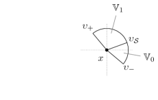
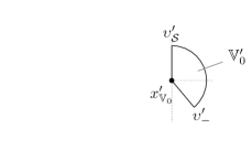
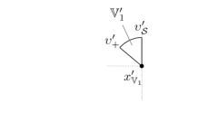
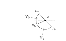
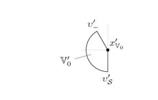
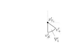
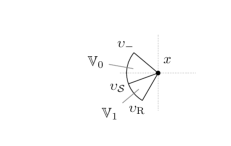
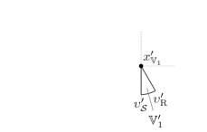
Figure 6. The three possible cutting cases for $\mathbb{V}$ by $\hat{\mathcal{S}}^{1}$ in regular sectors (on the left), and their images (on the right) by the two differentials $\mathcal{F}_{*,\mathbb{V}_{0}}$ and $\mathcal{F}_{*,\mathbb{V}_{1}}$ respectively.

In case (b), we necessarily have that $x\in\mathcal{S}^{+}_{\nu}$. We subdivide the argument into two further subcases: (i) $x\not\in\mathcal{S}_{\textup{R}}^{+}$; (ii) $x\in\mathcal{S}_{\textup{R}}^{+}.$

In case (i), $\mathcal{S}^{+}_{\nu}$ cuts $\mathbb{V}$ in exactly two sectors, induced by $\mathcal{D}^{+}_{\nu}$ and $\mathcal{D}^{+}_{\nu+1}$. Notice that these two sectors have a common boundary vector, which is induced by $\mathcal{S}^{+}_{\nu}$: we can then write the two sectors as (see Figure 6, first and second row) $\mathbb{V}_{0}=\mathbb{V}(\upsilon_{-},\upsilon_{\mathcal{S}})$ and $\mathbb{V}_{1}=\mathbb{V}(\upsilon_{\mathcal{S}},\upsilon_{+})$. We say we are in case $i^{\prime}$ if $\mathbb{V}$ contains the first quadrant (see first row of Figure 6) and in case $i^{\prime\prime}$ if $\mathbb{V}$ contains the third quadrant (see second row of Figure 6).

Consider first case $i^{\prime}$. By inspection we gather that $\mathbb{V}_{0}$ is induced by $\mathcal{D}^{+}_{\nu+1}$ and $\mathbb{V}_{1}$ is induced by $\mathcal{D}^{+}_{\nu}.$ Since we assume both sectors to be regular, Lemma 3.12(c) implies that

$$\lim_{y\to x}\mathcal{F}_{\mathbb{V}_{0}}x \in\{0\}\times\mathbb{R}^{+}, \lim_{y\to x}\mathcal{F}_{\mathbb{V}_{1}}x \in\{1\}\times\mathbb{R}^{+}.$$

Thus the image $\mathcal{F}_{*,\mathbb{V}_{0}}\upsilon_{\mathcal{S}}$ (resp. $\mathcal{F}_{*,\mathbb{V}_{1}}\upsilon_{\mathcal{S}}$) is a vertical vector. Moreover, since $\upsilon_{\mathcal{S}}$ lies in the first quadrant), then both its images are vertical vectors pointing upwards. The other boundary vector of each $\mathbb{V}_{i}$ is one of the original vectors $\upsilon_{\pm}$, and thus its image is unstable. Since $\mathcal{F}_{*,\mathbb{V}_{i}}$ is orientation preserving, we conclude that only one of the images of $\mathbb{V}_{i}$’s can be an active sector (see again Figure 6, row 1).

Case $i^{\prime\prime}$ is completely analogous. In this case $\mathbb{V}_{0}$ is induced by $\mathcal{D}^{+}_{\nu}$ and $\mathbb{V}_{1}$ is induced by $\mathcal{D}^{+}_{\nu+1}$. Once again, since both sectors are regular, we gather by Lemma 3.12(c) that

$$\lim_{y\to x}\mathcal{F}_{\mathbb{V}_{0}}x \in\{1\}\times\mathbb{R}^{+} \lim_{y\to x}\mathcal{F}_{\mathbb{V}_{1}}x \in\{0\}\times\mathbb{R}^{+}.$$

Hence the image $\mathcal{F}_{*,\mathbb{V}_{0}}\upsilon_{\mathcal{S}}$ (resp. $\mathcal{F}_{*,\mathbb{V}_{1}}\upsilon_{\mathcal{S}}$) is a vertical vector. Moreover, since $\upsilon_{\mathcal{S}}$ lies in the third quadrant, then both its images are vertical vectors pointing downwards. The other boundary vector of each $\mathbb{V}_{i}$ is one of the original vectors $\upsilon_{\pm}$, and thus its image is unstable . Since $\mathcal{F}_{*,\mathbb{V}_{i}}$ is orientation preserving, we conclude that only one of the images of $\mathbb{V}_{i}$’s can be an active sector (see Figure 6, second row). This completes the proof in case (i).

In case (ii), combining Lemma 3.10 (we need the part concerning $\mathcal{S}^{+}$!) with Lemma 3.6 we gather that $x$ is the right endpoint of $\mathcal{S}^{+}_{\nu}$. Therefore $\mathcal{S}^{+}_{\nu}$ will cut $\mathbb{V}$ only if $\mathbb{V}$ contains the third quadrant. Thus, if $\mathbb{V}$ contains the first quadrant, then $\mathcal{S}^{+}_{\nu}$ does not cut $\mathbb{V}$. Thus $\mathbb{V}$ could only be cut by $\mathcal{S}_{\textup{R}}^{+}$ and by an earlier discussion $\mathbb{V}$ contains at most one regular sector, so we are done.

It remains to consider the more difficult case in which $\mathbb{V}$ contains the third quadrant (Figure 6, bottom row). Since $x$ is the right endpoint of $\mathcal{S}^{+}_{\nu}$, we conclude that the vector induced by $\mathcal{S}^{+}_{\nu}$ must meet with $\mathcal{S}_{\textup{R}}^{+}$ on the left. Therefore the two regular sectors are $\mathbb{V}_{0}=\mathbb{V}(\upsilon_{-},\upsilon_{\mathcal{S}})$ and $\mathbb{V}_{1}=\mathbb{V}(\upsilon_{\mathcal{S}},\upsilon_{\textup{R}})$. As in case $i^{\prime\prime},$ we have that $\mathbb{V}_{0}$ is induced by $\mathcal{D}^{+}_{\nu}$ and $\mathbb{V}_{1}$ is induced by $\mathcal{D}^{+}_{\nu+1}$; the vector $\upsilon_{\textup{R}}$ is induced by $\mathcal{S}_{\textup{R}}^{+}$. Following the same reasoning as in case $i^{\prime\prime}$ above, we conclude that the image $\mathcal{F}_{*,\mathbb{V}_{0}}\upsilon_{\mathcal{S}}$ (resp. $\mathcal{F}_{*,\mathbb{V}_{1}}\upsilon_{\mathcal{S}}$) is a vertical vector pointing downwards. The image $\mathcal{F}_{*,\mathbb{V}_{0}}\upsilon_{-}$ is of course unstable and belongs to the second quadrant. The image of $\upsilon_{\textup{R}}$ is also in ${\mathfrak{N}}$ (as it will be induced by some curve in $\mathcal{S}^{-1}$) and points downwards. Hence, only $\mathbb{V}_{0}^{\prime}$ is active.

This concludes the argument in case (ii) and finishes the proof. ∎

7. Invariant manifolds.

The expansion estimate proved in the previous section is the main ingredient for the so-called Growth Lemma (Lemma 7.2). In turn the Growth Lemma constitutes the backbone for proving ergodicity using the Hopf argument, as will be done in the next section. The Hopf argument relies on existence of a large set of points which have sufficiently long stable and unstable manifolds. The present section contains necessary results about the existence of stable and unstable manifolds as well as regularity of partition of the phase space into stable and unstable manifolds. In this section we always assume that the Fermi–Ulam model is regular at infinity. As a notational convention, in an attempt to simplify our notation, in this section we drop the superscripts from $d_{\alpha}^{W}(\cdot,\cdot)$, as they can be unambiguously recovered from the context.

7.1. The Growth Lemma

In this section we state and prove a version of the Growth Lemma for our system. This lemma will allow to obtain, in the next subsection, a good lower bound on the length of stable and unstable manifolds passing through most of the points.

Let $W$ be an unstable curve and $x\in W$. $x$ subdivides $W$ into two subcurves. We define $r_{W}(x)$ as the $\alpha$-length of the shortest of the two subcurves. The function $r_{W}(x)$ measures, in an appropriate way, the distance of $x$ to the boundary of $W$. Observe that if $W$ is weakly homogeneous, we have, by (4.38),  $r_{W}(x)<C_{\#}d_{\alpha}(x,\mathbb{S})$.

Observe moreover that

(7.1) $$\textup{Leb}_{W}(r_{W}(x)<\varepsilon)=\min\{2\varepsilon,\textup{Leb}_{W}(W)\}$$

(recall that $\textup{Leb}_{W}$ denotes Lebesgue measure on the curve $W$ with respect to the $\alpha$-metric).

Given an unstable curve $W,$ a point $x\in W$ and $n\geq 0$, we define $W_{n}(x)$ as follows. If $x\in{\mathcal{S}}_{\mathbb{H}}^{n}$ we let $W_{n}(x)=\emptyset$; otherwise we let $W_{n}(x)$ to be the H-component of $\mathcal{F}^{n}W$ that contains $\mathcal{F}^{n}x$ (recall the discussion before Proposition 6.5). Then we define $r_{W,n}(x)=r_{W_{n}(x)}(\mathcal{F}^{n}x)$ (or $0$ if $W_{n}(x)=\emptyset$).

Likewise, given an unstable curve $W$, $x\in W$ and $n\geq 0$, we define $\widehat{W}_{n}(x)$ and $\hat{r}_{W,n}$ as follows. Recall the definition of $\hat{N}_{n}$ given before Remark 4.3; if $\hat{N}_{n}(x)$ is not defined, we let $\widehat{W}_{n}(x)=\emptyset$ and $\hat{r}_{W,n}(x)=0$. Otherwise we let $\widehat{W}_{n}(x)=W_{\hat{N}_{n}(x)}(x)$ and $\hat{r}_{W,n}(x)=r_{W,\hat{N}_{n}(x)}(x)$.

Lemma 7.1.

We have $r_{W,0}=\hat{r}_{W,0}=r_{W}$ and

(7.2) $$r_{W,n}(x)<C_{\#}d_{\alpha}(\mathcal{F}^{n}x,\mathbb{S}).$$

Moreover, there exists $C>1$, so that if $\mathcal{F}^{n}W$ is a single H-component, then for any $x\in W$:

(7.3) $$r_{W,n}(x)>C^{-1}\Lambda^{\hat{n}(\mathcal{F}^{n}W)}r_{W}(x),$$

where $\Lambda$ is the constant appearing in (4.27) and $\hat{n}$ was defined in (4.6).

Proof.

The first two items follow immediately from the definition and from our previous observation. We thus need to prove (7.3). By definition $r_{W,n}(x)=|W^{\prime}_{n}(x)|_{\alpha}$, where $W^{\prime}_{n}(x)$ is shortest subcurve of $W_{n}(x)$ joining $x_{n}$ with $\partial W_{n}(x)$. Since $\mathcal{F}^{n}W$ is a single H-component, we conclude that $W_{n}(x)=\mathcal{F}^{n}W$. Thus $W^{\prime}_{n}(x)$ connects $x_{n}$ with $\partial\mathcal{F}^{n}W$, and $\mathcal{F}^{-n}W^{\prime}_{n}(x)$ connects $x$ with $\partial W$. In particular $|\mathcal{F}^{-n}W^{\prime}_{n}(x)|_{\alpha}\geq r_{W}(x)$. Then the proof follows from (4.39a), (4.27) and the definition of $\hat{n}$. ∎

The following is the classical Growth Lemma.

Lemma 7.2 (Growth Lemma for $\hat{r}$).

Suppose that the Fermi–Ulam model is regular at infinity. Then there exists $0<\theta<1$ and $C>0$ so that for any sufficiently short mature admissible unstable curve $W\subset\mathcal{M}$, any $\varepsilon>0$ and any $n>0$

(7.4) $$\textup{Leb}_{W}(\hat{r}_{W,n}(x)<\varepsilon)\leq C\varepsilon\,\textup{Leb}_{W}(W)+C\textup{Leb}_{W}\left(r_{W}(x)\leq\theta^{n}\varepsilon\right).$$

Proof.

The proof of the Growth Lemma follows via relatively standard arguments (see [9, Sections 5.9 and 5.10]) from the expansion estimate (Proposition 6.5) and the distortion bounds proved in Corollary 5.11.

Recall the definition of $\hat{\mathcal{L}}_{n}$ given right before Proposition 6.5, and let $\bar{n}$ be the number appearing in Proposition 6.5. We fix $\delta>0$ to be sufficiently small so that $\bar{\theta}=e^{2C_{\textup{D}}\delta^{1/12}}\hat{\mathcal{L}}_{\bar{n}}<1$ (where $C_{\textup{D}}$ is the constant appearing in Corollary 5.11) and that Lemma 4.20(b) holds with $k=\bar{n}$ and $\delta_{*}=1$.

Let us first assume that $W\subset\widehat{\mathcal{M}}$ and that $|W|_{\alpha}<\delta$. Then we claim that there exists $\bar{C}>0$ so that for any $\varepsilon>0$:

(7.5) $$\textup{Leb}_{W}(\hat{r}_{W,\bar{n}}(x)<\varepsilon)<\bar{C}\varepsilon\textup{Leb}W+\textup{Leb}_{W}(r_{W}(x)<e^{-C_{\textup{D}}\delta^{1/12}}\bar{\theta}\varepsilon).$$

As we observed in Corollary 5.11, our distortion bounds on unstable curves depend on their length. In this proof we will need very fine distortion bounds, and it will then be necessary to work only with sufficiently short unstable curves. This entails a partitioning scheme for H-components that we now proceed to describe. Let $\{W_{i}\}$ denote the set of H-components of $\hat{\mathcal{F}}^{\bar{n}}W$. We partition each $W_{i}$ into a number

$$k_{i}=\left\lfloor\frac{|W_{i}|_{\alpha}}{\delta}\right\rfloor+1$$

of subcurves of equal $\alpha$-length (smaller than $\delta$) that we denote with $W_{ij}$. Observe that if $|W_{i}|_{\alpha}<\delta$, $k_{i}=1$, and no shortening takes place. We call such subcurves shortened H-components of $\hat{\mathcal{F}}^{\bar{n}}W$. We will shorten the H-components inductively every $\bar{n}$ steps of the induced map $\hat{\mathcal{F}}$. By our choice of $\delta$, this guarantees that at each intermediate step, no H-component will have $\alpha$-length exceeding $1$. Given $x\in W$, we will then denote with $\hat{W}^{\prime}_{n}(x)$ the shortened H-component of $\hat{\mathcal{F}}^{n}W$ whose interior contains $\hat{\mathcal{F}}^{n}x$ (or $\emptyset$ if some image of $x$ lies on an endpoint of a shortened subcurve). We then define $\hat{r}^{\prime}_{W,n}(x)=r_{\hat{W}^{\prime}_{n}(x)}(\hat{\mathcal{F}}^{n}x)$. Observe that $\hat{r}^{\prime}_{W,\bar{n}}<\hat{r}_{W,\bar{n}}$, so that proving (7.5) for $\hat{r}^{\prime}_{W,n}$ will imply (7.5) for $\hat{r}_{W,n}$. Let $B_{ij}\subset W_{ij}$ be the $\varepsilon$-neighborhood (in the $\alpha$-metric) of the boundary of each $W_{ij}$; in particular $\textup{Leb}_{W_{ij}}(B_{ij})=2\varepsilon$. Then

$$\textup{Leb}_{W}(\hat{r}^{\prime}_{W,\bar{n}}(x)<\varepsilon)=\sum_{ij}\textup{Leb}_{W}(\hat{\mathcal{F}}^{-\bar{n}}B_{ij}).$$

By the distortion estimates of Corollary 5.11

$$\sum_{ij}\textup{Leb}_{W}(\hat{\mathcal{F}}^{-\bar{n}}B_{ij}) \leq e^{C_{\textup{D}}\delta^{1/12}}\sum_{ij}\textup{Leb}_{W}(\hat{\mathcal{F}}^{-\bar{n}}W_{ij})\frac{\textup{Leb}_{W_{ij}}(B_{ij})}{\textup{Leb}_{W_{ij}}(W_{ij})}.$$

$$\leq 2e^{C_{\textup{D}}\delta^{1/12}}\varepsilon\sum_{ij}k_{i}\frac{\textup{Leb}_{W}(\hat{\mathcal{F}}^{-\bar{n}}W_{ij})}{\textup{Leb}_{W_{i}}(W_{i})}$$

$$\leq 2\delta^{-1}e^{C_{\textup{D}}\delta^{1/12}}\varepsilon\sum_{ij}\textup{Leb}_{W}(\hat{\mathcal{F}}^{-\bar{n}}W_{ij})+$$

$$\phantom{\leq}+2e^{C_{\textup{D}}\delta^{1/12}}\varepsilon\sum_{ij}\frac{\textup{Leb}_{W}(\hat{\mathcal{F}}^{-\bar{n}}W_{ij})}{\textup{Leb}_{W_{i}}(W_{i})}$$

$$\leq\bar{C}\varepsilon\textup{Leb}_{W}(W)+2e^{C_{\textup{D}}\delta^{1/12}}\varepsilon\sum_{i}\frac{\textup{Leb}_{W}(\hat{\mathcal{F}}^{-\bar{n}}W_{i})}{\textup{Leb}_{W_{i}}(W_{i})}$$

$$\leq\bar{C}\varepsilon\textup{Leb}_{W}(W)+2e^{C_{\textup{D}}\delta^{1/12}}\varepsilon\hat{\mathcal{L}}_{\bar{n}},$$

where we defined $\bar{C}=2\delta^{-1}e^{C_{\textup{D}}\delta^{1/12}}$. Using (7.1), the fact that the left hand side is always bounded above by $\textup{Leb}_{W}$, and our definition of $\bar{\theta}$, we conclude that

(7.6) $$\textup{Leb}_{W}(\hat{r}^{\prime}_{W,\bar{n}}(x)<\varepsilon)<\bar{C}\varepsilon\textup{Leb}W+\textup{Leb}_{W}(r_{W}(x)<e^{-C_{\textup{D}}\delta^{1/12}}\bar{\theta}\varepsilon).$$

which, as noted earlier, implies (7.5).

We now proceed to show that for any $k>0$:

(7.7) $$\textup{Leb}_{W}(\hat{r}^{\prime}_{W,k\bar{n}}(x)<\varepsilon) \leq e^{C_{\textup{D}}\delta^{1/12}}\frac{1-\bar{\theta}^{k}}{1-\bar{\theta}}\cdot\bar{C}\varepsilon\textup{Leb}_{W}(W)+$$

$$\phantom{=}+\textup{Leb}_{W}(r_{W}(x)\leq\bar{\theta}^{k}\varepsilon).$$

For $k=1$ (7.7) follows from (7.6). Let us assume by induction that (7.7) holds for $k$ and prove it for $k+1$. Let $W^{\prime}$ be a shortened H-component of $\hat{\mathcal{F}}^{k\bar{n}}$. Notice that by construction $W^{\prime}\subset\widehat{\mathcal{M}}$ and $|W^{\prime}|_{\alpha}<\delta$. Then, applying (7.5) to $W^{\prime}$ we gather:

$$\textup{Leb}_{W^{\prime}}(\hat{r}^{\prime}_{W^{\prime},\bar{n}}(y)<\varepsilon) \leq\bar{C}\varepsilon\textup{Leb}_{W^{\prime}}(W^{\prime})+\textup{Leb}_{W^{\prime}}(\hat{r}_{W^{\prime}}(y)\leq e^{-C_{\textup{D}}\delta^{1/12}}\bar{\theta}\varepsilon).$$

Let $W^{\prime\prime}=\hat{\mathcal{F}}^{-k\bar{n}}$, then by Corollary 5.11, we conclude that:

$$\textup{Leb}_{W^{\prime\prime}}(\hat{r}^{\prime}_{W^{\prime\prime},(k+1)\bar{n}}(x)<\varepsilon) \leq e^{C_{\textup{D}}\delta^{1/12}}\bar{C}\varepsilon\textup{Leb}_{W^{\prime\prime}}(W^{\prime\prime})$$

$$\phantom{=}+e^{C_{\textup{D}}\delta^{1/12}}\textup{Leb}_{W^{\prime\prime}}(\hat{r}^{\prime}_{W^{\prime\prime},k\bar{n}}(x)<e^{-C_{\textup{D}}\delta^{1/12}}\bar{\theta}\varepsilon).$$

Summing over all $W^{\prime\prime}$’s and applying the inductive hypothesis yields:

$$\textup{Leb}_{W}(\hat{r}^{\prime}_{W,(k+1)\bar{n}}(x)<\varepsilon)\leq$$

$$e^{C_{\textup{D}}\delta^{1/12}}\bar{C}\varepsilon\textup{Leb}_{W}(W)+e^{C_{\textup{D}}\delta^{1/12}}\textup{Leb}_{W}(\hat{r}^{\prime}_{W,k\bar{n}}(x)<e^{-C_{\textup{D}}\delta^{1/12}}\bar{\theta}\varepsilon)\leq$$

$$e^{C_{\textup{D}}\delta^{1/12}}\bar{C}\frac{1-\bar{\theta}^{k+1}}{1-\bar{\theta}}\varepsilon\textup{Leb}_{W}(W)+e^{C_{\textup{D}}\delta^{1/12}}\textup{Leb}_{W}(r_{W}(x)<e^{-C_{\textup{D}}\delta^{1/12}}\bar{\theta}^{k+1}\varepsilon),$$

which yields (7.7) for $k+1$. Hence we can write:

(7.8) $$\textup{Leb}_{W}(\hat{r}^{\prime}_{W,k\bar{n}}(x)<\varepsilon)\leq C\varepsilon\textup{Leb}_{W}(W)+\textup{Leb}_{W}(r_{W}(x)\leq\bar{\theta}^{k}\varepsilon).$$

where $C=\ifrac{\bar{C}e^{C_{\textup{D}}\delta^{1/12}}}{(1-\theta)}$.

We now extend this estimate to iterates that are not multiples of $\bar{n}$. We begin by obtaining a bound on $\textup{Leb}_{W}(\hat{r}^{\prime}_{W,s}(x)<\varepsilon)$ for $s<\bar{n}$. Notice that no partitioning into short curves occurs before step $\bar{n}$, therefore if $\{W_{i}\}$ denotes the set of $H$-component of $\hat{\mathcal{F}}^{s}W$, we have

$$\textup{Leb}_{W}(\hat{r}^{\prime}_{W,s}(x)<\varepsilon)=\textup{Leb}_{W}(\hat{r}_{W,s}(x)<\varepsilon)=\sum_{i}\textup{Leb}_{W}(\hat{\mathcal{F}}^{-s}B_{i}),$$

where $B_{i}$ is a $\varepsilon$-neighborhood of the boundary of $W_{i}$. Then we proceed as before. Since $|W|_{\alpha}<\delta$, we are guaranteed that $|W^{\prime}|_{\alpha}<1$. Thus, applying the distortion bounds in Corollary 5.11, we gather:

$$\sum_{i}\textup{Leb}_{W}(\hat{\mathcal{F}}^{-s}B_{i}) \leq 2e^{C_{\textup{D}}}\varepsilon\sum_{i}\frac{\textup{Leb}_{W}(\hat{\mathcal{F}}^{-s}W_{i})}{\textup{Leb}_{W_{i}}(W_{i})}\leq 2e^{C_{\textup{D}}}\varepsilon\hat{\mathcal{L}}_{s}.$$

Applying once again (7.1), and observing that by Proposition 6.5 we have that $\hat{\mathcal{L}}_{s}$ is bounded uniformly in $s$, yields:

(7.9) $$\textup{Leb}_{W}(\hat{r}_{W,s}(x)<\varepsilon)\leq\textup{Leb}_{W}(r_{W}(x)<C_{\#}\varepsilon).$$

Now, for any $m>0$, we write $m=k\bar{n}+s$, with $0\leq s<\bar{n}$. Applying (7.9) to each shortened component $W^{\prime}$ of $\hat{\mathcal{F}}^{k\bar{n}}W$ yields:

$$\textup{Leb}_{W^{\prime}}(\hat{r}_{W^{\prime},s}(y)<\varepsilon)\leq\textup{Leb}_{W^{\prime}}(r_{W^{\prime}}(x)<C_{\#}\varepsilon).$$

Taking $W^{\prime\prime}=\hat{\mathcal{F}}^{-k\bar{n}}W^{\prime}\subset W$, and applying the distortion bounds:

$$\textup{Leb}_{W^{\prime\prime}}(\hat{r}_{W^{\prime\prime},k\bar{n}+s}(x)<\varepsilon) \leq e^{C_{\textup{D}}\delta^{1/12}}\textup{Leb}_{W^{\prime\prime}}(r^{\prime}_{W^{\prime\prime},k\bar{n}}(x)<C_{\#}\varepsilon).$$

Now summing over all $W^{\prime\prime}$ and applying (7.8), we finally conclude that

$$\textup{Leb}_{W}(\hat{r}_{W,k\bar{n}+s}(x)<\varepsilon) \leq e^{C_{\textup{D}}\delta^{1/12}}C\varepsilon\textup{Leb}_{W}(W)+\textup{Leb}_{W}(r_{W}(x)\leq C_{\#}\bar{\theta}^{k}\varepsilon).$$

Choosing $\theta=\bar{\theta}^{1/\bar{n}}$ and $C=C_{\#}\theta^{-1}$ yields (7.4) under the assumption $W\subset\widehat{\mathcal{M}}$ and $|W|_{\alpha}<\delta$.

Now, observe that, given an unstable curve $W$, for any $x\in W$, $\hat{W}_{1}(x)$ is either $\emptyset$ or it is a curve $W^{\prime}\subset\widehat{\mathcal{M}}$. By Lemma 4.20, it is possible to assume $W$ so short that each $W^{\prime}$ is such that $|W^{\prime}|_{\alpha}<\delta$. By applying once again the distortion argument, we deduce that (7.4) holds in the general case, by suitably increasing the constants. ∎

We are now going to complement the Growth Lemma above (which involves iterates of $W$ by $\hat{\mathcal{F}}$) with some estimates on the length of the iterates of unstable curves by $\mathcal{F}$. More precisely, let $W$ be an unstable curve and $x\in W$: we define:

$$\bar{r}_{W}(x)=\min_{0\leq n<\hat{N}(x)}r_{W,n}(x),$$

with the convention that if $\hat{N}(x)$ is undefined, then $\bar{r}_{W}(x)=0$.

Lemma 7.3 (Transient growth control).

There exists $C>0$ so that for any sufficiently short mature admissible unstable curve $W$:

$$\textup{Leb}_{W}(\bar{r}_{W}(x)<\varepsilon)<\textup{Leb}_{W}(r_{W}(x)<C\varepsilon).$$

Proof.

The proof follows from distortion arguments similar to the ones given in the proof of the Growth Lemma. Assume that $|W|_{\alpha}<\delta$. Fix $w_{*}>0$ sufficiently large. Assume first that $W\subset\{w\leq w_{*}\}$. Then there exists $N_{*}=C_{\#}w_{*}$ so that $\hat{N}(x)<N_{*}$ for any $x\in W$. Thus:

$$\textup{Leb}_{W}(\bar{r}_{W}(x)<\varepsilon) \leq\sum_{n=0}^{N_{*}-1}\textup{Leb}_{W}(r_{W,n}(x)<\varepsilon).$$

We proceed to obtain a bound on $\textup{Leb}_{W}(r_{W,n}(x)<\varepsilon)$. Let us fix $n>0$ and let $\{W_{i}\}$ denote the set of H-components of $\mathcal{F}^{n}W$; let $B_{i}$ be an $\varepsilon$-neighborhood of the boundary of $W_{i}$. Then

$$\textup{Leb}_{W}(r_{W,n}(x)<\varepsilon)=\sum_{i}\textup{Leb}_{W}(\mathcal{F}^{-n}B_{i}).$$

Assuming $|W|_{\alpha}<\delta$, we are guaranteed that each component $W_{i}$ satisfies $|W_{i}|_{\alpha}<1$. Hence by our distortion bounds (Corollary 5.11)

$$\sum_{i}\textup{Leb}_{W}(\mathcal{F}^{-n}B_{i}) \leq 2e^{C_{\textup{D}}}\varepsilon\sum_{i}\frac{\textup{Leb}_{W}(\mathcal{F}^{-n}W_{i})}{\textup{Leb}_{W}(W_{i})}$$

$$\leq 2e^{C_{\textup{D}}}\varepsilon\mathcal{L}_{n}(W)$$

$$\leq\textup{Leb}_{W}(r_{W}(x)<e^{C_{\textup{D}}}\mathcal{L}_{n}\varepsilon).$$

By (6.3), $\mathcal{L}_{n}\leq\mathcal{L}_{1}^{n}.$ Thus $\mathcal{L}_{n}\leq\max\{1,\mathcal{L}_{1}^{N_{*}}\}$, which is bounded by (6.8). This concludes the proof of the lemma in the case of low energies.

Let us assume, on the other hand, that $W\cap\{w>w_{*}\}\neq\emptyset$. Then if $w_{*}$ is sufficiently large and $\delta$ sufficiently small, by Lemma 4.22(b), $W$ intersects at most two cells $\mathcal{E}^{*}_{n}$. Such cells partition $W$ in (at most) two subcurves $W_{1}$ and $W_{2}$ so that $\hat{N}(x)=N_{*}$ for all $x\in W_{1}$ and $\hat{N}(x)=N_{*}+1$ for all $x\in W_{2}$, for some $N_{*}>0$. Note that

$$\textup{Leb}_{W}(\bar{r}_{W}(x)<\varepsilon)\leq\textup{Leb}_{W}(\bar{r}_{W_{1}}(x)<\varepsilon)+\textup{Leb}_{W}(\bar{r}_{W_{2}}(x)<\varepsilon).$$

Let us consider $\bar{r}_{W_{1}}(x)$; by construction $W_{1}\subset\mathcal{E}^{*}_{N_{*}}$. Since $\mathcal{E}^{*}_{N_{*}}\cap\mathcal{S}^{N_{*}-1}=\emptyset$, we gather that $\mathcal{F}^{n}W_{1}$ is connected for any $0\leq n<N_{*}$. Thus, (7.3) ensures that $r_{W_{1},n}(x)\leq C^{-1}r_{W_{1}}(x)$ for any $n<N_{*}$, and therefore $\bar{r}_{W_{1}}(x)<C^{-1}r_{W_{1}}(x)$. By the same token we conclude $\bar{r}_{W_{2}}(x)<C^{-1}r_{W_{2}}(x)$. Hence

$$\textup{Leb}_{W}(\bar{r}_{W}(x)<\varepsilon)\leq\textup{Leb}_{W}(r_{W}<2C\varepsilon)$$

which concludes the proof of the lemma. ∎

In order to obtain bounds on the length of stable and unstable manifolds, we will need some results similar to the ones presented above, but for slightly different functions $r$. We now proceed to define them and link their properties to the ones of the functions $r$ that have been investigated above.

Recall the properties of the singularity sets $\mathcal{S}^{\pm}$ outlined in Lemma 3.10 and define, for $N\geq 0$:

$$\mathcal{S}^{+}_{(N)} =\mathcal{S}^{0}\cup\mathcal{S}^{+}_{\textup{R}}\cup\bigcup_{\nu=0}^{N}\mathcal{S}^{+}_{\nu}.$$

For $x\in W$ let us define $r_{W}(x,\mathcal{S}^{+}_{(N)})$ as follows. If $x\in\mathcal{S}^{+}_{(N)}$ we set $r_{W}(x,\mathcal{S}^{+}_{(N)})=0$. Otherwise $\mathcal{S}^{+}_{(N)}$ cuts $W$ into finitely many subcurves. Let $W^{\prime}$ be the subcurve that contains $x$ and $r_{W}(x,\mathcal{S}^{+}_{(N)})=r_{W^{\prime}}(x)$. Observe that necessarily $r_{W}(x,\mathcal{S}^{+}_{(N)})\leq r_{W}(x)$. Finally define

$$r_{W}^{*}(x)=\inf_{N>0}\{N^{3/2}r_{W}(x,\mathcal{S}^{+}_{(N)})\}.$$

Notice that $r^{*}_{W}(x)\leq r_{W}(x)$, and it could, in principle, be much smaller than $r_{W}$. However, the measure of points where this possibility occurs is under control thanks to the following bound.

Lemma 7.4.

There exists $C>0$ so that for any unstable curve $W$

$$\textup{Leb}_{W}(r^{*}_{W}(x)<\varepsilon)\leq\textup{Leb}_{W}(r_{W}(x)<C\varepsilon).$$

Proof.

By Lemma 3.10, we conclude that the set $\{r_{W}^{*}(x)<\varepsilon\}$ is contained in the union of

• 2 intervals of $\alpha$-length $\varepsilon$ at the boundary of $W$

• an interval of $\alpha$-length $2\varepsilon$ centered at each point of $W\cap(\mathcal{S}^{+}_{\textup{R}}\cup\mathcal{S}^{+}_{0})$;

• an interval of $\alpha$-length $2\nu^{-3/2}\varepsilon$ centered at each point of $W\cap\mathcal{S}^{+}_{\nu}$ for $\nu>0$.

Hence

$$\textup{Leb}_{W}(r_{W}^{*}(x)<\varepsilon)<2\varepsilon(1+2+\sum_{\nu>0}\nu^{-3/2})<2C_{\#}\varepsilon.$$

Since by definition $\textup{Leb}_{W}(r_{W}^{*}(x)<\varepsilon)\leq\textup{Leb}_{W}(W)$, we conclude that

$$\textup{Leb}_{W}(r_{W}^{*}(x)<\varepsilon) \leq\textup{Leb}_{W}(r_{W}(x)<C\varepsilon).\qed$$

Using the above lemma, it is possible to obtain a Growth Lemma and transient growth control for $r^{*}$. Let $W$ be an unstable curve and $x\in W$. For $n\geq 0$ we define $r^{*}_{W,n}(x)$ as follows; if $x\in{\mathcal{S}}_{\mathbb{H}}^{n}$ we let $r^{*}_{W,n}(x)=0$; otherwise $W_{n}(x)\neq\emptyset$ and we set

$$r^{*}_{W,n}(x)=r^{*}_{W_{n}(x)}(\mathcal{F}^{n}x).$$

Likewise, given $n\geq 0$, if $\hat{N}_{n}(x)$ is not defined, we let $\hat{r}^{*}_{W,n}(x)=0$. Otherwise we define

(7.10) $$\hat{r}^{*}_{W,n}(x)=r^{*}_{W,\hat{N}_{n}(x)}(x).$$

Finally, let $x\in W$. If $\hat{N}(x)$ is undefined, we let $\bar{r}^{*}_{W}(x)=0$. Otherwise let

$$\bar{r}^{*}_{W}(x) =\min_{0\leq n<\hat{N}(x)}r^{*}_{W,n}(x).$$

We now prove for $\bar{r}^{*}$ the same bound that was proved in Lemma 7.3.

Lemma 7.5.

There exists $C>0$ so that for any sufficiently short mature admissible unstable curve $W\subset\mathcal{M}$

(7.11) $$\textup{Leb}_{W}(\bar{r}^{*}_{W}(x)<\varepsilon) <\textup{Leb}_{W}(r_{W}(x)<C\varepsilon).$$

Proof.

Assume $|W|_{\alpha}<\delta$ and fix $w_{*}>0$ sufficiently large. Assume first that $W\subset\{w\leq w_{*}\}$. Then there exists $N_{*}=C_{\#}w_{*}$ so that $\hat{N}(x)<N_{*}$ for any $x\in W$. Thus:

$$\textup{Leb}_{W}(\bar{r}^{*}_{W}(x)<\varepsilon)\leq\sum_{n=0}^{N_{*}-1}\textup{Leb}_{W}(r^{*}_{W,n}(x)<\varepsilon).$$

Lemma 7.4 then implies that

$$\textup{Leb}_{W}(\bar{r}_{W}^{*}(x)<\varepsilon)\leq\sum_{n=0}^{N_{*}-1}\textup{Leb}_{W}(r_{W,n}(x)<C\varepsilon).$$

Now arguing as in the proof of Lemma 7.3, we conclude that (7.11) holds in this first case.

Assume now that $W\cap\{w>w_{*}\}\neq\emptyset$, then if $\delta$ is sufficiently small and $w_{*}$ sufficiently large, we conclude by Lemma 4.4(a) that for any $x\in W$ and any $0\leq n<\hat{N}(x)$, $\mathcal{F}^{n}x\in\{w\geq w_{*}/2\}$. First of all notice that Lemma 3.10 and the construction of $\mathcal{E}^{*}_{n}$ guarantees that $\mathcal{E}^{*}_{n}\cap\mathcal{S}^{+}=\emptyset$ unless $n=1$. By Lemma 3.10(d) $\mathcal{S}^{+}_{\nu}$ is compact for $\nu>0$. Therefore for large enough $w_{*}$, the only possible curve of $\mathcal{S}^{+}$ that intersects with $\mathcal{E}^{*}_{0}\cap\{w\geq w_{*}/2\}$ is $\mathcal{S}^{+}_{0}$, but $\mathcal{S}^{+}_{0}\subset\partial\mathcal{E}^{*}_{0}$; we conclude that $\mathcal{E}^{*}_{0}\cap\{w\geq w_{*}/2\}\cap\mathcal{S}^{+}=\emptyset$. We thus proceed as in the proof of Lemma 7.3: If $w_{*}$ is sufficiently large and $\delta$ sufficiently small, by Lemma 4.22(b), $W$ intersects at most two cells $\mathcal{E}^{*}_{n}$; such cells partition $W$ in (at most) two subcurves $W_{1}$ and $W_{2}$. Then

$$\textup{Leb}_{W}(\bar{r}^{*}_{W}(x)<\varepsilon) \leq\textup{Leb}_{W}(\bar{r}^{*}_{W_{1}}(x)<\varepsilon)+\textup{Leb}_{W}(\bar{r}^{*}_{W_{2}}(x)<\varepsilon).$$

Notice that $\mathcal{F}^{n}W_{i}$ will belong to only one cell $\mathcal{E}^{*}_{\nu}$ for any $n$ involved in the definition of $\bar{r}^{*}_{W_{i}}$. By the argument above, we gather that $\bar{r}^{*}_{W_{i}}=\bar{r}_{W_{i}}$. Now we conclude arguing as in the proof of Lemma 7.3. ∎

7.2. Size of invariant manifolds.

Recall that a stable curve $W$ is a homogeneous stable manifold if $|\mathcal{F}^{n}W|_{\alpha}\to 0$ as $n\to\infty$ and $\mathcal{F}^{n}W$ belongs to a single homogeneity strip for any $n\geq 0$. Recall also the corresponding definition for unstable manifolds. Given $x\in\mathcal{M}$, we denote with $W^{\text{s}}(x)$ (resp. $W^{\text{u}}(x)$) the maximal homogeneous stable (resp. unstable) manifold containing $x$ (or $\emptyset$ if such manifold does not exists). Conventionally we consider such curves without the endpoints. We now give a convenient characterization of $W^{\text{s}}(x)$ and $W^{\text{u}}(x)$. The construction closely follows [9, Section 4.11], and we refer the reader to that section for additional details. For $x\in\mathcal{M}\setminus{\mathcal{S}}_{\mathbb{H}}^{-\infty}$, we denote with $Q_{-n}(x)$ the connected component of the open set $\mathcal{M}\setminus{\mathcal{S}}_{\mathbb{H}}^{-n}$ that contains $x$. Naturally, $Q_{-n}(x)\supset Q_{-(n+1)}(x)$ for any $n$. Moreover $\overline{Q_{-n}}(x)$ is compact for any $n$ sufficiently large, possibly depending on $x$. Let $\widetilde{W}^{\text{u}}(x)=\bigcap_{n\geq 1}\overline{Q_{-n}(x)}$. Using compactness of $\overline{Q_{-n}(x)}$ and Lemma 4.23 one can show that $\widetilde{W}^{\text{u}}(x)$ is a compact unstable curve. It then follows that $W^{\text{u}}(x)$ is equal to $\widetilde{W}^{\text{u}}(x)$ minus the endpoints. A completely similar construction can be carried over for $W^{\text{s}}(x)$.

If $W^{\text{u}}(x)=\emptyset$ we define $r_{\text{u}}(x)=0$. Otherwise, $x$ subdivides $W^{\text{u}}(x)$ in two subcurves; we denote with $r_{\text{u}}(x)$ the $\alpha$-length of the shortest of such subcurves. Define $r_{\text{s}}(x)$ similarly.

We now obtain lower bounds for $r_{\text{s}}$ and $r_{\text{u}}$. In order to do so we introduce some notation. Given $x\in\mathcal{M}$, define the functions $E^{\pm}:\mathcal{M}\to\mathbb{R}$ so that if $x\in\mathbb{H}_{k}\cap\mathcal{D}^{\pm}_{\nu}$, then $E^{\pm}(x)=(\nu+1)(k^{2}+1)$. More precisely

$$E^{\pm}(x) =\sum_{k}(k^{2}+1)\chi_{\mathbb{H}_{k}\cap\mathcal{D}^{\pm}_{\textup{R}}}+\sum_{k,\nu}(k^{2}+1)(\nu+1)\chi_{\mathbb{H}_{k}\cap\mathcal{D}^{\pm}_{\nu}}(x),$$

where $\chi$ denotes the indicator function of the set written as its subscript.

Lemma 7.6.

$E^{\pm}$ controls the contraction and expansion of stable and unstable vectors by $d\mathcal{F}$ as follows:

(7.12a) $$C^{-1}E^{-}(\mathcal{F}x) <\frac{\|d\mathcal{F}v^{\text{u}}\|}{\|v^{\text{u}}\|}<CE^{-}(\mathcal{F}x) \forall\,x\in\mathcal{M}\setminus\mathcal{S}^{+},v^{\text{u}}\in\mathcal{C}^{\text{u}}_{x}$$

(7.12b) $$C^{-1}E^{+}(\mathcal{F}^{-1}x) <\frac{\|d\mathcal{F}^{-1}v^{\text{s}}\|}{\|v^{\text{s}}\|}<CE^{+}(\mathcal{F}^{-1}x) \forall\,x\in\mathcal{M}\setminus\mathcal{S}^{-},v^{\text{s}}\in\mathcal{C}^{\text{s}}_{x}.$$

Proof.

Of course it suffices to show(7.12a), then (7.12b) follows from the properties of the involution. If $\mathcal{F}x\in{\mathcal{D}^{-}_{\textup{R}}}$, then the lower bound follows from (4.25) and the upper bound follows from (4.29) and Corollary 4.11(a). On the other hand, suppose $\mathcal{F}x\not\in{\mathcal{D}^{-}_{\textup{R}}}$. If $w$ is large, then our estimates follow from Corollary 4.11 and (4.29). If $w$ is small, Lemma 4.8(b) and (4.29) yield the desired estimate. ∎

Given $x\in\mathcal{M}$ and $n\in\mathbb{Z}$, we denote with $d_{\alpha}^{\text{s}}(x,{\mathcal{S}}_{\mathbb{H}}^{n})$ (resp. $d_{\alpha}^{\text{u}}(x,{\mathcal{S}}_{\mathbb{H}}^{n})$) the length (in the $\alpha$-metric) of the shortest stable (resp. unstable) curve which connects $x$ with ${\mathcal{S}}_{\mathbb{H}}^{n}$.

For $x\in\mathcal{M}$, let $\Lambda^{\text{u}}_{n}(x)$ be the minimal expansion of unstable vectors by $d\mathcal{F}^{n}|_{x}$. Similarly, let $\Lambda^{\text{s}}_{n}(x)$ be the minimal expansion of stable vectors by $d\mathcal{F}^{-n}|_{x}$. Notice that there exists $\underline{\Lambda}>0$: so that for any $n>0$ and $x\in\mathcal{M}$

(7.13) $$\Lambda_{n}^{\text{s}}(x)>\underline{\Lambda},\quad\Lambda_{n}^{\text{u}}(x)>\underline{\Lambda}.$$

Moreover, by definition, for any $0<m<n$:

$$\Lambda^{\text{u}}_{n}(x) \geq\Lambda^{\text{u}}_{m}(x)\Lambda^{\text{u}}_{n-m}(\mathcal{F}^{m}x) \Lambda^{\text{s}}_{n}(x) \geq\Lambda^{\text{s}}_{m}(x)\Lambda^{\text{s}}_{n-m}(\mathcal{F}^{-m}x).$$

Hence by (7.12), there exists $c>0$ so that for any $n\geq 1$

(7.14a) $$\Lambda^{\text{u}}_{n}(x) \geq cE^{-}(\mathcal{F}x)\Lambda^{\text{u}}_{n-1}(\mathcal{F}x),$$

(7.14b) $$\Lambda^{\text{s}}_{n}(x) \geq cE^{+}(\mathcal{F}^{-1}x)\Lambda^{\text{s}}_{n-1}(\mathcal{F}^{-1}x).$$

Lemma 7.7.

For any $L>0$ there exists a constant $c>0$ such that

$$r_{\text{s}}(x) \geq\min\{L,c\inf_{n>0}\Lambda_{n}^{\text{s}}(\mathcal{F}^{n}x)d_{\alpha}^{\text{s}}(\mathcal{F}^{n}x,{\mathcal{S}}_{\mathbb{H}}^{-1})\},$$

$$r_{\text{u}}(x) \geq\min\{L,c\inf_{n>0}\Lambda_{n}^{\text{u}}(\mathcal{F}^{-n}x)d_{\alpha}^{\text{u}}(\mathcal{F}^{-n}x,{\mathcal{S}}_{\mathbb{H}}^{1})\}.$$

Proof.

The proof of the lemma is a combination of the arguments given in [9, Lemma 4.67, (4.61), Exercise 5.19 and (5.58)].

Let us prove the statement for $r_{\text{u}}$ (the statement for $r_{\text{s}}$ follows as usual by the properties of the involution). We may further assume that $x\in\mathcal{M}\setminus{\mathcal{S}}_{\mathbb{H}}^{-\infty}$ (otherwise the right hand side of the inequality is $0$ and the statement holds trivially). As before, for any $n$, we let $Q_{-n}(x)$ be the connected component of $\mathcal{M}\setminus{\mathcal{S}}_{\mathbb{H}}^{-n}$ containing the point $x$; clearly $Q_{n}(\mathcal{F}^{-n}x)=\mathcal{F}^{-n}(Q_{-n}(x))$ is the connected component of $\mathcal{M}\setminus{\mathcal{S}}_{\mathbb{H}}^{n}$ containing the point $\mathcal{F}^{-n}x$.

Let $n^{*}$ be so that $\overline{Q_{-n^{*}}(x)}$ is compact. Choose $w^{*}$ so that $\overline{Q_{-n^{*}}(x)}\subset\{w\leq w^{*}\}$. Let us now fix $\varepsilon>0$ and choose $n>n^{*}$ so that $\overline{Q_{-n}(x)}$ is contained in an Euclidean $\varepsilon/w^{*}$-neighborhood of $W^{\text{u}}(x)$.

By construction $\mathcal{F}^{-n}W^{\text{u}}(x)\subset Q_{n}(\mathcal{F}^{-n}x)$. Let $W^{\prime}_{-n}$ be an arbitrary continuation as a mature unstable curve of $\mathcal{F}^{-n}W^{\text{u}}(x)$ to $\partial Q_{n}(\mathcal{F}^{-n}x)$. We further assume that $W^{\prime}_{-n}$ is $\hat{K}$-admissible. Then $W^{\prime}=\mathcal{F}^{n}(W^{\prime}_{-n})$ is an unstable continuation of $W^{\text{u}}(x)$ that terminates on $\partial Q_{-n}(x)$. It is divided by the point $x$ into two subcurves; denote with $W$ the shortest one (in the $\alpha$-metric). By our construction and (4.16b) we gather that $r_{\text{u}}(x)\geq|W|_{\alpha}-C_{\#}\varepsilon$. Since $\varepsilon$ is arbitrary, it suffices to show that

$$|W|_{\alpha} \geq\min\{L,c\inf_{n>0}\Lambda_{n}^{\text{u}}(\mathcal{F}^{-n}x)d_{\alpha}^{\text{u}}(\mathcal{F}^{-n}x,{\mathcal{S}}_{\mathbb{H}}^{1})\}.$$

The above bound trivially holds if $|W|_{\alpha}\geq L$. Let us thus assume that $|W|_{\alpha}<L$ and for $0\leq m\leq n$ let $W_{-m}=\mathcal{F}^{-m}W$. Since $W_{-n}$ terminates on ${\mathcal{S}}_{\mathbb{H}}^{n}$, there exists $m\in[1,n]$ so that $W_{-m}$ joins $\mathcal{F}^{-m}x$ with ${\mathcal{S}}_{\mathbb{H}}^{1}$. We thus gather

$$|W|_{\alpha}=\frac{|W|_{\alpha}}{|W_{-m}|_{\alpha}}|W_{-m}|_{\alpha}\geq C_{\#}\Lambda_{m}^{\text{u}}(\mathcal{F}^{-m}x)|W_{-m}|_{\alpha}$$

$$\geq C_{\#}\Lambda_{m}^{\text{u}}(\mathcal{F}^{-m}x)d_{\alpha}^{\text{u}}(\mathcal{F}^{-m}x,{\mathcal{S}}_{\mathbb{H}}^{1})$$

where we used distortion estimates obtained in Corollary 5.11. ∎

The statement we are about to prove below (Lemma 7.8) is the analog of [9, Exercise 5.69], but there are some differences which are due to two separate issues. First of all the statement of that exercise is incorrect: the strategy presented in [9, Section 5.5] has a gap and needs to be corrected (see [3] for a proposed solution). Secondly, the argument would need a non-trivial adaptation to our specific case because of the nature of our singularities (presence of corner points, non-compactness). We thus proceed to give in detail the statement and the proof of what is needed for our analysis. In order to simplify our notation we denote, as usual, $x_{n}=\mathcal{F}^{n}x$.

Lemma 7.8.

There exists a constant $C>0$ so that

1. for any mature unstable curve $W\subset\mathcal{M}$, any $n\geq 2$ and any $x\in W\setminus\mathcal{S}^{n}$:

   (7.15a) $$\Lambda^{\text{s}}_{n}(x_{n})d_{\alpha}^{\text{s}}(x_{n},{\mathcal{S}}_{\mathbb{H}}^{-1})\geq C\min\{ \Lambda^{\text{s}}_{n}(x_{n})r_{W,n}(x),$$

   $$\Lambda^{\text{s}}_{n-1}(x_{n-1})r^{*}_{W,n-1}(x),$$

   $$\Lambda^{\text{s}}_{n-2}(x_{n-2})r_{W,n-2}(x)\}.$$

2. for any unstable curve $W\subset\mathcal{M}$ that is the image of a mature unstable curve and any $x\in W\setminus\mathcal{S}^{1}$:

   (7.15b) $$\Lambda^{\text{s}}_{1}(x_{1})d_{\alpha}^{\text{s}}(x_{1},{\mathcal{S}}_{\mathbb{H}}^{-1})\geq C\min\{ \Lambda^{\text{s}}_{1}(x_{1})r_{W,1}(x),r^{*}_{W}(x),r_{W}(x)^{4}\}.$$

Proof.

Recall that ${\mathcal{S}}_{\mathbb{H}}^{-1}$ is a closed set (see Remark 5.1). In particular $d_{\alpha}^{\text{s}}(x_{n},{\mathcal{S}}_{\mathbb{H}}^{-1})$ is attained as $|V|_{\alpha}$, where $V$ is a stable curve which joins $x_{n}$ to some point $z\in{\mathcal{S}}_{\mathbb{H}}^{-1}$. By definition (see (5.1)) we have:

$${\mathcal{S}}_{\mathbb{H}}^{-1}=\mathbb{S}\cup\mathcal{F}(\mathbb{S}\setminus\mathcal{S}^{+})\cup\mathcal{S}^{-}.$$

Hence there are three possibilities:

1. $z\in\mathbb{S}$;

2. $z\in\mathcal{F}(\mathbb{S}\setminus\mathcal{S}^{+})$;

3. $z\in\mathcal{S}^{-}$.

We begin with case (a). By definition it holds that $|V|_{\alpha}\geq d_{\alpha}(x_{n},\mathbb{S})$. Using (7.2) we thus conclude that $d_{\alpha}^{\text{s}}(x_{n},{\mathcal{S}}_{\mathbb{H}}^{-1})\geq cr_{W,n}(x)$.

In cases (b) and (c) we consider $V^{\prime}=\mathcal{F}^{-1}V$. Then $V^{\prime}$ is a weakly homogeneous stable curve and, by (7.12):

$$|V|_{\alpha}\geq\frac{c|V^{\prime}|_{\alpha}}{E^{+}(x_{n-1})}.$$

In case (b), $V^{\prime}$ links $x_{n-1}$ to some point $z^{\prime}\in\mathbb{S}$, therefore $|V^{\prime}|_{\alpha}\geq d_{\alpha}(x_{n-1},\mathbb{S})$ and using (7.14a) we gather that

$$\Lambda^{\text{s}}_{n}(x_{n})d_{\alpha}^{\text{s}}(x_{n},{\mathcal{S}}_{\mathbb{H}}^{-1}) \geq c\Lambda^{\text{s}}_{n-1}(x_{n-1})d_{\alpha}(x_{n-1},\mathbb{S}).$$

Using again (7.2) we thus conclude that

$$\Lambda^{\text{s}}_{n}(x_{n})d_{\alpha}^{\text{s}}(x_{n},{\mathcal{S}}_{\mathbb{H}}^{-1}) \geq c\Lambda^{\text{s}}_{n-1}(x_{n-1})r_{W,n-1}(x).$$

Finally, we consider case (c): then $V^{\prime}$ is a stable curve linking $x_{n-1}$ to some point $z^{\prime}\in\mathcal{S}^{+}$. We consider two possibilities:

1. $x_{n-1}\in{\mathcal{D}^{-}_{\textup{R}}}$ and $z^{\prime}\in\{0\}\times[0,\mathfrak{h}]$;

2. otherwise.

In case $(c^{\prime})$, observe that since $V^{\prime}$ is a stable curve, it is increasing, and the assumptions in $(c^{\prime})$ imply that $V^{\prime}\subset{\mathcal{D}^{-}_{\textup{R}}}$ (see Lemma 3.6). We have now to deal separately with the case $n=1$ and $n>1$. If $n>1$, consider $V^{\prime\prime}=\mathcal{F}^{-1}V^{\prime}$. Observe that $V^{\prime\prime}\subset{\mathcal{D}^{+}_{\textup{R}}}$ is a stable (once again, increasing) curve, which joins $x_{n-2}\in{\mathcal{D}^{+}_{\textup{R}}}$ to $z^{\prime\prime}\in\{r=1\}$. The expansion of $d\mathcal{F}^{-1}$ along $V^{\prime}$ is bounded above by $cE^{+}(x_{n-2})$ (since $x_{n-2}\in{\mathcal{D}^{+}_{\textup{R}}}$ and it is the lowest point on $V^{\prime\prime}$). We conclude that

$$|V^{\prime}|_{\alpha}\geq c\frac{|V^{\prime\prime}|_{\alpha}}{E^{+}(x_{n-2})}.$$

Hence, $|V^{\prime\prime}|_{\alpha}\geq d_{\alpha}(x_{n-2},\{r=1\})$. Now $x_{n-2}$ cuts $W_{n-2}(x)$ into two subcurves; let $W^{\prime}_{n-2}(x)$ denote the subcurve to the right of $x_{n-2}$; then by definition $|W^{\prime}_{n-2}(x)|\geq r_{W,n-2}(x)$. Notice that $W^{\prime}_{n-2}(x)\subset{\mathcal{D}^{+}_{\textup{R}}}$, thus $W^{\prime}_{n-2}(x)\cap{\mathcal{D}^{-}_{\textup{R}}}=\emptyset$; Corollary 4.11 then implies that we have uniform transversality of $W^{\prime}_{n-2}(x)$ with any vertical line, which allows to conclude that

$$d_{\alpha}{}(x_{n-2},\{r=1\}) \geq c|W^{\prime}_{n-2}(x)|_{\alpha}\geq cr_{W,n-2}(x).$$

Hence in case $(c^{\prime})$ and if $n>1$:

$$\Lambda^{\text{s}}_{n}(x_{n})d_{\alpha}^{\text{s}}(x_{n},{\mathcal{S}}_{\mathbb{H}}^{-1}) \geq C\Lambda^{\text{s}}_{n-2}(x_{n-2})r_{W,n-2}(x)\}.$$

Otherwise if $n=1$, we need to modify the above argument as follows. Applying Lemma 4.20 (and Remark 4.21) to the stable curve $V^{\prime}\subset{\mathcal{D}^{-}_{\textup{R}}}$ we conclude that

$$|V^{\prime}|_{\alpha}\geq c|V^{\prime\prime}|_{\alpha}^{2};$$

Then arguing as before (with $W_{n-2}$ replaced by $\mathcal{F}^{-1}W$, that is guaranteed to be a mature unstable curve by our assumption), we conclude that $|V^{\prime\prime}|_{\alpha}\geq cr_{\mathcal{F}^{-1}W}(x_{-1})$. Applying once again Lemma 4.20 (and Remark 4.21 to $\mathcal{F}^{-1}W$), we conclude that $r_{W}(x)\leq C_{\#}r_{\mathcal{F}^{-1}W}(x_{-1})^{1/2}$, from which we finally conclude that

$$r_{\text{s}}(x)=|V^{\prime}|_{\alpha}\geq Cr_{W}(x)^{4}.$$

We now estimate $|V^{\prime}|_{\alpha}$ in case $(c^{\prime\prime}).$ We claim that

(7.16) $$|V^{\prime}|_{\alpha}\geq C\inf_{N>0}N^{3/2}d(x_{n-1},\mathcal{S}^{+}_{(N)}).$$

The above holds trivially if $z^{\prime}\in\mathcal{S}^{+}_{(1)}$. Otherwise, there exists $\nu>1$ so that $z^{\prime}\in\mathcal{S}^{+}_{\nu}$. This implies that $V^{\prime}\subset\mathcal{D}^{+}_{\nu^{\prime}}$ where either $\nu^{\prime}=\nu$ or $\nu^{\prime}=\nu+1$. Since $\mathcal{D}^{+}_{\nu^{\prime}}$ is bounded if $\nu^{\prime}>1$ (see Lemma 3.12(e)), $V^{\prime}$ lies in a region where $w$ is bounded and so the $\alpha$-metric and the Euclidean metric are equivalent.

Moreover, the angle between $V^{\prime}$ and $\mathcal{S}^{+}_{\nu}$ is bounded above by $C\nu^{-3/2}$ (see the proof of Lemma 3.9). Thus $d_{\alpha}(x_{n-1},\mathcal{S}^{+}_{\nu})\leq C\nu^{-3/2}|V^{\prime}|_{\alpha}$. Since $d_{\alpha}(x_{n-1},\mathcal{S}^{+}_{(\nu)})\leq d_{\alpha}(x_{n-1},\mathcal{S}^{+}_{\nu})$, we obtain (7.16).

By Lemma 3.2 $\mathcal{S}^{+}_{(N)}$ is a union of curves compatible with the cone ${\mathfrak{P}}$. Moreover, since we are in case $(c^{\prime\prime})$, $x_{n-1}\not\in{\mathcal{D}^{-}_{\textup{R}}}$ (and thus $W_{n-1}(x)\cup{\mathcal{D}^{-}_{\textup{R}}}=\emptyset$). Hence by Corollary 4.11, $W_{n-1}$ is uniformly transversal to any curve in ${\mathfrak{P}}$ and we conclude that

$$d_{\alpha}(x_{n-1},\mathcal{S}^{+}_{(N)})\geq C_{\#}r_{W_{n-1}(x)}(x_{n-1},\mathcal{S}^{+}_{(N)}).$$

This yields

$$|V^{\prime}|_{\alpha}\geq C\inf_{N>0}N^{3/2}r_{W_{n-1}(x)}(x_{n-1},\mathcal{S}^{+}_{(N)})=Cr^{*}_{W,n-1}(x).$$

Therefore

$$\Lambda^{\text{s}}_{n}(x_{n})d_{\alpha}^{\text{s}}(x_{n},{\mathcal{S}}_{\mathbb{H}}^{-1}) \geq C\Lambda^{\text{s}}_{n-1}(x_{n-1})r^{*}_{W,n-1}(x)$$

concluding the proof. ∎

Using the two results bounds above it is possible to obtain lower bounds on the length of stable (resp. unstable) manifolds passing through most points on any given unstable (resp. stable) mature admissible curve. This is done in the following corollary, which is the analog to [9, Theorems 5.66–5.67, Section 5.12].

Corollary 7.9.

(a) There exists $C>0$ so that for any admissible mature unstable curve $W\subset\mathcal{M}$ and $\varepsilon>0$ with the property that for every $x\in W$ we have $d_{\alpha}(\mathcal{F}x,{\mathcal{S}}_{\mathbb{H}}^{-1})>C\varepsilon$, then

$$\textup{Leb}_{W}(r_{\text{s}}(x)\leq\varepsilon)<C_{\#}\varepsilon.$$

(a’) for any admissible mature unstable curve $W\subset\mathcal{M}$ that is the image of a mature unstable curve and any $\varepsilon>0$:

$$\textup{Leb}_{W}(r_{\text{s}}(x)\leq\varepsilon)<C_{\#}\varepsilon^{1/4}.$$

(b) for any $\eta>0$ there exists $k>0$ so that for any admissible mature unstable curve $W\subset\mathcal{M}$ and $\varepsilon>0$ with the property that for every $x\in W$ we have $d_{\alpha}(\mathcal{F}^{n}x,{\mathcal{S}}_{\mathbb{H}}^{-1})>\varepsilon$ for any $0\leq n\leq\hat{N}_{k}(x)$; then

(7.17) $$\textup{Leb}_{W}(r_{\text{s}}(x)\leq\varepsilon)\leq\eta\varepsilon.$$

(c) There exists $C>0$ so that for any admissible mature stable curve $W\subset\mathcal{M}$ and $\varepsilon>0$ with the property that for every $x\in W$ we have $d_{\alpha}(\mathcal{F}^{-1}x,{\mathcal{S}}_{\mathbb{H}}^{1})>C\varepsilon$, then

$$\textup{Leb}_{W}(r_{\text{u}}(x)\leq\varepsilon)<C_{\#}\varepsilon.$$

(c’) for any admissible mature stable curve $W\subset\mathcal{M}$ that is the pre-image of a mature stable curve and any $\varepsilon>0$:

$$\textup{Leb}_{W}(r_{\text{u}}(x)\leq\varepsilon)<C_{\#}\varepsilon^{1/4}.$$

(d) for any $\eta>0$ there exists $k>0$ so that for any admissible mature stable curve $W\subset\mathcal{M}$ and $\varepsilon>0$ with the property that for every $x\in W$ we have $d_{\alpha}(\mathcal{F}^{-n}x,{\mathcal{S}}_{\mathbb{H}}^{1})>\varepsilon$, for any $\hat{N}_{-k}(x)<n\leq 0$; then

$$\textup{Leb}_{W}(r_{\text{u}}(x)\leq\varepsilon) \leq\eta\varepsilon.$$

Proof.

We prove parts (a), (a’) and (b). Parts (c), (c’) and (d) follow by identical arguments by considering $\mathcal{F}^{-1}.$ Combining Lemmata  7.8 and  7.7 (with $L=1$) with the estimate $r_{W,n}(x)\geq r_{W,n}^{*}(x)$ we obtain

(7.18) $$r_{\text{s}}(x)\geq\min\{1,c\Lambda_{1}^{\text{s}}(\mathcal{F}x)d_{\alpha}^{\text{s}}(\mathcal{F}x,{\mathcal{S}}_{\mathbb{H}}^{-1}),C\inf_{n\geq 0}\Lambda_{n}^{\text{s}}(\mathcal{F}^{n}x)r_{W,n}^{*}(x)\}.$$

Define $C=c^{-1}\underline{\Lambda}^{-1}$ (recall (7.13)) to ensure that if $d_{\alpha}{}(\mathcal{F}x,{\mathcal{S}}_{\mathbb{H}}^{-1})>C\varepsilon$, then $c\Lambda_{1}^{\text{s}}(\mathcal{F}x)d_{\alpha}^{\text{s}}(\mathcal{F}x,{\mathcal{S}}_{\mathbb{H}}^{-1})>\varepsilon$. Then, under the assumptions of (a), assuming $\varepsilon<1$, the only possibility for $r_{\text{s}}(x)\leq\varepsilon$ is that the third term in the right hand side of the above expression is small. In case of (a’), we can apply Lemma 7.8(b) to bound the second term above and conclude that:

$$r_{\text{s}}(x)\geq\min\{1,cr_{W}(x)^{4},C\inf_{n\geq 0}\Lambda_{n}^{\text{s}}(\mathcal{F}^{n}x)r_{W,n}^{*}(x)\}.$$

Using (7.1), we then conclude that

$$\textup{Leb}_{W}(r_{W}(x)<C\varepsilon^{1/4})\leq C_{\#}\varepsilon^{1/4}.$$

We are hence left to estimate the measure of points where the third term of (7.18) is small. Observe that if $\hat{N}_{m}$ is not defined on some $x\in W$ for some $m$, then $x\in\mathcal{S}^{\infty}$. Since $W\cap\mathcal{S}^{\infty}$ is countable, the set of such $x$’s forms a zero Lebesgue measure set on $W$ and can be neglected. We can thus assume that $\hat{N}_{m}(x)$ is defined for any $m$ and we can write, recalling the definition of $\Lambda$ in (4.27):

$$\inf_{n\geq 0}\Lambda_{n}^{\text{s}}(\mathcal{F}^{n}x)r_{W,n}^{*}(x)=\inf_{m\geq 0}\inf_{\hat{N}_{m}(x)\leq n<\hat{N}_{m+1}(x)}\Lambda_{n}^{\text{s}}(\mathcal{F}^{n}x)r_{W,n}^{*}(x)$$

$$\geq\inf_{m\geq 0}\Lambda_{\hat{N}_{m}(x)}^{\text{s}}(\mathcal{F}^{\hat{N}_{m}(x)}x)\min_{\hat{N}_{m}(x)\leq n<\hat{N}_{m+1}(x)}\Lambda_{n-\hat{N}_{m}(x)}^{\text{s}}(\mathcal{F}^{n}x)r_{W,n}^{*}(x)$$

$$\geq C_{\#}\inf_{m\geq 0}\Lambda^{m}\min_{\hat{N}_{m}(x)\leq n<\hat{N}_{m+1}(x)}Cr_{W,n}^{*}(x)\geq C_{\#}\inf_{m\geq 0}\Lambda^{m}\bar{r}^{*}_{W,\hat{N}_{m}(x)}(x).$$

Hence:

$$\textup{Leb}_{W}(\inf_{n\geq 0}\Lambda_{n}^{\text{s}}(\mathcal{F}^{n}x)r_{W,n}^{*}(x)<\varepsilon) \leq\sum_{m\geq 0}\textup{Leb}_{W}(\bar{r}^{*}_{W,\hat{N}_{m}(x)}(x)<\Lambda^{-m}\varepsilon).$$

Using Lemma 7.5 and recalling the definition of $\hat{r}_{W,m}$ (see (7.10)) we obtain

$$\sum_{m\geq 0}\textup{Leb}_{W}(\bar{r}^{*}_{W,\hat{N}_{m}(x)}(x)<\Lambda^{-m}\varepsilon) \leq\sum_{m\geq 0}\textup{Leb}_{W}(\hat{r}_{W,m}(x)<C\Lambda^{-m}\varepsilon).$$

Then by the Growth Lemma 7.2 we can estimate

$$\textup{Leb}_{W}(\hat{r}_{W,m}(x)<C\hat{\Lambda}^{-m}\varepsilon) \leq C\Lambda^{-m}\varepsilon\textup{Leb}_{W}W+C\theta^{m}\Lambda^{-m}\varepsilon.$$

Summing over $m$ and collecting all the above estimates we get

$$\textup{Leb}_{W}(\inf_{n\geq 0}\Lambda_{n}^{\text{s}}(\mathcal{F}^{n}x)r_{W,n}^{*}(x)<\varepsilon) \leq C\varepsilon.$$

This proves items (a) and (a’).

The proof of item (b) is similar to the proof of item (a). Once again we can neglect the points $x\in W$ where $\hat{N}_{m}$ is not defined for some $m$. Next,

(7.19) $$r_{\text{s}}(x)\geq\min\{1 ,\min_{1\leq n<\hat{N}_{k}(x)}c\Lambda_{n}^{\text{s}}(\mathcal{F}^{n}x)d_{\alpha}^{\text{s}}(\mathcal{F}^{n}x,{\mathcal{S}}_{\mathbb{H}}^{-1}),$$

$$C\inf_{n\geq\hat{N}_{k}(x)}\Lambda_{n}^{\text{s}}(\mathcal{F}^{n}x)r_{W,n}^{*}(x)\}.$$

Choose $k$ so that $C_{\#}\Lambda^{k}<\eta$. The assumption of part (b) implies that

$$\min_{1\leq n<\hat{N}_{k}(x)}c\Lambda_{n}^{\text{s}}(\mathcal{F}^{n}x)d_{\alpha}^{\text{s}}(\mathcal{F}^{n}x,{\mathcal{S}}_{\mathbb{H}}^{-1})\geq\varepsilon$$

so only the last term in (7.19) could be small. On the other hand arguing as in part (a) we gather

$$\textup{Leb}_{W}\left(\inf_{n\geq\hat{N}_{k}(x)}\Lambda_{n}^{\text{s}}(\mathcal{F}^{n}x)r_{W,n}^{*}(x)<\varepsilon\right) \leq\sum_{m\geq k}\textup{Leb}_{W}(\hat{r}_{W,m}(x)<C\Lambda^{-m}\varepsilon)$$

$$\leq C_{\#}\Lambda^{-k}\varepsilon.$$

completing the proof. ∎

7.3. Absolute continuity of the holonomy map.

In this subsection we discuss regularity properties of the holonomy map. Let $W_{1},W_{2}\subset\widehat{\mathcal{M}}$ be two mature admissible unstable curves which are close to each other. More precisely, fix a small number $\mathbf{d}>0$. Let $\mathcal{H}$ be the holonomy map defined by (5.14) and recall the sets $\Omega_{1},\Omega_{2}$ defined by (5.13). We assume that

(7.20) $$\sup_{x_{1}\in\Omega_{1}}d_{\alpha}(x_{1},\mathcal{H}x_{1})\leq\mathbf{d}.$$

Recall moreover the definition of unstable Jacobian (5.15) and that $\textup{Leb}_{W}$ denotes the Lebesgue measure induced by the $\alpha$-metric.

Proposition 7.10.

(Absolute Continuity-1) For $\phi\in L^{1}(W_{1})$

$$\int_{\Omega_{1}}\phi(x_{1})d\textup{Leb}_{W_{1}}(x_{1}) =\int_{\Omega_{2}}\phi(\mathcal{H}^{-1}x_{2})J(\mathcal{H}^{-1}x_{2})d\textup{Leb}_{W_{2}}(x_{2}).$$

Corollary 7.11.

If $A\subset\Omega_{1}$ has zero $\textup{Leb}_{W_{1}}$-measure, then $\textup{Leb}_{W_{2}}(\mathcal{H}A)=0$.

Proof.

Let $B=\mathcal{H}A$ and assume by contradiction that ${\textup{mes}}\,B>0$. Then since $J$ is bounded from below, Proposition 7.10 implies that

$$\textup{Leb}_{W_{1}}A=\textup{Leb}_{W_{1}}(\mathcal{H}^{-1}B)=\int_{B}{J(\mathcal{H}^{-1}x_{2})}{d\textup{Leb}_{W_{2}}(x_{2})}>0.$$

Proof of Proposition 7.10.

For the ease of notation, we will denote with $dx$ the integration with respect to $d\textup{Leb}_{W_{1}}(x)$ (or $d\textup{Leb}_{W_{2}(x)}$, as will be clear from the context). First of all, we can assume that $\phi\in C(W_{1})$; the general case follows by the density of $C(W_{1})$ in $L^{1}(W_{1})$. Moreover, by the usual linearity arguments, we can further assume that $\phi$ is non-negative.

Choose $\varepsilon>0$ arbitrarily and let $n>0$ large to be specified later. Let $\{W_{j1}\}$ denote the set of shortened H-components of $\hat{\mathcal{F}}^{n}W_{1}$. Recall in particular that $|W_{j1}|_{\alpha}<1$. For any $j$, let $V_{j1}=\hat{\mathcal{F}}^{-n}W_{j1}$ and choose $\bar{x}_{j1}\in V_{j1}$. Observe that $|V_{j1}|_{\alpha}<\Lambda^{-n}$ by (4.27). In particular, by uniform continuity of $\phi$, if $n$ is sufficiently large (depending on $\varepsilon$) then

$$\int_{\Omega_{1}}\phi(x_{1})dx_{1} =\sum_{j}\int_{\Omega_{1}\cap V_{j1}}\phi(x_{1})dx_{1}$$

$$=\sum_{j}\phi(\bar{x}_{j1})\textup{Leb}_{W_{1}}(V_{j1}\cap\Omega_{1})+O(\varepsilon).$$

By the Growth Lemma 7.2, given $\varepsilon>0$ we can find $\eta>0$ such that

$$\sum_{j}\phi(\bar{x}_{j1})\textup{Leb}_{W_{1}}(V_{j1}\cap\Omega_{1})=\sum_{j}^{*}\phi(\bar{x}_{j1})\textup{Leb}_{W_{1}}(V_{j1}\cap\Omega_{1})+O(\varepsilon),$$

where $\sum^{*}$ denotes the sum over components with $|W_{j1}|_{\alpha}\geq\eta$.

By using Lebesgue Density Theorem and Severini–Egoroff Theorem, we can conclude that, for large enough $n>0$

$$\sum^{*}\phi(\bar{x}_{j1})\textup{Leb}_{W_{1}}(V_{j1}\cap\Omega_{1})=\sum^{**}\phi(\bar{x}_{j1})\textup{Leb}_{W_{1}}(V_{j1}\cap\Omega_{1})+O(\varepsilon)$$

where the sum in $\sum^{**}$ is over the components satisfying

(7.21) $$|W_{j1}|_{\alpha}\geq\eta\text{ and }\textup{Leb}_{W_{1}}(V_{j1}\cap\Omega_{1})\geq(1-\varepsilon)|V_{j1}|_{\alpha}.$$

Hence

(7.22) $$\int_{\Omega_{1}}\phi(x)dx =\sum^{**}\phi(\bar{x}_{j})\left|\overline{V}_{j1}\right|_{\alpha}+O(\varepsilon).$$

Observe that the Distortion Estimates (Corollary (5.11)) and the fact that $|W_{j1}|_{\alpha}<1$ imply that for some $C>1$ and any $j$ so that $W_{j1}$ satisfies (7.21):

(7.23) $$\textup{Leb}_{W_{j1}}(\hat{\mathcal{F}}^{n}\Omega_{1})\geq(1-C\varepsilon)|W_{j1}|_{\alpha}.$$

Let us fix $W_{j1}$. We want to show that there exists $W_{j2}\subset\hat{\mathcal{F}}^{n}W_{2}$ which is sufficiently long and so that $\textup{Leb}_{W_{j2}}(\hat{\mathcal{F}}^{n}\Omega_{2})\simeq\textup{Leb}_{W_{j1}}(\hat{\mathcal{F}}^{n}\Omega_{1})$.

Recall the definition of $Q(x)$ given in Section 7.2. Let $x_{1}\in V_{j1}\cap\Omega_{1}$ and $y_{1}=\hat{\mathcal{F}}^{n}x_{1}\in W_{j1}$: observe that, by definition, $W_{j1}\subset Q_{-n}(y_{1})$ and $V_{j1}\subset Q_{n}(x_{1})$.

Let $x_{2}=\mathcal{H}x_{1}\in W_{2}$. Then $x_{1}$ and $x_{2}$ are connected by a stable manifold, which by definition cannot cross the boundary of $Q_{n}$. We conclude that $x_{2}\in Q_{n}(x_{1})$, which in turn implies that $W_{2}\cap Q_{n}(x_{1})$ is non-empty. Transversality of unstable curves and the boundary of $Q_{n}$ (composed of stable curves) then imply that $W_{2}\cap Q_{n}(x_{1})$ is connected, and since $\hat{\mathcal{F}}^{n}$ is smooth on $Q_{n}(x_{1})$, we conclude that $\hat{\mathcal{F}}^{n}(W_{2}\cap Q_{n}(x_{1}))$ is an H-component of $\hat{\mathcal{F}}^{n}W_{2}$, that we denote with $\tilde{W}_{j2}$. Let $\tilde{V}_{j2}=\hat{\mathcal{F}}^{-n}\tilde{W}_{j2}$. Since $x_{1}$ is arbitrary, we conclude that $\mathcal{H}(\Omega_{1}\cap V_{j1})\subset\Omega_{2}\cap\tilde{V}_{j2}$.

In other words, any shortened H-component of $\hat{\mathcal{F}}^{n}W_{1}$ cannot be linked with stable manifolds to more than one H-component of $\hat{\mathcal{F}}^{n}W_{2}$. Now observe that there exists two points $a_{1},b_{1}\in W_{j1}\cap\hat{\mathcal{F}}^{n}\Omega_{1}$ that lie less than $C\varepsilon|W_{j1}|_{\alpha}$ away from each of the boundary points of $W_{j1}$. Otherwise, $\hat{\mathcal{F}}^{n}\Omega_{1}$ would miss an interval of $\alpha$-length larger than $C\varepsilon|W_{j1}|_{\alpha}$ in $W_{j1}$, which is impossible by (7.23). Let $\bar{W}_{j1}$ be the subcurve of $W_{j1}$ bounded by $a_{1}$ and $b_{1}$; then the triangle inequality yields:

(7.24) $$|\bar{W}_{j1}|_{\alpha} \geq(1-2C\varepsilon)|W_{j1}|_{\alpha}.$$

Recall that $a_{1}$ and $b_{1}$ belong to $W_{j1}\cap\hat{\mathcal{F}}^{n}\Omega_{1}$. Hence we can define $a_{2},b_{2}\in\hat{\mathcal{F}}_{n}\Omega_{2}\cap\tilde{W}_{j2}$ so that $a_{2}=\hat{\mathcal{F}}^{n}\mathcal{H}\hat{\mathcal{F}}^{-n}a_{1}$ and $b_{2}=\hat{\mathcal{F}}^{n}\mathcal{H}\hat{\mathcal{F}}^{-n}b_{1}$. In particular $d_{\alpha}(a_{1},a_{2})\leq\mathbf{d}\Lambda^{-n}$ and $d_{\alpha}(b_{1},b_{2})\leq\mathbf{d}\Lambda^{-n}$. Let $\bar{W}_{j2}$ denote the subcurve of $\tilde{W}_{j2}$ bounded by $a_{2}$ and $b_{2}$. The triangle inequality yields

$$|\bar{W}_{j1}|_{\alpha}-2\mathbf{d}\Lambda^{-n}\leq|\bar{W}_{j2}|_{\alpha}=d_{\alpha}^{\tilde{W}_{j2}}(a_{2},b_{2})\leq|\bar{W}_{j1}|_{\alpha}+2\mathbf{d}\Lambda^{-n}$$

Since $|W_{j1}|_{\alpha}>(1-2C\varepsilon)\eta$, we can assume $n$ to be so large that

$$(1-C\varepsilon)|\bar{W}_{j1}|_{\alpha}\leq|\bar{W}_{j2}|_{\alpha}\leq(1+C\varepsilon)|\bar{W}_{j1}|_{\alpha}.$$

We now proceed to show that $\hat{\mathcal{F}}^{n}\Omega_{2}\cap W_{j2}$ is large. More precisely we will show that

(7.25) $$\textup{Leb}_{\bar{W}_{j2}}(\hat{\mathcal{F}}^{n}\Omega_{2})\geq(1-C\varepsilon^{1/4})|\bar{W}_{j2}|_{\alpha}.$$

We want to use Corollary 7.9 to show that there are many sufficiently long stable manifolds passing through $W_{j2}$ and we need to show that any sufficiently long stable manifold will cross $W_{j1}$. In order to prove the latter statement, we argue as follows. First of all, combining (7.23) and (7.24) we conclude that there exists $\bar{C}$ (for instance taking $\bar{C}=6C$ would do), so that

$$\textup{Leb}_{\bar{W}_{j1}}(\hat{\mathcal{F}}^{n}\Omega_{1})>(1-\bar{C}\varepsilon)|\bar{W}_{j1}|_{\alpha}$$

The above estimate implies that there exist $z_{1}^{(1)},\cdots,z_{1}^{(N)}\in\bar{W}_{j1}$ so that $d_{\alpha}^{\bar{W}_{j1}}(z_{i},z_{i+1})<\bar{C}\varepsilon|\bar{W}_{j1}|_{\alpha}$. Let $z_{2}^{(k)}=\hat{\mathcal{F}}^{n}\mathcal{H}\hat{\mathcal{F}}^{-n}z_{1}^{(k)}$. Our previous arguments, and the fact that stable manifolds cannot cross each other imply that $z_{2}^{(k)}\in\bar{W}_{j2}$ and, moreover, $d_{\alpha}(z_{1}^{(i)},z_{2}^{(i)})<\mathbf{d}\Lambda^{-n}$. Once again, the triangle inequality shows, choosing a larger $n$ if needed, that $d_{\alpha}^{\bar{W}_{j2}}(z_{2}^{(i)},z_{2}^{(i+1)})<\bar{2}C\varepsilon|\bar{W}_{j2}|_{\alpha}$. Let $W_{j1}^{(i)}$ (resp. $W_{j2}^{(i)}$) be the subcurves in which the points $\{z_{1}^{(i)}\}$ (resp. $\{z_{2}^{(i)}\}$) partition $\bar{W}_{j1}$ (resp. $\bar{W}_{j2}$), and for any $i$, define the box $B_{j}^{(i)}$ as the region bounded by $W_{j1}^{(i)}$, $W_{j2}^{(i)}$ and the two stable manifolds connecting the corresponding boundary points. We claim that:

(7.26) $$\text{diam}_{\alpha}B_{j}^{(i)} \leq 5\bar{C}\varepsilon|\bar{W}_{j1}|;$$

In fact by the triangle inequality, the $\alpha{}$-diameter of each cell is bounded above by the sum of the lengths of the four boundary curves; our previous estimates imply that

$$|W_{j1}^{(i)}|_{\alpha}+|W_{j2}^{(i)}|_{\alpha}\leq 4\bar{C}\varepsilon|\bar{W}_{j1}|;$$

Since the length of the stable manifolds can be made arbitrarily small by taking $n$ sufficiently large, we conclude that (7.26) holds.

On the other hand, (7.26) implies that for any $z\in\bar{W}_{j2}$, if $r_{\text{s}}(z)\geq 5\bar{C}\varepsilon|W_{j1}|_{\alpha}$, then $W^{\text{s}}(z)$ will necessarily intersect $\bar{W}_{j1}$ nontrivially (once again, stable manifolds cannot intersect each other) and thus $z\in\hat{\mathcal{F}}^{n}\Omega_{2}$. We now use Corollary 7.9(a’) and the fact that $|W_{j2}|_{\alpha}\geq\eta$ to conclude that

$$\textup{Leb}_{W_{j2}}(r_{\text{s}}(z)\leq 5\bar{C}\varepsilon|W_{j2}|_{\alpha})<C_{\#}\varepsilon^{1/4}|W_{j2}|_{\alpha}.$$

Hence

$$\textup{Leb}_{W_{j2}}(\tilde{z}\in\overline{W}_{j2}:W^{\text{s}}(\tilde{z})\cap\overline{W}_{j1}\neq\emptyset)\geq(1-C_{\#}\varepsilon^{1/4})|\overline{W}_{j2}|_{\alpha},$$

which is (7.25) Therefore

$$\sum^{**}\phi(\bar{x}_{j})|\overline{V}_{j1}|_{\alpha} =\sum^{**}\phi(\bar{x}_{j})|\overline{W}_{j1}|_{\alpha}\left[\prod_{l=0}^{n-1}\mathcal{J}_{\hat{\mathcal{F}}^{l}W_{1}}\hat{\mathcal{F}}(\hat{\mathcal{F}}^{j}\bar{x}_{j})(\hat{\mathcal{F}}^{l}\bar{x}_{j})\right]^{-1}+O(\varepsilon)$$

$$=\sum^{**}\phi(\bar{x}_{j})|\overline{W}_{j2}|_{\alpha}\left[\prod_{l=0}^{n-1}\mathcal{J}_{\hat{\mathcal{F}}^{l}W_{1}}\hat{\mathcal{F}}(\hat{\mathcal{F}}^{j}\bar{x}_{j})(\hat{\mathcal{F}}^{l}\bar{x}_{j})\right]^{-1}+O(\varepsilon)$$

$$=\sum^{**}\phi(\bar{x}_{j})|\overline{V}_{j2}|_{\alpha}\left[\prod_{l=0}^{n-1}\frac{\mathcal{J}_{\hat{\mathcal{F}}^{l}W_{2}}\hat{\mathcal{F}}(\hat{\mathcal{F}}^{j}\mathcal{H}\bar{x}_{j})(\hat{\mathcal{F}}^{l}\mathcal{H}\bar{x}_{j})}{\mathcal{J}_{\hat{\mathcal{F}}^{l}W_{1}}\hat{\mathcal{F}}(\hat{\mathcal{F}}^{j}\bar{x}_{j})(\hat{\mathcal{F}}^{l}\bar{x}_{j})}\right]+O(\varepsilon)$$

$$=\sum^{**}\phi(\bar{x}_{j})|\overline{V}_{j2}|_{\alpha}\;J(\bar{x}_{j})+O(\varepsilon)+O(\theta^{n}).$$

where the last step relies on Lemma 5.12(a).

Then the Bounded Distortion Corollary 5.11 and (7.25) yield:

$$\sum^{**}|\overline{V}_{2j}|\phi(\bar{x}_{j})J(\bar{x}_{j}) \leq\sum^{**}{\textup{mes}}(\overline{V}_{j2}\cap\Omega_{2})\phi(\bar{x}_{j})J(\bar{x}_{j})+O(\varepsilon^{1/4})$$

$$\leq\sum_{j}{\textup{mes}}(V_{2j}\cap\Omega_{2})\phi(\bar{x}_{j})J(\bar{x}_{j})+O(\varepsilon^{1/4}).$$

Accordingly, assuming $n$ sufficiently big so that $\theta^{n}<\varepsilon^{1/4}$, and using (7.22) we obtain

$$\int_{\Omega_{1}}\phi(x)dx\leq\sum_{j}{\textup{mes}}(V_{j2}\cap\Omega_{2})\phi(\bar{x}_{j})J(\bar{x}_{j})+O(\varepsilon^{1/4}).$$

Since $\varepsilon>0$ is arbitrary,

$$\int_{\Omega_{1}}\phi(x)dx\leq\int_{\Omega_{2}}\phi(\mathcal{H}^{-1}y)J(\mathcal{H}^{-1}y)dy.$$

By symmetry

$$\int_{\Omega_{2}}\phi(\mathcal{H}^{-1}y)J(\mathcal{H}^{-1}y)dy\leq\int_{\Omega_{1}}\phi(\mathcal{H}(\mathcal{H}^{-1}x))\frac{J(\mathcal{H}(\mathcal{H}^{-1}x))}{J(x)}dx=\int_{\Omega_{1}}\phi(x)dx$$

and Proposition 7.10 follows. ∎

7.4. Absolute continuity of stable lamination.

Consider a system of local coordinates $(a,b)$ in a small domain in the phase space such that the curves $\{a=\text{const}\}$ are unstable. Define the set

$${\mathfrak{R}}_{a_{1},a_{2}}=\{ x:a_{1}\leq a(x)\leq a_{2}\text{ and }$$

$$W^{\text{s}}(x)\cap\{a=a_{1}\}\neq\emptyset,\quad W^{\text{s}}(x)\cap\{a=a_{2}\}\neq\emptyset\}.$$

Consider another coordinate system $(u,s)$ on ${\mathfrak{R}}_{a_{1},a_{2}}$ such that

$$x(u,s)=W^{\text{s}}(x(a_{1},u))\cap\{a=s\}.$$

Define the measure $d\nu=duds$ on ${\mathfrak{R}}_{a_{1},a_{2}}$. For $i=1,2$, let $\Omega_{i}={\mathfrak{R}}_{a_{1},a_{2}}\cap\{a=a_{i}\},$ and define the sets:

$$Z_{u_{1},u_{2}} =\{x\in{\mathfrak{R}}_{a_{1},a_{2}}:u_{1}\leq u(x)\leq u_{2}\},$$

$$Z_{u_{1},u_{2};s_{1},s_{2}} =\{x\in{\mathfrak{R}}_{a_{1},a_{2}}:u_{1}\leq u(x)\leq u_{2},s_{1}\leq s(x)\leq s_{2}\},$$

$$Z_{u_{1},u_{2};s} =\{x\in{\mathfrak{R}}_{a_{1},a_{2}}:u_{1}\leq u(x)\leq u_{2},s(x)=s\},$$

$$Z_{u;s_{1},s_{2}} =\{x\in{\mathfrak{R}}_{a_{1},a_{2}}:s_{1}\leq s(x)\leq s_{2},u(x)=u\}.$$

Proposition 7.12.

(Absolute Continuity-2) The measure $\nu$ is equivalent to the restriction of the Lebesgue measure on ${\mathfrak{R}}_{a_{1},a_{2}}.$

Proof.

Note that all smooth measures are equivalent, so below Leb will denote the measure defined by $d\textup{Leb}=da\;db$. Note that

$$\nu(Z_{u_{1},u_{2};s_{1},s_{2}})=\nu_{Z_{u_{1},u_{2};a_{1}}}([u_{1},u_{2}]\cap\Omega_{1})(s_{2}-s_{1}),$$

where $\nu_{*}$ is the restriction of the measure $\nu$ on the set identified in the subscript. On the other hand, by Proposition 7.10, we have

$$\textup{Leb}(Z_{u_{1},u_{2};s_{1},s_{2}}) =\int_{s_{1}}^{s_{2}}\textup{Leb}_{\{a=s\}}(Z_{u_{1},u_{2};s})ds$$

$$=\int_{s_{1}}^{s_{2}}\int_{[u_{1},u_{2}]\cap\Omega_{1}}J_{\mathcal{H}_{s}}(x(a_{1},u))duds,$$

where $J_{\mathcal{H}_{s}}$ is the Jacobian of the holonomy map $\mathcal{H}_{s}:\Omega_{1}\to Z_{u_{1},u_{2};s}$.

Since $J(\mathcal{H}_{s})$ is uniformly bounded from above and below, there is a constant $K>1$ such that for each $[u_{1},u_{2}],$ $[s_{1},s_{2}]$ we have

$${K}^{-1}\leq\frac{\nu(Z_{u_{1},u_{2};s_{1},s_{2}})}{\textup{Leb}(Z_{u_{1},u_{2};s_{1},s_{2}})}\leq K,$$

proving the proposition. ∎

Corollary 7.13.

The following are equivalent

1. $\textup{Leb}(A)=0$

2. for almost every $x,$ ${\textup{mes}}(A\cap W^{\text{s}}(x))=0.$

3. for almost every $x,$ ${\textup{mes}}(A\cap W^{\text{u}}(x))=0.$

Proof.

We prove the equivalence of (a) and (b). The equivalence of (a) and (c) follows from analogous arguments.

It suffices to prove the result under the assumption that $A\subset{\mathfrak{R}}_{a_{1},a_{2}}$ for some $a_{1},a_{2}$. But then

$$\textup{Leb}(A)=0\Leftrightarrow\nu(A)=0\Leftrightarrow\text{ for a.e. }(u,s)\in\Omega_{1}\times[a_{1},a_{2}]\quad{\textup{mes}}(A\cap Z_{u,a_{1},a_{2}})=0$$

$$\Leftrightarrow\text{ for a.e. }x\in{\mathfrak{R}}_{a_{1},a_{2}}\quad{\textup{mes}}(A\cap W^{\text{s}}(x))=0.\qed$$

8. Ergodicity

Proof of the Main Theorem.

Fix a large number $R$. Let $\widehat{\mathcal{M}}_{R}\subset\widehat{\mathcal{M}}$ be a region such that

• $\widehat{\mathcal{M}}\cap\{w<R\}\subset\widehat{\mathcal{M}}_{R};$

• $\widehat{\mathcal{M}}\cap\{w<2R\}\supset\widehat{\mathcal{M}}_{R}$

• $\partial\widehat{\mathcal{M}}_{R}$ consists of curves in $\hat{\mathcal{S}}^{-}$.

By Theorem 4.7 the first return map $\widetilde{\mathcal{F}}_{R}:\widehat{\mathcal{M}}_{R}\to\widehat{\mathcal{M}}_{R}$ is well defined so it is enough to show that $\widetilde{\mathcal{F}}_{R}$ is ergodic for every $R$ sufficiently large.

Let $\mathcal{R}_{0}$ be the set of points $x\in\widehat{\mathcal{M}}_{R}$ such that for any continuous function $A$, the limits

$$\bar{A}^{+}(x) =\lim_{n\to\infty}\frac{1}{n}\sum_{j=0}^{n-1}A(\widetilde{\mathcal{F}}_{R}^{j}x), \bar{A}^{-}(x) =\lim_{n\to\infty}\frac{1}{n}\sum_{j=0}^{n-1}A(\widetilde{\mathcal{F}}_{R}^{-j}x)$$

exist and are equal. We shall call the common limit $\bar{A}(x)$. By Birkhoff Ergodic Theorem, the set $\mathcal{R}_{0}$ has full Lebesgue measure in $\widehat{\mathcal{M}}_{R}$. For $j>0$ define

$$\mathcal{R}_{j}(x) =\{x\in\mathcal{R}_{j-1}:{\textup{mes}}(W^{\text{u}}(x)\setminus\mathcal{R}_{j-1})={\textup{mes}}(W^{\text{s}}(x)\setminus\mathcal{R}_{j-1})=0\}.$$

By Corollary 7.13, $\textup{Leb}(\mathcal{R}_{j}^{c})=0$ for all $j>0$. Note that since $\partial\widehat{\mathcal{M}}_{R}$ is a union of curves in $\hat{\mathcal{S}}^{-}$, (un)stable manifolds for $\widetilde{\mathcal{F}}_{R}$ are given by the intersection of (un)stable manifolds for $\hat{\mathcal{F}}$ with $\widehat{\mathcal{M}}_{R}$.

We now define the following equivalence relation: for $x_{1},x_{2}\in\widehat{\mathcal{M}}_{R}$, we let $x_{1}\sim x_{2}$ if and only if $\bar{A}(x_{1})=\bar{A}(x_{2})$ for all continuous functions $A$ on $\widehat{\mathcal{M}}_{R}$. If $x\in\widehat{\mathcal{M}}_{R}$, we denote with $\Sigma(x)$ the equivalence class of $x$. To prove that $\widetilde{\mathcal{F}}_{R}$ is ergodic it suffices to show that there exists an equivalence class of full measure in $\widehat{\mathcal{M}}_{R}$.

For $K>0$, let $Q$ be a connected component of $\widehat{\mathcal{M}}\setminus(\hat{\mathcal{S}}_{\mathbb{H}}^{K}\cup\hat{\mathcal{S}}_{\mathbb{H}}^{-K})$. Observe that by construction, both $\hat{\mathcal{F}}^{K}$ and $\hat{\mathcal{F}}^{-K}$ are continuous on $Q$; moreover, for any $-K\leq k\leq K$, we have that $\hat{N}_{k}$ is a constant function on $Q$ and for any $\hat{N}_{-K}\leq n\leq\hat{N}_{K}$, the image $\mathcal{F}^{n}Q$ is contained in a single homogeneity strip. We call $Q$ a homogeneous $K$-cell. Observe that, by definition, if $Q$ is a homogeneous $K$-cell and $Q\cap\widehat{\mathcal{M}}_{R}\neq\emptyset$, then necessarily $Q\subset\widehat{\mathcal{M}}_{R}$. Moreover, since $\widehat{\mathcal{M}}_{R}$ is compact, the Euclidean length and $\alpha$-length are equivalent; we will use Euclidean length (and distance) for the rest of this section.

Since $w$ is bounded on $\widehat{\mathcal{M}}_{R}$, there is uniform transversality between the mature stable and mature unstable cones (recall (4.15)). In particular, for any $R>0$, there exists $L>0$ so that the following holds: for any $x,x^{\prime}\in\widehat{\mathcal{M}}_{R}$, let $W$ be a mature stable curve passing through $x$ and $W^{\prime}$ a mature unstable curve passing through $x^{\prime}$. If $r_{W}(x)>Ld(x,x^{\prime})$ and $r_{W^{\prime}}(x^{\prime})>Ld(x,x^{\prime})$, then $W\cap W^{\prime}\neq\emptyset$.

Observe that for any homogeneous $K$-cell $Q$, $x\in Q$ and $\hat{N}_{-K}(x)<n<\hat{N}_{K}(x)$:

$$d(\mathcal{F}^{n}x,\mathcal{F}^{n}\partial Q) \leq d(\mathcal{F}^{n}x,{\mathcal{S}}_{\mathbb{H}}^{1}),$$

$$d(\mathcal{F}^{n}x,\mathcal{F}^{n}\partial Q) \leq d(\mathcal{F}^{n}x,{\mathcal{S}}_{\mathbb{H}}^{-1})$$

In fact if e.g. the first inequality did not hold, $\mathcal{F}^{n}Q$ would intersect non trivially ${\mathcal{S}}_{\mathbb{H}}^{1}$, but this means that either $\mathcal{F}$ would not be continuous on $\mathcal{F}^{n}Q$, or that $\mathcal{F}^{n+1}Q$ intersects two homogeneity strips. Neither of these possibilities is allowed by our construction.

Lemma 8.1 (Local Ergodicity).

There exists $K>0$ (depending on $R$) such that any homogeneous $K$-cell $Q\subset\widehat{\mathcal{M}}_{R}$ is contained (mod 0) in a single equivalence class.

Proof.

Let us fix a $K$-component $Q$ and let

$$d^{(K)}(x,\partial Q)=\min_{\hat{N}_{-K}(x)<n<\hat{N}_{K}(x)}d(\mathcal{F}^{n}x,\mathcal{F}^{n}\partial Q).$$

Fix a small $\delta>0$ to be specified later and define

$$Q^{\delta} =\{x\in Q:d^{(k)}(x,\partial Q)>\delta\},$$

Observe that $Q^{\delta}\neq\emptyset$ provided that $\delta$ is sufficiently small and that $\textup{Leb}(Q\setminus Q^{\delta})\to 0$ as $\delta\to 0$. Then for any $\varepsilon>0$ define:

$$\mathcal{R}^{\varepsilon} =\{x\in\mathcal{R}_{2}:r_{\text{u}}(x)\geq\varepsilon,r_{\text{s}}(x)\geq\varepsilon\}.$$

We claim that there exists $C>0$ so that for any $\delta>0$ and sufficiently small $\varepsilon>0$,

(8.1) $$\textup{Leb}(Q^{\delta}\setminus\mathcal{R}^{\varepsilon})<C\varepsilon.$$

In fact, assume that $\varepsilon>0$ is so small (relative to $\delta$) that for any $x\in Q^{\delta}$ we have $d_{\alpha}(\mathcal{F}x,{\mathcal{S}}_{\mathbb{H}}^{-1})>C\varepsilon$ (where $C$ is the constant given by Corollary 7.9).

Let us foliate $Q^{\delta}$ with mature admissible unstable curves; for each such curve $W$, Corollary 7.9(a) implies that

$$\textup{Leb}_{W}(r_{\text{s}}(x)<\varepsilon)<C_{\#}\varepsilon.$$

Integrating over the curves, we get that $\textup{Leb}(Q^{\delta}\setminus\{r_{\text{s}}(x)<\varepsilon\})<C_{\#}\varepsilon$. Similarly, foliating with mature admissible stable curves and applying Corollary 7.9(c), we obtain an analogous estimate for $r_{\text{u}}$, which yields (8.1).

Lemma 8.2.

For any small $\bar{\eta}>0$, there exists $K>0$ and $\varepsilon_{0}>0$ such that for any $0<\varepsilon<\varepsilon_{0}$, any $K$-component $Q$:

1. if $x\in Q^{\delta}$ then

   $$\frac{\textup{Leb}(B(x,\varepsilon)\cap\mathcal{R}^{L\varepsilon})}{\textup{Leb}(B(x,\varepsilon))}>1-\bar{\eta};$$

2. If $x\in\mathcal{R}^{L\varepsilon}\cap Q^{\delta}$

   $$\frac{\textup{Leb}(B(x,\varepsilon)\cap\Sigma(x))}{\textup{Leb}(B(x,\varepsilon))}>1-\bar{\eta}.$$

Proof.

To prove part (a), fix $\eta$ to be specified later and let $K$ be the $k$ given by Corollary 7.9(b), with the above choice of $\eta$. Let $x\in Q^{\delta}$; by choosing $\varepsilon_{0}$ sufficiently small (depending on $\delta$), we can guarantee that any point $x^{\prime}\in B(x,\varepsilon)$ satisfies $d_{\alpha}(\mathcal{F}^{n}x^{\prime},{\mathcal{S}}_{\mathbb{H}}^{-1})>L\varepsilon$. Foliate $B(x,\varepsilon)$ by mature admissible unstable curves and disintegrate $\textup{Leb}|_{B(x,\varepsilon)}$ on such unstable curves. Then Corollary 7.9(b) implies that on any such unstable curve $W$

$$\textup{Leb}_{W}(r_{\text{s}}(x)\leq L\varepsilon)\leq\eta L\varepsilon.$$

Integrating over all unstable curves we conclude that

$$\textup{Leb}(B(x,\varepsilon)\cap\{r_{\text{s}}(x)<L\varepsilon\})\leq\eta L\varepsilon^{2}.$$

By foliating with mature admissible stable curves and applying Corollary 7.9(d), we conclude the corresponding statement for $r_{\text{u}}$. Collecting these two estimates we gather:

$$\frac{\textup{Leb}(B(x,\varepsilon)\cap\mathcal{R}^{L\varepsilon})}{\textup{Leb}(B(x,\varepsilon))}>1-\frac{2L\eta}{\pi}.$$

Choosing a suitable $\eta$, we conclude the proof of item (a).

To prove part (b), observe that by definition of $L$ we are guaranteed that if $x^{\prime}\in B(x,\varepsilon)$ and $x,x^{\prime}\in\mathcal{R}^{L\varepsilon}$, then $x^{\prime}\in\Sigma(x)$. Hence $B(x,\varepsilon)\cap\Sigma(x)\supset B(x,\varepsilon)\cap\mathcal{R}^{L\varepsilon}$, and item (b) follows from item (a). ∎

Take $K$ so that the above lemma holds with $\bar{\eta}=\frac{1}{100}$. Then for any $x\in\mathcal{R}^{L\varepsilon}\cap Q^{\delta}$ we have

$$\dfrac{\textup{Leb}(\Sigma(x)\cap B(x,\varepsilon))}{\textup{Leb}(B(x,\varepsilon))}\geq\frac{99}{100}.$$

Assume now that

(8.2) $$x_{1},x_{2}\in\mathcal{R}^{L\varepsilon}\cap Q^{\delta}\text{ and }d(x_{1},x_{2})\leq\frac{\varepsilon}{100}.$$

Elementary geometry implies that

$$\frac{\textup{Leb}(B(x_{1},\varepsilon)\cap B(x_{2},\varepsilon))}{\textup{Leb}(B(x_{1},\varepsilon))}>\frac{1}{2}.$$

Thus $(B(x_{1},\varepsilon)\cap\Sigma(x_{1}))\cap(B(x_{2},\varepsilon)\cap\Sigma(x_{2}))$ fills at least 25% of $B_{\varepsilon}(x_{1})$. In particular, ${\textup{mes}}(\Sigma(x_{1})\cap\Sigma(x_{2}))>0$. Therefore (8.2) implies that $x_{1}\sim x_{2}.$

Next, given arbitrary $x_{1},x_{2}\in\mathcal{R}^{L\varepsilon}\cap Q^{\delta}$, Lemma 8.2(a) allows to construct a chain of points

$$z_{1},z_{2},\cdots,z_{N}\in\mathcal{R}^{L\varepsilon}\cap Q^{\delta}$$

such that $z_{1}=x_{1}$, $z_{N}=x_{2}$ and $d(z_{j},z_{j+1})<\varepsilon/100.$ It follows that any $x_{1},x_{2}\in\mathcal{R}^{L\varepsilon}\cap Q^{\delta}$ are equivalent. Then since $\varepsilon$ can be taken arbitrarily small, (8.1) implies that almost every $x_{1},x_{2}\in Q^{\delta}$ are equivalent. By the same token, since $\delta$ can be taken arbitrary small it follows that $Q$ contains an equivalence class of full measure. ∎

The above lemma proves that for any $R>0$ there exists $K>0$ and a full-measure set $E\subset\widehat{\mathcal{M}}_{R}$ such that each equivalence class in $E$ is a union of $K$-components (mod 0).

We now prove that $E$ consists of a single equivalence class. Let $\hat{E}\subset E$ be an equivalence class; of course $\widetilde{\mathcal{F}}_{R}\hat{E}=\hat{E}$. Moreover there exists $\hat{E}^{*}$ which is a union of homogeneous $K$-cells so that $\textup{Leb}(\hat{E}^{*}\setminus\hat{E})=0$. Then, consider $\widetilde{\mathcal{F}}_{R}^{\pm 2(K+1)}\hat{E}^{*}$; observe that the boundary $\partial\widetilde{\mathcal{F}}_{R}^{2(K+1)}\hat{E}^{*}$ consist of curves in $\partial\widehat{\mathcal{M}}_{R}$ and unstable curves, whereas $\partial\widetilde{\mathcal{F}}_{R}^{-2(K+1)}\hat{E}^{*}$ consists of curves in $\partial\widehat{\mathcal{M}}_{R}$ and stable curves. By invariance of $\hat{E}$, the sets $\widetilde{\mathcal{F}}_{R}^{\pm 2(K+1)}\hat{E}^{*}$ are equal (mod 0). We conclude that the boundaries are necessarily contained in $\partial\widehat{\mathcal{M}}_{R}$. Since $\widehat{\mathcal{M}}_{R}$ is connected, we conclude that $\hat{E}^{*}=\widehat{\mathcal{M}}_{R}$. ∎

Remark 8.3.

Another approach of deducing ergodicity from local ergodicity (Lemma 8.1) is due to Chernov and Sinai [14]. If there is more than one equivalence class there would be a curve $\Gamma$ which is an arc of a discontinuity curve for some $\widetilde{\mathcal{F}}^{j}$ with $|j|\leq K$ which separates two classes $E_{1}$ and $E_{2}$. In particular, there is a point $x\in\Gamma$ and a small neighborhood $U$ of $x$ which consists of only two components of $E$: $E_{1}$ and $E_{2}$ which lie on different sides of $\Gamma$. Suppose for example that $j\leq 0$ so that, by Lemma 3.2, $\Gamma$ is an unstable curve. Then we can assume (after possibly changing $x$), that $\widetilde{\mathcal{F}}^{K}$ is continuous near $x,$ where $K$ is from Lemma 8.2. For $l\in\{1,2\}$, let $\Sigma_{l}=\bigcup_{y\in E_{l}}W^{s}(y).$ Arguing as in the proof of Lemma 8.2 we conclude that $\Sigma_{1}\cap\Sigma_{2}$ has positive measure. This shows that in fact, $E_{1}$ and $E_{2}$ are equivalent, giving a contradiction. Hence $E$ consists of a single class and so $\widetilde{\mathcal{F}}_{R}$ is indeed ergodic.

9. Open problems

In this section we present several possible directions of further research.

(I) In this paper we showed ergodicity of a class of piecewise smooth Fermi–Ulam models. In principle we believe that this result can be generalized to a broader, and more natural, class of wall motions. More precisely, it should be possible to adapt our arguments to treat motions that satisfy the same convexity conditions in the domains of smoothness, but with more than one non-smoothness points, provided that all of them are convex (i.e. the derivative has a positive jump). It is more delicate to understand the behavior of Fermi–Ulam Models with non-convex singularity points, since in principle Proposition 6.5 might fail in this case (similarly to what happens for dispersing billiards with corner points and infinite horizon, see [5]). Indeed our proof of Proposition 6.5 relies on the global structure of singularities established in Section 3.2 and the arguments of the subsection rely on convexity of singular points at several places. Moreover, the results of [17] would also need to be generalized to prove, e.g. recurrence for systems with non-convex singularity points. Thus, further non-trivial investigation is required to understand the case of non-convex singular points.

(II) Corollary 1.2 says that almost every orbit is oscillatory. Thus, for a typical orbit, the energy takes both large and small values at different moments of time. It is of interest to understand both rate of growth of energy and statistics of returns similarly to what is done in [8, 24].

(III) In Fermi–Ulam models the point mass keeps colliding with the moving wall due to the presence of the fixed wall (a hard core constraint). It is possible to ensure the recollisions via a soft potential. Some results about large energy dynamics of particles in soft potentials are obtained in [16, 19, 38]. It is assumed in the above cited papers that the motion of the wall is smooth. One could also consider piecewise smooth wall motions where ergodicity seems likely under appropriate conditions.

(IV) This paper deals with the case where the velocity of the wall has a jump. From the physical point of view it is natural to consider also the case where acceleration has jump, but this seems much more difficult since the energy change is much slower for large energies in this case.

Appendix A Regularity at infinity

In this appendix we show that most Fermi–Ulam Models are superregular at infinity.

Lemma A.1.

For each $k$ the set of $\Delta$ such that $\mathbb{K}_{k}(\Delta)>3$ is discrete.

In order to explain the proof more clearly, we first introduce a convenient change of coordinates. Let

$$\xi =\tau-1/2, \eta =I-\tau+1/2.$$

If $x\in\hat{D}_{n_{0},\cdots,n_{k-1}}$ we can express the orbit $\{x_{l}=\hat{F}^{l}x\}_{0\leq l<k}$ in $(\xi,\eta)$ coordinates as:

$$\xi_{l+1} =-(\eta_{l}-n_{l}), \eta_{l+1} =\kappa(\eta_{l}-n_{l})+\xi_{l}+n_{l}$$

where $\kappa=(2-\Delta)>2$. Let us define $\tilde{\eta}_{l}=\eta_{l}-n_{l}\in[-1/2,1/2]$ and the reduced itineraries $\nu_{l}=n_{l+1}-n_{l}$. Then

(A.1) $$\xi_{l+1} =-\tilde{\eta}_{l}, \tilde{\eta}_{l+1} =\kappa\tilde{\eta}_{l}+\xi_{l}-\nu_{l}.$$

Iterating, we obtain

(A.2) $$\tilde{\eta}_{l}=P_{l}(\kappa)\tilde{\eta}_{0}+P_{l-1}(\kappa)\xi_{0}-\sum_{j=0}^{l-1}P_{l-j-1}(\kappa)\nu_{j}$$

where $P_{l}$ satisfies the recursive relation $P_{l+2}=\kappa P_{l+1}-P_{l}$, with $P_{0}(\kappa)=1$ and $P_{1}(\kappa)=\kappa$. In particular, $P_{l}$ is a monic polynomial of degree $l$.

(A.1) can be rewritten as follows

(A.3) $$\tilde{\eta}_{l} =-\xi_{l+1} \xi_{l} =\tilde{\eta}_{l+1}-\kappa\tilde{\eta}_{l}+\nu_{l}=\kappa\xi_{l+1}+\tilde{\eta}_{l+1}+\nu_{l}$$

Comparing (A.1) and (A.3) we obtain the following analogue of (A.2)

(A.4) $$\xi_{0}=P_{l}(\kappa)\xi_{l}+P_{l-1}(\kappa)\tilde{\eta}_{l}+\sum_{j=0}^{l-1}P_{j}(\kappa)\nu_{j}.$$

Proof of Lemma A.1.

Assume that $\mathbb{K}_{k}(\Delta,x)>3$. Then $x$ admits $4$ different itineraries, i.e. four different choices of $k$-tuples which we denote with $\bar{n}^{(0)},\bar{n}^{(1)},\bar{n}^{(2)},\bar{n}^{(3)}$ respectively. Without loss of generality we will assume that $\bar{n}^{(i)}_{0}\neq\bar{n}^{(j)}_{0}$ for some $0\leq i,j<4$. Observe that $\bar{n}^{(i)}_{0}$ can take only two possible values (in case $\eta_{l}\in\mathbb{Z}+1/2$). There are thus two possibilities, which can be described (again without loss of generality) as follows:

1. $\bar{n}^{(0)}_{0}=\bar{n}^{(1)}_{0}\neq\bar{n}^{(2)}_{0}=\bar{n}^{(3)}_{0},$

2. $\bar{n}^{(0)}_{0}=\bar{n}^{(1)}_{0}=\bar{n}^{(2)}_{0}\neq\bar{n}^{(3)}_{0}.$

Let us first tackle case (a). Let $m^{\prime}$ (resp. $m^{\prime\prime}$) denote the least index so that $\bar{n}^{(0)}_{m^{\prime}}\neq\bar{n}^{(1)}_{m^{\prime}}$ (resp. $\bar{n}^{(2)}_{m^{\prime\prime}}\neq\bar{n}^{(3)}_{m^{\prime\prime}}$). By (A.2) we conclude that

$$\tilde{\eta}^{(0)}_{m^{\prime}} =P_{m^{\prime}}\tilde{\eta}^{(0)}_{0}+P_{m^{\prime}-1}\xi^{(0)}_{0}-\sum_{j=0}^{m^{\prime}-1}P_{m^{\prime}-j-1}\bar{\nu}^{(0)}_{j},$$

$$\tilde{\eta}^{(2)}_{m^{\prime\prime}} =P_{m^{\prime\prime}}\tilde{\eta}^{(2)}_{0}+P_{m^{\prime\prime}-1}\xi^{(2)}_{0}-\sum_{j=0}^{m^{\prime\prime}-1}P_{m^{\prime\prime}-j-1}\bar{\nu}^{(2)}_{j}.$$

Observe that by assumption $\tilde{\eta}^{(0)}_{0}=-\tilde{\eta}^{(2)}_{0},$ so that one of the numbers is $-\frac{1}{2}$ and the other is $+\frac{1}{2}$ (otherwise $\bar{n}^{(0)}_{0}=\bar{n}^{(2)}_{0}$) and $\xi^{(0)}_{0}=\xi^{(2)}_{0}$. Multiplying the first equation by $P_{m^{\prime\prime}-1}$ and the second one by $P_{m^{\prime}-1}$ and subtracting we obtain

$$P_{m^{\prime\prime}-1}\tilde{\eta}^{(0)}_{m^{\prime}}-P_{m^{\prime}-1}\tilde{\eta}^{(2)}_{m^{\prime\prime}} =(P_{m^{\prime}}P_{m^{\prime\prime}-1}+P_{m^{\prime\prime}}P_{m^{\prime}-1})\tilde{\eta}^{(0)}_{0}+\mathcal{O}(\kappa^{m^{\prime}+m^{\prime\prime}-2})$$

Since $\tilde{\eta}^{(0)}_{0},\tilde{\eta}^{(0)}_{m^{\prime}},\tilde{\eta}^{(2)}_{m^{\prime\prime}}=\pm 1/2$ and $P_{l}$ is monic, we conclude that the above condition can be written in the form

$$Q(\kappa;\tilde{\eta}^{(0)}_{0},\tilde{\eta}^{(0)}_{m^{\prime}},\tilde{\eta}^{(2)}_{m^{\prime\prime}},\bar{\nu}^{(0)}_{0},\cdots,\bar{\nu}^{(0)}_{m^{\prime}-1},\bar{\nu}^{(2)}_{0},\dots,\bar{\nu}^{(2)}_{m^{\prime\prime}-1})=0$$

where $Q$ is a nonzero polynomial of degree $m^{\prime}+m^{\prime\prime}-1$ in $\kappa$. since $k$ is fixed, for each $R>2$ and $2\leq\kappa<R$ we have only finitely many choices of the reduced itineraries $\bar{\nu}^{(i)}$. Hence if we remove a discrete set of parameters, the above equation cannot hold for any itinerary.

Let us now consider case (b). We claim that in this case one of the itineraries (e.g. $\bar{\nu}^{(0)}$) is such that there exists $l<m$ with $\tilde{\eta}^{(0)}_{l}=\pm 1/2$ and $\tilde{\eta}^{(0)}_{m}=\pm 1/2$. In fact let $l$ be the least index so that $\bar{n}^{(i)}_{l}\neq\bar{n}^{(j)}_{l}$ for some $i\neq j$, which implies that $\tilde{\eta}^{(i)}_{l}=\pm 1/2$ for $i=0,1,2$. On the other hand, $\bar{n}^{(i)}_{l}$ can take only two possible values, thus we can assume without loss of generality that $\bar{n}^{(0)}_{l}=\bar{n}^{(1)}_{l}$. But $\bar{n}^{(0)}$ and $\bar{n}^{(1)}$ differ so there must exist $m>l$ so that $\bar{n}^{(0)}_{m}\neq\bar{n}^{(1)}_{m}$, which implies that $\tilde{\eta}^{(0)}_{m}=\pm 1/2$.

Thus by (A.2) we have

$$\tilde{\eta}^{(0)}_{m}=P_{m-l}\tilde{\eta}^{(0)}_{l}+P_{m-l-1}\xi^{(0)}_{l}-\sum_{j=0}^{m-l-1}P_{m-l-j-1}\bar{\nu}^{(0)}_{l+j}$$

while (A.4) and the fact that $\xi^{(1)}_{0}=-\tilde{\eta}^{(0)}_{0}$ give

$${-}\tilde{\eta}^{(0)}_{0}=P_{l-1}\xi^{(0)}_{l}+P_{l-2}\tilde{\eta}^{(0)}_{l}+\sum_{j=0}^{l-2}P_{j}\bar{\nu}^{(0)}_{j+1}.$$

Multiplying the first equation by $P_{l-1}$ and the second by $P_{m-l-1}$ and subtracting we obtain

$$P_{l-1}\tilde{\eta}^{(0)}_{m}{+}P_{m-l-1}\tilde{\eta}^{(0)}_{0}=(P_{m-l}P_{l-1}-P_{m-l-1}P_{l-2})\tilde{\eta}^{(0)}_{l}+O(\kappa^{m-2}).$$

Once again the above condition can be written in the form

$$Q(\kappa;\tilde{\eta}^{(0)}_{0},\tilde{\eta}^{(0)}_{l},\tilde{\eta}^{(0)}_{m},\bar{\nu}^{(0)}_{0},\cdots,\bar{\nu}^{(0)}_{m})=0$$

where $Q$ is a nonzero polynomial of degree $m-1$. Using the same arguments as in case (a) we can conclude the proof. ∎

References

- [1] D. V. Anosov. Geodesic flows on closed Riemannian manifolds of negative curvature. Trudy Mat. Inst. Steklov., 90:209, 1967.
- [2] D. V. Anosov and J. G. Sinaĭ. Certain smooth ergodic systems. Uspehi Mat. Nauk, 22(5 (137)):107–172, 1967.
-
[3]
P. Bálint, J. De Simoi, and I. P. Tóth.
A proof of Theorem 5.67 in “Chaotic Billiards”
by Chernov and Markarian. Short note, 2019. - [4] A. Brahic. Numerical study of a simple dynamical system. i. the associated plane area-preserving mapping. Astron. Astrophys., 12(1-2):98–110, 1971.
- [5] M. Brown and P. Nándori. Statistical properties of type D dispersing billiards. preprint, 2019.
- [6] L. A. Bunimovich, Y. G. Sinai, and N. I. Chernov. Statistical properties of two-dimensional hyperbolic billiards. Uspekhi Mat. Nauk, 46(4(280)):43–92, 192, 1991.
- [7] N. Chernov and D. Dolgopyat. Brownian Brownian motion. I. Mem. Amer. Math. Soc., 198(927):viii+193, 2009.
- [8] N. Chernov and D. Dolgopyat. The Galton board: limit theorems and recurrence. J. Amer. Math. Soc., 22(3):821–858, 2009.
- [9] N. Chernov and R. Markarian. Chaotic billiards, volume 127 of Mathematical Surveys and Monographs. American Mathematical Society, Providence, RI, 2006.
- [10] N. Chernov and H.-K. Zhang. On statistical properties of hyperbolic systems with singularities. J. Stat. Phys., 136(4):615–642, 2009.
- [11] N. I. Chernov. Ergodic and statistical properties of piecewise linear hyperbolic automorphisms of the 2-torus. J. Statist. Phys., 69(1-2):111–134, 1992.
- [12] N. I. Chernov. Limit theorems and Markov approximations for chaotic dynamical systems. Probab. Theory Related Fields, 101(3):321–362, 1995.
- [13] N. I. Chernov. Decay of correlations and dispersing billiards. J. Statist. Phys., 94(3-4):513–556, 1999.
- [14] N. I. Chernov and Y. G. Sinai. Ergodic properties of some systems of two-dimensional disks and three-dimensional balls. Uspekhi Mat. Nauk, 42(3(255)):153–174, 256, 1987.
- [15] B. Chirkov and G. Zaslavsky. On the mechanism of fermi acceleration in the one-dimensional case. Sov. Phys. Doklady, 159(2):98–110, 1964.
- [16] J. De Simoi. Stability and instability results in a model of Fermi acceleration. Discrete Contin. Dyn. Syst., 25(3):719–750, 2009.
- [17] J. De Simoi and D. Dolgopyat. Dynamics of some piecewise smooth Fermi-Ulam models. Chaos, 22(2):026124, June 2012.
- [18] J. De Simoi and I. P. Tóth. An expansion estimate for dispersing planar billiards with corner points. Ann. Henri Poincaré, 15(6):1223–1243, 2014.
- [19] D. Dolgopyat. Bouncing balls in non-linear potentials. Discrete Contin. Dyn. Syst., 22(1-2):165–182, 2008.
- [20] D. Dolgopyat. Piecewise smooth perturbations of integrable systems. In XVIIth International Congress on Mathematical Physics, pages 52–66. World Sci. Publ., Hackensack, NJ, 2014.
- [21] D. Dolgopyat and B. Fayad. Unbounded orbits for semicircular outer billiard. Ann. Henri Poincaré, 10(2):357–375, 2009.
- [22] D. Dolgopyat and P. Nándori. Infinite measure mixing for some mechanical systems. Preprint (2018), arXiv:1812.01174.
- [23] D. Dolgopyat and P. Nándori. Nonequilibrium density profiles in Lorentz tubes with thermostated boundaries. Comm. Pure Appl. Math., 69(4):649–692, 2016.
- [24] D. Dolgopyat, D. Szász, and T. Varjú. Recurrence properties of planar Lorentz process. Duke Math. J., 142(2):241–281, 2008.
- [25] R. Douady. Thèse de 3-ème cycle. 1982.
- [26] E. Fermi. On the origin of the cosmic radiation. Phys. Rev., 75:1169–1174, 1949.
- [27] E. Fermi. Galactic magnetic fields and the origin of the cosmic radiation. Ap. J., 119:1–6, 1954.
- [28] E. Hopf. Statistik der geodätischen Linien in Mannigfaltigkeiten negativer Krümmung. Ber. Verh. Sächs. Akad. Wiss. Leipzig Math.-Phys. Kl., 91:261–304, 1939.
- [29] A. Katok, J.-M. Strelcyn, F. Ledrappier, and F. Przytycki. Invariant manifolds, entropy and billiards; smooth maps with singularities, volume 1222 of Lecture Notes in Mathematics. Springer-Verlag, Berlin, 1986.
- [30] S. Laederich and M. Levi. Invariant curves and time-dependent potentials. Ergodic Theory Dynam. Systems, 11(2):365–378, 1991.
- [31] M. Lenci. Semi-dispersing billiards with an infinite cusp. I. Communications in Mathematical Physics, 230(1):133–180, 2002.
- [32] M. Lenci. Semidispersing billiards with an infinite cusp. II. Chaos, 13(1):105–111, 2003.
- [33] M. Levi and J. You. Oscillatory escape in a Duffing equation with a polynomial potential. J. Differential Equations, 140(2):415–426, 1997.
- [34] C. Liverani and M. P. Wojtkowski. Ergodicity in Hamiltonian systems. In Dynamics reported, volume 4 of Dynam. Report. Expositions Dynam. Systems (N.S.), pages 130–202. Springer, Berlin, 1995.
- [35] Y. B. Pesin. Dynamical systems with generalized hyperbolic attractors: hyperbolic, ergodic and topological properties. Ergodic Theory Dynam. Systems, 12(1):123–151, 1992.
- [36] L. D. Pustyl’nikov. A problem of Ulam. Teoret. Mat. Fiz., 57(1):128–132, 1983.
- [37] L. D. Pustyl’nikov. The existence of invariant curves for mappings that are close to degenerate and the solution of the Fermi-Ulam problem. Mat. Sb., 185(6):113–124, 1994.
- [38] L. D. Pustyl′nikov. Poincaré models, rigorous justification of the second law of thermodynamics from mechanics, and the Fermi acceleration mechanism. Uspekhi Mat. Nauk, 50(1(301)):143–186, 1995.
- [39] N. Simányi. Towards a proof of recurrence for the Lorentz process. In Dynamical systems and ergodic theory (Warsaw, 1986), volume 23 of Banach Center Publ., pages 265–276. PWN, Warsaw, 1989.
- [40] Y. G. Sinai. Dynamical systems with elastic reflections. Ergodic properties of dispersing billiards. Uspehi Mat. Nauk, 25(2 (152)):141–192, 1970.
- [41] M. Tsujii. Absolutely continuous invariant measures for piecewise real-analytic expanding maps on the plane. Comm. Math. Phys., 208(3):605–622, 2000.
- [42] M. Tsujii. Piecewise expanding maps on the plane with singular ergodic properties. Ergodic Theory Dynam. Systems, 20(6):1851–1857, 2000.
- [43] S. M. Ulam. On some statistical properties of dynamical systems. In Proc. 4th Berkeley Sympos. Math. Statist. and Prob., Vol. III, pages 315–320. Univ. California Press, Berkeley, Calif., 1961.
- [44] M. P. Wojtkowski. Systems of classical interacting particles with nonvanishing Lyapunov exponents. In Lyapunov exponents (Oberwolfach, 1990), volume 1486 of Lecture Notes in Math., pages 243–262. Springer, Berlin, 1991.
- [45] M. P. Wojtkowski. Two applications of Jacobi fields to the billiard ball problem. Journal of Differential Geometry, 40(1):155–164, 1994.
- [46] V. Zharnitsky. Instability in Fermi-Ulam “ping-pong” problem. Nonlinearity, 11(6):1481–1487, 1998.
- [47] J. Zhou. Piecewise smooth Fermi-Ulam pingpong with potential. Preprint (2019), arXiv:1912.01154.