On the formation and recurrent shedding of ligaments in droplet aerobreakup

Abstract

The breakup of water droplets when exposed to high-speed gas flows is investigated using both high-magnification shadowgraphy experiments as well as fully three-dimensional numerical simulations, which account for viscous as well as capillary effects. After thorough validation of the simulations with respect to the experiments, we elucidate the ligament formation process and the effect of surface tension. By Fourier decomposition of the flow field, we observe the development of specific azimuthal modes, which destabilize the liquid sheet surrounding the droplet. Eventually, the liquid sheet is ruptured, which leads to the formation of ligaments. We further observe the ligament formation and shedding to be a recurrent process. While the first ligament shedding weakly depends on the Weber number, subsequent shedding processes seem to be driven primarily by inertia and the vortex shedding in the wake of the deformed droplet.

1 Introduction

The interaction of a droplet with a gas stream involves a complex synergy of aerodynamic forces and hydrodynamic instabilities that results in deformation and fragmentation. This phenomenon is referred as droplet aerobreakup, which occurs naturally during the fall of rain drops, for instance, and in variety of technical applications including fuel injection (Allison et al., 2016), pharmaceutical sprays (Bolleddula et al., 2010), and explosion hazards (Eckhoff, 2016). Over the last decades, the aerobreakup phenomenology has been addressed extensively using experimental and numerical diagnostics, providing mostly two-dimensional (2D) data. As a result, a comprehensive understanding of the three-dimensional (3D) droplet fragmentation mechanisms remains elusive (Chen & Liang, 2008; Meng & Colonius, 2018). In particular, the ligament formation process and their subsequent breakup is still poorly understood (Jalaal & Mehravaran, 2014).
Early studies of droplet aerobreakup have identified various droplet morphologies by varying the flow conditions and droplet fluid properties and the underlying deformation mechanisms have been classified. For high density ratios and Reynolds numbers (${\rm{Re}}=\rho_{g}D_{0}u_{\infty}/\nu_{g}$), Hinze (1955) first defined breakup modes and their transition based on the Weber number (${\rm{We}}=\rho_{g}D_{0}u_{\infty}^{2}/\gamma$) and the Ohnesorge number (${\rm{Oh}}=\nu_{l}/\sqrt{\rho_{l}D_{0}\gamma}$). Subsequently, Krzeczkowski (1980) proposed to map transitions of the various breakup regimes on a ${\rm{We}}$-${\rm{Oh}}$ diagram, and by now a large number of studies have contributed to this map (see reviews Pilch & Erdman, 1987; Hinze, 1955; Faeth et al., 1995; Guildenbecher et al., 2009, 2011; Lefebvre & McDonell, 2017). Although there is a good agreement on the description of the various morphologies of the deformed droplet, regime transitions (in terms of ${\rm{We}}$ and ${\rm{Oh}}$) and the mechanisms involved in the breakup process have been subject of debate.
Before the past two decades, the prevailing view was that the mode of droplet breakup can be classified in five regimes for low Ohnesorge numbers (${\rm{Oh}}<0.1$), namely vibrational, bag, multimode, stripping and catastrophic breakup. The vibrational regime occurs for ${\rm{We}}<11$ due to the unstable development of oscillations at the natural frequency (Pilch & Erdman, 1987; Shraiber et al., 1996; Wierzba, 1990) of the droplet causing its breakup into large fragments. Increasing the Weber number up to 80, the aerobreakup is driven by the Rayleigh-Taylor instability (RTI) and breakup modes are distinguished by their wavenumber. The one-wave configuration corresponds to the bag breakup regime (Lane, 1951; Magarvey & Taylor, 1956; Fishburn, 1974; Gel’Fand et al., 1974; Jalaal & Mehravaran, 2012; Kulkarni & Sojka, 2014; Wang et al., 2014) where the droplet is first deformed into a disc shape and then a thin hollow bag attached to a toroidal rim, which is blown downstream and finally bursts. Later, the toroidal rim breaks up due to Rayleigh-Plateau instability (Jain et al., 2015). When the wavenumber increases, more complex bag structures (including stamen (Hanson et al., 1963; Hirahara & Kawahashi, 1992; Gelfand, 1996; Zhao et al., 2010, 2013) and multiple bags (Krzeczkowski, 1980; Hsiang & Faeth, 1992, 1995, 1993; Cao et al., 2007)) are formed and fragmented, following a similar process. These structures are referred to as the multimode breakup regime. For ${\rm{We}}<350$, capillary forces are overcome by shear effects and thus the breakup occurs due to the stretching of ligaments at the droplet periphery. Literature relates two competing modes for this Weber range known as shear-stripping regime (Simpkins & Bales, 1972; Hsiang & Faeth, 1992; Ranger & Nicholls, 1969; Chou et al., 1997) and shear-thinning regime (Liu & Reitz, 1997; Han & Tryggvason, 1999; Lee & Reitz, 1999, 2000, 2001; Han & Tryggvason, 2001). Finally, for ${\rm{We}}>350$, literature reports a highly contested regime called catastrophic breakup (Harper et al., 1972; Reinecke & Waldman, 1975; Hwang et al., 1996; Joseph et al., 1999; Theofanous & Li, 2008), related to the unstable growth of waves on the droplet upstream side (owing to RTI). It is suggested that the droplet breaks up when the amplitude of the waves reach the size of the drop.
Recently, significant progress has been made with the experimental work of Theofanous et al. (2004) and Theofanous & Li (2008) on the aerobreakup in rarefied supersonic flows, which was addressed by means of shadowgraphs and laser-induced fluorescence. In particular, two major advances have been made. First, while the literature already relates the occurrence of the RTI at moderate Weber numbers, these authors observed corrugations due to the Kelvin-Helmholtz instability (KHI) for higher Weber numbers. Secondly, they showed that the catastrophic breakup regime is an artifact due to the line-integrated nature of shadowgraph visualizations of the 3D complex flow field at the upstream area of the droplet. As a result, they suggested a reclassification of breakup modes based on the hydrodynamic instabilities driving the aerobreakup. Two regimes are then proposed: the Rayleigh-Taylor Piercing (RTP), driven by RTI, combined with aerodynamic drag forces and the Shear-Induced Entrainment (SIE), governed by the combined action of the Kelvin-Helmholtz instabilities, viscous shearing, and local capillary mechanisms (Theofanous, 2011). Compared to the previous classification, the RTP includes bag and multi-modes regimes while the SIE refers to the sheet-stripping (or sheet-thinning) mode (Meng, 2016). The SIE is proposed as the terminal regime for ${\rm{We}}>10^{3}$.
The ligament formation process in the vicinity of the RTP-SIE transition and beyond (i.e., ${\rm{We}}>10^{2}$) is, in particular, a subject of current investigation (Jalaal & Mehravaran, 2014; Jain et al., 2015; Meng & Colonius, 2018; Dorschner et al., 2019). This is mostly due to the large range of spatial and temporal scales combined to the 3D nature of the breakup, which surpass traditional 2D experimental and numerical diagnostics used and thus require sophisticated techniques to elucidate the intricate breakup mechanisms (i.e., 3D simulations or high-magnification and frequency optical diagnostics). For ${\rm{We}}>10^{2}$, a liquid sheet is stretched from the droplet periphery forming a cylindrical liquid curtain around the droplet body. The axial symmetry of the liquid sheet is perturbed by the development of instabilities arising at the liquid sheet surface. Due to these growing instabilities, the liquid sheet is then disintegrated into ligaments, which are stretched and broken up into smaller droplets. In an attempt to describe the instabilities arising on the liquid sheet, Liu & Reitz (1997) proposed the sheet-thinning mechanism, initially proposed by Stapper & Samuelsen (1990). Stapper & Samuelsen (1990) showed that a liquid sheet subject to coflowing gases results in ‘cellular breakup patterns’ (Stapper & Samuelsen, 1990) and subsequently in the formation of ligaments due to growing streamwise and spanwise vortical waves on the liquid sheet surface. Considering high-speed gas flows, the streamwise waves dominate and thus streamwise ligaments are formed. Ultimately, ligaments break up into droplets. This mechanism is qualitatively supported by experimental observations (Lee & Reitz, 1999, 2000, 2001), 2D numerical simulations (Han & Tryggvason, 1999, 2001; Wadhwa et al., 2007) and 3D volume-of-fluid simulations (Khosla et al., 2006; Jain et al., 2015). Recently, Jalaal & Mehravaran (2014) proposed the transverse azimuthal modulation concept (Marmottant & Villermaux, 2004; Kim et al., 2006) as an alternative mechanism to describe the instabilities growing on the liquid sheet. The authors argued that primary Kelvin-Helmholtz (KH) waves may be subjected to a transverse destabilization owing to RTI. Growing transverse crests on the Kelvin-Helmholtz waves are dragged with the flow to form ligaments in the streamwise direction. The authors provided good qualitative agreement supporting the transverse azimuthal modulation concept by running 3D numerical simulations of droplet aerobreakup for Weber numbers up to 200. Due to the lack of experimental observations of such a destabilization, they attempt to compare their numerical simulations with theoretical predictions but failed to find conclusive quantitative evidence. The authors suspect the ‘simplifications in the current theories’ to be responsible for their mismatch.
Most recent studies on the ligament formation are reported by Meng & Colonius (2018) through 3D numerical simulations. Comparing the magnitude of the streamwise and spanwise vorticity captured, the authors found poor agreement with the sheet-thinning mechanism proposed by Liu & Reitz (1997). They pointed out a loss of symmetry of the liquid sheet drawn from the periphery, which could support the azimuthal modulation mechanism proposed by Jalaal & Mehravaran (2014). In an attempt to provide quantitative evidence, they performed an azimuthal Fourier decomposition of the velocity flow field, which showed only broadband instability growth for all modes and hence did not provide further evidence of transverse RTI.
In this paper, we perform fully three-dimensional numerical simulations of aerobreakup events for a moderate Weber number and one without accounting for surface tension to elucidate the mechanisms responsible for the ligament formation and the role of surface tension. We also perform matched aerobreakup experiments using a shock-tube facility. The breakup events are recorded by means of high-magnification, high-speed shadowgraphy. Quantitative evidence of the azimuthal modulation are found and discussed. Secondly, we report what we believe to be the first observation of recurrent shedding of ligaments. The paper is structured as follows. The numerical model and the experimental set-up are described in §2 and §3, respectively. The validation of the numerical simulation with respect to the experiments is presented in §4. The mechanisms responsible for the formation of ligaments and their recurrent shedding behavior are discussed in §5. Finally, concluding remarks are made in §6.

2 Numerical modeling

The numerical simulation of aerobreakup is a computationally demanding task due to the broad physics occurring at a large range of spatio-temporal scales. In general, aerobreakup is governed by the compressible Navier-Stokes for the liquid and surround gas flow, and coupled by continuity and an equality of stresses at the deforming surface. This can be modeled by coupling two solvers, or, more commonly by adopting a volume-of-fluid approach and either explicitly tracking the interface or by capturing a slightly diffused interface on the grid (Fuster, 2018). Examples of interface-tracking approaches include free-Lagrange methods (Ball et al., 2000), level-set/ghost-fluid approaches (Abgrall & Karni, 2001; Liu et al., 2003, 2011; Pan et al., 2018) or front-tracking schemes (Cocchi & Saurel, 1997). While such interface-tracking approaches have the advantage of a well-defined, sharp interface between components and thus (potentially) accurate interface dynamics, various issues ranging from spurious pressure oscillations near the interface to lack of conversation make these schemes less suitable for shock-dominated flows or aerobreakup (see, e.g., Fuster (2018) for a recent review on the topic).

Hence, to accurately simulate aerobreakup of a water droplet, we resort to an interface-capturing scheme, combining a multicomponent flow model with a shock-capturing finite-volume method. These schemes are also known as diffuse interface methods as the interface is not sharp and tracked explicitly but the scheme permits some numerical diffusion of the interface. This allows for discrete conservation, consistent thermodynamics in mixture cells and dynamically appearing or vanishing interfaces. In addition, diffuse interface methods are generally more efficient compared to their interface-tracking counterpart, which is crucial for multi-scale problems such as aerobreakup.

While there exists a variety of multicomponent models, we consider immiscible fluids in mechanical equilibrium and use the model of Kapila et al. (2001). However, to ensure robustness and stability of the scheme, a pressure-relaxation method is used to converge from a pressure-disequilibrium formulation to its equilibrium (Saurel et al., 2009). While some numerical studies of aerobreakup can be found in the literature (see, e.g., Liu et al. (2019); Marcotte & Zaleski (2019); Meng & Colonius (2018); Liu et al. (2018); Garrick (2016); Jalaal & Mehravaran (2014)), these typically impose artificial symmetries, which prohibit the formation of truly three-dimensional instabilities or do not account for any viscous or capillary effects, which become important at later stages of the breakup. In order to capture these effects, we model surface tension as proposed in Schmidmayer et al. (2017).

The viscous, non-equilibrium-pressure multicomponent model with surface-tension effects for two components reads as

$${\begin{array}[]{*{20}{l}}{\cfrac{{\partial{\alpha_{1}}}}{{\partial t}}+\mathbf{u}\cdot\mathbf{\nabla}{\alpha_{1}}}&{=\mu\left({{p_{1}}-{p_{2}}}\right),}\\ {\cfrac{{\partial{\alpha_{1}}{\rho_{1}}}}{{\partial t}}+\bm{\nabla}\cdot\left({{\alpha_{1}}{\rho_{1}}\mathbf{u}}\right)}&{=0,}\\ {\cfrac{{\partial{\alpha_{2}}{\rho_{2}}}}{{\partial t}}+\bm{\nabla}\cdot\left({{\alpha_{2}}{\rho_{2}}\mathbf{u}}\right)}&{=0,}\\ {\cfrac{{\partial\rho\mathbf{u}}}{{\partial t}}+\bm{\nabla}\cdot\left({\rho\mathbf{u}\otimes\mathbf{u}+p\mathbf{I}+\bm{\Omega}-\bm{\tau}}\right)}&{=\mathbf{0},}\\ {\cfrac{{\partial{\alpha_{1}}{\rho_{1}}{e_{1}}}}{{\partial t}}+\bm{\nabla}\cdot\left({{\alpha_{1}}{\rho_{1}}{e_{1}}\mathbf{u}}\right)+{\alpha_{1}}{p_{1}}\bm{\nabla}\cdot\mathbf{u}}&{=-\mu{p_{I}}\left({{p_{1}}-{p_{2}}}\right)+\alpha_{1}\bm{\tau}_{1}:\nabla\mathbf{u},}\\ {\cfrac{{\partial{\alpha_{2}}{\rho_{2}}{e_{2}}}}{{\partial t}}+\bm{\nabla}\cdot\left({{\alpha_{2}}{\rho_{2}}{e_{2}}\mathbf{u}}\right)+{\alpha_{2}}{p_{2}}\bm{\nabla}\cdot\mathbf{u}}&{=\mu{p_{I}}\left({{p_{1}}-{p_{2}}}\right)+\alpha_{2}\bm{\tau}_{2}:\nabla\mathbf{u},}\\ {\cfrac{{\partial c}}{{\partial t}}+\mathbf{u}\cdot\bm{\nabla}c}&{=0,}\end{array}}$$ (8)

where $\alpha_{k}$, $\rho_{k}$, $e_{k}$ and $p_{k}$ indicate the volume fraction, the density, the internal energy and the pressure of component $k$. The mixture variables for density, pressure and velocity are denoted by $\rho$, $p$ and $\mathbf{u}$, respectively and are given by

$$\rho=\sum_{k=1}^{2}\alpha_{k}\rho_{k}\quad\text{and}\quad p=\sum_{k=1}^{2}\alpha_{k}p_{k}.$$ (9)

The capillary tensor reads

$$\bm{\Omega}=-\sigma\left({\|{\bm{\nabla}c}\|\mathbf{I}-\frac{{\bm{\nabla}c\otimes\bm{\nabla}c}}{{\|{\bm{\nabla}c}\|}}}\right),$$ (10)

where $\sigma$ is the surface-tension coefficient and $c$ is a color function. The viscous stress tensor for the mixture is given by

$$\bm{\tau}=2\eta\left(\frac{1}{2}\left(\nabla\mathbf{u}+(\nabla\mathbf{u})^{T}\right)-\frac{1}{3}(\nabla\cdot\mathbf{u})\mathbf{I}\right),$$ (11)

where $\eta$ is the mixture shear viscosity and the viscous stress tensor for component $k$ is denoted by $\bm{\tau}_{k}$. The pressure-relaxation coefficient is given by $\mu$ and the interfacial pressure is

$${p_{I}}=\frac{{{z_{2}}{p_{1}}+{z_{1}}{p_{2}}}}{{{z_{1}}+{z_{2}}}},$$ (12)

where ${z_{k}}={\rho_{k}}{a_{k}}$ is the acoustic impedance of component $k$.

Due to $p_{1}\neq p_{2}$ in this model, the total-energy equation of the mixture is replaced by the internal-energy equation for each component. Nevertheless, the mixture-total-energy equation of the system can be written in usual form:

$$\cfrac{{\partial\rho E+\varepsilon_{\sigma}}}{{\partial t}}+\bm{\nabla}\cdot\left({\left({\rho E+\varepsilon_{\sigma}+p}\right)\mathbf{u}+\bm{\Omega}\cdot\mathbf{u}-\bm{\tau}\cdot\mathbf{u}}\right)=0,$$ (13)

where the total energy is

$$E=e+\frac{1}{2}\|\mathbf{u}\|^{2},$$ (14)

and the internal energy is given by

$$e=\sum_{k=1}^{2}Y_{k}e_{k}\left(\rho_{k},p_{k}\right).$$ (15)

The capillary energy reads

$${\varepsilon_{\sigma}}=\sigma\|{\bm{\nabla}c}\|.$$ (16)

Note that equation (13) is redundant when solving internal-energy equations for both components . However, it is included to ensure total energy conservation also numerically (see Saurel et al. (2009) for further details).

In (15), $e_{k}$ is defined via an equation of state and $Y_{k}$ are the mass fractions

$$Y_{k}=\frac{\alpha_{k}\rho_{k}}{\rho}.$$ (17)

Here, we consider a two-phase mixture of gas ($g$) and liquid ($l$). The gas is modeled by the ideal-gas equation of state

$$p_{g}=(\gamma_{g}-1)\rho_{g}e_{g},$$ (18)

with $\gamma_{g}=1.4$. The liquid on the other hand is modeled by the stiffened-gas equation of state

$$p_{l}=(\gamma_{l}-1)\rho_{l}e_{l}-\gamma_{l}\pi_{\infty},$$ (19)

where $\gamma_{l}=6.12$ and $\pi_{\infty}=$3.43\times 10^{8}\text{\,}\mathrm{Pa}$$ (Coralic & Colonius (2014); Meng & Colonius (2014, 2018)).

Numerically, this model is solved in three steps, which are outlined below. First, the hyperbolic non-equilibrium-pressure model is solved by neglecting surface-tension effects and relaxation terms. Second, the surface-tension model is solved and finally, in the last step, the pressure is relaxed until an equilibrium is reached. In summary the model is solved with the following steps:

1. Solve pressure-disequilibrium model using a Gudonov-type method. At the volume-volume interfaces, the associated Riemann problem is computed using the HLLC approximate solver.

2. Solve hyperbolic surface-tension model, ensuring momentum and energy conservation.

3. Infinite pressure relaxation ($\mu\to+\infty$), converging to the thermodynamically consistent, mechanical-equilibrium model.

A second-order-accurate MUSCL scheme with two-step time integration is used, where the first step is a predictor step for the second and the usual piece-wise linear MUSCL reconstruction (Toro, 1997) is used for the primitive variables. In addition, the monotonized central (MC, Van Leer (1977)) slope limiter is combined with the THINC interface-sharpening technique to minimize interface diffusion (Shyue & Xiao, 2014).

In order to resolve the wide range of spatial and temporal scales of shock-fronts and interfaces, an adaptive mesh refinement technique is employed (Schmidmayer et al., 2019a). The refinement criteria are based on variations of volume fraction, density, pressure and velocity.

This methodology has been validated, verified and tested in previous set-ups and is implemented in the open-source code ECOGEN (Schmidmayer et al., 2019b).

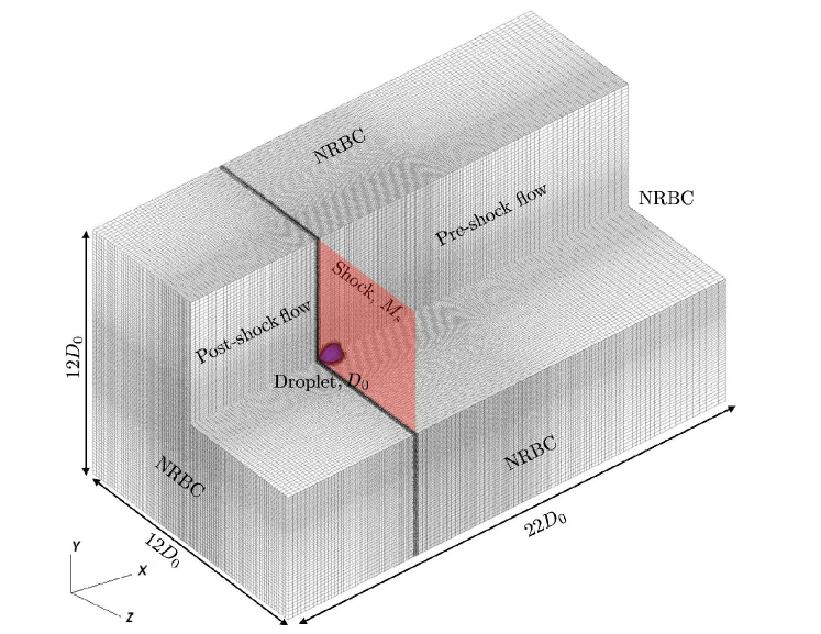
Figure 1: Initial computational mesh and set-up for the numerical simulation of aerobreakup.

2.1 Problem definition

Aerobreakup occurs when a liquid drop is suddenly exposed to a high-speed gas flow. These initial conditions are typically generated using a planar shock due to its simplicity, robustness and repeatability in both experiments and simulations without significantly interfering with the droplet or the evolution of the subsequent stages of the aerobreakup. In the simulation, we match the experimentally measured mean shock-strength $M_{s}\sim 1.3$, the Reynolds number ${\rm{Re}}=\frac{u_{s}D_{0}}{\nu}$ and the Weber number ${\rm{We}}=\frac{\rho_{g}u_{s}^{2}D_{0}}{\sigma}$, where $D_{0}$, $u_{s}$, $\nu$ and $\sigma$ denote the initial droplet diameter, the post-shock gas velocity, the kinematic viscosity of the gas as well as the surface-tension coefficient. In the experiments we mainly focus on the piercing regime with mean Weber numbers in the range of ${\rm{We}}=[200,700]$. Numerically, we conduct two simulations, where one matches a mean experimental Weber number of ${\rm{We}}\sim 470$ and one without any surface-tension effects, which is denoted in the following as ${\rm{We}}\to\infty$. Note that ${\rm{We}}\to\infty$ is purely nomenclature and does not indicate the limiting process to infinite Weber number. In both cases the Reynolds number is set to ${\rm{Re}}\sim 7000$. Hence, we numerically probe and compare both the piercing and the stripping regime.

The simulations are carried out in rectangular computational domain, which is given by $[-7D_{0},15D_{0}]\times[-6D_{0},6D_{0}]\times[-6D_{0},6D_{0}]$. The domain size was chosen based on sensitivity studies, which aim to both minimize the influence of the domain boundary conditions as well as the computational effort. Our results are in line with previous studies (Meng & Colonius, 2018). To capture the non-axisymmetric, three-dimensional modulation of the droplet and its surrounding flow field, we refrain from imposing any symmetries or simplifications and carry out full three-dimensional simulations for which the initial computational mesh and the set-up are shown in figure 1. The droplet is initially at rest and placed at the origin. On all domain boundaries, non-reflective boundary conditions (NRBC) are imposed. To ensure high spatial and temporal accuracy at reasonable computational costs, the adaptive mesh is composed out of four grid levels, which are adapted to follow the shocks, the interface and the turbulence. Therefore, as detailed and validated in Schmidmayer et al. (2019a), the refinement criterion reads

$$\frac{|X_{{\rm{Nb}}(i,j)}-X_{i}|}{\text{min}(X_{{\rm{Nb}}(i,j)}-X_{i})}>\varepsilon,$$ (20)

where $X$ indicates the flow variable for which we chose the density, velocity, pressure and volume fraction. The subscript Nb$(i,j)$ denotes the neighboring cells of cell $i$. The threshold is conservatively set to $\varepsilon=0.04$. As a result, the initial droplet is resolved by $D_{p}=140$ point per diameter, which was increased compared to Meng & Colonius (2018) in order to capture capillary effects such as the formation of ligaments during the course of the breakup. Note however, the selected resolution is by no means able to capture all fine-scale effects and the resolution required to do so will far exceed currently available computational resources, even on the largest of supercomputers (see, e.g., Meng & Colonius (2018) for estimates). However, as we will demonstrate below in section §4, the good agreement with the experiments gives us confidence that most pertinent effects of aerobreakup are indeed captured with the selected resolution. The mesh adaptivity, following both the droplet interface and the shock is exemplified by a snapshot in figure 2 during the initial phase of the simulation. In addition, a conservative grid stretching towards the domain boundaries as shown in figure 1 is used to further aid efficiency of the computations. Finally, to avoid spurious symmetries originating from the artificially symmetric initial conditions, we impose an initial velocity field with random perturbations of maximum $\mathcal{O}(10^{-4}u_{s})$. For the adaptive time marching scheme we maintain a maximum Courant-Friedrichs-Lewy (CFL) number of $0.3$.

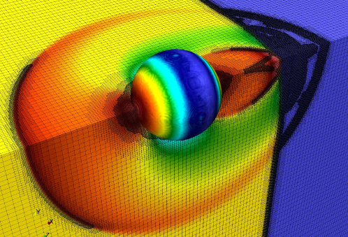
Figure 2: Snapshot of the adaptively refined mesh, colored by mixture pressure.

3 Experimental set-up

The shock tube is manufactured from several stainless steel pipes with shell thickness of $5~{}\mathrm{m}\mathrm{m}$ and circular cross-section of $52~{}\mathrm{m}\mathrm{m}$ in diameter. The facility consists of four components (Fig. 3): a driver section, a double-membrane section and a driven section which includes a test section of square cross-section of $46~{}\mathrm{m}\mathrm{m}$ $\times$ $46~{}\mathrm{m}\mathrm{m}$. Both membranes have the same burst pressure. The test section is connected on the driven section by means of circular-to-square transitions. Transitions are smooth and designed to preserve the area. The upstream transition is placed $1000~{}\mathrm{m}\mathrm{m}$ ahead from the center of the test section to insure a sharp and planar front wave profile. The test section is fitted with two oblong BK7 windows mounted opposite one another on its lateral sides to allow for optical diagnostics (shadowgraph or laser-sheet visualization). The double-membrane section and the driver section are pressurized with air at 75% and 125% of the burst pressure of the membranes (Mylar sheets), respectively. The shock wave is initiate by abruptly purging the double-membrane section through an extraction gas port. The driven section is filled with ambient air at controlled temperature.

To monitor the shock propagation, the instantaneous test section pressure is measured at four lateral positions by dynamic high-speed pressure transducers (noted C in Fig. 3) with acceleration compensation (Kistler 603B). They allow to measure pressure fluctuations over a range from vaccum to 200 bar with a rise time of 1  µ s . Each sensor is coupled to a Kistler 5018A charge amplifier (noted A in Fig. 3) with a bandwidth of 200  k Hz  which converts the mechanical stress into an electrical signal (0-10  V ). The electrical signal is acquired using a National Instruments NI PXIe-1073 module with 16 input channels with a frequency sample of 60 M Hz . The sensors have an active area of $5~{}\mathrm{m}\mathrm{m}$ diameter and are mounted in Pom-C ® holders. The active surface of the sensors is installed flush to the test section wall. These sensors are used to measure the shock wave velocity and the pressure jump, and are also exploited for the triggering of the high-speed camera. Synchronization of the high-speed camera with the light source emission and the breakup event is performed with a DG535 Digital Delay and Pulse Generator (Stanford Research system).

During the experiments, the water drop is held in a stable equilibrium at the center of the test section by the sound radiation pressure of an ultrasonic standing wave generated by the single-axis acoustic levitator. The levitator consists of a Langevin-type transducer coupled to a mechanical amplifier with a radiating surface of 35  m m  in diameter. The transducer operates at a resonant frequency of 20  k Hz  and is driven by a 1.5  k Hz  ultrasonic power supply. The radiating surface is mounted flush with the inside bottom surface of the chamber. Opposite to it, the upper surface of the chamber acts as a reflector of the acoustic waves for standing wave generation. To avoid disturbing the aerobreakup process with the sound radiation pressure, the levitation system is turned off following a voltage setpoint from a pressure transducer monitoring the shock propagation.

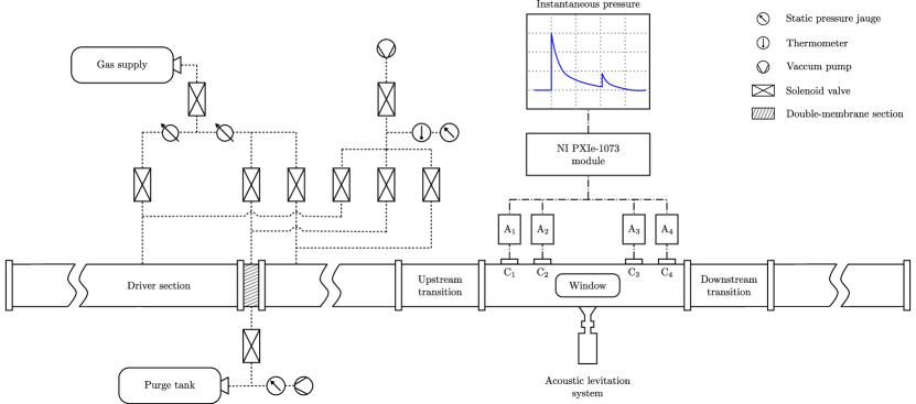
Figure 3: Shock tube facility (side view).

Aerobreakup experiments are captured with a high-magnification shadowgraphy system. The backlight illumination is provided by the laser-induced fluorescence of a Rhodamine 6G dye solution (Figure 4). A high-power dual oscillator/single head diode-pumped Nd:YAG laser (Mesa PIV, Continuum) delivering short pulses in the $120–180~{}\mathrm{n}\mathrm{s}$ range at repetition rate up to $80~{}\mathrm{k}\mathrm{Hz}$ is used to induce the fluorescence. Visualization is performed with a high-speed Fastcam Photron SA-Z equipped with a Maksutov–Cassegrain catadioptric microscope (QM1 Questar). The maximum optical resolution is 1.6  µ m  with a magnification up to 125:1. The depth of focus is approximately $0.6~{}\mathrm{m}\mathrm{m}$. The high-speed camera and the dual-cavity laser are synchronized by a digital delay generator. More details on the optical diagnostic are available in Biasiori-Poulanges & El-Rabii (2019). Sequence of images displayed are captured with camera settings adjusted to record frames at 512$\times$904 pixel resolution with a sampling frequency of $40~{}\mathrm{k}\mathrm{Hz}$. The average laser output power is $30~{}\mathrm{W}$ and the pulse width is $174~{}\mathrm{n}\mathrm{s}$. The measured spatial resolution of the imaging system was $6.5~{}\mathrm{\SIUnitSymbolMicro}\mathrm{m}$ per pixel. The time of the shock-wave interaction with the droplet ($t=0$) is determined by laser beam deflection with a continuous-wave laser beam perpendicular to the flow direction and tangent to the droplet front side. The deflection is recorded with a photodiode with a $0.9~{}\mathrm{n}\mathrm{s}$ risetime.

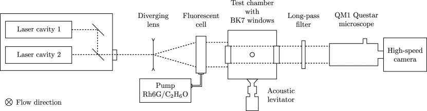
Figure 4: High-magnification shadowgraphy system (axial view).

4 Comparison of simulations and experiments

4.1 Droplet morphology

In order to compare the numerical simulation with images obtained from shadowgraphy in the following sections, we extract isosurfaces of volume fraction $\alpha_{l}=0.01$ from the simulation, and color them by velocity magnitude (see, also figures 5 and 7). Note that in diffuse interface methods, as employed here, the exact location of the interface is not well defined and it can only be approximated by isosurfaces of the volume fraction. While this leads to an ambiguous representation of the droplet surface, a sensitivity study in Meng & Colonius (2018) led to the conclusion that $\alpha_{l}=0.01$ was believed to be fair for comparison with experiments, considering the obscuring mist of the experiment, generated during the course of the breakup. For comparison of the numerical results with the experiment, we use, unless stated otherwise, the following non-dimensionalization

$$\bm{x}^{\ast}=\frac{\bm{x}}{D_{0}},\qquad\tau=t\frac{\bm{u}_{s}}{D_{0}}\sqrt{\frac{\rho_{s}}{\rho}},$$ (21)

where $\bm{x}$ and $t$ denote the dimensional location and time, respectively.

4.1.1 Finite Weber number case

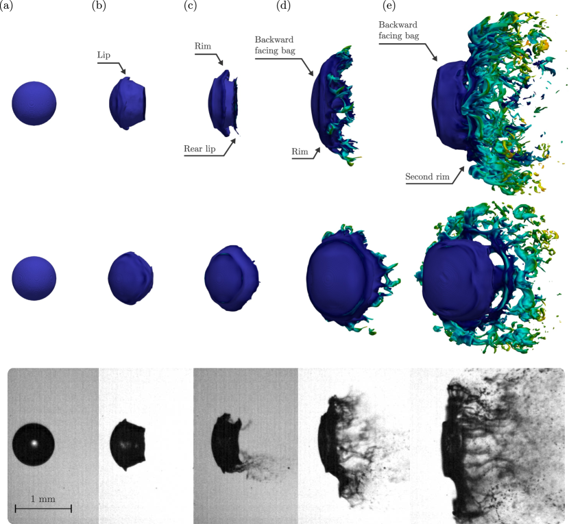
Figure 5: Numerical simulation of a water droplet aerobreakup (top two rows) and experimental visualizations (bottom rows). Characteristic times are (a) 0.00, (b) 0.27, (c) 0.47, (d) 0.72 and (e) 1.16. The timing information is for both experimental and numerical results expected for the numerical image (e) which corresponds to $\tau$=1.01. For the simulations, an isosurface of volume fraction $\alpha_{l}=0.01$ colored by velocity magnitude is depicted from two different perspectives. The scale bar refers to experimental results. The Weber number in the simulation and the experiment are 470 and 492, respectively.

At the first stages of the aerobreakup process ($\tau$ = 0.27 - 0.91), the numerical results show the typical droplet shapes that experimental visualizations (Figure 5) and literature report, with a good qualitative agreement with our experiment. First, the initial droplet deforms into a muffin-like shape, described by a spherical upstream side with lips growing in the spanwise direction. The droplet core takes the shape of a conic cylinder and the downstream side is flattened into a planar interface ($\tau$ = 0.27). While the droplet is continuously flattened, the stretching of lips in the streamwise direction results in a toroidal liquid rim ($\tau$ = 0.47). Simultaneously, rear lips raise in the downstream side. Owing to inertial forces, the rim at the droplet periphery is stretched, which deforms the droplet into a crescent-like shape ($\tau$ = 0.72). The rim begins to disintegrate into ligaments and subsequently into fragments. For characteristic times from 0.00 to 0.72, contours, extracted from the isosurfaces of the volume fraction $\alpha_{l}=0.01$ of the droplet, are overlaid on the experimental visualizations in figure 6. The contours are initially in good agreement with the experimental images. At later stages ($\tau$ = 0.72 - 1.16), the numerical results and the experimental visualizations both show a periodic distribution of ligaments, though there are discrepancies in the precise shape. However, the ligament distribution in the numerical simulation is consistent with the distribution experimentally observed as detailed below in section 5. Figure 5 shows that the toroidal rim is continuously sheared away with the flow for times $\tau$ = 0.72 - 1.16, which leads to a cylindrical curtain surrounding the droplet core and a cavity behind. This results in a backward facing bag. The downstream end of the bag bends in the spanwise direction forming a second rim, hindering the flow. Subsequently, the rim is subject to the development of multiple bags in the streamwise direction. Finally, bags are pierced by the flow, similar to bag and multimode breakup regimes. The ligaments resulting from this piercing process are tied up to their ends by the annular ring. The periodic nature of the ligament distribution is further discussed in section 5.1.

4.1.2 Simulation without surface tension

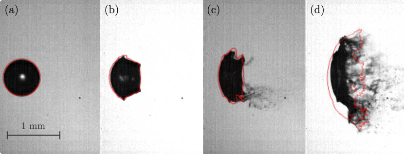
Figure 6: Overlaying of droplet contours from numerical results (red lines) on experimental images at the early stages of the aerobreakup. Characteristic times are (a) 0.00, (b) 0.27, (c) 0.47 and (d) 0.72. The Weber number in the simulation and the experiment are 470 and 492, respectively.

Next, in order to isolate the effect of surface tension during the breakup, we conduct an additional numerical simulation and set the surface tension to zero with $M_{s}$=1.3 and $D_{0}=0.804\mathrm{m}\mathrm{m}$ and compare the results with experiments at a high Weber number of ${\rm{We}}=1100$ ($M_{s}$=1.3, $d_{0}=1.68\mathrm{m}\mathrm{m}$).

Figure 7 shows that the droplet morphology and the mechanisms observed bear resemblance to the finite Weber number case, especially in the early stages. The droplet is first deformed into a muffin-like shape with lips growing in the spanwise direction. Lips are rapidly sheared away with the flow by forming a liquid rim surrounding the droplet body. The rim stretches in the streamwise direction and forms a cylindrical curtain, which eventually results in a backward facing bag. Finally and in contrast to the morphology previously observed in figure 5, much less distinct ligaments are formed and the liquid curtain breaks up directly into fine-scale structures due to a lack of the restoring surface tension forces.

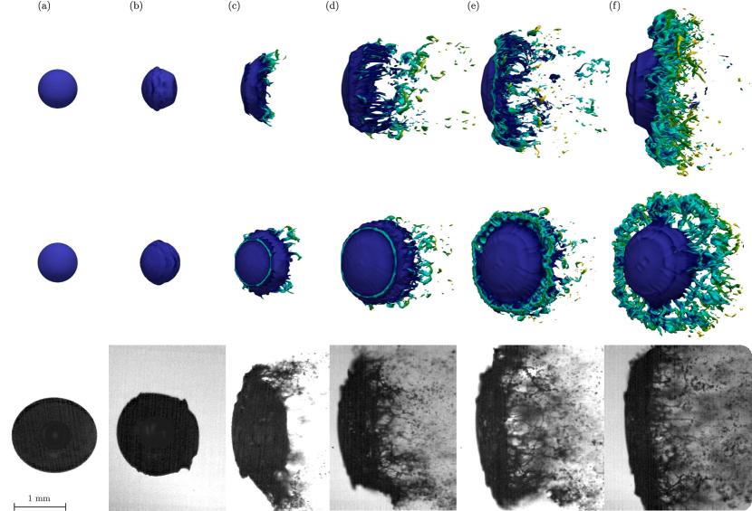
Figure 7: Numerical simulation of a water droplet aerobreakup and experimental visualizations. Characteristic times are (a) 0.00, (b) 0.20, (c) 0.52, (d) 0.73, (e) 0.86 and (f) 0.96. The scale bar refers to experimental results. In the experiment, the Weber numbers is ${\rm{We}}=1100$, whereas the simulation does not account for surface tension effects, i.e., ${\rm{We}}\to\infty$.

4.2 Center-of-mass evolution

Further validation is provided in figure 8 where the droplet center-of-mass drift from the numerical simulation is compared with that measured in the experiments. From the numerical simulation the center-of-mass is computed as in Meng & Colonius (2018) using:

$$\bm{x}_{c}=\frac{\int_{\Omega_{D}}\alpha_{l}\rho_{l}\bm{x}{\rm{dV}}}{\int_{\Omega_{D}}\alpha_{l}\rho_{l}{\rm{dV}}},$$ (22)

where $\Omega_{D}$ is the entire computational domain. On the experimental side, the evolution of the center-of-mass is computed from 2D-planar images, due to the line-integrated nature of images recorded by the shadowgraph. The center-of-mass is determined by calculating the first order spatial moment which is the intensity-weighted average of the pixel coordinates constituting the droplet. This requires a binary image. The binarization is performed by setting an intensity threshold to the image separating the droplet from the the background. Despite a slight deviation due to the 2D-planar assumption and the threshold sensitivity, figure 8 shows a good quantitative agreement between numerical results and the experiments. It can be noticed that the surface tension has no discernible affect on the drift in the simulations. This observation is consistent with the similar droplet morphology observed in both simulations at We=$470$ and ${\rm{We}}\to\infty$.

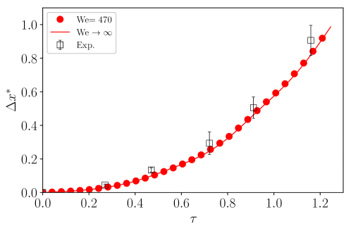
Figure 8: Evolution of the center-of-mass from numerical results and experimental observations. Error bars display the sensitivity of the center-of-mass detection to the intensity threshold used in the binarization process.

5 Formation of ligaments

For ${\rm{We}}>$10², the process of ligament formation is traditionally described by the sheet-thinning mechanism proposed by Liu & Reitz (1997) on the basis of the work of Stapper & Samuelsen (1990) for the breakup of a two-dimensional liquid sheet. Recently, the formation of ligaments has been re-evaluated (Jalaal & Mehravaran, 2014; Meng & Colonius, 2018) through 3D numerical simulations and an alternative driving mechanism has been proposed namely, the transverse azimuthal modulation. To date, no consensus has been found, and the ligament formation process has yet to be understood.

5.1 Ligament formation and azimuthal modulation

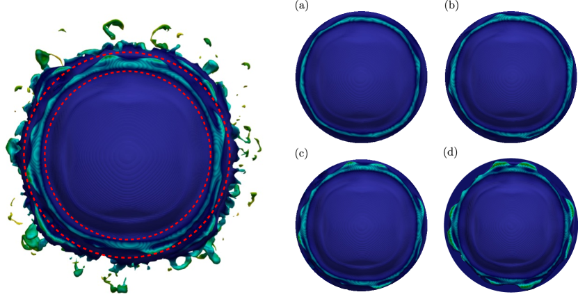
Figure 9: Transverse azimuthal modulation for ${\rm{We}}$=470 (front view). Characteristic times are (a) 0.79, (b) 0.82, (c) 0.84 and (d) 0.86. Images (a) to (d) are cropped views.

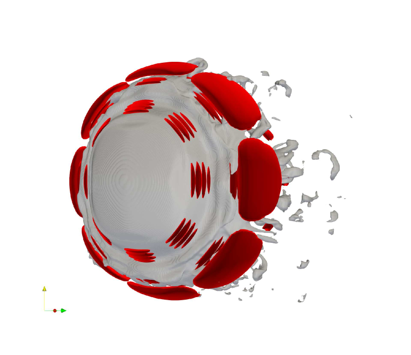
(a) m=4, $\tau\approx 0.85$

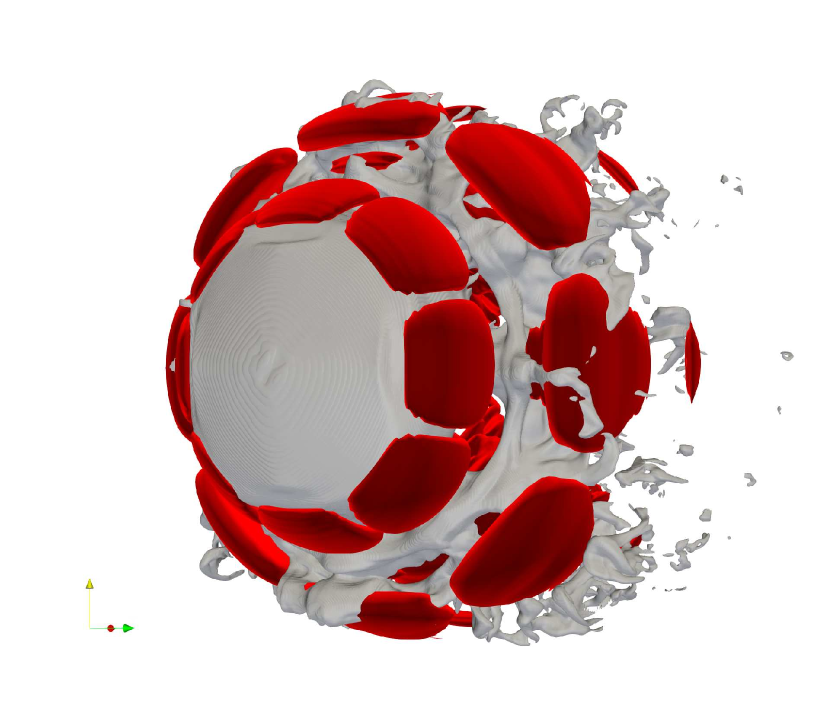
(b) m=4, $\tau\approx 0.97$

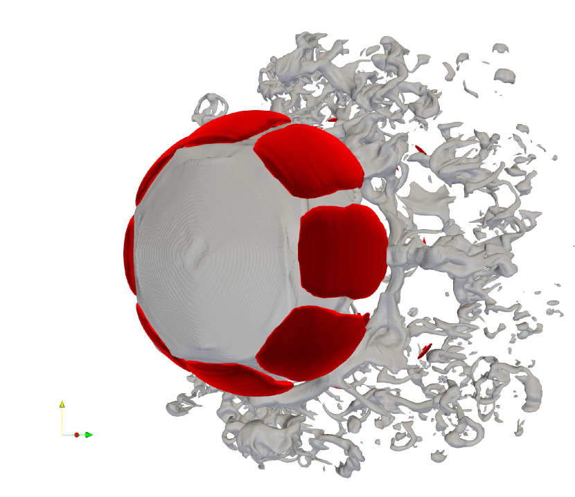
(c) m=4, $\tau\approx 1.05$

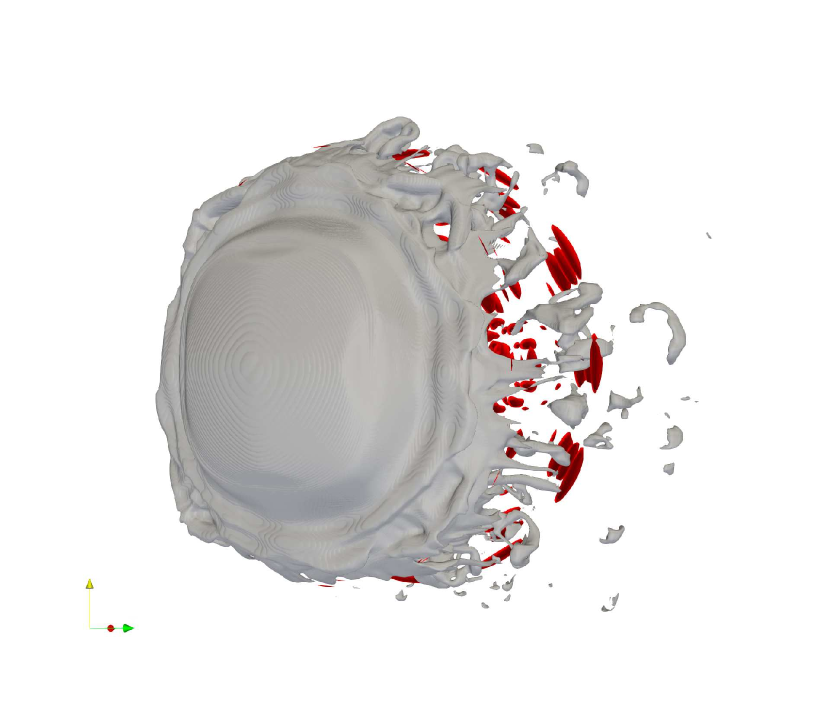
(d) m=6, $\tau\approx 0.85$

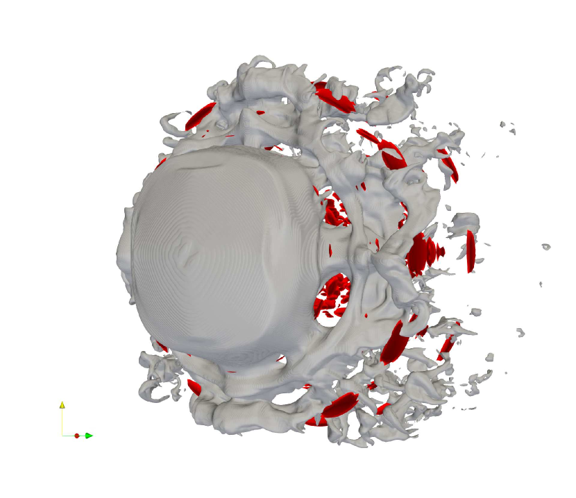
(e) m=6, $\tau\approx 0.97$

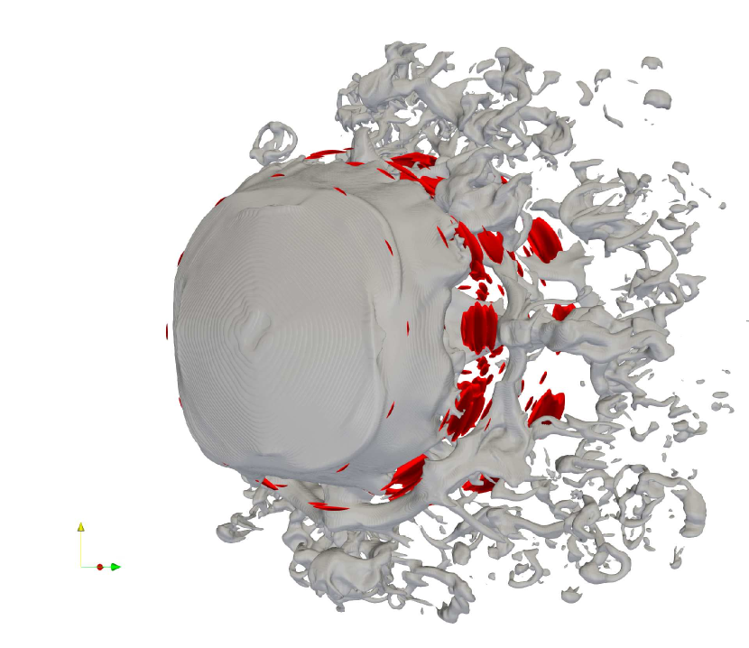
(f) m=6, $\tau\approx 1.05$

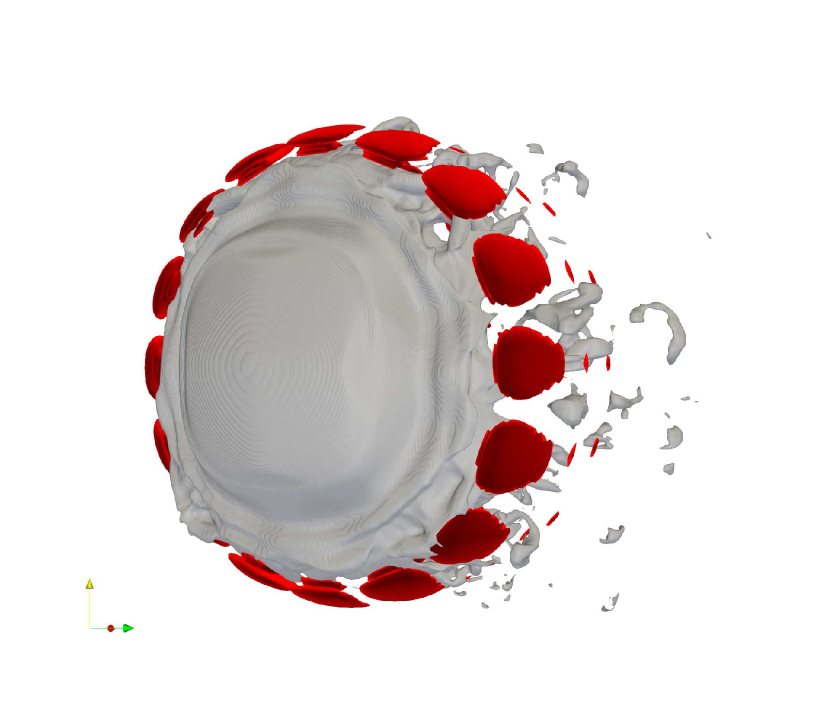
(g) m=8, $\tau\approx 0.85$

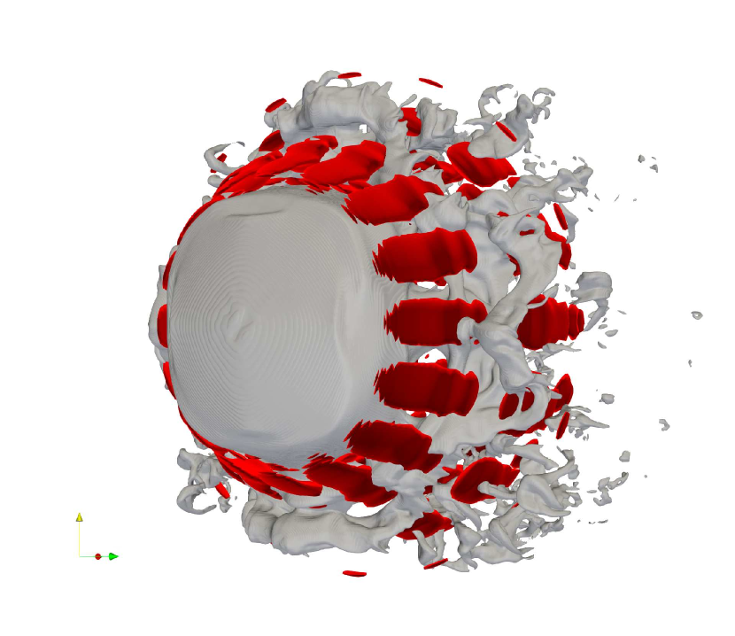
(h) m=8, $\tau\approx 0.97$

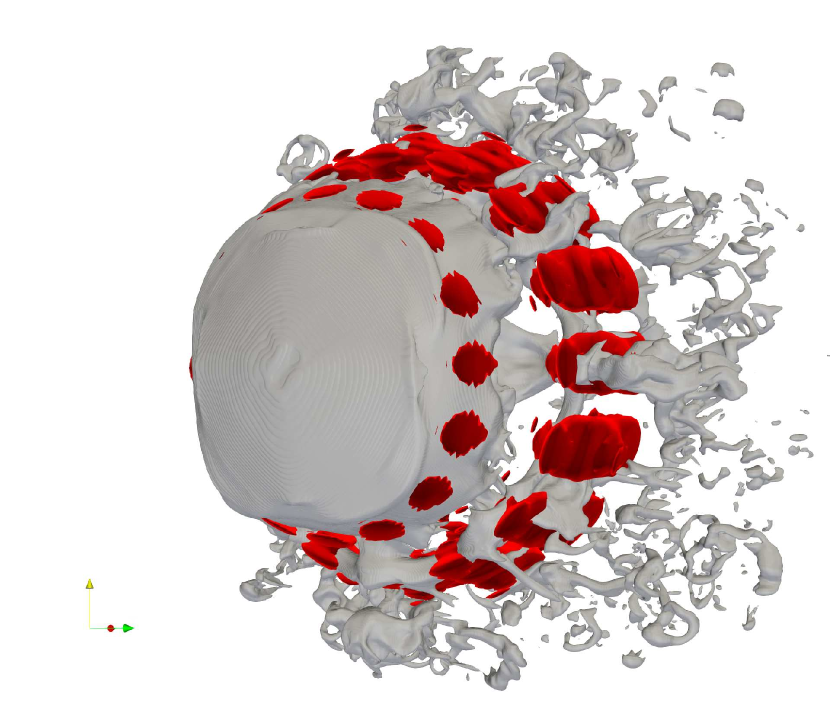
(i) m=8, $\tau\approx 1.05$

Figure 10: Isosurfaces of the $m$-th azimuthal mode $\kappa_{m}$ (red) and isosurfaces of the volume fraction $\alpha_{l}$=0.01 (grey) for ${\rm{We}}$=470.

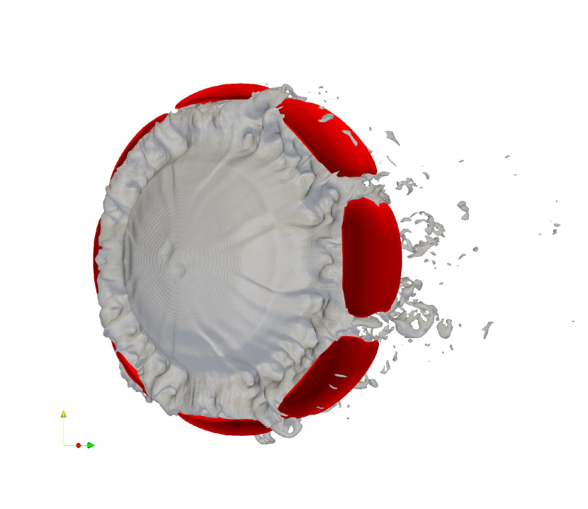
(a) m=4, $\tau\approx 0.85$

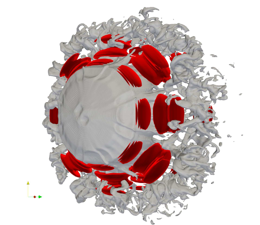
(b) m=4, $\tau\approx 0.97$

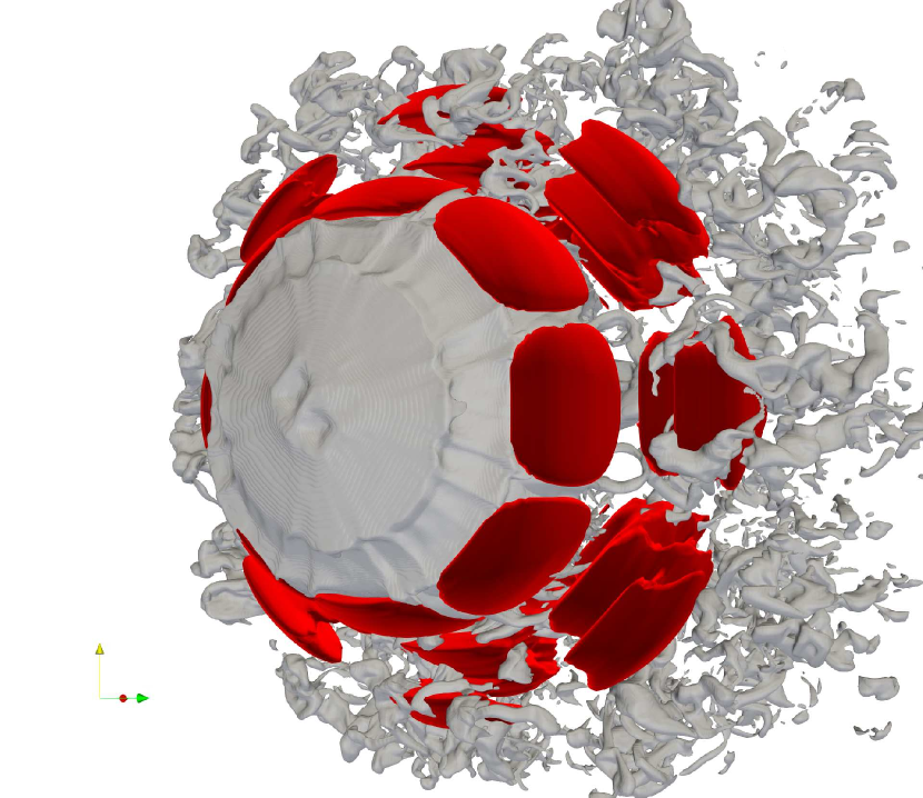
(c) m=4, $\tau\approx 1.05$

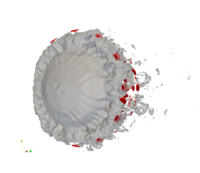
(d) m=6, $\tau\approx 0.85$

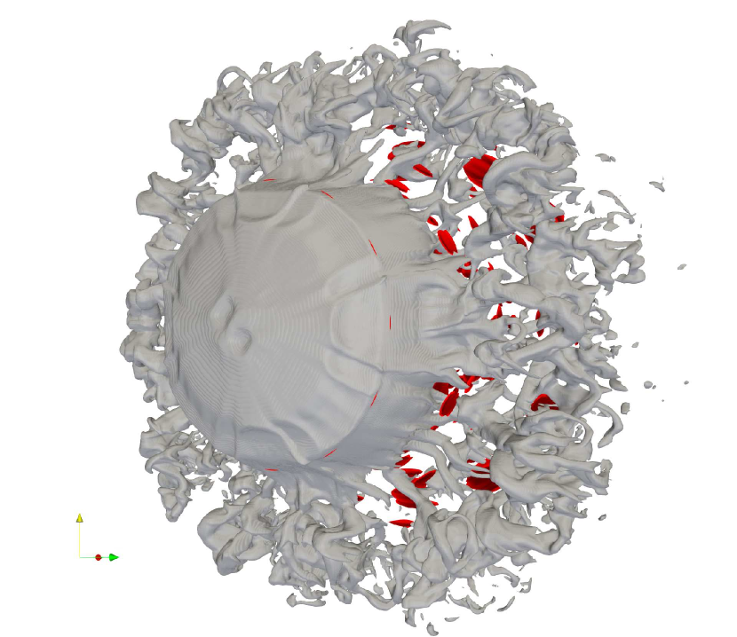
(e) m=6, $\tau\approx 0.97$

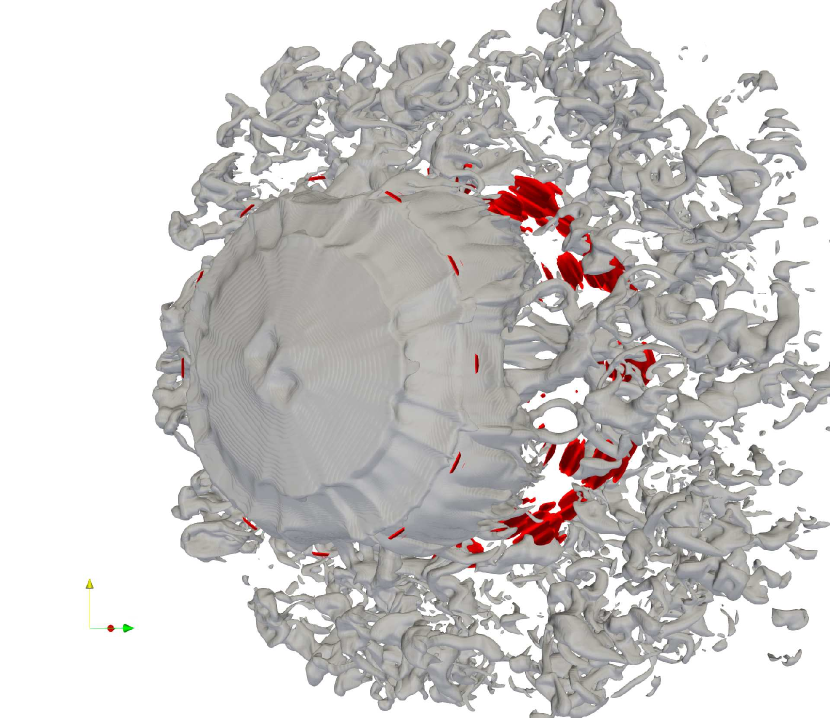
(f) m=6, $\tau\approx 1.05$

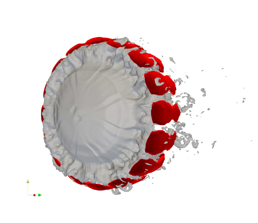
(g) m=8, $\tau\approx 0.85$

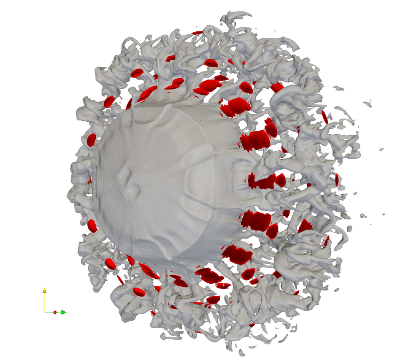
(h) m=8, $\tau\approx 0.97$

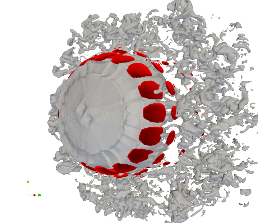
(i) m=8, $\tau\approx 1.05$

Figure 11: Isosurfaces of the $m$-th azimuthal mode $\kappa_{m}$ (red) and isosurfaces of the volume fraction $\alpha_{l}$=0.01 (grey) for ${\rm{We}}\to\infty$.

Exposing the water droplet to a high-speed gas flow can induce a large difference in the velocities between the two fluids and thus destabilize their interface. Depending on the flow conditions, the interface may be more susceptible to Rayleigh-Taylor or Kelvin-Helmholtz instabilities. The canonical Rayleigh-Taylor instability (RTI) occurs when a heavy fluid is suspended above a lighter fluid and both are subjected to acceleration. The interface begins to oscillate with alternating acceleration directions and is unstable when the acceleration is oriented towards the heavier fluid (Rayleigh, 1882). On the other hand, Kelvin-Helmholtz instability (KHI) arises due to either shear in a single fluid system or due to a velocity difference across the interface of two fluids, which results in propagating waves, and typically rollup into vortices, along the interface (Chandrasekhar, 1961).

For low Weber numbers (${\rm{We}}\sim$ 20), it is thought that the RTI is responsible for the bag-shape structure, which is attached to a thicker toroidal rim. Increasing the Weber number up to $80$, the standard bag morphology evolves to more complex bag-structures, namely the bag-and-stamen and multi-bag modes, still believed to be driven by RTI (Jain et al., 2015). Ultimately, bags undergo a piercing mechanism (Guildenbecher et al., 2009).

For higher Weber numbers there is less of a consensus but the markedly different droplet morphologies are also attributed to mechanisms other than RTI piercing. In the work of Jain et al. (2015) on the secondary atomization, the authors numerically investigate the shear-stripping regime, i.e., sheet-thinning regime, by running simulations at ${\rm{We}}$=120. Arguing that high inertial forces overcome the restoring effect of the surface tension, the authors state that the development of a potential bag on the rim is hampered by the stripping process occurring at the droplet equatorial plan. This indirectly exonerates the Rayleigh-Taylor piercing mechanism in the ligament formation. The authors suggest that the ligament formation owes to the high-speed gas flow over the droplet periphery, which results in transverse RTI. The crests of the transverse instability are deformed into ligaments by being stretched with the flow as described by Marmottant & Villermaux (2004). Following the work of Marmottant & Villermaux (2004) on the atomization of a liquid jet in coaxial flow, the recent work of Jalaal & Mehravaran (2014) suggests that axisymmetric waves, propagating on the droplet surface, are the result of KHI and that their acceleration leads to a transverse azimuthal modulation, which can be viewed as RTI. As a result of such KHI-RTI combination, streamwise ligaments are formed and subsequently fragmented into droplets. In addition, their 3D numerical simulations for Weber numbers up to 200 show a good qualitative agreement with their conjecture of an azimuthal modulation due to RTI. In a attempt to provide quantitative evidence, they compared the most-amplified wavenumbers, deduced from their simulations, with theoretical predictions but failed to find any conclusive quantitative agreement. In another attempt to find quantitative evidence of azimuthal RTI, Meng & Colonius (2018) performed a 3D simulation for ${\rm{We}}\to\infty$. In line with Jalaal & Mehravaran (2014), these simulations show a loss of axisymmetry, but a Fourier analysis of the velocity field reveals broadband instability growth for all modes and hence does not provide further evidence of transverse RTI.

In the present numerical simulations for ${\rm{We}}$ = 470, we also observe a loss of axisymmetry of the liquid sheet propagating on the droplet rim before transverse corrugations arise at the interface. In particular, as apparent from figure 9, we can see a non-uniform growth rate of the transverse corrugations, which results in variable crest amplitudes, indicating a transverse azimuthal modulation of the droplet. However, concerning the relation of the transverse instability with the ligament formation, a mismatch between the wavelength and the number of crests and ligaments does not seem to confirm the mechanism proposed by Jalaal & Mehravaran (2014). According to their conjecture, ligaments arise from the stretching of the interface corrugation crests due to aerodynamic forces. This implies that the number of ligaments is equal to the number of crests. As shown in figure 9, the number of crests observed in our simulation does not directly correspond to the eight ligaments, which are ultimately forming in the course of the breakup.

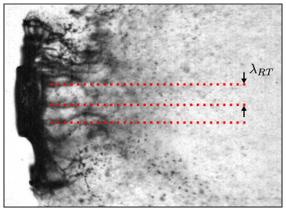
Figure 12: Measurement of ligament wavenumber.

For further investigation of the observed azimuthal modulation and to identify the modes which lead to the formation of the ligaments as well as to determine the effect of surface tension on these modes, we decompose the flow field around the droplet into azimuthal Fourier modes. To that end, the Cartesian mesh is interpolated onto a cylindrical mesh, where the resolutions in azimuthal direction $\theta$, radial direction $r$ and streamwise direction $x$ are kept similar to the Cartesian mesh. Subsequently, the azimuthal Fourier coefficients for each mode $\hat{\bm{u}}(x,r,t)$ are obtained by Fourier transforms in $\theta$ direction. We use an energy metric of the velocity for each mode, which is given by

$$\hat{\kappa}_{m}=|\hat{u}_{x,m}|^{2}+|\hat{u}_{r,m}|^{2}+|\hat{u}_{\theta,m}|^{2}.$$ (23)

Transforming $\hat{\kappa}_{m}$ back into physical space yields the azimuthal Fourier mode $\kappa_{m}$. Isosurfaces of selected azimuthal modes are superimposed with the isosurfaces of the volume fraction in figure 10, which shows that the azimuthal wavenumber $m=4$ and its harmonic $m=8$ are most pronounced on the droplet surface. Modes corresponding to wavenumbers other than $m=4$ or $m=8$, develop in the wake on the back of the droplet and do not appear to be responsible for the azimuthal modulation and deformation of the droplet itself. This is exemplarily shown for $m=6$ in figures 10(d)-10(f) but similarly observed for all other wavenumbers but $m=4$ and $m=8$. Strikingly, the wavenumbers $m=4$ and its harmonic $m=8$ do correspond to the wavenumber of the ligaments and thus directly relate the azimuthal modulation of the flow field to the formation of the ligaments.

Experimentally, we measure the mean wavenumber of the ligaments by manual post-processing of the shadowgraphs and measuring the distance between ligaments, where a ligament is defined as a coherent column of liquid as exemplified in figure 12. This procedure eventually yields a mean wavenumber of the ligaments of $m_{{\rm{exp}}}\sim 8.5$ , which is in excellent agreement with what is observed in our simulations. This further establishes validity of both our experiments and the numerical simulations.

When studying the evolution of the azimuthal structures of $m=4$ and $m=8$ in our numerical simulations, one can observe that these structures are formed at relatively early stages of the breakup and develop on the droplet surface. Subsequently, the azimuthal modes appear to deform the droplet surface, which leads to azimuthally distributed bag-like structures with wavenumber $m=8$. At later stages, these bag-like structures develop further and grow as they are subjected to the high-speed gas flow surrounding the droplet. Eventually, the aerodynamic forces are able to overcome the restoring effect of surface tension and pierce or rupture the bag-like structures, yielding ligaments, which, in first instance, remain attached to the circular rim before they detach at later stages. This piercing mechanism is illustrated by the detailed snapshots in figure 13, which show the evolution and rupture of the bag-like structures. It is also evident that eventually these ruptured pockets form the ligaments.

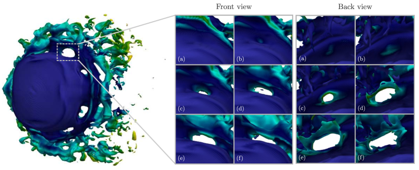
Figure 13: Piercing mechanisms for ${\rm{We}}$=470 (front and back views). Characteristic times are (a) 0.88, (b) 0.90, (c) 0.92, (d) 0.94, (e) 0.96 and (f) 0.98.

It is interesting to compare this picture to the We_σ=0 case, which is shown in figure 11. We can again observe that, as in the case of a finite Weber number, the only modes that are acting on the droplet surface correspond to the wavenumbers $m=4$ and $m=8$. This suggests that the cause and origin of these structure are independent of capillary effects. However, there are obvious differences in the subsequent evolution. In particular, it is apparent that the azimuthal disturbances are less amplified, and less able to modulate the cylindrical liquid curtain that is formed around the droplet core during the course of the breakup. Hence, in contrast to the finite Weber number case, there are no prominent bag-like structures, and the liquid curtain remains unruptured and intact, before it eventually disintegrates into fine-scale structures. This observation is also in good qualitative agreement with what was observed by others (Marmottant & Villermaux, 2004; Jalaal & Mehravaran, 2014) who conjecture that the transverse destabilisation of the liquid rim owes to the Rayleigh-Taylor instability, which leads to an infinitesimally small wavelength for negligible surface-tension values ($\sigma\to$ 0) as the RTI wavelength is proportional to the root of the surface tension.

While, we have not been able to infer a direct relation to RTI from our simulations, our observations do suggest that transverse azimuthal modulation plays a crucial role in the formation and subsequent shedding of ligaments.

5.2 Recurrent breakup and vortex shedding

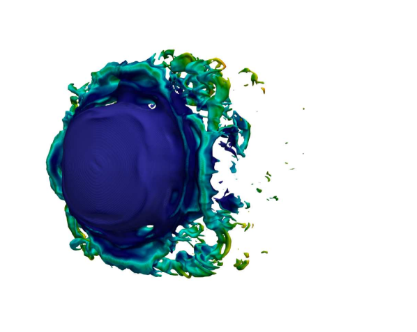
(a) Second breakup at $\tau=0.94$ for $\rm{We}=470$.

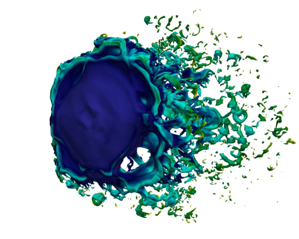
(b) Third breakup at $\tau=1.33$ for $\rm{We}=470$.

(c) Second breakup at $\tau=0.91$ for ${\rm{We}}\to\infty$.

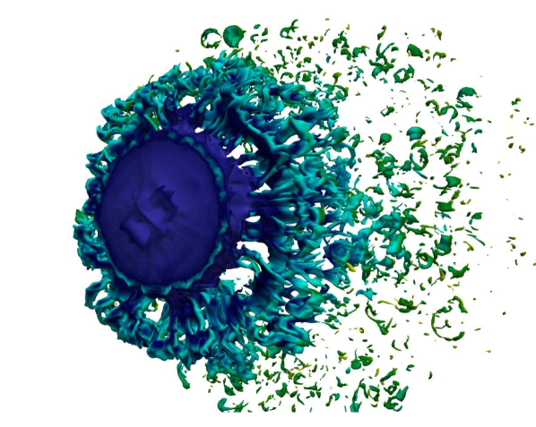
(d) Third breakup at $\tau=1.25$ for ${\rm{We}}\to\infty$.

Figure 14: Recurrent breakups for both simulations at $\rm{We}=470$ and ${\rm{We}}\to\infty$.

While the stages of the breakup and the formation of the ligaments are well described by the above mechanisms, our simulations and experiments suggest that the pattern of events occurs repeatably at different scale throughout the course of the breakup. In particular, when considering the breakup for a Weber number of $\rm{We}=470$ as shown in figures 14(a)-14(b), we can qualitatively observe a very similar droplet morphology and breakup behavior for times $\tau=0.94$ and $\tau=1.33$. Hence, the process repeats after the initial breakup or ligament formation process. An analogous process can also be observed in our simulations for ${\rm{We}}\to\infty$ as demonstrated in figures 14(d)-14(c), where the breakups are observed at $\tau=0.91$ and $\tau=1.25$. This suggests a negligible effect of capillary forces on such recurrent shedding behavior.

Consulting our experiments, we can investigate this effect for a longer time span than possible with the numerical simulations. To that end, the snapshots are post-processed manually and the breakup times are defined as the time between subsequent snapshots in which the ligaments are still attached to the main droplet core and when they have been shed from the droplet. This has been done for 29 independent experiments with varying Weber numbers. Starting from the formation of the first ligaments, we can observe a total of four breakups until the droplet is entirely disintegrated. A typical sequence of four breakups as captured by the experiments is shown in figure 15. Clearly visible are the ligaments and their subsequent fragmentation.

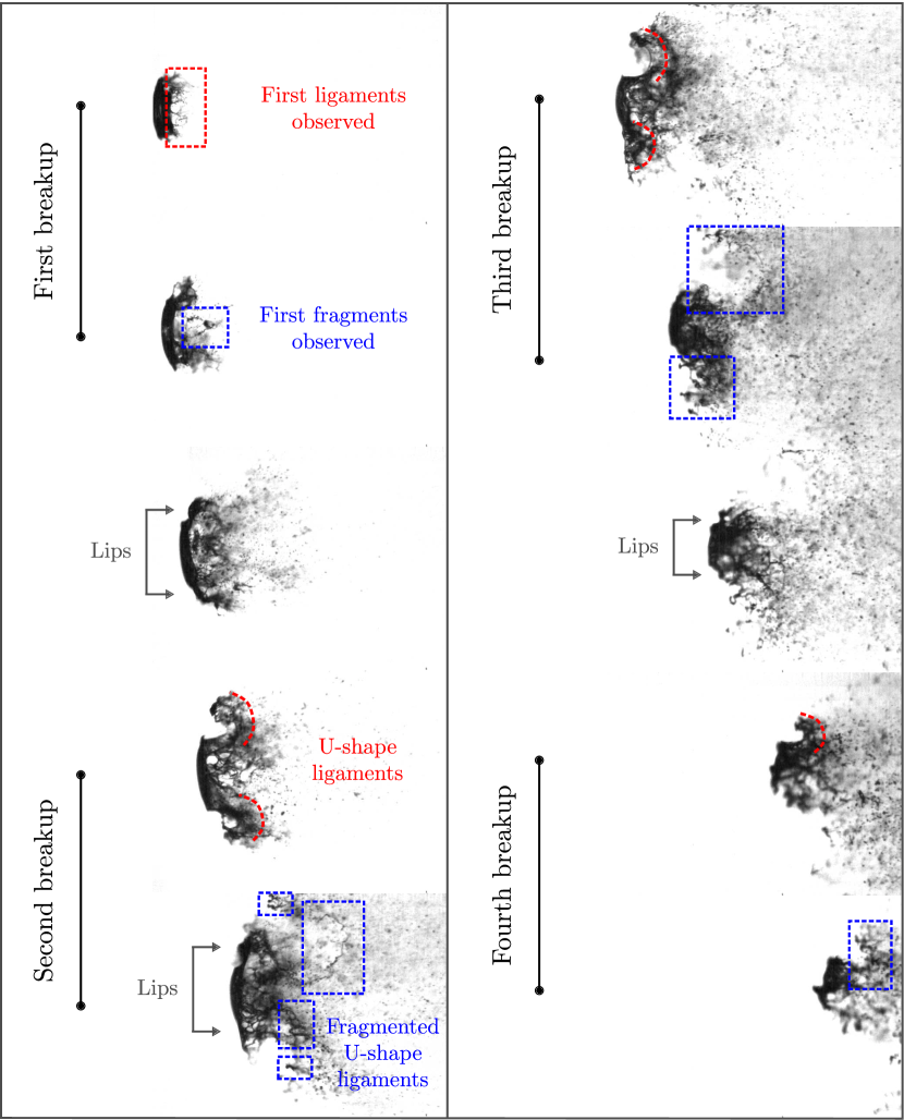
Figure 15: Experimental snapshots of the recurrent breakup mechanism for a typical case at $\rm{We}=295$.

Recording the breakup times as a function of the Weber number (figure 16) reveals that, while 4 breakups are recorded for all Weber numbers, capillary effects have an impact on the breakup times, reaching a nearly constant value beyond $We>400$. The error bars indicate the time difference between subsequent snapshots before and after the breakup of the ligaments. A comparison with our simulations in figure 16 shows that the first and second breakup times in the simulation agree well with the experimental observations for the second and third breakup for both the We=$470$ and ${\rm{We}}\to\infty$ simulations. This is believed to be due to the fine-scale nature of the first breakup, which our simulations are not able to resolve. Nonetheless, this further validates both the simulations as well as the post-processing methodology for the experiments.

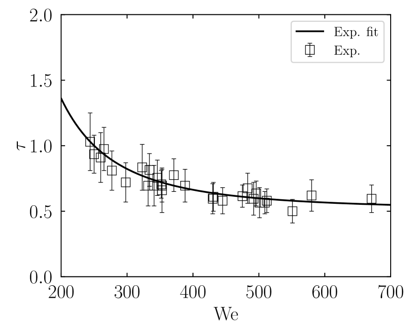
(a) First breakup.

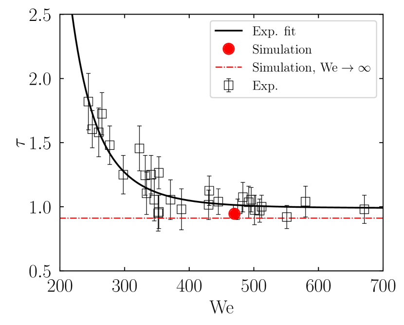
(b) Second breakup.

(c) Third breakup.

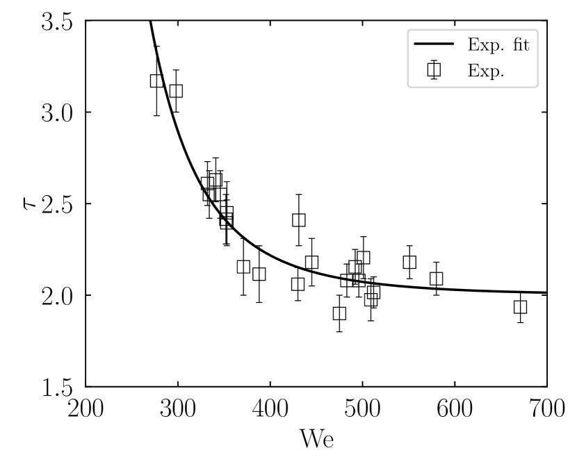
(d) Fourth breakup.

Figure 16: Breakup time dependence on the Weber number. The error bars indicate the time difference between subsequent snapshots before and after the breakup of the ligaments.

The functional dependence of the breakup onset to the Weber number is estimated using a nonlinear least-square fit of the experimental data of the form $\tau\approx a{\rm{We}}^{b}+c$ and plotted alongside the measurements in figure 16. The fitting coefficients are reported in table 1, which reveal a similar functional dependence for all breakup times. In particular, the similar exponents $a$ and constant difference between the offsets $c$ for all breakups reveal an approximately constant frequency between the breakups. This suggests that only the initial onset of the breakup is a function of the Weber number, whereas the breakup and its frequency are independent of capillary effects. Put differently, surface-tension seems to delay the onset of the initial ligament shedding but does not affect the frequency of the recurrent shedding. Hence, these curves can be collapsed when shifted by $c$, which is reported in figure 17. The fit suggests that the breakup onset scales with $\tau\sim{\rm{We}}^{-4}$.

Breakup No.	$a$	$b$	$c$
$1$	$4.07\cdot 10^{5}$	$-2.47$	$0.51$
$2$	$5.22\cdot 10^{12}$	$-5.36$	$0.99$
$3$	$8.58\cdot 10^{11}$	$-4.93$	$1.41$
$4$	$1.34\cdot 10^{12}$	$-4.92$	$2.00$
$all$	$5.41\cdot 10^{9}$	$-4.08$	$0$

Table 1: Fitting coefficients for a nonlinear least-square fit of the form $\tau\approx a{\rm{We}}^{b}+c$. The confidence interval for all fitting coefficients is 0.95.

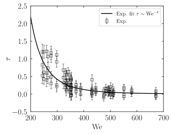
Figure 17: Collapse of all breakup times when shifted by their asymptotic breakup time. The least-square fit suggests $\tau\sim{\rm{We}}^{-4}$.

We conjecture that the breakup frequency is dominated by aerodynamical effects only. Such effects are dominant in the initial stages of the droplet deformation and previous studies of aerobreakup have shown a similar drag coefficient to that of a flow past a sphere (see, e.g., Meng & Colonius (2018)). In our case, it is instructive to evaluate the Strouhal number $St=\frac{fD}{U}$ for the observed breakups. However, the characteristic length-scale, associated to the deforming and disintegrating droplet and its wake, is a priori not clear.

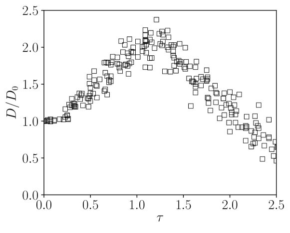
Figure 18: Diameter evolution for Weber numbers in the range $\rm{We}=[200,700]$.

To that end, in figure 18, we plot the evolution of the droplet core diameter throughout the breakup process for all experimental runs with Weber numbers in the range of $\rm{We}=[200,700]$. The diameter is measured directly from the shadowgraphs and defined as the maximum extent of the coherent liquid body of the droplet. Remarkably, the diameter evolution is independent of the Weber number and the droplet expands up to twice the size of its initial diameter for all experiments. Note that at later stages for $\tau>1$, the core diameter decreases due to shedding and $D<2D_{0}$ but the small-scale structures and mist shed form the droplet, yield an effective diameter which is larger than the diameter of the droplet core as plotted on figure 18. Hence, the maximum droplet diameter $D_{m}=2D_{0}$ as a characteristic length scale seems to be the natural choice for reduction of the breakup frequency. This yields a mean Strouhal number of $\rm{St}\approx 0.217$ when using all experimental data. Using the fitted data, one similarly obtains $\rm{St}\approx 0.18$. Both frequencies agree well with what is observed for the flow past a rigid sphere (see, e.g., Achenbach (1974); Kim & Durbin (1988); Sakamoto & Haniu (1990)). This suggests that the recurrent breakup is indeed induced by classical vortex shedding.

6 Conclusion

Three dimensional simulations and high-magnification shadowgraphy visualizations of the aerobreakup of a water droplet have been performed to capture the underlying mechanisms leading the ligament formation and disintegration. The numerical simulations are first validated with respect to experimental results by comparison of observed deformation and the evolution of the center of mass of the droplet, and the number of ligaments that are formed during breakup. An analysis of the perturbations arising on the liquid sheet surrounding the droplet shows good qualitative agreement with the concept of transverse azimuthal modulation. From the numerical results, modes associated with the transverse destabilization have been found by means of an azimuthal Fourier decomposition of the flow field. These correspond to the wavenumber of ligaments which form subsequent to the initial growth of azimuthal modulation. Finally, we experimentally and numerically show what we believe to be the first observation of recurrent shedding of ligaments. The first breakup event occurs at a time that depends weakly on the Weber number and with stronger capillarity the breakup is delayed, whereas subsequent events occur at the same fixed time interval, independent of We. The frequency of recurrence of breakup events is therefore driven primarily by inertia. By casting the frequency as a Strouhal number based on the pancaked droplet diameter, which reached a value of $2D_{0}$ compared to the initial droplet diameter, independent of We, we find $St\approx 0.2$, which supports a hypothesis that this shedding behavior is related to vortex shedding in the wake of the deformed droplet.

References

- Abgrall & Karni (2001) Abgrall, R. & Karni, S. 2001 Computations of compressible multifluids. Journal of computational physics 169 (2), 594–623.
- Achenbach (1974) Achenbach, E. 1974 Vortex shedding from spheres. Journal of Fluid Mechanics 62 (2), 209–221.
- Allison et al. (2016) Allison, P.M., McManus, T.A. & Sutton, J.A. 2016 Quantitative fuel vapor/air mixing imaging in droplet/gas regions of an evaporating spray flow using filtered rayleigh scattering. Optics letters 41 (6), 1074–1077.
- Ball et al. (2000) Ball, G.J., Howell, B.P., Leighton, T.G. & Schofield, M.J. 2000 Shock-induced collapse of a cylindrical air cavity in water: a free-lagrange simulation. Shock Waves 10 (4), 265–276.
- Biasiori-Poulanges & El-Rabii (2019) Biasiori-Poulanges, L. & El-Rabii, H. 2019 High-magnification shadowgraphy for the study of drop breakup in a high-speed gas flow. Optics letters 44 (23), 5884–5887.
- Bolleddula et al. (2010) Bolleddula, D.A., Berchielli, A. & Aliseda, A. 2010 Impact of a heterogeneous liquid droplet on a dry surface: Application to the pharmaceutical industry. Advances in colloid and interface science 159 (2), 144–159.
- Cao et al. (2007) Cao, X.K., Sun, Z.G., Li, W.F., Liu, H.F. & Yu, Z.H. 2007 A new breakup regime of liquid drops identified in a continuous and uniform air jet flow. Physics of Fluids 19 (5), 057103.
- Chandrasekhar (1961) Chandrasekhar, S. 1961 Hydrodynamic and hydromagnetic stability. Dover .
- Chen & Liang (2008) Chen, H. & Liang, S.M. 2008 Flow visualization of shock/water column interactions. Shock Waves 17 (5), 309–321.
- Chou et al. (1997) Chou, W.H., Hsiang, L.P. & Faeth, G.M. 1997 Temporal properties of drop breakup in the shear breakup regime. International Journal of Multiphase Flow 23 (4), 651–669.
- Cocchi & Saurel (1997) Cocchi, J.P. & Saurel, R. 1997 A riemann problem based method for the resolution of compressible multimaterial flows. Journal of Computational Physics 137 (2), 265–298.
- Coralic & Colonius (2014) Coralic, V. & Colonius, T. 2014 Finite-volume WENO scheme for viscous compressible multicomponent flows. Journal of Computational Physics 274, 95–121.
- Dorschner et al. (2019) Dorschner, B., Schmidmayer, K., Biasiori-Poulanges, L., El-Rabii, H. & Colonius, T. 2019 Shock-induced atomization of water droplets. Bulletin of the American Physical Society 64.
- Eckhoff (2016) Eckhoff, R.K. 2016 Explosion hazards in the process industries. Gulf Professional Publishing.
- Faeth et al. (1995) Faeth, G.M., Hsiang, L.P. & Wu, P.K. 1995 Structure and breakup properties of sprays. International Journal of Multiphase Flow 21, 99–127.
- Fishburn (1974) Fishburn, B.D. 1974 Boundary layer stripping of liquid drops fragmented by taylor instability. Acta Astronautica 1 (9-10), 1267–1284.
- Fuster (2018) Fuster, D. 2018 A review of models for bubble clusters in cavitating flows. Flow, Turbulence and Combustion pp. 1–40.
- Garrick (2016) Garrick, D.P. 2016 Numerical modeling of atomization in compressible flow. PhD thesis, Iowa State University.
- Gelfand (1996) Gelfand, B.E. 1996 Droplet breakup phenomena in flows with velocity lag. Progress in energy and combustion science 22 (3), 201–265.
- Gel’Fand et al. (1974) Gel’Fand, B.E., Gubin, S.A. & Kogarko, S.M. 1974 Various forms of drop fractionation in shock waves and their special characteristics. Journal of engineering physics 27 (1), 877–882.
- Guildenbecher et al. (2009) Guildenbecher, D.R., López-Rivera, C. & Sojka, P.E. 2009 Secondary atomization. Experiments in Fluids 46 (3), 371.
- Guildenbecher et al. (2011) Guildenbecher, DR, López-Rivera, C & Sojka, PE 2011 Droplet deformation and breakup. In Handbook of Atomization and Sprays, pp. 145–156. Springer.
- Han & Tryggvason (1999) Han, J. & Tryggvason, G. 1999 Secondary breakup of axisymmetric liquid drops. i. acceleration by a constant body force. Physics of fluids 11 (12), 3650–3667.
- Han & Tryggvason (2001) Han, J. & Tryggvason, G. 2001 Secondary breakup of axisymmetric liquid drops. II. Impulsive acceleration. Physics of Fluids 13 (6), 1554–1565.
- Hanson et al. (1963) Hanson, A.R., Domich, E.G. & Adams, H.S. 1963 Shock tube investigation of the breakup of drops by air blasts. The Physics of Fluids 6 (8), 1070–1080.
- Harper et al. (1972) Harper, E.Y., Grube, G.W. & Chang, I.D. 1972 On the breakup of accelerating liquid drops. Journal of Fluid Mechanics 52 (3), 565–591.
- Hinze (1955) Hinze, J.O. 1955 Fundamentals of the hydrodynamic mechanism of splitting in dispersion processes. AIChE Journal 1 (3), 289–295.
- Hirahara & Kawahashi (1992) Hirahara, H. & Kawahashi, M. 1992 Experimental investigation of viscous effects upon a breakup of droplets in high-speed air flow. Experiments in Fluids 13 (6), 423–428.
- Hsiang & Faeth (1992) Hsiang, L.P. & Faeth, G.M. 1992 Near-limit drop deformation and secondary breakup. International Journal of Multiphase Flow 18 (5), 635–652.
- Hsiang & Faeth (1993) Hsiang, L.P. & Faeth, G.M. 1993 Drop properties after secondary breakup. International Journal of Multiphase Flow 19 (5), 721–735.
- Hsiang & Faeth (1995) Hsiang, L.P. & Faeth, G.M. 1995 Drop deformation and breakup due to shock wave and steady disturbances. International Journal of Multiphase Flow 21 (4), 545–560.
- Hwang et al. (1996) Hwang, S.S., Liu, Z. & Reitz, R.D. 1996 Breakup mechanisms and drag coefficients of high-speed vaporizing liquid drops. Atomization and Sprays 6 (3).
- Jain et al. (2015) Jain, M., Prakash, R.S., Tomar, G. & Ravikrishna, R.V. 2015 Secondary breakup of a drop at moderate weber numbers. Proceedings of the Royal Society A: Mathematical, Physical and Engineering Sciences 471 (2177), 20140930.
- Jalaal & Mehravaran (2012) Jalaal, M. & Mehravaran, K. 2012 Fragmentation of falling liquid droplets in bag breakup mode. International Journal of Multiphase Flow 47, 115–132.
- Jalaal & Mehravaran (2014) Jalaal, M. & Mehravaran, K. 2014 Transient growth of droplet instabilities in a stream. Physics of Fluids 26 (1), 012101.
- Joseph et al. (1999) Joseph, D.D., Belanger, J. & Beavers, G.S. 1999 Breakup of a liquid drop suddenly exposed to a high-speed airstream. International Journal of Multiphase Flow 25 (6), 1263–1303.
- Kapila et al. (2001) Kapila, A., Menikoff, R., Bdzil, J., Son, S. & Stewart, D. 2001 Two-phase modeling of DDT in granular materials: Reduced equations. Physics of Fluids 13, 3002–3024.
- Khosla et al. (2006) Khosla, S., Smith, C.E. & Throckmorton, R.P. 2006 Detailed understanding of drop atomization by gas crossflow using the volume of fluid method. In 19th Annual Conference on Liquid Atomization and Spray Systems (ILASS-Americas), Toronto, Canada.
- Kim et al. (2006) Kim, D., Desjardins, O., Herrmann, M. & Moin, P. 2006 Toward two-phase simulation of the primary breakup of a round liquid jet by a coaxial flow of gas. Center for Turbulence Research Annual Research Briefs 185.
- Kim & Durbin (1988) Kim, H.J. & Durbin, P.A. 1988 Observations of the frequencies in a sphere wake and of drag increase by acoustic excitation. The Physics of fluids 31 (11), 3260–3265.
- Krzeczkowski (1980) Krzeczkowski, S.A. 1980 Measurement of liquid droplet disintegration mechanisms. International Journal of Multiphase Flow 6 (3), 227–239.
- Kulkarni & Sojka (2014) Kulkarni, V. & Sojka, P.E. 2014 Bag breakup of low viscosity drops in the presence of a continuous air jet. Physics of Fluids 26 (7), 072103.
- Lane (1951) Lane, W.R. 1951 Shatter of drops in streams of air. Industrial & Engineering Chemistry 43 (6), 1312–1317.
- Lee & Reitz (1999) Lee, C.H. & Reitz, R.D. 1999 Modeling the effects of gas density on the drop trajectory and breakup size of high-speed liquid drops. Atomization and Sprays 9 (5).
- Lee & Reitz (2000) Lee, C.H. & Reitz, R.D. 2000 An experimental study of the effect of gas density on the distortion and breakup mechanism of drops in high speed gas stream. International Journal of Multiphase Flow 26 (2), 229–244.
- Lee & Reitz (2001) Lee, C.S. & Reitz, R.D. 2001 Effect of liquid properties on the breakup mechanism of high-speed liquid drops. Atomization and Sprays 11 (1).
- Lefebvre & McDonell (2017) Lefebvre, A.H. & McDonell, V.G. 2017 Atomization and sprays. CRC press.
- Liu et al. (2019) Liu, N., Wang, Z., Sun, M., Deiterding, R. & Wang, H. 2019 Simulation of liquid jet primary breakup in a supersonic crossflow under adaptive mesh refinement framework. Aerospace Science and Technology 91, 456–473.
- Liu et al. (2018) Liu, N., Wang, Z., Sun, M., Wang, H. & Wang, B. 2018 Numerical simulation of liquid droplet breakup in supersonic flows. Acta Astronautica 145, 116–130.
- Liu et al. (2003) Liu, T.G., Khoo, B.C. & Yeo, K.S. 2003 Ghost fluid method for strong shock impacting on material interface. Journal of Computational Physics 190 (2), 651–681.
- Liu et al. (2011) Liu, W., Yuan, L. & Shu, C.W. 2011 A conservative modification to the ghost fluid method for compressible multiphase flows. Communications in Computational Physics 10 (4), 785–806.
- Liu & Reitz (1997) Liu, Z. & Reitz, R.D. 1997 An analysis of the distortion and breakup mechanisms of high speed liquid drops. International journal of multiphase flow 23 (4), 631–650.
- Magarvey & Taylor (1956) Magarvey, R.H. & Taylor, B.W. 1956 Free fall breakup of large drops. Journal of Applied Physics 27 (10), 1129–1135.
- Marcotte & Zaleski (2019) Marcotte, F. & Zaleski, S. 2019 Density contrast matters for drop fragmentation thresholds at low ohnesorge number. Physical Review Fluids 4 (10), 103604.
- Marmottant & Villermaux (2004) Marmottant, P. & Villermaux, E. 2004 On spray formation. Journal of fluid mechanics 498, 73–111.
- Meng (2016) Meng, J.C. 2016 Numerical simulations of droplet aerobreakup. PhD thesis, California Institute of Technology.
- Meng & Colonius (2014) Meng, J.C. & Colonius, T. 2014 Numerical simulations of the early stages of high-speed droplet breakup. Shock Waves pp. 1–16.
- Meng & Colonius (2018) Meng, J.C. & Colonius, T. 2018 Numerical simulation of the aerobreakup of a water droplet. Journal of Fluid Mechanics 835, 1108–1135.
- Pan et al. (2018) Pan, S., Han, L., Hu, X. & Adams, N. A. 2018 A conservative interface-interaction method for compressible multi-material flows. Journal of Computational Physics 371, 870–895.
- Pilch & Erdman (1987) Pilch, M. & Erdman, C.A. 1987 Use of breakup time data and velocity history to predict the maximum size of stable fragments for acceleration-induced breakup of a liquid drop. International Journal of Multiphase Flow pp. 13–6.
- Ranger & Nicholls (1969) Ranger, A.A. & Nicholls, J.A. 1969 Aerodynamic shattering of liquid drops. AIAA Journal 7 (2), 285–290.
- Rayleigh (1882) Rayleigh, L. 1882 Investigation of the Character of the Equilibrium of an Incompressible Heavy Fluid of Variable Density. Proceedings of the London Mathematical Society s1-14 (1), 170–177.
- Reinecke & Waldman (1975) Reinecke, W. & Waldman, G. 1975 Shock layer shattering of cloud drops in reentry flight. In 13th Aerospace Sciences Meeting, p. 152.
- Sakamoto & Haniu (1990) Sakamoto, H. & Haniu, H. 1990 A Study on Vortex Shedding From Spheres in a Uniform Flow. Journal of Fluids Engineering 112 (4), 386–392, arXiv: https://asmedigitalcollection.asme.org/fluidsengineering/article-pdf/112/4/386/5900198/386_1.pdf.
- Saurel et al. (2009) Saurel, R., Petitpas, F. & Berry, R.A. 2009 Simple and efficient relaxation methods for interfaces separating compressible fluids, cavitating flows and shocks in multiphase mixtures. Journal of Computational Physics 228(5), 1678–1712.
- Schmidmayer et al. (2019a) Schmidmayer, K., Petitpas, F. & Daniel, E. 2019a Adaptive Mesh Refinement algorithm based on dual trees for cells and faces for multiphase compressible flows. Journal of Computational Physics 388, 252–278.
- Schmidmayer et al. (2017) Schmidmayer, K., Petitpas, F., Daniel, E., Favrie, N. & Gavrilyuk, S.L. 2017 A model and numerical method for compressible flows with capillary effects. Journal of Computational Physics 334, 468–496.
- Schmidmayer et al. (2019b) Schmidmayer, K., Petitpas, F., Le Martelot, S. & Daniel, E. 2019b ECOGEN: An open-source tool for multiphase, compressible, multiphysics flows. Computer Physics Communications p. 107093.
- Shraiber et al. (1996) Shraiber, A.A., Podvysotsky, A.M. & Dubrovsky, V.V. 1996 Deformation and breakup of drops by aerodynamic forces. Atomization and Sprays 6 (6).
- Shyue & Xiao (2014) Shyue, K.M. & Xiao, F. 2014 An Eulerian interface sharpening algorithm for compressible two-phase flow: The algebraic THINC approach. Journal of Computational Physics 268, 326–354.
- Simpkins & Bales (1972) Simpkins, P.G. & Bales, E.L. 1972 Water-drop response to sudden accelerations. Journal of Fluid Mechanics 55 (04), 629–639.
- Stapper & Samuelsen (1990) Stapper, B.E. & Samuelsen, G.S. 1990 An experimental study of the breakup of a two-dimensional liquid sheet in the presence of co-flow air shear. In 28th Aerospace Sciences Meeting, p. 461.
- Theofanous (2011) Theofanous, T.G. 2011 Aerobreakup of newtonian and viscoelastic liquids. Annual Review of Fluid Mechanics 43, 661–690.
- Theofanous & Li (2008) Theofanous, T.G. & Li, G.J. 2008 On the physics of aerobreakup. Physics of Fluids 20 (5), 052103.
- Theofanous et al. (2004) Theofanous, T.G., Li, G.J. & Dinh, T.N. 2004 Aerobreakup in rarefied supersonic gas flows. J. Fluids Eng. 126 (4), 516–527.
- Toro (1997) Toro, E.F. 1997 Riemann solvers and numerical methods for fluid dynamics. Berlin: Springer Verlag.
- Van Leer (1977) Van Leer, B. 1977 Towards the ultimate conservative difference scheme III. Upstream-centered finite-difference schemes for ideal compressible flow. Journal of Computational Physics 23 (3), 263–275.
- Wadhwa et al. (2007) Wadhwa, A.R., Magi, V. & Abraham, J. 2007 Transient deformation and drag of decelerating drops in axisymmetric flows. Physics of Fluids 19 (11), 113301.
- Wang et al. (2014) Wang, C., Chang, S., Wu, H. & Xu, J. 2014 Modeling of drop breakup in the bag breakup regime. Applied Physics Letters 104 (15), 154107.
- Wierzba (1990) Wierzba, A. 1990 Deformation and breakup of liquid drops in a gas stream at nearly critical weber numbers. Experiments in fluids 9 (1-2), 59–64.
- Zhao et al. (2010) Zhao, H., Liu, H.F., Li, W.F. & Xu, J.L. 2010 Morphological classification of low viscosity drop bag breakup in a continuous air jet stream. Physics of Fluids 22 (11), 114103.
- Zhao et al. (2013) Zhao, H., Liu, H.F., Xu, J.L., Li, W.F. & Lin, K.F. 2013 Temporal properties of secondary drop breakup in the bag-stamen breakup regime. Physics of Fluids 25 (5), 054102.