Chemistry on quantum computers with virtual quantum subspace expansion

Abstract

Simulating chemical systems on quantum computers has been limited to a few electrons in a minimal basis. We demonstrate experimentally that the virtual quantum subspace expansion [Phys. Rev. X 10, 011004 (2020)] can achieve full basis accuracy for hydrogen and lithium dimers, comparable to simulations requiring twenty or more qubits. We developed an approach to minimize the impact of experimental noise on the stability of the generalized eigenvalue problem, a crucial component of the quantum algorithm. In addition, we were able to obtain an accurate potential energy curve for the nitrogen dimer in a quantum simulation on a classical computer.

It is expected that major applications of quantum computing will be in quantum chemistry ^{1, 2, 3}. Typical chemistry problems are to find the ground-state energy of a molecule, its excited states, or to extract reduced density matrices that can be used to compute various molecular properties relevant to science and industry. Traditional quantum algorithms, for example quantum phase estimation (QPE) ⁴, require circuit depths that are beyond the abilities of currently available quantum computers. A lot of effort has been invested into alternative approaches, most notably into the variational quantum eigensolver (VQE) algorithm ^{5, 6}. VQE is an iterative and hybrid quantum-classical method, where one creates a parametrized trial wave function on a quantum computer, measures observables that correspond to Hamiltonian terms of the studied molecule, estimates the electronic energy, and optimizes the set of wave-function parameters for the next iteration. It has been demonstrated that VQE can find the ground-state energy of small molecules ^{5, 7, 8, 9, 10, 11, 12, 13, 14}.

While the ground-state energy is an important property of a molecular configuration, the energy of excited states is even more important. The quantum subspace expansion (QSE) algorithm ¹⁵ can extract the energy of excited states described by the occupied and unoccupied orbitals in the active space and was also found to improve the ground-state energy estimate ^{16, 10}. Using this method, one first creates the ground-state wave function on a quantum computer and then performs extra measurements to analyze its single-particle or double-particle excitations. QSE does not require additional qubits or deeper circuits than VQE. Since this pioneering work, other extensions of VQE that target excited states within the active orbital space have been proposed and demonstrated ^{17, 18, 19}.

In most of the experimental realizations of molecular calculations on quantum computers, only small numbers of orbitals that constitute a subset of the basis of a many-electron wave function have been considered. While this is sometimes a reasonable approximation, not including additional virtual orbitals described by the chosen basis set limits the accuracy of molecular properties, for example reaction energetics and barriers, obtained with the algorithms discussed above. The number of orbitals accounted for in the simulation drives the number of qubits required and can quickly exceed those available on near-term quantum hardware. Circuit depths increase significantly with the number of orbitals used in the simulation as well. The virtual quantum subspace expansion (VQSE) algorithm, proposed in Ref. ²⁰, is an extension of QSE that includes excitations into virtual orbitals outside the chosen active space without the need for additional quantum resources. The authors analyzed VQSE in a numerical study and showed that it can improve accuracy of chemistry calculations. The algorithm assumes that strong correlations can be described by a subset of orbitals. Similarly to QSE, one creates the ground-state wave function using this subset on the quantum computer. VQSE then requires performing additional measurements to account for the so-called virtual orbitals that were not explicitly included in the determination of the ground-state energy, allowing one to estimate energy levels more accurately. VQSE scales polynomially with the size of the virtual orbital space. In principle, the other excited state approaches mentioned above could be adapted in a similar fashion to include additional virtual orbitals.

In this letter, we implement and execute the VQSE algorithm on a real quantum computer available on the IBM Q Hub and calculate the lowest-energy potential energy curves of the hydrogen, lithium, and nitrogen dimers. We find that the noise from the quantum computer significantly impacts the generalized eigenvalue problem that needs to be solved classically and develop and demonstrate an approach to overcome this issue. Our results show that VQSE works very well in experiments and even on imperfect and noisy devices.

VQSE proceeds in three steps. Firstly, we use a quantum computer to find the ground state in the active space. We do this using the VQE algorithm. Next, we measure expectation values of additional observables for the ground state. Finally, we use the measured expectation values to calculate corrections originating from the virtual space.

The electronic Hamiltonian is discretized into a finite set of orbitals. We divide the orbitals into core, active, and virtual orbitals. Core orbitals are considered frozen, i.e., these orbitals are doubly occupied and electrons in them are never excited into other orbitals. Since the Hamiltonian with frozen core orbitals can be transformed into a Hamiltonian with only active and virtual orbitals, we ignore the core space from now on. Active orbitals are the crucial part of the system because electrons in these orbitals are typically strongly correlated. Virtual orbitals give rise to corrections for quantities found by taking only the active orbitals into account.

We first create a set of expansions operators ²⁰,

$$S=\{a_{i}^{\dagger}a_{p},a_{\mu}^{\dagger}a_{q}a_{\nu}^{\dagger}a_{r}|i\in\mathcal{A}\cup\mathcal{V};p,q,r\in\mathcal{A};\mu,\nu\in\mathcal{V}\},$$ (1)

where $a^{\dagger}_{i}$ ($a_{i}$) is the creation (annihilation) operator for an electron in spin-orbital $i$, and $\mathcal{A}$ and $\mathcal{V}$ are sets of active-space and virtual-space spin-orbital indices, respectively. Let $\lvert\Psi\rangle$ be the ground-state wave function of a Hamiltonian $A$ restricted to the active space. States $O_{i}\lvert\Psi\rangle$, where $O_{i}\in S$, are single or double excitations of $\lvert\Psi\rangle$. We next create a matrix $A$ representing the unrestricted Hamiltonian in the expanded set of wave functions. $A$ is given by its elements

$$A_{ij}=\langle\Psi\rvert O_{i}HO_{j}\lvert\Psi\rangle,$$ (2)

where $O_{i},O_{j}\in S$. States $O_{i}\lvert\Psi\rangle$ are generally not orthonormal. To find the energy spectrum in the expanded set, it is thus necessary to solve a generalized eigenvalue problem

$$AC=BCE,$$ (3)

where the overlap matrix $B$ is given by its elements

$$B_{ij}=\langle\Psi\rvert O_{i}O_{j}\lvert\Psi\rangle,$$ (4)

$C$ is a matrix of eigenvectors, and $E$ is a diagonal matrix of eigenvalues.

The operators $O_{i}O_{j}$ and $O_{i}HO_{j}$ can be transformed using the Jordan–Wigner ²¹ or a similar transformation to qubit operators. If $\lvert\Psi\rangle$ is the ground-state wave function created on a quantum computer, the expectation values $\langle\Psi\rvert O_{i}O_{j}\lvert\Psi\rangle$ and $\langle\Psi\rvert O_{i}HO_{j}\lvert\Psi\rangle$ correspond to expectation values of strings of Pauli operators acting on qubits ²⁰.

We start with the simplest cases, finding the ground-state energy of the hydrogen and lithium dimers. We represent their electronic wave functions in the cc-pVDZ basis ²². The full molecular Hamiltonian of each molecule contains thousands of terms. We divide the Hilbert space of $\mathrm{H}_{2}$ into an active space with two orbitals and a virtual space with eight orbitals. Similarly, we divide the space of $\mathrm{Li}_{2}$ into a core space with two orbitals, an active space with two orbitals, and a virtual space with six orbitals.

Since our active spaces contain only two orbitals, they can be mapped to four qubits. We are targeting ground states with two electrons and zero total spin. This subspace contains only four basis states and can be mapped to two qubits ^{7, 10, 12}. We therefore reduce our four-qubit active-space Hamiltonian to a two-qubit Hamiltonian to further simplify the problem. We do this by projecting the Hamiltonian onto a subspace of wave functions that describe two electrons with opposite spins. The basis of this subspace is given by four-qubit states $\lvert 0011\rangle$, $\lvert 0110\rangle$, $\lvert 1001\rangle$, and $\lvert 1100\rangle$, where even and odd qubits represent spin-up and spin-down electrons, respectively. These four states are then mapped to the basis states of our two qubits. The projected Hamiltonian is given by

$$H=g_{1}I+g_{2}Z_{1}+g_{3}Z_{2}+g_{4}Z_{1}Z_{2}+g_{5}Y_{1}Y_{2},$$ (5)

where coefficients $g_{i}$ are calculated numerically. A transformation of the Hamiltonian to a smaller number of qubits is in principle possible also for larger systems. However, it is generally not scalable.

We use the VQE algorithm with the unitary coupled-clusters (UCC) ansatz ^{23, 24, 5, 7, 12} to find the ground state in the active space reduced to two qubits. The ansatz is given by

$$\lvert\psi(\theta)\rangle=e^{-i\theta Y_{1}X_{2}/2}\lvert\Phi\rangle,$$ (6)

where $Y_{1}$ and $X_{2}$ are Pauli Y and X matrices acting on the first and second qubit, respectively, and $\lvert\Phi\rangle=\lvert 00\rangle$ is the Hartree–Fock wave function. The wave function energy is given by

$$E(\theta)=g_{1}+g_{2}\langle Z_{1}\rangle_{\theta}+g_{3}\langle Z_{2}\rangle_{\theta}+g_{4}\langle Z_{1}Z_{2}\rangle_{\theta}+g_{5}\langle Y_{1}Y_{2}\rangle_{\theta},$$ (7)

where $\langle O\rangle_{\theta}=\langle\psi(\theta)\rvert O\lvert\psi(\theta)\rangle$. The ground state can be found by minimizing $E(\theta)$. Since ansatz (6) has one parameter only, we sweep the full domain of $\theta$ and perform the minimization during post-processing. We also measure other expectation values to estimate the elements of $A$ and $B$.

Energy levels of a molecule are the eigenvalues of the generalized eigenvalue problem (3). Elements of the $A$ and $B$ matrices are linear combinations of measured expectation values. They are noisy due to imperfections of real quantum computers and also due to shot noise. The noise perturbs the eigenvalue problem and results in nonphysical modes. As a result, the solutions to the generalized eigenvalue problem contain spurious states, also observed and discussed in the original QSE paper ¹⁰. A solution of the generalized eigenvalue problem exists only if $B$ is a positive-definite matrix. Both $A$ and $B$ are Hermitian indefinite matrices because they are created from noisy experimental data. The positive-definiteness of $B$ is therefore not guaranteed. To regularize the problem, we perform an eigenvalue decomposition of $B$, select an optimal number of largest eigenvalues, and project both $A$ and $B$ onto the subspace corresponding to these eigenvalues. We then solve the generalized eigenvalue problem with the projected matrices. The number of largest eigenvalues of $B$ that are preserved is maximized under the constraint that all of them are positive and that the projected generalized eigenvalue problem contains no spurious eigenvalues. The main problem is to decide if a particular eigenvalue is a regular eigenvalue or a spurious eigenvalue. We were not able to detect spurious eigenvalues by calculating the pseudospectra of the generalized eigenvalue problem since the ground state seems to be too sensitive to perturbations. Therefore, we detect spurious eigenvalues by computing finite differences of the lowest eigenvalue as a function of the number of preserved eigenvalues of $B$. We observe that the lowest eigenvalue decreases monotonically until either $B$ becomes indefinite or a spurious eigenvalue appears. The latter case results in a sudden jump in the energy. If we selected all positive eigenvalues instead of an optimized number of eigenvalues, spurious energy levels would appear in the obtained potential energy curves.

All calculations were performed on the IBM Q Johannesburg quantum computer. Since we used two qubits only, we estimated the overall circuit fidelity from reported gate fidelities for all pair of qubits and chose the pair with the highest overall fidelity. The selected qubits were qubits Q0 and Q1.

The executed circuit is shown in Fig. 1. It creates a UCC ansatz (6) and performs a measurement in a selected basis. Each $R_{t}$ gate is the $I$, $R_{x}(\pi/2)$, or $R_{y}(-\pi/2)$ gate for measuring the corresponding qubit in the $Z$, $Y$, or $X$ basis, respectively. Since the ansatz depends only on a single parameter, we do not perform the VQE feedback loop to find the energy minimum. We instead sample the full domain of $\theta$ and perform the minimization on a classical computer later. In particular, we run the circuit for 257 values of $\theta\in[-\pi,\pi]$ and for all nine combinations of the $R_{t}$ gates. Each individual circuit was sampled with 8192 shots. The raw data were unfolded ²⁵ to correct readout errors  ^{8, 11, 26}. We then calculated all two-qubits expectation values $\langle P_{1}P_{2}\rangle_{\theta}$, where $P_{i}\in\{I,X,Y,Z\}$ is a Pauli matrix acting on the $i$-th qubit. The same measured expectation values were used for both the $\mathrm{H}_{2}$ and $\mathrm{Li}_{2}$ molecules.

Figure 1: A quantum circuit for the preparation of the UCC ansatz (6) and for the measurement of its expectation values. Gates $R_{t}$ perform a basis transformation that depends on the measured term.

Next, we performed a separate calculation for each molecule and for each internuclear separation. The electronic wave functions were represented using the cc-pVDZ basis set. The Hamiltonian terms were calculated in OpenFermion ²⁷ using its interface to Psi4 ²⁸. The molecular Hamiltonian in the active space with two orbitals was transformed using the Jordan–Wigner transformation to a four-qubit Hamiltonian and then projected to a reduced two-qubit Hamiltonian. We then calculated and smoothed the expectation value of energy $E(\theta)$ from the measured expectation values and found $\theta_{\mathrm{min}}$ that minimized it. The minimal energy $E(\theta_{\mathrm{min}})$ is equivalent to the energy obtained using the VQE algorithm. All measured expectation values $\langle P_{1}P_{2}\rangle_{\theta}$ were evaluated at $\theta_{\mathrm{min}}$ for their use in later calculation stages.

We then created a list of expansion operators $O_{i}$. The operators that changed the total spin number or that produced a state with the norm below a cutoff when applied to the measured ground state were removed from the list. The $A$ matrix was calculated by first transforming operators $O_{i}HO_{j}$ using the Jordan–Wigner transformation to four-qubit operators and subsequently projecting them to two-qubit operators. The expectation value of each such two-qubit operator was then estimated from the evaluated expectation values $\langle P_{1}P_{2}\rangle_{\theta_{\mathrm{min}}}$. The $B$ matrix was created in a similar fashion.

Finally, we solved the generalized eigenvalue problem (3) to obtain the ground state energy. The solutions were sensitive to regularization because both matrices $A$ and $B$ were created from noisy data. We therefore first performed an eigenvalue decomposition of $B$, selected an optimal number of largest eigenvalues, and projected both $A$ and $B$ onto a subspace given by the eigenvectors corresponding to the selected eigenvalues. The generalized eigenvalue problem was solved using the projected $A$ and $B$ matrices. Fig. 2 shows the idea behind the regularization procedure. The lowest eigenvalue evolves in a continuous way for internuclear separations $R=1.0\,\text{\AA}$ and $R=1.1\,\text{\AA}$, although the number of positive eigenvalues of $B$ varies. For $R=1.2\,\text{\AA}$, a spurious eigenvalue appears from 166 eigenvalues onward. The optimum is therefore selected at 165 eigenvalues.

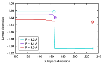
Figure 2: Results of the eigenvalue regularization procedure for the $\mathrm{H}_{2}$ molecule and three values of its internuclear separation $R$. The plot shows the lowest eigenvalue of generalized eigenvalue problem (3) as a function of the number of largest eigenvalues of the $B$ matrix preserved in the regularization procedure. Crosses mark energies obtained when preserving all positive eigenvalues. Circles mark energies found using our regularization method.

The calculations were performed both for zero virtual orbitals and the selected number of virtual orbitals. The results for zero virtual orbitals are equivalent to QSE results.

Potential energy curves for $\mathrm{H}_{2}$ in the ground state are shown in Fig. 3(a). The exact solutions were found by full configuration interaction (FCI) calculations within the chosen orbital subspace. Both VQE and QSE take into account the active space only. QSE substantially improved the VQE result. VQSE takes into account both the active and virtual spaces. Executing VQSE with two active and eight virtual orbitals gave rise to 296 expansion operators. VQSE significantly improved the accuracy of the ground state energy. Its results with eight virtual orbitals are close to the exact FCI result with ten virtual orbitals. The largest difference is $9.9\,\mathrm{mHa}$ at $R=0.9\,\text{\AA}$. The differences from the FCI solution are caused by noise. We confirmed this by executing VQSE with data obtained from a state-vector simulator. The noiseless result matched the FCI solution.

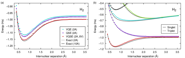
Figure 3: Potential energy curves of the $\mathrm{H}_{2}$ molecule. (a) Ground-state energy obtained using several methods. Numbers and letters in parentheses indicate the number of active (A) and virtual (V) orbitals. (b) Five lowest-energy states calculated using the VQSE algorithm with two active and eight virtual orbitals. Solid and dashed curves represent the exact solutions in the combined space.

Potential energy curves for $\mathrm{Li}_{2}$ in its singlet ground state are shown in Fig. 4(a). Similarly to $\mathrm{H}_{2}$, QSE improved the VQE result, but both methods take into account orbitals in the active space only. Solutions in the active space with two orbitals gave rise to an avoided crossing manifesting itself as a hump in the energy at intermediate internuclear separations. The hump is an artifact of a small active space and disappears when one takes additional orbitals into account. VQSE with two active and six virtual orbitals gave rise to 176 expansion operators. The VQSE method with two active and six virtual orbitals produced a result close to the exact FCI solution with eight active orbitals and without a hump. The largest difference is $2.5\,\mathrm{mHa}$ at $R=2.6\,\text{\AA}$. VQSE therefore improved the potential energy curve both qualitatively and quantitatively in this case.

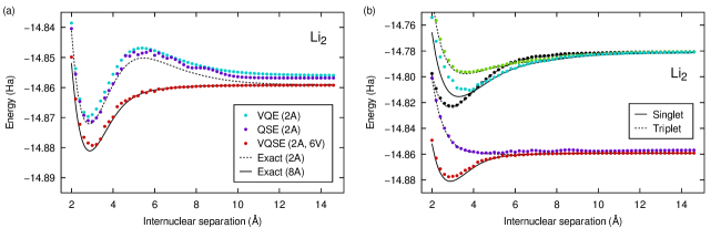
Figure 4: Potential energy curves of the $\mathrm{Li}_{2}$ molecule. (a) Singlet ground-state energy obtained using several methods. Numbers and letters in parentheses indicate the number of active (A) and virtual (V) orbitals. (b) Five lowest-energy states calculated using the VQSE algorithm with two active and six virtual orbitals. Solid and dashed curves represent the exact solutions in the combined space.

A useful property of VQSE is its ability to find energies of excited states. Lowest-energy states correspond to the smallest solutions of the generalized eigenvalue problem. Our implementation finds both singlet and triplet states due to the set of used expansion operators (1). The five lowest-energy states of both molecules are shown in Fig. 3(b) and Fig. 4(b). For regularizing the problem we did not use the same strategy as for the ground state since the excited states do not follow the monotonicity property of the ground state illustrated in Fig. 2. Instead, we removed spurious eigenvalues by preserving a constant number of the largest eigenvalues of the $B$ matrix for all data points. In particular, we preserved the 84 and 64 largest eigenvalues for $\mathrm{H}_{2}$ and $\mathrm{Li}_{2}$, respectively. These were the largest numbers of preserved eigenvalues that did not result in spurious energy levels.

There are only two electrons in the active and virtual spaces of both $\mathrm{H}_{2}$ and $\mathrm{Li}_{2}$ considered here. The combined spaces can be covered by single and double excitations of the Hartree–Fock states. VQSE therefore does not provide any advantage over configuration interaction with singles and doubles (CISD) for these problems. To show that VQSE can outperform CISD, we additionally calculated the energy of the nitrogen dimer. Since it is challenging to run this calculation on available quantum computers, we simulated the VQSE algorithm classically.

We considered $\mathrm{N}_{2}$ in the cc-pVDZ basis with four core orbitals, six active orbitals with six electrons, and three virtual orbitals. The UCC ansatz with singles and doubles (UCCSD) ^{23, 24} was used as the ansatz for the ground state in the active space. We included only excitation operators preserving the $z$-component of the total spin. The resulting ansatz had 117 parameters. We note that more compact ansatzes, such as ADAPT-VQE ²⁹, $k$-UpCCGSD ³⁰, sequences of Jastrow-type operators ³¹, or UCCSD variants ³² are possible but were not explored in this work. Both the Hamiltonian and the ansatz were transformed to the qubit space using the Jordan–Wigner transformation and the expectation value of the Hamiltonian was calculated numerically. The ansatz wavefunction was calculated exactly and without any approximations, such as the first-order Suzuki–Trotter approximation, that would be required to implement the ansatz on a quantum computer. The energy minimum was found using the L-BFGS-B algorithm ^{33, 34, 35}. We then directly calculated matrix elements of the $A$ and $B$ matrices from the optimized ansatz and used VQSE to find a correction to the ground-state energy. We compare the VQSE results with those of FCI and CISD calculations obtained from Psi4. The results are shown in Fig. 5. The UCCSD VQE in the six-orbital active space provides a significant improvement over CISD for this problem. With the inclusion of additional virtuals through the VQSE algorithm, we were able to obtain results that are close to the FCI results in nine orbitals. The simulation was exact, so instead of using our regularization procedure, we projected out space corresponding to eigenvalues of the $B$ matrix close to zero. The absence of spurious eigenvalues demonstrates that their source is indeed the noise from the quantum computer. The optimized state in the UCCSD form slightly differs from the exact ground state in the active space, which explains the remaining error. We emphasize that even in an ideal noiseless calculation presented here, the VQE algorithm could not obtain the exact ground state energy. The ansatz with single and double excitations is specified by a limited set of parameters and therefore does not cover the full active space. We also observed that the minimal energy depends significantly on the properties of the classical optimizer and on the initial guess of the ansatz parameters. We obtained the best results with all parameters being initially zero.

Even though current quantum computers have many qubits, it is still a major challenge to perform large-scale chemistry calculations on them. For example, the UCCSD circuits for the $\mathrm{N}_{2}$ molecule would require thousands of entangling quantum gates. The time required to execute each circuit would be far beyond the coherence times of existing qubits allowing for hundreds of gates at most. To our knowledge, the largest chemistry calculation performed to date on a quantum computer involved 12 qubits, 72 entangling gates, and 36 variational parameters ³⁶. The authors studied the Hartree–Fock state of a chain of 12 hydrogen atoms. Yet another bottleneck is the classical optimization loop in the VQE algorithm. Our classical simulation required 110,683 evaluations of the Hamiltonian expectation value. If one evaluation took one minute on a quantum computer, which is a very optimistic assumption, it would take months for the algorithm to converge. Furthermore, even ideal quantum computers produce statistical output containing shot noise. Classical optimizers are sensitive to noise, which requires careful selection of appropriate optimization algorithms and tuning their parameters ^{37, 38}. Overcoming these challenges will require major advances in quantum hardware and algorithms.

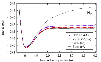
Figure 5: Potential energy curves of the $\mathrm{N}_{2}$ molecule in its ground state obtained using a classical simulation of the VQSE algorithm. Numbers and letters in parentheses indicate the number of active (A) and virtual (V) orbitals.

We implemented the VQSE method proposed in Ref. ²⁰ on the IBM Q Johannesburg quantum computer and used it to calculate the potential energy curves of the $\mathrm{H}_{2}$ and $\mathrm{Li}_{2}$ molecules. The noise of the quantum hardware is found to significantly impact the classical generalized eigenvalue problem and we developed a robust mathematical approach to address this issue. The obtained results show a significant improvement in accuracy over the VQE and QSE methods with the same number of qubits. In the present work, we used only two qubits to model molecules with up to ten orbitals, which would typically require twenty qubits using other algorithms. We also demonstrated the effectiveness of VQSE for larger problems by finding the ground-state potential energy curve of $\mathrm{N}_{2}$. VQSE is therefore a promising method for studying chemical systems on near-term quantum computers.

We thank Tyler Takeshita for helpful discussions. This work was supported by the DOE under contract DE-AC02-05CH11231, through the Office of Advanced Scientific Computing Research (ASCR) Quantum Algorithms Team and Accelerated Research in Quantum Computing programs. This research used resources of the Oak Ridge Leadership Computing Facility, which is a DOE Office of Science User Facility supported under Contract DE-AC05-00OR22725.

References

- Reiher et al. 2017 Reiher, M.; Wiebe, N.; Svore, K. M.; Wecker, D.; Troyer, M. Elucidating reaction mechanisms on quantum computers. Proc. Natl. Acad. Sci. U.S.A. 2017, 114, 7555–7560
- Cao et al. 2019 Cao, Y.; Romero, J.; Olson, J. P.; Degroote, M.; Johnson, P. D.; Kieferová, M.; Kivlichan, I. D.; Menke, T.; Peropadre, B.; Sawaya, N. P. D.; Sim, S.; Veis, L.; Aspuru-Guzik, A. Quantum Chemistry in the Age of Quantum Computing. Chem. Rev. 2019, 119, 10856–10915
- McArdle et al. 2020 McArdle, S.; Endo, S.; Aspuru-Guzik, A.; Benjamin, S. C.; Yuan, X. Quantum computational chemistry. Rev. Mod. Phys. 2020, 92, 015003
- Aspuru-Guzik et al. 2005 Aspuru-Guzik, A.; Dutoi, A. D.; Love, P. J.; Head-Gordon, M. Simulated Quantum Computation of Molecular Energies. Science 2005, 309, 1704–1707
- Peruzzo et al. 2014 Peruzzo, A.; McClean, J.; Shadbolt, P.; Yung, M.-H.; Zhou, X.-Q.; Love, P. J.; Aspuru-Guzik, A.; O’Brien, J. L. A variational eigenvalue solver on a photonic quantum processor. Nat. Commun. 2014, 5, 4213
- McClean et al. 2016 McClean, J. R.; Romero, J.; Babbush, R.; Aspuru-Guzik, A. The theory of variational hybrid quantum-classical algorithms. New J. Phys. 2016, 18, 023023
- O’Malley et al. 2016 O’Malley, P. J. J.; Babbush, R.; Kivlichan, I. D.; Romero, J.; McClean, J. R.; Barends, R.; Kelly, J.; Roushan, P.; Tranter, A.; Ding, N.; Campbell, B.; Chen, Y.; Chen, Z.; Chiaro, B.; Dunsworth, A.; Fowler, A. G.; Jeffrey, E.; Lucero, E.; Megrant, A.; Mutus, J. Y.; Neeley, M.; Neill, C.; Quintana, C.; Sank, D.; Vainsencher, A.; Wenner, J.; White, T. C.; Coveney, P. V.; Love, P. J.; Neven, H.; Aspuru-Guzik, A.; Martinis, J. M. Scalable Quantum Simulation of Molecular Energies. Phys. Rev. X 2016, 6, 031007
- Kandala et al. 2017 Kandala, A.; Mezzacapo, A.; Temme, K.; Takita, M.; Brink, M.; Chow, J. M.; Gambetta, J. M. Hardware-efficient variational quantum eigensolver for small molecules and quantum magnets. Nature 2017, 549, 242–246
- Shen et al. 2017 Shen, Y.; Zhang, X.; Zhang, S.; Zhang, J.-N.; Yung, M.-H.; Kim, K. Quantum implementation of the unitary coupled cluster for simulating molecular electronic structure. Phys. Rev. A 2017, 95, 020501
- Colless et al. 2018 Colless, J. I.; Ramasesh, V. V.; Dahlen, D.; Blok, M. S.; Kimchi-Schwartz, M. E.; McClean, J. R.; Carter, J.; de Jong, W. A.; Siddiqi, I. Computation of Molecular Spectra on a Quantum Processor with an Error-Resilient Algorithm. Phys. Rev. X 2018, 8, 011021
- Dumitrescu et al. 2018 Dumitrescu, E. F.; McCaskey, A. J.; Hagen, G.; Jansen, G. R.; Morris, T. D.; Papenbrock, T.; Pooser, R. C.; Dean, D. J.; Lougovski, P. Cloud Quantum Computing of an Atomic Nucleus. Phys. Rev. Lett. 2018, 120, 210501
- Hempel et al. 2018 Hempel, C.; Maier, C.; Romero, J.; McClean, J.; Monz, T.; Shen, H.; Jurcevic, P.; Lanyon, B. P.; Love, P.; Babbush, R.; Aspuru-Guzik, A.; Blatt, R.; Roos, C. F. Quantum Chemistry Calculations on a Trapped-Ion Quantum Simulator. Phys. Rev. X 2018, 8, 031022
- Ganzhorn et al. 2019 Ganzhorn, M.; Egger, D. J.; Barkoutsos, P.; Ollitrault, P.; Salis, G.; Moll, N.; Roth, M.; Fuhrer, A.; Mueller, P.; Woerner, S.; Tavernelli, I.; Filipp, S. Gate-Efficient Simulation of Molecular Eigenstates on a Quantum Computer. Phys. Rev. Appl. 2019, 11, 044092
- Kokail et al. 2019 Kokail, C.; Maier, C.; van Bijnen, R.; Brydges, T.; Joshi, M. K.; Jurcevic, P.; Muschik, C. A.; Silvi, P.; Blatt, R.; Roos, C. F.; Zoller, P. Self-verifying variational quantum simulation of lattice models. Nature 2019, 569, 355–360
- McClean et al. 2017 McClean, J. R.; Kimchi-Schwartz, M. E.; Carter, J.; de Jong, W. A. Hybrid quantum-classical hierarchy for mitigation of decoherence and determination of excited states. Phys. Rev. A 2017, 95, 042308
- Bonet-Monroig et al. 2018 Bonet-Monroig, X.; Sagastizabal, R.; Singh, M.; O’Brien, T. E. Low-cost error mitigation by symmetry verification. Phys. Rev. A 2018, 98, 062339
- Santagati et al. 2018 Santagati, R.; Wang, J.; Gentile, A. A.; Paesani, S.; Wiebe, N.; McClean, J. R.; Morley-Short, S.; Shadbolt, P. J.; Bonneau, D.; Silverstone, J. W.; Tew, D. P.; Zhou, X.; O’Brien, J. L.; Thompson, M. G. Witnessing eigenstates for quantum simulation of Hamiltonian spectra. Sci. Adv. 2018, 4, eaap9646
- 18 Ollitrault, P. J.; Kandala, A.; Chen, C.-F.; Barkoutsos, P. K.; Mezzacapo, A.; Pistoia, M.; Sheldon, S.; Woerner, S.; Gambetta, J.; Tavernelli, I. Quantum equation of motion for computing molecular excitation energies on a noisy quantum processor. arXiv:1910.12890 [quant-ph]
- Parrish et al. 2019 Parrish, R. M.; Hohenstein, E. G.; McMahon, P. L.; Martínez, T. J. Quantum Computation of Electronic Transitions Using a Variational Quantum Eigensolver. Phys. Rev. Lett. 2019, 122, 230401
- Takeshita et al. 2020 Takeshita, T.; Rubin, N. C.; Jiang, Z.; Lee, E.; Babbush, R.; McClean, J. R. Increasing the Representation Accuracy of Quantum Simulations of Chemistry without Extra Quantum Resources. Phys. Rev. X 2020, 10, 011004
- Jordan and Wigner 1928 Jordan, P.; Wigner, E. Über das Paulische Äquivalenzverbot. Z. Phys. 1928, 47, 631–651
- Dunning 1989 Dunning, T. H. Gaussian basis sets for use in correlated molecular calculations. I. The atoms boron through neon and hydrogen. J. Chem. Phys. 1989, 90, 1007–1023
- Bartlett et al. 1989 Bartlett, R. J.; Kucharski, S. A.; Noga, J. Alternative coupled-cluster ansätze II. The unitary coupled-cluster method. Chem. Phys. Lett. 1989, 155, 133–140
- Taube and Bartlett 2006 Taube, A. G.; Bartlett, R. J. New perspectives on unitary coupled-cluster theory. Int. J. Quantum Chem. 2006, 106, 3393–3401
- 25 Nachman, B.; Urbanek, M.; de Jong, W. A.; Bauer, C. W. Unfolding Quantum Computer Readout Noise. arXiv:1910.01969 [quant-ph]
- Yeter-Aydeniz et al. 2019 Yeter-Aydeniz, K.; Dumitrescu, E. F.; McCaskey, A. J.; Bennink, R. S.; Pooser, R. C.; Siopsis, G. Scalar quantum field theories as a benchmark for near-term quantum computers. Phys. Rev. A 2019, 99, 032306
- McClean et al. 2020 McClean, J. R.; Rubin, N. C.; Sung, K. J.; Kivlichan, I. D.; Bonet-Monroig, X.; Cao, Y.; Dai, C.; Fried, E. S.; Gidney, C.; Gimby, B.; Gokhale, P.; Häner, T.; Hardikar, T.; Havlíček, V.; Higgott, O.; Huang, C.; Izaac, J.; Jiang, Z.; Liu, X.; McArdle, S.; Neeley, M.; O’Brien, T.; O’Gorman, B.; Ozfidan, I.; Radin, M. D.; Romero, J.; Sawaya, N. P. D.; Senjean, B.; Setia, K.; Sim, S.; Steiger, D. S.; Steudtner, M.; Sun, Q.; Sun, W.; Wang, D.; Zhang, F.; Babbush, R. OpenFermion: The electronic structure package for quantum computers. Quantum Sci. Technol. 2020, 5, 034014
- Parrish et al. 2017 Parrish, R. M.; Burns, L. A.; Smith, D. G. A.; Simmonett, A. C.; DePrince, A. E.; Hohenstein, E. G.; Bozkaya, U.; Sokolov, A. Y.; Di Remigio, R.; Richard, R. M.; Gonthier, J. F.; James, A. M.; McAlexander, H. R.; Kumar, A.; Saitow, M.; Wang, X.; Pritchard, B. P.; Verma, P.; Schaefer, H. F.; Patkowski, K.; King, R. A.; Valeev, E. F.; Evangelista, F. A.; Turney, J. M.; Crawford, T. D.; Sherrill, C. D. Psi4 1.1: An Open-Source Electronic Structure Program Emphasizing Automation, Advanced Libraries, and Interoperability. J. Chem. Theory Comput. 2017, 13, 3185–3197
- Grimsley et al. 2019 Grimsley, H. R.; Economou, S. E.; Barnes, E.; Mayhall, N. J. An adaptive variational algorithm for exact molecular simulations on a quantum computer. Nat. Commun. 2019, 10, 3007
- Lee et al. 2019 Lee, J.; Huggins, W. J.; Head-Gordon, M.; Whaley, K. B. Generalized Unitary Coupled Cluster Wave functions for Quantum Computation. J. Chem. Theory Comput. 2019, 15, 311–324
- Matsuzawa and Kurashige 2020 Matsuzawa, Y.; Kurashige, Y. Jastrow-type Decomposition in Quantum Chemistry for Low-Depth Quantum Circuits. J. Chem. Theory Comput. 2020, 16, 944–952
- Sokolov et al. 2020 Sokolov, I. O.; Barkoutsos, P. K.; Ollitrault, P. J.; Greenberg, D.; Rice, J.; Pistoia, M.; Tavernelli, I. Quantum orbital-optimized unitary coupled cluster methods in the strongly correlated regime: Can quantum algorithms outperform their classical equivalents? J. Chem. Phys. 2020, 152, 124107
- Byrd et al. 1995 Byrd, R. H.; Lu, P.; Nocedal, J.; Zhu, C. A Limited Memory Algorithm for Bound Constrained Optimization. SIAM J. Sci. Comput. 1995, 16, 1190–1208
- Zhu et al. 1997 Zhu, C.; Byrd, R. H.; Lu, P.; Nocedal, J. Algorithm 778: L-BFGS-B: Fortran Subroutines for Large-Scale Bound-Constrained Optimization. ACM Trans. Math. Softw. 1997, 23, 550–560
- Morales and Nocedal 2011 Morales, J. L.; Nocedal, J. Remark on “Algorithm 778: L-BFGS-B: Fortran Subroutines for Large-Scale Bound Constrained Optimization”. ACM Trans. Math. Softw. 2011, 38
- 36 Arute, F.; Arya, K.; Babbush, R.; Bacon, D.; Bardin, J. C.; Barends, R.; Boixo, S.; Broughton, M.; Buckley, B. B.; Buell, D. A.; Burkett, B.; Bushnell, N.; Chen, Y.; Chen, Z.; Chiaro, B.; Collins, R.; Courtney, W.; Demura, S.; Dunsworth, A.; Farhi, E.; Fowler, A.; Foxen, B.; Gidney, C.; Giustina, M.; Graff, R.; Habegger, S.; Harrigan, M. P.; Ho, A.; Hong, S.; Huang, T.; Huggins, W. J.; Ioffe, L.; Isakov, S. V.; Jeffrey, E.; Jiang, Z.; Jones, C.; Kafri, D.; Kechedzhi, K.; Kelly, J.; Kim, S.; Klimov, P. V.; Korotkov, A.; Kostritsa, F.; Landhuis, D.; Laptev, P.; Lindmark, M.; Lucero, E.; Martin, O.; Martinis, J. M.; McClean, J. R.; McEwen, M.; Megrant, A.; Mi, X.; Mohseni, M.; Mruczkiewicz, W.; Mutus, J.; Naaman, O.; Neeley, M.; Neill, C.; Neven, H.; Niu, M. Y.; O’Brien, T. E.; Ostby, E.; Petukhov, A.; Putterman, H.; Quintana, C.; Roushan, P.; Rubin, N. C.; Sank, D.; Satzinger, K. J.; Smelyanskiy, V.; Strain, D.; Sung, K. J.; Szalay, M.; Takeshita, T. Y.; Vainsencher, A.; White, T.; Wiebe, N.; Yao, Z. J.; Yeh, P.; Zalcman, A. Hartree–Fock on a superconducting qubit quantum computer. arXiv:2004.04174 [quant-ph]
- McClean et al. 2018 McClean, J. R.; Boixo, S.; Smelyanskiy, V. N.; Babbush, R.; Neven, H. Barren plateaus in quantum neural network training landscapes. Nat. Commun. 2018, 9, 4812
- 38 Lavrijsen, W.; Tudor, A.; Müller, J.; Iancu, C.; de Jong, W. Classical Optimizers for Noisy Intermediate-Scale Quantum Devices. arXiv:2004.03004 [quant-ph]