Scattering Signatures of Bond-Dependent Magnetic Interactions

Abstract

Bond-dependent magnetic interactions can generate exotic phases such as Kitaev spin-liquid states. Experimentally determining the values of bond-dependent interactions is a challenging but crucial problem. Here, I show that each symmetry-allowed nearest-neighbor interaction on triangular and honeycomb lattices has a distinct signature in paramagnetic neutron-diffraction data, and that such data contain sufficient information to determine the spin Hamiltonian unambiguously via unconstrained fits. Moreover, I show that bond-dependent interactions can often be extracted from powder-averaged data. These results facilitate experimental determination of spin Hamiltonians for materials that do not show conventional magnetic ordering.

The discovery and characterization of magnetic materials with novel ground states such as topological order is an overarching goal of condensed-matter physics. Such materials have potential applications for topological quantum computation (Kitaev_2003, ; Nayak_2008, ), and are of fundamental interest because they can show entangled ground states whose excitations have fractional quantum numbers (Takagi_2019, ; Broholm_2020, ). Traditionally, the search for such states has concentrated on materials with isotropic (Heisenberg) magnetic interactions. However, the discovery of the celebrated Kitaev model (Kitaev_2003, ; Baskaran_2007, ; Hermanns_2018, ; Rousochatzakis_2018, )—in which bond-dependent interactions on the honeycomb lattice stabilize a spin-liquid ground state with fractionalized excitations—has led to intense interest in materials where strong spin-orbit coupling generates bond-dependent interactions (Jackeli_2009, ; Chaloupka_2010, ; Winter_2017, ; Sano_2018, ). Candidate honeycomb-lattice materials include $\alpha$-RuCl₃ (Plumb_2014, ; Banerjee_2016, ; Do_2017, ; Banerjee_2017, ; Winter_2017a, ), YbCl₃ (Sala_2019, ), NaNi₂BiO_6-δ (Scheie_2019, ), H₃LiIr₂O₆ (Kitagawa_2018, ; Yadav_2018, ), Na₂IrO₃ (Singh_2012, ; Rau_2014, ; Hwan-Chun_2015, ), and $\alpha$-Li₂IrO₃ (Williams_2016, ; Choi_2019, ). Bond-dependent interactions on the triangular lattice may generate quantum spin-liquid states (Zhu_2018, ), with potential realizations including YbMgGaO₄ (Li_2015, ; Shen_2016, ; Paddison_2017, ; Li_2017a, ), NaYbS₂ (Baenitz_2018, ; Sarkar_2019, ), and NaYbO₂ (Bordelon_2019, ; Ding_2019, ).

Robust experimental determination of bond-dependent interactions is key to identifying promising candidate materials. Yet, such interactions are challenging to measure; e.g., in the well-studied Kitaev candidate material $\alpha$-RuCl₃, no clear consensus has been reached on the sign or magnitude of the Kitaev interaction (Laurell_2020, ). There are two main reasons for such difficulties. First, the spin Hamiltonian for triangular and honeycomb lattices contains four nearest-neighbor interactions (Chaloupka_2015, ), but most experiments are sensitive only to a subset of these. Second, current data-analysis approaches typically assume conventional long-range magnetic ordering—e.g., to model magnon spectra (Banerjee_2016, ; Ran_2017, ; Ozel_2019, ; Zhang_2018, ; Ross_2011, )—but such ordering is not expected in topologically-ordered or spin-liquid states (Broholm_2020, ). When long-range ordering does occur in candidate materials, it is often unclear if it is driven by the nearest-neighbor model or by perturbations such as further-neighbor interactions or structural disorder (Lampen-Kelley_2017, ; Zhu_2017, ; Li_2017, ; Sarkar_2020, ; Winter_2016, ).

In this Letter, I explore the extent to which bond-dependent interactions can be extracted from neutron-diffraction patterns measured in the paramagnetic phase, above any spin ordering or freezing temperature $T_{N}$. Such data show a continuous (diffuse) variation of the magnetic scattering intensity $I(\mathbf{Q})$ with wavevector $\mathbf{Q}=h\mathbf{a}^{*}+k\mathbf{b}^{*}+l\mathbf{c}^{*}$. Crucially, the diffuse $I(\mathbf{Q})$ varies continuously with the underlying magnetic interactions and so may, in principle, determine them uniquely; however, previous modeling focused on bond-independent interactions Blech_1964 ; Manuel_2009 ; Fennell_2009 ; Bai_2019 ; Samarakoon_2020 . By contrast, Bragg diffraction below $T_{N}$ only restricts the interactions to a (frequently large) search space compatible with the observed ordering Rau_2014 . I proceed by simulating diffuse $I(\mathbf{Q})$ data for classical bond-dependent models (test cases) on triangular and honeycomb lattices. I show that such data contain signatures of the signs of bond-dependent interactions, the interaction values can be accurately determined via unconstrained fits to simulated data, and this approach is robust to statistical noise typical of real measurements. Perhaps most surprisingly, the powder averaged $I(Q=|\mathbf{Q}|)$ retains some sensitivity to bond-dependent interactions, and so can constrain them when single-crystal samples are unavailable.

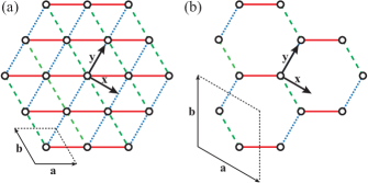
Figure 1: (a) Triangular and (b) honeycomb lattices. Spins are referred to Cartesian axes $\mathbf{x}$, $\mathbf{y}$, and $\mathbf{z}$, with $\mathbf{z}$ directed out of the page. Conventional unit-cell vectors are $\mathbf{a}$, $\mathbf{b}$, and $\mathbf{c}\parallel\mathbf{z}$. The three bond types are shown as solid red, dashed green, and dotted blue lines.

The most general nearest-neighbor spin Hamiltonian allowed by threefold symmetry of the magnetic site has the same form for triangular and honeycomb lattices Rau_2018 ,

$$\mathcal{H} =\sum_{\left\langle i,j\right\rangle}\Bigl{\{}J_{X}\left(S_{i}^{x}S_{j}^{x}+S_{i}^{y}S_{j}^{y}\right)+J_{Z}S_{i}^{z}S_{j}^{z}$$

$$+J_{A}\left[(S_{i}^{x}S_{j}^{x}-S_{i}^{y}S_{j}^{y})\cos\phi_{ij}-(S_{i}^{x}S_{j}^{y}+S_{i}^{y}S_{j}^{x})\sin\phi_{ij}\right]$$

$$-J_{B}\sqrt{2}\left[(S_{i}^{x}S_{j}^{z}+S_{i}^{z}S_{j}^{x})\cos\phi_{ij}+(S_{i}^{y}S_{j}^{z}+S_{i}^{z}S_{j}^{y})\sin\phi_{ij}\right]\Bigr{\}},$$ (1)

where superscript $x$, $y$, and $z$ denote spin components with respect to the $\mathbf{x}$, $\mathbf{y}$, and $\mathbf{z}$ axes shown in Fig. 1, and $\phi_{ij}\in\left\{\frac{2\pi}{3},-\frac{2\pi}{3},0\right\}$ for bonds colored red, green, and blue respectively in Fig. 1. The Hamiltonian contains four interactions, whose physical origin is typically superexchange between trigonally-distorted edge-sharing $M$O₆ octahedra (Rau_2014, ): $J_{X}$ and $J_{Z}$ describe a conventional $XXZ$ model, while $J_{A}$ and $J_{B}$ are bond dependent. Several parameterizations of Eq. (1) are in use (supp, ); I follow the conventions of Ref. Chaloupka_2015, , which resemble those applied to YbMgGaO₄ (Li_2015, ; Shen_2016, ; Paddison_2017, ; Li_2017a, ). A different parameterization $\{J,K,\Gamma,\Gamma^{\prime}\}$ is typically used for honeycomb systems (Rau_2014, ; Chaloupka_2015, ). However, we will see that Eq. (Scattering Signatures of Bond-Dependent Magnetic Interactions) has advantages for interpreting $I(\mathbf{Q})$ data.

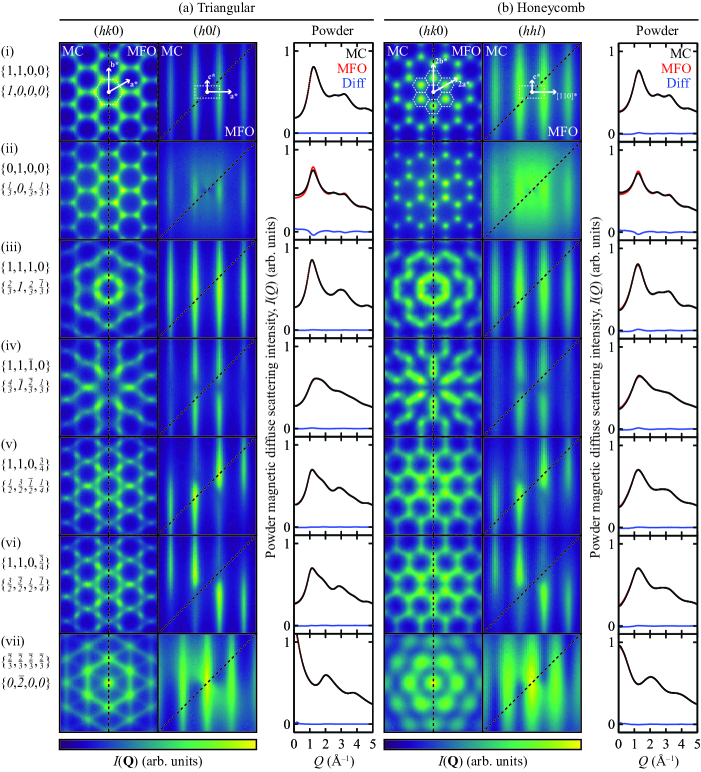
Figure 2: Simulated neutron-diffraction patterns in the paramagnetic phase for test cases (i)–(vii) discussed in the text. The interaction parameters for each model are shown left, with $\{J_{X},J_{Z},J_{A},J_{B}\}$ in roman type above the corresponding $\{J,K,\Gamma,\Gamma^{\prime}\}$ in italics. Column (a) shows calculations for the triangular lattice (left to right: $(hk0)$, $(h0l)$, and powder diffraction patterns) and column (b) shows calculations for the honeycomb lattice (left to right: $(hk0)$, $(hhl)$, and powder diffraction patterns). An isotropic $g$-factor is assumed. Results for Monte Carlo (MC) and reaction-field (MFO) approximations are shown separated by dashed black lines, as labeled on the top panels. For powder patterns, MC results are shown as black circles; MFO results as red lines; and difference (MC–MFO) as blue lines. All powder patterns are shown on the same intensity scale. For single-crystal patterns, reciprocal-lattice vectors $\mathbf{a}^{*}$, $\mathbf{b}^{*}$, and $\mathbf{c}^{*}$ are labeled in the top panels, and the first Brillouin zone is shown as a white dashed line. Both single-crystal planes are shown on the same intensity scale for each test case except honeycomb (i) and (ii), for which the intensity scale is doubled in the $(hhl)$ plane for clarity. In all calculations, the triangular unit cell has dimensions $|\mathbf{a}|=|\mathbf{b}|=3.464\,\text{\AA}$, $|\mathbf{c}|=6.0\,\text{\AA}$, and the honeycomb unit cell has dimensions $|\mathbf{a}|=|\mathbf{b}|=|\mathbf{c}|=6.0\,\text{\AA}$.

I consider seven test cases with interaction parameters $\{J_{X},J_{Z},J_{A},J_{B}\}$ (“$J$’s”) covering a range of interaction space: (i) the antiferromagnetic (AF) Heisenberg model, $\{1,1,0,0\}$; (ii) the AF Ising model, $\{0,1,0,0\}$; (iii, iv) the AF Heisenberg model with $J_{A}=+1$ and $-1$ ($\equiv\bar{1})$, respectively; (v, vi) the AF Heisenberg model with $J_{B}=+\frac{3}{4}$ and $-\frac{3}{4}$, respectively; and (vii) the ferromagnetic Kitaev model, $\{\bar{\frac{2}{3}},\bar{\frac{2}{3}},\bar{\frac{2}{3}},\bar{\frac{2}{3}}\}$, which corresponds to $\{J,K,\Gamma,\Gamma^{\prime}\}=\{0,\bar{2},0,0\}$. Test cases (i) and (ii) are not bond dependent and are included for comparison; (iii)–(vi) explore the effect of changing signs of bond-dependent terms and are potentially relevant to YbMgGaO₄ (Li_2015, ; Shen_2016, ; Paddison_2017, ; Li_2017a, ); and (vii) explores the Kitaev limit potentially relevant to $\alpha$-RuCl₃ (Banerjee_2016, ; Do_2017, ; Banerjee_2017, ; Winter_2017a, ). A further 20 test cases, corresponding to models proposed for $\alpha$-RuCl₃ Laurell_2020 , are considered in SM supp . For test cases (i)–(vii), I performed classical Monte Carlo (MC) simulations of Eq. (Scattering Signatures of Bond-Dependent Magnetic Interactions) with spin length $|\mathbf{S}|=1$ (supp, ). The simulation temperature $T=2$ (in the same units as the $J$’s) for (iii)–(vii) on the triangular lattice, and $T=1$ otherwise, which is well above $T_{N}$ in all cases. The energy-integrated magnetic neutron-diffraction intensity

$$I(\mathbf{Q}) \propto[f(Q)]^{2}\sum_{i,j,\alpha,\beta}p_{\alpha\beta}\bigl{\langle}S_{i}^{\alpha}S_{j}^{\beta}\bigr{\rangle}e^{i\mathbf{Q}\cdot\mathbf{r}_{ij}},$$ (2)

where $\alpha,\beta\in\left\{x,y,z\right\}$ denote Cartesian components, $\mathbf{r}_{ij}$ is the vector connecting spins $i$ and $j$, $f(Q)$ denotes an arbitrary magnetic form factor (Yb³⁺) (Brown_2004, ), and

$$p_{\alpha\beta}\equiv\delta_{\alpha\beta}-Q_{\alpha}Q_{\beta}/Q^{2}$$ (3)

is the projection factor (Lovesey_1987, ; Halpern_1939, ; Paddison_2019, ), which arises because neutrons only “see” spin components perpendicular to $\mathbf{Q}$, and couples spin and spatial degrees of freedom. Eq. (3) is key to magnetic crystallography because it usually allows the absolute spin structure to be solved from $T<T_{N}$ neutron-diffraction data (Shirane_1959, ). I will show that it also allows bond-dependent interactions to be inferred from $T>T_{N}$ neutron-diffraction data.

Fig. 2 shows the single-crystal $I(\mathbf{Q})$ and powder $I(Q)$ Blech_1964 for all test cases. Two orthogonal single-crystal planes are shown: $(hk0)$, and either $(h0l)$ for the triangular lattice or $(hhl)$ for the honeycomb lattice. Our first key result is that $I(\text{{Q})}$ is qualitatively different in each case. In particular, it is strongly affected by changing the sign of $J_{A}$ or $J_{B}$, whereas other experiments (e.g., magnon spectra (Banerjee_2016, ; Ran_2017, ; Ozel_2019, ; Zhang_2018, )) are usually insensitive to at least one of these signs. The differences in the plane perpendicular to $(hk0)$ do not arise from inter-layer interactions—absent in all test cases—but instead from the projection factor, as I now discuss for each test case. (i) The Heisenberg diffraction pattern repeats periodically, except for the trivial decrease of intensity with $f(Q)$. This is because all diagonal correlators $\langle S_{i}^{\alpha}S_{j}^{\alpha}\rangle$ are equal and all off-diagonal correlators $\langle S_{i}^{\alpha}S_{j}^{\beta}\rangle$ are zero; hence $\langle p_{\alpha\alpha}\rangle=2/3$ is independent of $\mathbf{Q}$. (ii) The Ising diffraction pattern repeats periodically in the $(hk0)$ plane but shows further $\mathbf{Q}$-dependence in the perpendicular plane, because the intensity is dominated by $p_{zz}\langle S_{i}^{z}S_{j}^{z}\rangle=(1-Q_{z}^{2}/Q^{2})\langle S_{i}^{z}S_{j}^{z}\rangle$ terms. (iii, iv) Nonzero $J_{A}$ causes nontrivial $\mathbf{Q}$-dependence in both planes because it drives nonzero $\langle S_{i}^{x}S_{j}^{y}\rangle$ and $\langle S_{i}^{y}S_{j}^{x}\rangle$ correlators, so that terms like $p_{xy}\langle S_{i}^{x}S_{j}^{y}\rangle=-Q_{x}Q_{y}\langle S_{i}^{x}S_{j}^{y}\rangle/Q^{2}$ contribute to $I(\mathbf{Q})$. (v, vi) Nonzero $J_{B}$ also causes nontrivial $\mathbf{Q}$-dependence in both planes, but unlike the previous cases, $I(hkl)\neq I(hk\bar{l})$. This is because nonzero $J_{B}$ lowers the hexagonal symmetry of the previous models to trigonal (Chaloupka_2015, ), yielding nonzero terms like $p_{xz}\langle S_{i}^{x}S_{j}^{z}\rangle$ and $p_{yz}\langle S_{i}^{y}S_{j}^{z}\rangle$ that change sign under either $(hkl)\rightarrow(hk\bar{l})$ or $S_{i}^{z}\rightarrow-S_{i}^{z}$ for all $S^{z}$. Since the latter is equivalent to $J_{B}\rightarrow-J_{B}$ in Eq. (Scattering Signatures of Bond-Dependent Magnetic Interactions), both $(hkl)\rightarrow(hk\bar{l})$ and $J_{B}\rightarrow-J_{B}$ have the same effect on $I(\mathbf{Q})$. These results follow from basic properties of Eqs. (Scattering Signatures of Bond-Dependent Magnetic Interactions)–(3) that apply for quantum as well as classical systems, and show that each interaction has a different effect on $I(\mathbf{Q})$. Dominant interactions can therefore be identified by inspection of diffuse-scattering data.

I now obtain a theory that explains the modulation of $I(\mathbf{Q})$. I employ the Onsager reaction-field (MFO) method (Brout_1967, ; Wysin_2000, ) previously shown to give accurate results for Heisenberg models (Logan_1995, ; Eastwood_1995, ; Hohlwein_2003, ; Conlon_2010, ; Bai_2019, ; Plumb_2019, ). The Fourier transform of the interactions $J_{ij}^{\alpha\beta}(\mathbf{Q})\equiv-\sum_{\mathbf{R}}J_{ij}^{\alpha\beta}(\mathbf{R})e^{-\mathrm{i}\mathbf{Q}\cdot\mathbf{R}}$, where $J_{ij}^{\alpha\beta}(\mathbf{R})$ is the coefficient of $S_{i}^{\alpha}S_{j}^{\beta}$ in Eq. (Scattering Signatures of Bond-Dependent Magnetic Interactions) for sites $i$ and $j$ separated by a lattice vector $\mathbf{R}$. The $J_{ij}^{\alpha\beta}(\mathbf{Q})$ are elements of a $3N\times 3N$ interaction matrix, where $N$ is the number of sites in the unit cell. For the triangular lattice ($N=1$), the interaction matrix

$$\mathsf{J}(\mathbf{Q})=-\left(\begin{array}[]{ccc}aJ_{X}+bJ_{A}&cJ_{A}&-\sqrt{2}bJ_{B}\\ cJ_{A}&aJ_{X}-bJ_{A}&\sqrt{2}cJ_{B}\\ -\sqrt{2}bJ_{B}&\sqrt{2}cJ_{B}&aJ_{Z}\end{array}\right),$$ (4)

where $a=2[\cos 2\pi(h+k)+\cos 2\pi h+\cos 2\pi k]$, $b=2\cos 2\pi(h+k)-\cos 2\pi h-\cos 2\pi k$, and $c=\sqrt{3}(\cos 2\pi k-\cos 2\pi h)$. For the honeycomb lattice ($N=2$), the interaction matrix

$$\mathsf{J}_{\mathrm{h}}(\mathbf{Q})=\left(\begin{array}[]{cc}0&\mathsf{J}\\ \mathsf{J}^{*}&0\end{array}\right),$$ (5)

where $a$, $b$, and $c$ in Eq. (4) are replaced by $a_{\mathrm{h}}=1+e^{2\pi\mathrm{i}h}+e^{-2\pi\mathrm{i}k}$, $b_{\mathrm{h}}=e^{-2\pi\mathrm{i}k}-(1+e^{2\pi\mathrm{i}h})/2$, and $c_{\mathrm{h}}=\sqrt{3}(1-e^{2\pi\mathrm{i}h})/2$, respectively. Diagonalizing the interaction matrix at each $\mathbf{Q}$ yields its eigenvalues $\lambda_{\mu}$ and eigenvector components $U_{\mu}^{\alpha,i}$, where $\mu$ labels the $3N$ eigenmodes and $i$ labels sites at positions $\mathbf{r}_{i}$ in the unit cell. The $T>T_{N}$ scattering intensity in the reaction-field approximation is given by

$$I_{\mathrm{MFO}}(\mathbf{Q})\propto\frac{[f(Q)]^{2}}{3N}\sum_{\mu=1}^{3N}\frac{|\mathbf{s}_{\mu}(\mathbf{Q})|^{2}}{1-\chi_{0}(\lambda_{\mu}(\mathbf{Q})-\lambda)},$$ (6)

where $\chi_{0}=1/3T$ is the Curie susceptibility, and $\mathbf{s}_{\mu}(\mathbf{Q})=\sum_{i,\alpha}(\hat{\mathbf{n}}_{\alpha}-\mathbf{Q}\thinspace\hat{\mathbf{n}}_{\alpha}\cdot\mathbf{Q}/Q^{2})U_{\mu}^{\alpha,i}e^{\mathrm{i}\mathbf{Q}\cdot\mathbf{r}_{i}}$ with $\hat{\mathbf{n}}_{\alpha}\in\{\mathbf{x},\mathbf{y},\mathbf{z}\}$. Eq. (6) is identical to the mean-field expression (Enjalran_2004, ) except for the reaction field $\lambda$, which is determined self-consistently by requiring that $\sum_{\mu,\mathbf{q}}[1-\chi_{0}(\lambda_{\mu}(\mathbf{q)}-\lambda)]^{-1}=3NN_{\mathbf{q}}$ for a grid of $N_{\mathbf{q}}=40^{3}$ wavevectors in the Brillouin zone. Fig. 2 compares the single-crystal $I(\mathbf{Q})$ and powder $I(Q)$ from reaction-field theory with the accurate MC results. The agreement is very good in all cases; only in the Ising case are subtle differences evident. The success of reaction-field theory for bond-dependent interactions is remarkable given its simplicity.

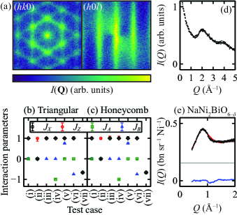
Figure 3: (a) Simulated “noisy” single-crystal data $I(\mathbf{Q})$ with 5% error bars for the Kitaev model on the triangular lattice (test case (vii)). (b,c) Values of the interaction parameters for test cases (i)–(vii) for (b) triangular and (c) honeycomb lattices. In each case, $J_{X}$ is shown as black diamonds, $J_{Z}$ as red circles, $J_{A}$ as green squares, and $J_{B}$ as blue triangles. Error bars indicate values obtained from unconstrained fits of all four parameters to two single-crystal $I(\mathbf{Q})$ planes, such as those shown in (a). (d) Simulated “noisy” powder $I(Q)$ data with 1% error bars for test case (vii). (e) Experimental $I(Q)$ data for NaNi₂BiO_6-δ (black circles), fit (red line), data–fit (blue line), and fitted incoherent level (grey line).

The sensitivity of $I(\mathbf{Q})$ to bond-dependent interactions suggests that it may be possible to solve the inverse problem—to infer interaction values from $I(\mathbf{Q})$ data. To test this possibility, I performed unconstrained fits of the four $J$’s, using MC single-crystal scattering planes as simulated “data” for each test case. To make the tests more realistic, data were adulterated with with random noise drawn from a normal distribution with $\sigma$ equal to 5% of the maximum intensity (“5% error bars”), as shown in Fig. 3(a). An intensity scale factor was also fitted, as required if data are not normalized in absolute intensity units. In the fits, $I(\mathbf{Q})$ was calculated in the reaction-field approximation because it is computationally efficient and free from statistical noise. The nonlinear least-squares algorithm in the Minuit program (James_1975, ) was used to minimize the sum of squared residuals $\chi^{2}$. If the $J$’s are fully determined by the data, a fit should converge to a global minimum $\chi_{\mathrm{min}}^{2}$ with nearly correct $J$’s, provided the initial $J$’s are sufficiently close to optimal. Conversely, if the $J$’s are underdetermined, fits will either fail, or yield several different solutions with indistinguishable fit quality depending on initial $J$’s. A unique solution is defined here as the absence of low-lying false minima with $\chi^{2}<\chi_{\mathrm{min}}^{2}+15$, where this condition reflects the 99% confidence interval for five parameters (James_1994, ). To test for uniqueness, I performed 50 separate fits initialized with different $J$’s randomly distributed in the range $\{-0.5:0.5\}$ Senn_2016 . In every test case, the fits identified a unique solution with nearly correct $J$’s, and convergence was achieved from nearly all (96%) of the initial parameter sets. Similarly favorable results were obtained for 20 $\alpha$-RuCl₃ test cases supp , demonstrating that the approach is robust to inclusion of a third-neighbor interaction and the rapid decay of the Ru³⁺ magnetic form factor Do_2017 . Fig. 3(b,c) shows the systematic error in the optimal $J$’s due to the inaccuracy of the reaction-field approximation. This error is usually small and the worst-case error is $0.14$ in $J_{Z}$. These results show that bond-dependent interactions can be reliably extracted from noisy and unnormalized $I(\mathbf{Q})$ data.

As a more challenging test, I considered powder-averaged $I(Q)$ data with 1% error bars [Fig. 3(d)]. On the one hand, powder averaging causes much information loss. In particular, powder data cannot distinguish $\pm J_{B}$, because $J_{B}\rightarrow-J_{B}$ is equivalent to $(hkl)\rightarrow(hk\bar{l})$; I therefore consider test cases (v, vi) together. On the other hand, $I(Q)$ differs for the other test cases [Fig. 2]. Remarkably, fits of the four $J$’s to noisy $I(Q)$ data yielded a unique optimal solution with nearly correct $J$’s in 10 out of 12 test cases. In the remaining cases—(iii) and (v, vi) for the triangular lattice—two different solutions were identified, which had nearly the same $\chi^{2}$. Parameter uncertainties were also increased compared to single-crystal fits (supp, ). Despite these limitations, the ability of powder fits to identify a small number of candidate models suggests that $I(Q)$ can provide a “fingerprint” of bond-dependent interactions—a compact data set that contains most of the discriminating information.

I finally apply this methodology to published neutron data of the candidate Kitaev material NaNi₂BiO_6-δ ($\delta=0.33$) Scheie_2019 , in which Ni³⁺ ions ($S=3/2$, $J=1/2$) occupy a honeycomb lattice. The experimental $I(Q)$ data shown in Fig. 3(e) were obtained by energy-integrating the $T=10$ K ($>T_{\mathrm{N}}$) inelastic neutron-scattering data of Ref. Scheie_2019, . In the fits, the measured magnetic moment of $2.21(1)$ $\mu_{\mathrm{B}}$ per Ni³⁺ was assumed Scheie_2019 , and an incoherent (flat-in-$Q$) signal was fitted. For all fits, the magnitude of $K$ is at least twice that of $J$, $\Gamma$, and $\Gamma^{\prime}$, and the predicted in-plane magnetic ordering wavevector $\mathbf{k}\approx({\frac{1}{3},\frac{1}{3}})$ is consistent with the measured value Scheie_2019 . These results demonstrate the successful application of our methodology to experimental data and support the dominant Kitaev interactions proposed in NaNi₂BiO_6-δ Scheie_2019 .

These results show that bond-dependent interactions on triangular and honeycomb lattices have signatures in diffuse neutron-scattering data at $T>T_{N}$ that enable estimation of the interactions via unconstrained fits. This unexpected sensitivity is mainly due to the projection factor, Eq. (3); hence, it is important to measure $I(\mathbf{Q})$ outside the $(hk0)$ plane where this factor is significant, and to include it in calculations, which has not often been done. Our methodology is generally applicable and employs conventional least-squares optimization (Bai_2019, ), providing a robust and computationally-efficient alternative to machine-learning-based approaches (Samarakoon_2020, ), as well as to interaction-independent approaches such as reverse Monte Carlo refinement (Paddison_2012, ) and pair-distribution-function analysis (Frandsen_2014, ). Key advantages are that measurements in high magnetic fields are not required, and additional data such as bulk magnetic susceptibility—related to $I(Q\rightarrow 0)$ Marshall_1968 —can be included. A limitation is that quantum effects that redistribute scattering intensity (Mourigal_2013, ; Samarakoon_2017, ) are not included: this may cause inaccuracy in fitted interaction values, but does not affect sensitivity to interaction signs. Moreover, a fit typically requires only a few hundred $I(\mathbf{Q})$ calculations for convergence—taking $\sim$$60$ s to fit to $\sim$$10^{4}$ data points on a laptop—so that replacement of classical calculations by more-expensive quantum calculations is feasible. If interlayer spin correlations are negligible above $T_{N}$, our results are unaffected by the layer stacking sequence—a useful feature because of the prevalence of stacking faults in quasi-2D materials (Johnson_2015, ). These results promise to accelerate experimental determination of spin Hamiltonians of candidate materials that do not exhibit conventional magnetic ordering, such as in the emerging field of “topology by design” metal-organic frameworks (Yamada_2017, ).

I am grateful to Xiaojian Bai (ORNL), Andrew Christianson (ORNL), Seung-Hwan Do (ORNL), Mechthild Enderle (ILL), Andrew Goodwin (Oxford), Pontus Laurell (ORNL), Martin Mourigal (Georgia Tech), Kate Ross (Colorado State), Allen Scheie (ORNL), Ross Stewart (ISIS), and Alan Tennant (ORNL) for valuable discussions. I also thank the authors of Ref. Scheie_2019, for making available their published data. This work was supported by the Laboratory Directed Research and Development Program of Oak Ridge National Laboratory, managed by UT-Battelle, LLC for the US Department of Energy (project design, calculations, and manuscript writing), and by the U.S. Department of Energy, Office of Science, Basic Energy Sciences, Materials Sciences and Engineering Division (computational resources). I acknowledge a Junior Research Fellowship from Churchill College, University of Cambridge, during which computer programs underlying this work were written.

References

- (1) A. Kitaev, Ann. Phys. 303, 2 (2003).
- (2) C. Nayak, S. H. Simon, A. Stern, M. Freedman, S. Das Sarma, Rev. Mod. Phys. 80, 1083 (2008).
- (3) H. Takagi, T. Takayama, G. Jackeli, G. Khaliullin, S. E. Nagler, Nat. Rev. Phys. 1, 264 (2019).
- (4) C. Broholm, R. J. Cava, S. A. Kivelson, D. G. Nocera, M. R. Norman, T. Senthil, Science 367 (2020).
- (5) G. Baskaran, S. Mandal, R. Shankar, Phys. Rev. Lett. 98, 247201 (2007).
- (6) M. Hermanns, I. Kimchi, J. Knolle, Ann. Rev. Condens. Matt. Phys. 9, 17 (2018).
- (7) I. Rousochatzakis, Y. Sizyuk, N. B. Perkins, Nature Communications 9, 1575 (2018).
- (8) G. Jackeli, G. Khaliullin, Phys. Rev. Lett. 102, 017205 (2009).
- (9) J. Chaloupka, G. Jackeli, G. Khaliullin, Phys. Rev. Lett. 105, 027204 (2010).
- (10) S. M. Winter, A. A. Tsirlin, M. Daghofer, J. van den Brink, Y. Singh, P. Gegenwart, R. Valentí, J. Phys.: Condens. Matter 29, 493002 (2017).
- (11) R. Sano, Y. Kato, Y. Motome, Phys. Rev. B 97, 014408 (2018).
- (12) K. W. Plumb, J. P. Clancy, L. J. Sandilands, V. V. Shankar, Y. F. Hu, K. S. Burch, H.-Y. Kee, Y.-J. Kim, Phys. Rev. B 90, 041112 (2014).
- (13) A. Banerjee, C. A. Bridges, J. Q. Yan, A. A. Aczel, L. Li, M. B. Stone, G. E. Granroth, M. D. Lumsden, Y. Yiu, J. Knolle, S. Bhattacharjee, D. L. Kovrizhin, R. Moessner, D. A. Tennant, D. G. Mandrus, S. E. Nagler, Nat. Mater. 15, 733 (2016).
- (14) S.-H. Do, S.-Y. Park, J. Yoshitake, J. Nasu, Y. Motome, Y. S. Kwon, D. T. Adroja, D. J. Voneshen, K. Kim, T. H. Jang, J. H. Park, K.-Y. Choi, S. Ji, Nat. Phys. 13, 1079 (2017).
- (15) A. Banerjee, J. Yan, J. Knolle, C. A. Bridges, M. B. Stone, M. D. Lumsden, D. G. Mandrus, D. A. Tennant, R. Moessner, S. E. Nagler, Science 356, 1055 (2017).
- (16) S. M. Winter, K. Riedl, P. A. Maksimov, A. L. Chernyshev, A. Honecker, R. Valentí, Nat. Commun. 8, 1152 (2017).
- (17) G. Sala, M. B. Stone, B. K. Rai, A. F. May, D. S. Parker, G. B. Halász, Y. Q. Cheng, G. Ehlers, V. O. Garlea, Q. Zhang, M. D. Lumsden, A. D. Christianson, Phys. Rev. B 100, 180406 (2019).
- (18) A. Scheie, K. Ross, P. P. Stavropoulos, E. Seibel, J. A. Rodriguez-Rivera, J. A. Tang, Y. Li, H.-Y. Kee, R. J. Cava, C. Broholm, Phys. Rev. B 100, 214421 (2019).
- (19) K. Kitagawa, T. Takayama, Y. Matsumoto, A. Kato, R. Takano, Y. Kishimoto, S. Bette, R. Dinnebier, G. Jackeli, H. Takagi, Nature 554, 341 (2018).
- (20) R. Yadav, R. Ray, M. S. Eldeeb, S. Nishimoto, L. Hozoi, J. van den Brink, Phys. Rev. Lett. 121, 197203 (2018).
- (21) Y. Singh, S. Manni, J. Reuther, T. Berlijn, R. Thomale, W. Ku, S. Trebst, P. Gegenwart, Phys. Rev. Lett. 108, 127203 (2012).
- (22) J. G. Rau, E. K.-H. Lee, H.-Y. Kee, Phys. Rev. Lett. 112, 077204 (2014).
- (23) S. Hwan Chun, J.-W. Kim, J. Kim, H. Zheng, C. C. Stoumpos, C. D. Malliakas, J. F. Mitchell, K. Mehlawat, Y. Singh, Y. Choi, T. Gog, A. Al-Zein, M. M. Sala, M. Krisch, J. Chaloupka, G. Jackeli, G. Khaliullin, B. J. Kim, Nat. Phys. 11, 462 (2015).
- (24) S. C. Williams, R. D. Johnson, F. Freund, S. Choi, A. Jesche, I. Kimchi, S. Manni, A. Bombardi, P. Manuel, P. Gegenwart, R. Coldea, Phys. Rev. B 93, 195158 (2016).
- (25) S. Choi, S. Manni, J. Singleton, C. V. Topping, T. Lancaster, S. J. Blundell, D. T. Adroja, V. Zapf, P. Gegenwart, R. Coldea, Phys. Rev. B 99, 054426 (2019).
- (26) Z. Zhu, P. A. Maksimov, S. R. White, A. L. Chernyshev, Phys. Rev. Lett. 120, 207203 (2018).
- (27) Y. Li, G. Chen, W. Tong, L. Pi, J. Liu, Z. Yang, X. Wang, Q. Zhang, Phys. Rev. Lett. 115, 167203 (2015).
- (28) Y. Shen, Y.-D. Li, H. Wo, Y. Li, S. Shen, B. Pan, Q. Wang, H. C. Walker, P. Steffens, M. Boehm, Y. Hao, D. L. Quintero-Castro, L. W. Harriger, M. D. Frontzek, L. Hao, S. Meng, Q. Zhang, G. Chen, J. Zhao, Nature 540, 559 (2016).
- (29) J. A. M. Paddison, M. Daum, Z. Dun, G. Ehlers, Y. Liu, M. B. Stone, H. Zhou, M. Mourigal, Nat. Phys. 13, 117 (2017).
- (30) Y. Li, D. Adroja, D. Voneshen, R. I. Bewley, Q. Zhang, A. A. Tsirlin, P. Gegenwart, Nat. Commun. 8, 15814 (2017).
- (31) M. Baenitz, P. Schlender, J. Sichelschmidt, Y. A. Onykiienko, Z. Zangeneh, K. M. Ranjith, R. Sarkar, L. Hozoi, H. C. Walker, J.-C. Orain, H. Yasuoka, J. van den Brink, H. H. Klauss, D. S. Inosov, T. Doert, Phys. Rev. B 98, 220409 (2018).
- (32) R. Sarkar, P. Schlender, V. Grinenko, E. Haeussler, P. J. Baker, T. Doert, H.-H. Klauss, Phys. Rev. B 100, 241116 (2019).
- (33) M. M. Bordelon, E. Kenney, C. Liu, T. Hogan, L. Posthuma, M. Kavand, Y. Lyu, M. Sherwin, N. P. Butch, C. Brown, M. J. Graf, L. Balents, S. D. Wilson, Nat. Phys. 15, 1058 (2019).
- (34) L. Ding, P. Manuel, S. Bachus, F. Grußler, P. Gegenwart, J. Singleton, R. D. Johnson, H. C. Walker, D. T. Adroja, A. D. Hillier, A. A. Tsirlin, Phys. Rev. B 100, 144432 (2019).
- (35) P. Laurell, S. Okamoto, npj Quantum Mater. 5, 2 (2020).
- (36) J. Chaloupka, G. Khaliullin, Phys. Rev. B 92, 024413 (2015).
- (37) K. Ran, J. Wang, W. Wang, Z.-Y. Dong, X. Ren, S. Bao, S. Li, Z. Ma, Y. Gan, Y. Zhang, J. T. Park, G. Deng, S. Danilkin, S.-L. Yu, J.-X. Li, J. Wen, Phys. Rev. Lett. 118, 107203 (2017).
- (38) I. O. Ozel, C. A. Belvin, E. Baldini, I. Kimchi, S. Do, K.-Y. Choi, N. Gedik, Phys. Rev. B 100, 085108 (2019).
- (39) X. Zhang, F. Mahmood, M. Daum, Z. Dun, J. A. M. Paddison, N. J. Laurita, T. Hong, H. Zhou, N. P. Armitage, M. Mourigal, Phys. Rev. X 8, 031001 (2018).
- (40) K. A. Ross, L. Savary, B. D. Gaulin, L. Balents, Phys. Rev. X 1, 021002 (2011).
- (41) P. Lampen-Kelley, A. Banerjee, A. A. Aczel, H. B. Cao, M. B. Stone, C. A. Bridges, J.-Q. Yan, S. E. Nagler, D. Mandrus, Phys. Rev. Lett. 119, 237203 (2017).
- (42) Z. Zhu, P. A. Maksimov, S. R. White, A. L. Chernyshev, Phys. Rev. Lett. 119, 157201 (2017).
- (43) Y. Li, D. Adroja, R. I. Bewley, D. Voneshen, A. A. Tsirlin, P. Gegenwart, Q. Zhang, Phys. Rev. Lett. 118, 107202 (2017).
- (44) R. Sarkar, Z. Mei, A. Ruiz, G. Lopez, H.-H. Klauss, J. G. Analytis, I. Kimchi, N. J. Curro, Phys. Rev. B 101, 081101 (2020).
- (45) S. M. Winter, Y. Li, H. O. Jeschke, R. Valentí, Phys. Rev. B 93, 214431 (2016).
- (46) I. A. Blech, B. L. Averbach, Physics 1, 31 (1964).
- (47) P. Manuel, L. C. Chapon, P. G. Radaelli, H. Zheng, J. F. Mitchell, Phys. Rev. Lett. 103, 037202 (2009).
- (48) T. Fennell, P. P. Deen, A. R. Wildes, K. Schmalzl, D. Prabhakaran, A. T. Boothroyd, R. J. Aldus, D. F. McMorrow, S. T. Bramwell, Science 326, 415 (2009).
- (49) X. Bai, J. A. M. Paddison, E. Kapit, S. M. Koohpayeh, J.-J. Wen, S. E. Dutton, A. T. Savici, A. I. Kolesnikov, G. E. Granroth, C. L. Broholm, J. T. Chalker, M. Mourigal, Phys. Rev. Lett. 122, 097201 (2019).
- (50) A. M. Samarakoon, K. Barros, Y. W. Li, M. Eisenbach, Q. Zhang, F. Ye, V. Sharma, Z. L. Dun, H. Zhou, S. A. Grigera, C. D. Batista, D. A. Tennant, Nat. Commun. 11, 892 (2020).
- (51) J. G. Rau, M. J. P. Gingras, Phys. Rev. B 98, 054408 (2018).
- (52) See supplementary information at [URL will be inserted by publisher] for relations between Hamiltonian parameterizations, details of Monte Carlo simulations, additional test cases for -RuCl3, and fit statistics.
- (53) P. J. Brown, International Tables for Crystallography (Kluwer Academic Publishers, Dordrecht, 2004), vol. C, chap. Magnetic Form Factors, pp. 454–460.
- (54) S. W. Lovesey, Theory of Neutron Scattering from Condensed Matter: Polarization Effects and Magnetic Scattering, vol. 2 (Oxford University Press, Oxford, 1987).
- (55) O. Halpern, M. H. Johnson, Phys. Rev. 55, 898 (1939).
- (56) J. A. M. Paddison, Acta Crystallogr. A 75, 14 (2019).
- (57) G. Shirane, Acta Crystallogr. 12, 282 (1959).
- (58) R. Brout, H. Thomas, Physics Physique Fizika 3, 317 (1967).
- (59) G. M. Wysin, Phys. Rev. B 62, 3251 (2000).
- (60) D. E. Logan, Y. H. Szczech, M. A. Tusch, Europhys. Lett. (EPL) 30, 307 (1995).
- (61) M. P. Eastwood, D. E. Logan, Phys. Rev. B 52, 9455 (1995).
- (62) D. Hohlwein, J.-U. Hoffmann, R. Schneider, Phys. Rev. B 68, 140408 (2003).
- (63) P. H. Conlon, J. T. Chalker, Phys. Rev. B 81, 224413 (2010).
- (64) K. W. Plumb, H. J. Changlani, A. Scheie, S. Zhang, J. W. Krizan, J. A. Rodriguez-Rivera, Y. Qiu, B. Winn, R. J. Cava, C. L. Broholm, Nat. Phys. 15, 54 (2019).
- (65) M. Enjalran, M. J. P. Gingras, Phys. Rev. B 70, 174426 (2004).
- (66) F. James, M. Roos, Comp. Phys. Commun. 10, 343 (1975).
- (67) F. James, MINUIT Function Minimization and Error Analysis: Reference Manual Version 94.1, CERN (1994).
- (68) M. S. Senn, D. A. Keen, T. C. A. Lucas, J. A. Hriljac, A. L. Goodwin, Phys. Rev. Lett. 116, 207602 (2016).
- (69) J. A. M. Paddison, A. L. Goodwin, Phys. Rev. Lett. 108, 017204 (2012).
- (70) B. A. Frandsen, X. Yang, S. J. L. Billinge, Acta Crystallogr. A 70, 3 (2014).
- (71) W. Marshall, R. D. Lowde, Rep. Prog. Phys. 31, 705 (1968).
- (72) M. Mourigal, W. T. Fuhrman, A. L. Chernyshev, M. E. Zhitomirsky, Phys. Rev. B 88, 094407 (2013).
- (73) A. M. Samarakoon, A. Banerjee, S.-S. Zhang, Y. Kamiya, S. E. Nagler, D. A. Tennant, S.-H. Lee, C. D. Batista, Phys. Rev. B 96, 134408 (2017).
- (74) R. D. Johnson, S. C. Williams, A. A. Haghighirad, J. Singleton, V. Zapf, P. Manuel, I. I. Mazin, Y. Li, H. O. Jeschke, R. Valentí, R. Coldea, Phys. Rev. B 92, 235119 (2015).
- (75) M. G. Yamada, H. Fujita, M. Oshikawa, Phys. Rev. Lett. 119, 057202 (2017).