Extending the RISC-V ISA for Efficient RNN-based 5G Radio Resource Management

Abstract

Radio Resource Management (RRM) in 5G mobile communication is a challenging problem for which Recurrent Neural Networks (RNN) have shown promising results. Accelerating the compute-intensive RNN inference is therefore of utmost importance. Programmable solutions are desirable for effective 5G-RRM top cope with the rapidly evolving landscape of RNN variations. In this paper, we investigate RNN inference acceleration by tuning both the instruction set and micro-architecture of a micro-controller-class open-source RISC-V core. We couple HW extensions with software optimizations to achieve an overall improvement in throughput and energy efficiency of 15$\times$ and 10$\times$ w.r.t. the baseline core on a wide range of RNNs used in various RRM tasks.

I Introduction

Radio Resource Management is challenging as it aims at achieving maximum utilization of the limited publicly available frequency bands [1], under highly heterogeneous traffic (e.g., tiny sensor-nodes vs. mobile routers), and rapidly varying radio signal propagation conditions. Notably, RRM tasks have to be executed in the frame of milliseconds, which exclude compute-intensive algorithms [2]. Presently, 5G applications impose strict new intensive requirements on radio communication systems: 1) very high reliability and low-latency for autonomous vehicles, 2) very high bandwidth requirements for video telephony and virtual reality, and 3) massive machine-to-machine communication for the Internet of Things. These challenging requirements ask for extending the existing cellular network with more antennas, improving antenna efficiency, and more effective RRM. Therefore, more advanced allocation algorithms are required to distribute limited resources (e.g., frequency bands, transmit power, data rates) to mobile clients efficiently.

Typically, RRM problems have been modeled with full observability and solving convex problems with traditional optimization approaches. Exhaustive search methods led to very high computation costs [3], and sub-optimal solutions based on Lagrangian relaxation, iterative distribution optimization, and other heuristic approaches had convergence issues and lacked guarantees [3]. Traditional methods like the weighted sum-rate MSE algorithm [4] and fractional programming [5] are iterative, and most of them need to perform complex operations (e.g., matrix inversion or SVD) in every single iteration. It is, therefore, extremely challenging to push these methods to the throughput and scale required for 5G-RRM. Recently, neural networks have gained increasing attention for 5G-RRM. At the physical layer, RNNs have been used to compensate for imperfections and nonlinearities and collision detection in the RF domain [6, 7]. This is getting even more important for high-frequency communication, where absorption starts to strongly depend on the environment, and for ultra-dense cell networks where cross-tier interference has to be compensated [8]. Classic multi-layer perceptron [9, 10, 11, 12], (recurrent) Long Short-Term Memories LSTM [13, 14], and Convolution Neural Networks [15] have been used at the data-link layer, which is responsible for resource allocation, including dynamic resource scheduling of frequency bands, dynamic range, and handover control. Reinforcement learning-based deep Q-Learning networks [16] have been used for several typical RRM problems like dynamic spectrum access utilization [14, 9, 17], power level selection [9, 10, 12], rate control [10], and time-slotted optimization [11].

These networks are less computationally demanding than classical RRM algorithms, but they are far from trivial. Specialized and efficient stand-alone Neural Networks accelerators have been presented recently [18]. Nevertheless, hardwired RNN accelerators cannot cope with the flexibility requirements found in a typical RRM setting, as base stations typically stay in the field for a very long time, while RRM algorithms are rapidly evolving. FPGA-based acceleration has been explored for RNN inference to retain flexibility. For instance, LSTM acceleration on FPGA achieving up to 13 GMAC/s/W, has been presented in Cao et al. [19] and Gao et al.[20]. To further increase efficiency, compression techniques (e.g., block-circulant weight matrices, pruning with zero-skipping [20, 19]) have been applied, and a top (effective) energy efficiency of 82 GMAC/s/W on a Xilinx Zynq-7100 FPGA has been presented [20]. Nevertheless, these compression schemes have not yet been proven to work for the networks used in the RRM field, and FPGAs have a cost envelope that is not compatible with massive and dense deployment, as required in 5G networks. To address this intertwined flexibility, efficiency, and cost challenges, we propose to enhance the open and royalty-free RISC-V ISA and leverage the availability of high-quality open-source cores based on this widely supported ISA. We demonstrate a micro-controller class RISC-V core with RNN-enhancements for RRM acceleration, and we couple hardware extensions with software optimizations. We achieve an energy efficiency of 218 GMAC/s/W, and a throughput of 566 MMAC/s, which is an improvement of 10$\times$ and 15$\times$, respectively, over the baseline open-source core. Such an order-of-magnitude boost is obtained thanks to data reuse with output feature map tiling (1.9$\times$), adding custom activation instructions (13% within LSTMs), merging load and compute (1.15$\times$/1.7$\times$), and input FM tiling (5%).

The proposed extensions maintain backward compatibility with the baseline RISC-V ISA and have a very small overhead (3.4%) in area and no increase in the longest path. Improvements are consistently achieved over a quite diverse set of RNNs used for various RRM tasks, thereby confirming the flexibility of our approach.

II Related Works

II-A ML Compute Platforms

With the machine learning revolution, a variety of different ML compute platforms have been presented in industry and academia, spanning from high-performance server accelerators (e.g., Google’s TPU cores) to embedded platforms (e.g., Nvidia Jetson Xavier) to stand-alone application-specific accelerators [18]. We are not aware of any RNN acceleration engine targeting RRM applications. General-purpose processors have been extended with new matrix and vector extensions to handle the common compute patterns in Neural Networks. In the Advanced Vector Extensions AVC-512 of the x86 ISA, Intel added the VNNIW instruction extension, which include 16$\times$32-bit SIMD vector operation for efficient convolution kernels in single-precision float FP16 and accumulations in double-precision float FP32 and since Cascade Lake (2019) the fixed-point version (VNNI) with 8-bit (e.g., VPDBUSD) and 16-bit (e.g., VPDBUSSD) vector product with 32-bit accumulation [21]. The AARCH64 Neon extensions in the ARMv8-A processor series provides special SIMD instructions for sum-dot-products (e.g., BFDOT) and 2$\times$2 matrix-matrix multiplications (e.g., BFMMLA) with 2-way SIMD in brain floating-point format bfloat16. Recently, ARM presented the M-profile Vector Extensions MVE (Helium) for their embedded processor family Cortex-M. Helium instructions feature computations in various SIMD-formats (INT8/16/32, FP16/32), hardware loops, interleaved post-increment load/stores [22]. However, Intel typically focuses on the high-performance high-cost processor market, and the Helium extensions are not yet available in HW implementations.

Besides ISA extension, also highly-optimized SW kernels have been developed exploiting these instructions. These include utilizing parallel SIMD computations (e.g., 16-bit [23], 8-bit [24]) and data reuse with appropriate tiling. Tiling helps to reduce data loads from memory and reuse data with the local registerfile. Output FM tiling (OFM), where several outputs are calculated in parallel and input FM loads can be shared, has been commonly used (e.g., [23, 24]). Furthermore, convolutional layers can be reformulated as matrix-matrix multiplications with the im2col technique [25]. This allows to tile both the input and output FM spatially in $m\times n$-sized tiles and thus reduces the number of loads from $\mathcal{O}(mn)$ to $\mathcal{O}(m+n)$, as both weights and input FM pixels can be reused. Previous work has mainly focused on on CNNs [23, 24]. Still, this two-dimensional tiling cannot be applied to (non-convolutional) LSTMs and Linear Layers, which are the main network kernels used in RRM applications.

Neural Networks are commonly trained in floating-point format. Still, recently, it has been shown that integer-aware training allows us to use more energy and area efficient fixed-point without any significant accuracy drop, especially 16-bit quantization [26], but even eight and fewer bits [27].

Finally, RNNs use transcendental activation functions, which are computationally complex. Previously, there have been 4 approaches to accelerate the computation of these functions: piecewise linear approximation (PLA)[23], low-order Taylor series expansion (e.g., 2nd order [28]), LUT with adaptive value granularity [29], or a small neural network [30]. We use a PLA approach, but differently from previous work, we exploit the symmetry property of tanh and sig, we take into account fixed-point quantization and evaluate in detail the error introduced by different numbers of interpolation intervals, rather than selecting a high number of intervals (i.e., 128 in ARM’s CMSIS-NN [23]).

II-B RISC-V and RI5CY

The RISC-V ISA [31] has recently become the de facto standard in open-source and free instruction set architecture. RISC-V provides plenty of encoding space for extensions and is therefore suitable for application-driven processor customization while maintaining compatibility with the baseline ISA. In this work, we rely on the RI5CY [32], a high-quality, silicon-proven, and open-source core supporting the standard RISC-V RV32IMFC ISA (including integer, integer multiplications, single-precision floating-point, and compressed instructions). Additionally, RI5CY supports the Xpulp ISA extensions featuring extended fixed-point support (e.g., on-the-fly re-quantization and saturation), SIMD instructions, post-increment store and loads, and hardware loops.

II-C Benchmark Suite and Neural Networks

We have selected an application benchmark consisting of 10 neural networks which have been presented recently in the RRM domain. These networks differ in network types (Fully-Connected Neural Layers ([9, 2, 11, 33, 12, 3, 17], Long-short Term Memories [13, 14], Convolutional Neural Network [15]), learning methods (Supervised [13, 2, 33, 15], reinforcement-based [14, 9, 11, 12, 17], unsupervised [3]), application (cellular networks [13, 3], peer-to-peer communication [14], wireless communication systems [11, 33, 12, 15, 17], wired communication [2]), and optimization metric (throughput [13, 14, 2, 11, 33, 12, 3, 15, 17], fairness [13, 14], latency [9], energy efficiency [15]). A detailed description of the networks can be found in the project report [34]. Three main ML kernels are used within these networks: Fully-connected layers (or Multi-Layer Perceptron MLP), Long-short Term Memories LSTM, and Convolutional Neural Network CNN Layer. A fully-connected layer connects all input (neurons) $\mathbf{x}\in\mathbb{R}^{m}$ to all outputs (neurons) $\mathbf{o}\in\mathbb{R}^{n}$ and is described with the following matrix-vector multiplication and the corresponding weight matrix $\mathbf{W}\in\mathbb{R}^{n\times m}$: $\mathbf{o}=\mathbf{b}+\mathbf{W}\mathbf{x}$. LSTM are recurrent networks able to learn time series and are described by $m$ input neurons and $n$ internal memory cells $c_{t}$, $n$ hidden states $h_{t}$ and the corresponding matrix-vector multiplications, point-wise vector-vector multiplications/additions (i.e., Hadamard product $\mathbf{a}\circ\mathbf{b}=(a_{i}\cdot b_{i})_{i}$), and point-wise application of sigmoid and hyperbolic tangent activation functions:

$$\mathbf{o_{t}}(x_{t},h_{t-1}) =\text{sig}(\mathbf{W_{o}}\mathbf{x_{t}}+\mathbf{U_{o}}\mathbf{h_{t-1}}+\mathbf{b_{o}})$$ (1)

$$\mathbf{f_{t}}(x_{t},h_{t-1}) =\text{sig}(\mathbf{W_{f}}\mathbf{x_{t}}+\mathbf{U_{f}}\mathbf{h_{t-1}}+\mathbf{b_{f}})$$ (2)

$$\mathbf{i_{t}}(x_{t},h_{t-1}) =\text{sig}(\mathbf{W_{i}}\mathbf{x_{t}}+\mathbf{U_{i}}\mathbf{h_{t-1}}+\mathbf{b_{i}})$$ (3)

$$\mathbf{g_{t}}(x_{t},h_{t-1}) =\text{tanh}(\mathbf{W_{c}}\mathbf{x_{t}}+\mathbf{U_{c}}\mathbf{h_{t-1}}+\mathbf{b_{c}})$$ (4)

$$\mathbf{c_{t}}(x_{t},c_{t-1}) =\mathbf{f_{t}}\circ\mathbf{c_{t-1}}+\mathbf{i_{t}}\circ\mathbf{g_{t}}$$ (5)

$$\mathbf{h_{t}}(o_{t},c_{t}) =\mathbf{o_{t}}\circ\text{tanh}(\mathbf{c_{t})}$$ (6)

Whereas the weight matrices $W_{o},W_{f},W_{i},W_{g}\in\mathbb{R}^{n\times m}$ and $U_{o},$ $U_{f},U_{i},\allowbreak U_{c}\in\mathbb{R}^{m\times m}$ and bias vectors $b_{o},b_{f},b_{i},b_{c}\in\mathbb{R}^{m}$.

Finally, CNN layers exploit the translation invariance in the data (e.g., in images) and map $n$ $h_{im,in}\times w_{im,in}$-sized input channels $i_{n}\in\mathbb{R}^{h_{im,in}\times w_{im,in}}$ $k$ $h_{im,out}\times w_{im,out}$-sized output channel maps by applying $h_{k}\times b_{k}$-sized convolution filters $w_{k,n}\in\mathbb{R}^{h_{k}\times b_{k}}$ to every input channel for every output channel.

$$\mathbf{o_{k}}=\mathbf{C_{k}}+\sum_{n\in I}\underbrace{{\mathbf{i_{n}}\ast\mathbf{w_{k,n}}}}_{\mathbf{\tilde{o}_{k,n}}}$$

$$=C_{k}+\sum_{n\in I}\underbrace{\Bigg{(}\sum^{b_{k}-1}_{a=0}\sum^{h_{k}-1}_{b=0}{i_{n}\left(x+a,y+b\right)\cdot w_{k,n}(a,b)}\Bigg{)}}_{\tilde{o}_{k,n}(x,y)}$$

III HW/SW Extension and Optimizations

TABLE I: Cycle and Instruction Count Optimizations for the entire RRM benchmark suite (RISCY in bold, new ext. in blue)

a) w/o opt (RV32IMC)

b) +SIMD/HWL (Xpulp)

c) +Out-FM Tile./tanh/sig

d) +pl.sdotsp instruction

e) +Input FM Tiling

Instr.

kcycles

kinstrs

Instr.

kcyc.

kinstrs

Instr.

kcyc.

kinstrs

Instr.

kcyc.

kinstrs

Instr.

kcyc.

kinstrs

addi

3’269

3’269

lw!

2’432

1’621

lw!

894

893

pl.sdot

811

811

pl.sdot

817

817

bltu

3’248

1’627

pv.sdot

811

811

pv.sdot

811

811

lw!

166

83

lw!

83

83

lh

3’248

3’248

addi

22

22

lw

9

9

lw

9

9

lw

39

35

sw

1’627

1’627

jal

10

5

sw

8

8

sw

8

8

sw

16

16

lw

1’627

1’627

sh

10

10

add

7

6

add

7

6

d.srai

8

8

mac

1’621

1’621

srai

10

10

tanh,sig

0.4

0.4

tanh,sig

0.4

0.4

tanh,sig

0.4

0.4

oth.

43

32

oth.

28

27

oth.

26

26

oth.

30

29

oth.

17

10

$\Sigma$

14’683

13’051

$\Sigma$

3’323

2’506

$\Sigma$

1’756

1’753

$\Sigma$

1’028

943

$\Sigma$

980

969

Impr.

Baseline (1$\times$)

Impr.

4.4$\times$

Impr.

8.4$\times$ (1.9$\times$)

Impr.

14.3$\times$ (1.7$\times$)

Impr.

15.0$\times$ (1.05$\times$)

III-A Baseline Implementation (SW)

We have developed a straight-forward implementation (e.g., organizing matrix-vector multiplication as a double nested loop over all inputs and outputs) of all required network kernels in C where weights and data values are encoded in 16-bit fixed-point format (i.e, $Q_{3.12}$). This format offers a good compromise between accuracy/robustness and energy-efficiency/throughput, and most importantly, does not require fixed-point aware retraining that would be necessary for smaller bit-widths. The C implementation is compiled with standard GCC 7.1.1 for RISC-V RV32IMFC ISA and was run on the RI5CY core. The instruction count for the entire benchmark suite is shown in Tab. Ia and is used as the baseline for further comparisons.

III-B SIMD, HWL and post-increment load (HW)

As a first optimization step, we re-wrote the code to exploit Xpulp extensions as much as possible. The 16-bit data (weights and inputs) are packed into the packed SIMD vector format (i.e., v2s), allowing the compiler to map every two subsequent input FM $p(2c_{i})$ and $p(2c_{i}+1)$ and the corresponding weights $(c_{o},2c_{i})$ and $w(c_{o},2c_{i}+1)$ to a mac using a single pv.sdotsp.h instruction without the need of custom intrinsics.

$$o(c_{o}) =b(c_{o})+\sum_{c_{i}=0}^{c_{in}/2}\begin{pmatrix}p(2c_{i})\\ p(2c_{i}+1)\end{pmatrix}\begin{pmatrix}w(c_{o},2c_{i})\\ w(c_{o},2c_{i}+1)\end{pmatrix}$$ (7)

The next optimization is to reduce the overhead of loop control instructions in small loop bodies that are seen in such operations by using hardware loops that are part of the Xpulp extensions. The hardware loop does not use any additional instructions during the loop execution, but requires loop index manipulation instructions (i.e., pl.setup) to set three registers: a loop counter (rB), the loop start PC+4 and the loop end (PC+rA). When the PC reaches the loop end, the controller decrements the loop counter and jumps back to the loop start until the loop counter reaches zero.

The final optimization is to take advantage of post-increment load-word instruction (i.e., lw!) to increment the data pointer for weights and input feature maps at the same time as executing the load word instruction, saving a separate addi instruction in the process. Combining these three techniques results in 4.4$\times$ reduction w.r.t. to the unmodified RISC-V IMC baseline in the number of instructions executed as can be seen in Tab. Ib.

III-C Output Feature Map Tiling (SW)

To compute one MAC two loads to the memory are needed: one for the weight and one for the value of the corresponding input neuron. Fortunately, the read for the input value can be reused for several outputs. The output features are therefore organized in tiles of $N$ output channels and the contribution of the input neurons is calculated for all output neurons of the current input neuron. These partial sums can be stored in registers and are not written back to the memory until all input activations have been weighted and accumulated. Algorithm 1 gives an overview of the implementation and scheduling of the output FM tiling.

Algorithm 1 Fully-Connected Layer with Output FM Tiling

0:  All weights $w_{mn}$ and input activations $i_{m}$ for all input channels $m\in c_{in}$ and output channels $n\in c_{out}$ in memory

1:  for all d-sized output channel tiles $\tilde{o}_{k}=\{o_{k\cdot d},...,o_{(k+1)\cdot d}\}$ do

2:     for all output channels $o_{l}$ in $\tilde{o}_{k}$ do

3:        temp_out[$o_{l}$] = 0 

4:     end for

5:     for all input channels $i_{l}\in c_{in}$ do

6:        temp_in=Mem($i_{l}$) 

7:        #unroll following loop 

8:        for all output channel $o_{k}$ in tile $\tilde{c}_{out}$ do

9:           w=Mem($w_{o_{k},i_{l}}$) 

10:           temp_out[$o_{k}$] $\mathrel{{+}{=}}$ temp_in * w 

11:        end for

12:        for all output channels $o_{k}$ in $\tilde{o}_{k}$ do

13:           temp_out[$o_{k}$] = temp_out[$o_{k}$] $>>$ 12 // requantize 

14:           Mem($o_{k}$) = temp_out[$o_{k}$]  

15:        end for

16:     end for

17:  end for

The load of one input FM can thus be shared by $N$ pl.sdotsp instructions (executing 2 MAC operations on 16-bit operands), and thus just $\mathcal{O}(1+1/N)$ loads are needed per compute operation. $N$ can be increased until the available registers are exhausted, and data has to be pushed onto the stack memory; furthermore, the load latency can be hidden by the compiler by rearranging the instructions. Previous work has shown that the tiling can be extended to the feature-level in case of a convolutional layer if the input feature map is rearranged and replicated (i.e., in2col) such that the convolution becomes a matrix-matrix multiplication [23, 24].

In this paper, we focus mainly on the optimizations for LSTMs and MLPs, as these network kernels are mostly used in the selected RRM benchmark suite and have not been discussed in previous work. As can be seen in Tab. Ic, the optimal tiling brings an additional improvement of 1.89$\times$ on the RRM benchmark.

The results are shown in Tab. Ic and Fig. 3, most of the networks execution cycles can be improved between 1.79$\times$ [11] and 1.87$\times$ [17], but small FMs suffer from high overhead and therefore less speedup (1.07$\times$ [33] and 1.30$\times$ [14]).

Overall, we obtain a speedup of 15$\times$ to the RISC-V IMC baseline thanks to: 4.4$\times$ using SIMD and HWL from the Xpulp extension, 1.9$\times$ with OFM tiling, 1.7$\times$ merging load and compute and 4.7% with IFM tiling.

III-D Tanh and Sigmoid Extension (HW)

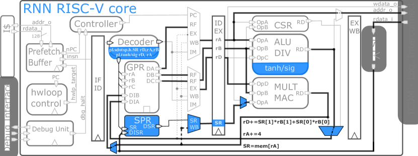
Figure 1: RNN RISC-V Core with extensions to RI5CY core [32] in blue and datapath for pl.sdotpsp instruction marked in bold.

Sigmoid and hyperbolic tangent are common activation functions in neural networks and used in LSTMs. The piecewise linear approximation technique can be implemented for these functions in SW with an increasing number of cycles to reach the required precision. This can be a major contribution to the overall calculation in LSTM-based networks. For example, the calculation of tanh/sig requires 10.3% in [13] and 33.6% in [14] of the overall computation cycles. We introduce two single-cycle instructions pl.tanh rD, rA and pl.sig rD, rA with the following useful properties:

1. They are continuous and smooth (i.e., derivatives are continuous, too); thus, the error is bound for a fixed interval in a Taylor series expansion even for degree one (i.e., $tanh(x_{0}+\epsilon)=tanh(x_{0})+tanh^{\prime}(x_{0})\cdot\epsilon$).

2. The functions converge fast to either $0,1$ or $-1$. Interpolation is needed only on this limited range of numbers.

3. Both functions are symmetric around 0 (i.e., $tanh(-x)=-tanh(x)$ and $sig(-x)=1-sig(x)$), thus just the positive number range needs to be interpolated and the negative range can be derived from the positive values.

Alg. 2 shows the pseudo-code that was used for the hardware implementation of the proposed interpolation. First, we chose the number of intervals of $M$ and the size of every interval $2^{N}$, whereas the interpolation range is $\pm M\cdot 2^{N}$. For both functions $f\in\{tanh,sig\}$ two $M$-entry LUTs $\text{lut\_m}_{f}[\cdot]$ and $\text{lut\_q}_{f}[\cdot]$ are defined. Then the absolute value is calculated (line 2) and the index is calculated by a right shift of the absolute value by $N$ places, if the result is larger than $M$, it is considered to be in the convergence area and either $\{-1,0,1\}$ is returned. Otherwise, the value is calculated by linear approximation within the selected interval id (line 8), sign inverted for negative values (line 9) and subtracted from 1 for negative values in the sigmoid case (l. 10).

Algorithm 2 Pseudocode of the sig and tanh Interpolation

0:  value $x$ and function $f\in{tanh(\cdot),sig(\cdot)}$, interval size $2^{N}$ and #intervals M

1:  

2:  $|x|=\left\{\begin{array}[]{ll}-x&sgn(x)=1\\ x&sgn(x)=-1\end{array}\right.$

3:  $id=|x|>>N$

4:  if id$>$M then

5:     return  $\left\{\begin{array}[]{ll}1&sgn(x)=-1\\ 0&sgn(x)=1,f=sig\\ -1&sgn(x)=1,f=tanh\\ \end{array}\right.$

6:  else

7:     (m,q)=(lut_m_f[id], lut_q_f[id])

8:     $y=m|x|+q$

9:     $y=\left\{\begin{array}[]{ll}-y&sgn(x)=1\\ y&sgn(x)=-1\end{array}\right.$

10:     return  $\left\{\begin{array}[]{ll}1-y&f=sig,\text{sgn}(x)=-1\\ y&\text{else}\\ \end{array}\right.$

11:  end if

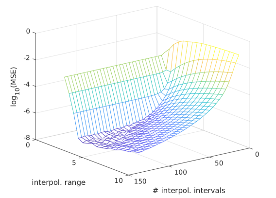
Figure 2: tanh Mean Square Error for different interpolation ranges and number of intervals and $Q_{3.12}$ quantization.

We evaluate the proposed piecewise linear approximation with different number of intervals $2^{N}$ and interpolation ranges, taking into account that fixed-point operations using the $Q_{3.12}$ format are used. The result of this evaluation is illustrated in Fig. 2. For the actual implementation, we have selected an interpolation range of $[-4,4]$ and $2^{5}=32$ intervals, which produces an MSE of $9.81\cdot 10^{-7}$ and a maximum error of $\pm 3.8\cdot 10^{-4}$ when compared to the full-precision hyperbolic tangent function. Evaluation of the quantized RNN benchmarks shows no deterioration of the end-to-end-error when replacing the activation function with our proposed interpolation, which is not surprising as Neural Networks are known to be robust against noise. This extensions reduce the cycle count from 51.2 to 44.5 kcycles within the LSTM networks [13, 14], resulting in a 13.0% improvement.

Figure 3: Speedup with respect to the RISC-V IMC baseline implementation for a typical Neural Networks workload in RRM.

III-E Load and Compute VLIW instruction (HW)

Analyzing the cycle counts in Tab. Ic, we can see that, the lw! and pl.sdotsp.h instructions dominate. By introducing a new instruction, which combines these two within a single pl.sdotsp.h instruction which calculates a 16-bit packed SIMD sum-dot-product:
rD[31:0]+=rA[31:16]*rB[31:16]+ rA[15:0]*rB[15:0]
but also loads data from the memory.

TABLE II: Assembly Code comparison with FM tiling only and with the pl.sdotsp.h instruction

1: 2: 3: 4: 5: 6: 7: 8: 9: 10: 11: 12: 13:	lp.setupi 0, 9, 32 // do {       lw rB, Imm(rBAddr!)       lw rA0, Imm(rAAddr0!)       lw rA1, Imm(rAAddr1!)       lw rA2, Imm(rAAddr2!)       lw rA3, Imm(rAAddr3!)       pv.sdotsp.h rD0, rA0, rB       pv.sdotsp.h rD1, rA1, rB       pv.sdotsp.h rD2, rA2, rB       pv.sdotsp.h rD3, rA3, rB //}	pl.sdotsp.h.0 r0, rA0, r0 pl.sdotsp.h.1 r0, rA1, r0 lp.setupi 0, 5, 32 // do {       lw rB, Imm(rBAddr!) // bubble rB dependency       pl.sdotsp.h.0 rD0, rA2, rB       pl.sdotsp.h.1 rD1, rA3, rB       pl.sdotsp.h.0 rD2, rA0, rB       pl.sdotsp.h.1 rD3, rA1, rB //}

Fig. 1 shows the RI5CY core with the extended datapath of the pl.sdotsp.h instruction with the changes highlighted in colors and its active data paths in bold. rA contains the memory address, loaded from memory by the load/store unit LSU and is incremented for the next data access (i.e., next weight of the corresponding output channel). To avoid a 2-cycle latency, and thus unnecessary stalling, the data is stored in two special-purpose registers SPR and is written and read in an alternating way (using pl.sdotsp.h.0 and pl.sdotsp.h.1 instructions) from these two registers. The data from the SPR is multiplexed as 2nd operand OpA to the multiplier calculating the sum-dot-product. Data hazards are avoided by stalling the pipeline in case of missing grant from memory, exploiting exactly the same signals and control strategy used for standard load words.

Tab. II shows the assembly with output FM tiles of four with (right) and without (left) the extension. In lines 1-2, the SPRs are pre-loaded with the first two weights before the actual main loop. The input FM is loaded in line 4, which is used for the following MAC computation. As can be seen in Tab. Id, the cycle count can effectively be reduced by 1.7$\times$.

Due to the latency of the load word and the dependency with the following instructions, a bubble is inserted in line 5. This can be further optimized by loading two input data (= four input channels), and the result calculated for all the output channels doubling the number of pl.sdotsp.h in the most inner-loop. However, the gains, as seen in Tab. Ie, are rather modest 1.05$\times$ (or 4.9%) since loads and stores from the stack increase by 1.4$\times$ as more registers are needed.

Fig. 3 shows the relative benefits to the RI5CY baseline compared to the output FM tiling, using the instruction extensions and the Input FM Tiling, where for most of the networks the input FM tiling has a positive effect, but few networks (i.e., NNs with small feature sizes) even need more cycles due to the increased stack operations.

IV Core Implementation Results

The extended RI5CY core was implemented in Globalfoundries 22 nm FDX technology using an 8-track low-threshold (LVT) standard cell library and has been synthesized with Synopsys Design Compiler 18.06, back-end flow has been done with Cadence Innovus 18.11 and power estimates are obtained by running gate-level simulations using Modelsim Questa v2019.1 with back-annotated delays from the final layout. When compared to a standard RI5CY core (RV32-IMCXpulp), the new instructions result in a very small circuit area overhead of 2.3 kGE (or 3.4 % of the core area). Furthermore, the critical path of the core remains unchanged (between the load-store unit and the memory in the write-back stage), and the core operates at 380 MHz at 0.65 V at typical conditions at room temperature .

When compared in the same core performing the RISC-V standard RV32-IMC instructions, when executing relevant RNN benchmarks, the enhanced core is on average 15$\times$ faster. It performs 566 MMAC/s (instead of 21 MMAC/s). When the core is using the extensions, the power consumption rises from 1.73 mW to 2.61 mW (51% total increase). While the decoder contributes little more power ($\approx$5µW), the higher power consumption is mainly due to the higher utilization of the compute units (ALU and MAC unit, i.e., 0.57 mW/33% of the total power), the increased GPR usage (0.16 mW/9%), and the higher use of the load-store unit (0.05 mW/3%). However, the overall energy efficiency at 218 GMAC/s/W shows a 10$\times$ improvement.

V Conclusion

We present the first RISC-V core design optimized for RRM applications using machine learning approaches based on RNNs. The core achieves an order-of-magnitude performance (15$\times$) and energy efficiency (10$\times$) improvements over the baseline RISC-V ISA on a wide range or RNN flavors used in RNN. These results are obtained thanks to a synergistic combination of software and hardware optimizations, which only marginally increase area cost and do not affect operating frequency. It is essential to notice that the proposed optimization does not impact numerical precision. Hence labor-intensive quantization-aware retraining is not needed. The enhanced RISC-V core achieves 566 MMAC/s and 218 GMAC/s/W (on 16-bit data types) in 22 nm FDX technology at 0.65 V, thereby providing a fully programmable and efficient open-source IP for future systems-on-chip for 5G Radio Resource Management.

VI Acknowledgments

This work was funded by Huawei Technologies Sweden AB. The authors would like to thank the PULP community for providing a comprehensive and open-source RISC-V platform.

References

- [1] N. D. Tripathi, J. H. Reed, and H. F. VanLandingham, Radio resource management in cellular systems. Springer Science & Business Media, 2006, vol. 618.
- [2] H. Sun, X. Chen, Q. Shi, M. Hong, X. Fu, and N. D. Sidiropoulos, “Learning to optimize: Training deep neural networks for wireless resource management,” in 2017 IEEE 18th International Workshop on Signal Processing Advances in Wireless Communications (SPAWC). IEEE, 7 2017, pp. 1–6. [Online]. Available: http://ieeexplore.ieee.org/document/8227766/
- [3] K. I. Ahmed, H. Tabassum, and E. Hossain, “Deep Learning for Radio Resource Allocation in Multi-Cell Networks,” IEEE Network, 8 2019. [Online]. Available: http://arxiv.org/abs/1808.00667
- [4] Q. Shi, M. Razaviyayn, Z.-Q. Luo, and C. He, “An iteratively weighted MMSE approach to distributed sum-utility maximization for a MIMO interfering broadcast channel,” in Acoustics, Speech and Signal Processing (ICASSP), 2011 IEEE International Conference on. IEEE, 2011, pp. 3060–3063.
- [5] M. Naeem, K. Illanko, A. Karmokar, A. Anpalagan, and M. Jaseemuddin, “Optimal power allocation for green cognitive radio: fractional programming approach,” IET Communications, vol. 7, no. 12, pp. 1279–1286, 2013.
- [6] M. Yao, M. M. Sohul, X. Ma, V. Marojevic, and J. H. Reed, “Sustainable green networking: exploiting degrees of freedom towards energy-efficient 5G systems,” Wireless Networks, vol. 25, no. 3, pp. 951–960, 4 2019. [Online]. Available: http://link.springer.com/10.1007/s11276-017-1626-7
- [7] M. Yao, M. Sohul, V. Marojevic, and J. H. Reed, “Artificial Intelligence Defined 5G Radio Access Networks,” IEEE Communications Magazine, vol. 57, no. 3, pp. 14–20, 2019.
- [8] X. Ge, S. Tu, G. Mao, C.-X. Wang, and T. Han, “5G ultra-dense cellular networks,” IEEE Wireless Communications, vol. 23, no. 1, pp. 72–79, 2016.
- [9] H. Ye and G. Y. Li, “Deep reinforcement learning for resource allocation in V2V communications,” in 2018 IEEE International Conference on Communications (ICC). IEEE, 2018, pp. 1–6. [Online]. Available: https://ieeexplore.ieee.org/abstract/document/8422586/
- [10] E. Ghadimi, F. Davide Calabrese, G. Peters, and P. Soldati, “A reinforcement learning approach to power control and rate adaptation in cellular networks,” in 2017 IEEE International Conference on Communications (ICC). IEEE, 5 2017, pp. 1–7. [Online]. Available: http://ieeexplore.ieee.org/document/7997440/
- [11] Y. Yu, T. Wang, and S. C. Liew, “Deep-reinforcement learning multiple access for heterogeneous wireless networks,” ieeexplore.ieee.org, 11 2017. [Online]. Available: https://ieeexplore.ieee.org/abstract/document/8422168/similar%****␣rnn_at_Arxiv.bbl␣Line␣100␣****http://arxiv.org/abs/1712.00162
- [12] Y. S. Nasir and D. Guo, “Deep Reinforcement Learning for Distributed Dynamic Power Allocation in Wireless Networks,” 8 2018. [Online]. Available: http://arxiv.org/abs/1808.00490
- [13] U. Challita, L. Dong, and W. Saad, “Proactive Resource Management in LTE-U Systems: A Deep Learning Perspective,” 2 2017. [Online]. Available: http://arxiv.org/abs/1702.07031
- [14] O. Naparstek and K. Cohen, “Deep Multi-User Reinforcement Learning for Distributed Dynamic Spectrum Access,” IEEE Transactions on Wireless Communications, vol. 18, no. 1, pp. 310–323, 4 2019. [Online]. Available: http://arxiv.org/abs/1704.02613
- [15] W. Lee, M. Kim, and D.-H. Cho, “Deep Power Control: Transmit Power Control Scheme Based on Convolutional Neural Network,” IEEE Communications Letters, vol. 22, no. 6, pp. 1276–1279, 6 2018. [Online]. Available: https://ieeexplore.ieee.org/document/8335785/
- [16] Mnih Volodymyr, et al., V. Mnih, K. Kavukcuoglu, D. Silver, A. A. Rusu, J. Veness, M. G. Bellemare, A. Graves, M. Riedmiller, A. K. Fidjeland, G. Ostrovski, S. Petersen, C. Beattie, A. Sadik, I. Antonoglou, H. King, D. Kumaran, D. Wierstra, S. Legg, and D. Hassabis, “Human-level control through deep reinforcement learning,” Nature, vol. 518, no. 7540, pp. 529–33, 2 2015. [Online]. Available: http://www.ncbi.nlm.nih.gov/pubmed/25719670
- [17] S. Wang, H. Liu, P. H. Gomes, and B. Krishnamachari, “Deep reinforcement learning for dynamic multichannel access in wireless networks,” IEEE Transactions on Cognitive Communications and Networking, 2018.
- [18] A. Reuther, P. Michaleas, M. Jones, V. Gadepally, S. Samsi, and J. Kepner, “Survey and Benchmarking of Machine Learning Accelerators,” arXiv preprint arXiv:1908.11348, 2019.
- [19] S. Cao, C. Zhang, Z. Yao, W. Xiao, L. Nie, D. Zhan, Y. Liu, M. Wu, and L. Zhang, “Efficient and Effective Sparse LSTM on FPGA with Bank-Balanced Sparsity,” in Proceedings of the 2019 ACM/SIGDA International Symposium on Field-Programmable Gate Arrays, ser. FPGA ’19. New York, NY, USA: ACM, 2019, pp. 63–72. [Online]. Available: http://doi.acm.org/10.1145/3289602.3293898
- [20] C. Gao, D. Neil, E. Ceolini, S.-C. Liu, and T. Delbruck, “DeltaRNN: A power-efficient recurrent neural network accelerator,” in Proceedings of the 2018 ACM/SIGDA International Symposium on Field-Programmable Gate Arrays. ACM, 2018, pp. 21–30.
- [21] Intel Corp., “Intel® Architecture Instruction Set Extensions and Future Features Programming Reference,” 2019.
- [22] J. Yiu, “Introduction to Armv8.1-M architecture,” ARM, no. February, pp. 1–14, 2019.
- [23] L. Lai, N. Suda, and V. Chandra, “Cmsis-nn: Efficient neural network kernels for arm cortex-m cpus,” arXiv preprint arXiv:1801.06601, 2018.
- [24] A. Garofalo, M. Rusci, F. Conti, D. Rossi, and L. Benini, “PULP-NN: accelerating quantized neural networks on parallel ultra-low-power RISC-V processors,” Philosophical Transactions of the Royal Society A, vol. 378, no. 2164, p. 20190155, 2020.
- [25] K. Chellapilla, S. Puri, and P. Simard, “High performance convolutional neural networks for document processing,” in Tenth International Workshop on Frontiers in Handwriting Recognition, 2006.
- [26] D. Lin, S. Talathi, and S. Annapureddy, “Fixed point quantization of deep convolutional networks,” in International Conference on Machine Learning, 2016, pp. 2849–2858.
- [27] B. Jacob, S. Kligys, B. Chen, M. Zhu, M. Tang, A. Howard, H. Adam, and D. Kalenichenko, “Quantization and training of neural networks for efficient integer-arithmetic-only inference,” in Proceedings of the IEEE Conference on Computer Vision and Pattern Recognition, 2018, pp. 2704–2713.
- [28] C.-W. Lin and J.-S. Wang, “A digital circuit design of hyperbolic tangent sigmoid function for neural networks,” in 2008 IEEE International Symposium on Circuits and Systems. IEEE, 2008, pp. 856–859.
- [29] K. Leboeuf, A. H. Namin, R. Muscedere, H. Wu, and M. Ahmadi, “High speed VLSI implementation of the hyperbolic tangent sigmoid function,” in 2008 Third International Conference on Convergence and Hybrid Information Technology, vol. 1. IEEE, 2008, pp. 1070–1073.
- [30] C.-H. Tsai, Y.-T. Chih, W. H. Wong, and C.-Y. Lee, “A hardware-efficient sigmoid function with adjustable precision for a neural network system,” IEEE Transactions on Circuits and Systems II: Express Briefs, vol. 62, no. 11, pp. 1073–1077, 2015.
- [31] A. Waterman, Y. Lee, D. A. Patterson, and K. Asanovi, “The RISC-V Instruction Set Manual. Volume 1: User-Level ISA, Version 2.0,” CALIFORNIA UNIV BERKELEY DEPT OF ELECTRICAL ENGINEERING AND COMPUTER SCIENCES, Tech. Rep., 2014.
- [32] M. Gautschi, P. D. Schiavone, A. Traber, I. Loi, A. Pullini, D. Rossi, E. Flamand, F. K. Gürkaynak, and L. Benini, “Near-Threshold RISC-V core with DSP extensions for scalable IoT endpoint devices,” IEEE TVLSI, vol. 25, no. 10, pp. 2700–2713, 2017.
- [33] M. Eisen, C. Zhang, L. F. Chamon, D. D. Lee, and A. Ribeiro, “Learning Optimal Resource Allocations in Wireless Systems,” IEEE Transactions on Signal Processing, vol. 67, no. 10, pp. 2775–2790, 2019. [Online]. Available: https://arxiv.org/abs/1807.08088
- [34] R. Andri, T. Henriksson, and L. Benini, “RNN Acceleration Extension for RISC-V Project Report I,” https://github.com/andrire/RNNASIP/blob/7c9b8e7/docs/Report1/ report.pdf, 2019.