Dynamical perturbation theory for eigenvalue problems

Abstract

Many problems in physics, chemistry and other fields are perturbative in nature, i.e. differ only slightly from related problems with known solutions. Prominent among these is the eigenvalue perturbation problem, wherein one seeks the eigenvectors and eigenvalues of a matrix with small off-diagonal elements. Here we introduce a novel iterative algorithm to compute these eigenpairs based on fixed-point iteration for an algebraic equation in complex projective space. We show from explicit and numerical examples that our algorithm outperforms the usual Rayleigh-Schrödinger expansion on three counts. First, since it is not defined as a power series, its domain of convergence is not a priori confined to a disk in the complex plane; we find that it indeed usually extends beyond the standard perturbative radius of convergence. Second, it converges at a faster rate than the Rayleigh-Schrödinger expansion, i.e. fewer iterations are required to reach a given precision. Third, the (time- and space-) algorithmic complexity of each iteration does not increase with the order of the approximation, allowing for higher precision computations. Because this complexity is merely that of matrix multiplication, our dynamical scheme also scales better with the size of the matrix than general-purpose eigenvalue routines such as the shifted QR or divide-and-conquer algorithms. Whether they are dense, sparse, symmetric or unsymmetric, we confirm that dynamical diagonalization quickly outpaces LAPACK drivers as the size of matrices grows; for the computation of just the dominant eigenvector, our method converges order of magnitudes faster than the Arnoldi algorithm implemented in ARPACK.

I Introduction

Computing the eigenvalues and eigenvectors of a matrix that is already close to being diagonal (or diagonalizable in a known basis) is a central problem in many branches of applied mathematics. The standard approach, outlined a century ago by Rayleigh Rayleigh (1894) and Schrödinger Schrödinger (1926), consists in assuming a power series in a perturbation parameter $\lambda$ and extracting the coefficients order by order from the eigenvalue equation. Historically, this technique played a central role in the development of quantum mechanics, providing analytical insight into e.g. level splitting in external fields Schrödinger (1926), radiative corrections Bethe (1947) or localization in disordered systems Anderson (1958). Suitably adapted to the problem at hand Møller and Plesset (1934); Epstein (1926); Nesbet (1955), Rayleigh-Schrödinger (RS) perturbation theory remains the workhorse of many ab initio calculations in quantum many-body theory Szabo and Ostlund (1989) and quantum field theory Zuber and Itzykson (2006). Outside the physical sciences, RS perturbation theory underlies the quasispecies theory of molecular evolution Eigen et al. (1988), among countless other applications.

The shortcomings of the RS series are well known. First, its explicit form requires that all unperturbed eigenvalues be simple, else the perturbation must first be diagonalized in the degenerate eigenspace through some other method. Second, the number of terms to evaluate grows with the order of the approximation; to keep track of them, cumbersome diagrammatic techniques are often required. Third, the RS series may not converge for all (or, in infinite dimensions, any) values of $\lambda$ Dyson (1952); Kato (1966); Simon (1991). Indeed, since the RS series is a power series, its domain of convergence is confined to a disk in the complex $\lambda$-plane: if a singularity exists at location $\lambda_{*}$, then the RS series will necessarily diverge for any value $\lambda$ such that $|\lambda|>|\lambda_{*}|$. This means that a non-physical (e.g. imaginary) singularity can contaminate the RS expansion, turning it into a divergent series in regions where the spectrum is, in fact, analytic. Of course, divergent power series can still be useful: the partial sums often approaches the solution rather closely before blowing up; what is more, a wealth of resummation techniques, such as Borel resummation or Padé approximants, can be used to extract convergent approximations from the coefficients Janke and Kleinert (2007).

In this paper we introduce an explicit perturbation scheme for finite-dimensional (Hermitian or non-Hermitian) eigenvalue problems alternative to the RS expansion. Instead of assuming a power series in $\lambda$, we build a sequence of approximations of the eigenpairs by iterating a non-linear map in matrix space, i.e. through a discrete-time dynamical system. As we will see, this alternative formulation of perturbation theory compares favorably with the conventional RS series—which can be recovered through truncation—with regards to the second (complexity) and third (convergence) points above. Our novel scheme is also surprisingly fast from a computational viewpoint, offering an efficient alternative to standard diagonalization algorithms for large perturbative matrices.

Our presentation combines theoretical results with numerical evidence. We prove that (i) our dynamical scheme reduces to the RS partial sum when truncated to $\mathcal{O}(\lambda^{k})$, and (ii) there exists a neighborhood of $\lambda=0$ where it converges exponentially to the full set of perturbed eigenvectors. The latter result is analogous to Kato’s lower bound on the radius of convergence of RS perturbation theory Kato (1966); like the latter, it provides sufficient but not necessary conditions for convergence at finite $\lambda$. To illustrate the performance of our algorithm, we analyze several examples of perturbative matrix families, including a quantum harmonic oscillator perturbed by a $\delta$-potential and various ensembles of (dense and sparse) random perturbations.

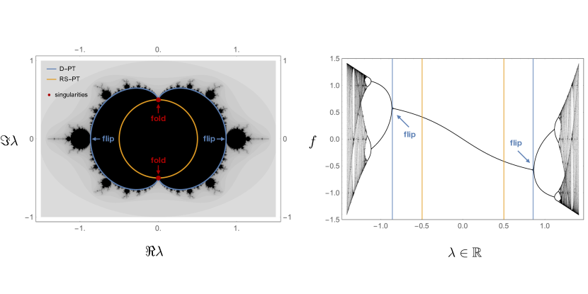
Figure 1: Convergence of perturbation theory in the two-dimensional example (5). Left: In the complex $\lambda$-plane, RS perturbation theory (RS-PT) converges inside a circle of radius $1/2$ (orange line) bounded by the exceptional points $\pm i/2$ where eigenvalues have branch-point singularities and $M$ is not diagonalizable. Dynamical perturbation theory (D-PT) converges inside the domain bounded by the blue cardioid, which is larger—especially along the real axis, where there is no singularity. Outside this domain, the map can converge to a periodic cycle, be chaotic or diverge to infinity, following flip bifurcations (along the real axis) and fold bifurcations (at the singularities). The domain where the map remains bounded (black area) is a conformal transformation of the Mandelbrot set. Right: The bifurcation diagram for the quadratic map $f$ along the real $\lambda$-axis illustrates the period-doubling route to chaos as $\lambda$ increases away from $0$ (in absolute value). Orange and left vertical lines indicate the boundary of the convergence domains of RS-PT and D-PT respectively. 

II Results

II.1 Eigenvectors as affine variety

We begin with the observation that, being defined up to a multiplicative constant, the eigenvectors of an $N\times N$ matrix $M$ are naturally viewed as elements of the complex projective space $\mathbb{C}P^{N-1}$. Let $[x^{1}\,:\,\cdots\,:\,x^{N}]$ denote the homogeneous coordinates of $x\in\mathbb{C}P^{N-1}$. Fix an index $1\leq n\leq N$, and consider an eigenvector $z_{n}$ of $M$ such that $z_{n}^{\,n}\neq 0$. From the eigenvalue equation $Mz_{n}=\varepsilon_{n}z_{n}$ we can extract the eigenvalue as $\varepsilon_{n}=(Mz_{n})^{n}/z_{n}^{\,n}$; inserting this back into $Mz_{n}=\varepsilon_{n}z_{n}$ shows that $z_{n}$ is a projective root of the system of $N-1$ homogeneous quadratic equations

$$(Mz_{n})^{m}z_{n}^{\,n}=(Mz_{n})^{n}z_{n}^{\,m}\quad\textrm{for}\quad m\neq n.$$

Denoting $V_{n}$ the projective variety defined by these equations and $U_{n}$ the affine chart in which the $n$-th homogeneous coordinate is nonzero, we arrive at the conclusion that the set of eigenvectors of $M$ is the affine variety $\cup_{n}(V_{n}\cap U_{n})$, see SI.1 for details. Since eigenvectors generically have non-zero coordinates in all directions, each one of $V_{n}\cap U_{n}$ normally contains the complete set of eigenvectors.

II.2 Eigenvectors as fixed points

We now further assume a perturbative partioning $M=D+\lambda\Delta,$ where the diagonal part $D$ consists of unperturbed eigenvalues $\epsilon_{n}$ and $\lambda\Delta$ is a perturbation parametrized by $\lambda\in\mathbb{C}$. Provided the $\epsilon_{n}$’s are all simple (non-degenerate), we can rewrite the polynomial system above as

$$z_{n}^{\,n}z_{n}^{\,m}=\lambda\theta_{n}^{\,m}\left(z_{n}^{\,n}(\Delta z_{n})^{m}-z_{n}^{\,m}(\Delta z_{n})^{n}\right)\quad\textrm{for}\quad m\neq n,$$

where $\theta_{n}^{\,m}\equiv(\epsilon_{n}-\epsilon_{m})^{-1}$. Within the chart $U_{n}$ we are free to set $z_{n}^{\,n}=1$; this results in the fixed point equation $z_{n}=F_{n}(z_{n})$ with $F_{n}:U_{n}\to U_{n}$ the map with components

$$F_{n}^{\,m}(z_{n})\equiv\delta_{n}^{\,m}+\lambda\theta_{n}^{\,m}\left((\Delta z_{n})^{m}-(\Delta z_{n})^{n}z_{n}^{\,m}\right)\quad\textrm{for}\quad 1\leq m\leq N,$$ (1)

where the matrix $\theta$ is completed with $\theta_{n}^{\,n}=0$ and $\delta_{n}^{\,m}$ are the components of the unit matrix $I$.

As noted above, each one of these maps $F_{n}:U_{n}\to U_{n}$ generically has the full set of eigenvectors of $M$ as fixed points. Here, however, we wish to compute these fixed points dynamically, as limits of the iterated map

$$z_{n}^{(k+1)}=F_{n}(z_{n}^{(k)}).$$

For this procedure to converge, the map $F_{n}$ must be contracting in the neighborhood of at least one fixed point; for small $\lambda$ this is always the case for the fixed point closest to the unperturbed eigenvector $e_{n}\equiv(\delta_{n}^{\,m})_{1\leq m\leq N}$, but usually not for the other fixed points. To compute all the eigenvectors of $M$, we must therefore iterate not one, but all the maps $F_{n}$ together, ideally in parallel.

We can achieve this by bundling all $N$candidate eigenvectors in a list and applying the map $F_{n}$ to the $n$-th component:

$$F:\prod_{1\leq n\leq N}U_{n} \longrightarrow\prod_{1\leq n\leq N}U_{n}$$

$$(z_{1},\cdots,z_{N}) \longmapsto(F_{1}(z_{1}),\cdots,F_{N}(z_{N}))$$

Introducing the matrix $A$ whose $n$-th line is the vector $z_{n}$, this can be written in matrix form as

$$F(A)=I+\lambda\theta\star\left(A\Delta^{\prime}-(A\Delta^{\prime})\triangleright A\right).$$ (2)

Here prime denotes the transpose, $\star$ the Hadamard (element-wise) product of matrices, and $A\triangleright B\equiv(I\star A)B$. The dynamical system in the title is then obtained through iterated applications of $F$ to the identity matrix of unperturbed eigenvectors $I$, generating the sequence of approximating eigenvectors

$$A_{\textrm{D}}^{(k)}=F(A_{\textrm{D}}^{(k-1)})=\cdots=F^{\circ k}(I).$$ (3)

The eigenvalues $\varepsilon^{(k)}_{n}$ at order $k$ are given by $\varepsilon_{n}^{(k)}=\epsilon_{n}+(A_{\textrm{D}}^{(k)}\Delta^{\prime})_{n}^{\,n}$.

II.3 Convergence at small $\lambda$

It is not hard show that $A_{\textrm{D}}^{(k)}$ always converges at small $\lambda$. Let $\|\cdot\|$ denote the spectral norm of matrices (the largest singular value), which is sub-multiplicative with respect to both the matrix and Hadamard products Horn and Johnson (2012), and assume $\|\Delta\|=1$ without loss of generality. First, $\|F(A)-I\|\leq\|\lambda\theta\|(\|A\|+\|A\|^{2})$ implies that $F$ maps a closed ball $B_{r}(I)$ of radius $r$ centered on $I$ onto itself whenever $\|\lambda\theta\|\leq r/[(1+r)(2+r)]$.  Next, from (2) we have

$$\|F(A)-F(B)\|\leq\|\lambda\theta\|\,(1+\|A+B\|)\,\|A-B\|.$$

Hence, $F$ is contracting in $B_{r}(I)$ provided $\|\lambda\theta\|<1/[1+2(1+r)]$. Under these conditions the Banach fixed-point theorem implies that $A_{\textrm{D}}^{(k)}=F^{\circ k}(I)$ converges exponentially to a unique fixed point within this ball as $k\to\infty$. Choosing the optimal radius

$$\underset{r>0}{\textrm{argmax}}\min\,\left(\frac{r}{(1+r)(2+r)},\frac{1}{1+2(1+r)}\right)=\sqrt{2},$$

we see that $|\lambda|<(3-2\sqrt{2})\|\theta\|^{-1}\approx 0.17\|\theta\|^{-1}$ guarantees convergence to the fixed point.

II.4 Contrast with RS perturbation theory

Let us now contrast this iterative method with conventional RS perturbation theory. There, the eigenvectors of $M$ are sought as power series in $\lambda$, viz. $z=\sum_{\ell}z^{(\ell)}\lambda^{\ell}$. Identifying the terms of the same order in $\lambda$ in the eigenvalue equation, one obtains for the matrix of eigenvectors at order $k$

$$A^{(k)}_{\textrm{RS}}=\sum_{\ell=0}^{k}a^{(\ell)}\lambda^{\ell}$$

in which the matrix coefficients $a^{(\ell)}$ are obtained from $a^{(0)}=I$ via the recursion (SI.2)

$$a^{(\ell)}=\theta\star\left(a^{(\ell-1)}\Delta^{\prime}-\sum_{s=0}^{\ell-1}(a^{(s)}\Delta^{\prime})\triangleright a^{(\ell-1-s)}\right).$$ (4)

We show in SI.3 that the dynamical scheme $A^{(k)}_{\textrm{D}}$ completely contains this RS series, in the sense that $A^{(k)}_{\textrm{D}}=A^{(k)}_{\textrm{RS}}+\mathcal{O}(\lambda^{k+1}).$ For example, to order $2$ we have

$$A^{(2)}_{\textrm{RS}}=I+\lambda\theta\star\Delta^{\prime}+\lambda^{2}\theta\star\Big{(}(\theta\star\Delta^{\prime})\Delta^{\prime}\Big{)},$$

and

$$A^{(2)}_{\textrm{D}}=A^{(2)}_{\textrm{RS}}+\lambda^{3}\theta\star\Big{[}\Big{(}(\theta\star\Delta^{\prime})\Delta^{\prime}\Big{)}\triangleright(\theta\star\Delta^{\prime})\Big{]}.$$

This means that we can recover the usual perturbative expansion of $A$ to order $k$ by iterating $k$ times the map $F$ and dropping all terms $\mathcal{O}(\lambda^{k+1})$. Moreover, the parameter whose smallness determines the convergence of the RS series is the product of the perturbation magnitude $\lambda$ with the inverse diagonal gaps $\theta$ Kato (1966), just as it determines the contraction property of $F$.

These similarities notwithstanding, the dynamical scheme differs from the RS series in two key ways. First, the complexity of each iteration is constant (one matrix product with $\Delta^{\prime}$ and one Hadamard product with $\theta$, which is faster), whereas computing the RS coefficients $a^{(\ell)}$ involves the sum of increasingly many matrix products. Second, not being defined as a power series, the convergence of $A^{(k)}_{\textrm{D}}$ when $k\to\infty$ is not a priori restricted to a disk in the complex $\lambda$-plane. Together, these two differences suggest that our dynamical scheme has the potential to converge faster, and in a larger domain, than RS perturbation theory. This is what we now examine, starting from an elementary but explicit example.

II.5 An explicit $2\times 2$ example

Consider the symmetric matrix

$$M=\begin{pmatrix}0&0\\ 0&1\end{pmatrix}+\lambda\begin{pmatrix}0&1\\ 1&0\end{pmatrix}.$$ (5)

This matrix has eigenvalues $\varepsilon_{\pm}=(1\pm\sqrt{1+4\lambda^{2}})/2$, both of which are analytic inside the disk $|\lambda|<1/2$ but have branch-point singularities at $\lambda=\pm i/2$. (These singularities are in fact exceptional points, i.e. $M$ is not diagonalizable for these values.) Because the RS series is a power series, these imaginary points contaminate its convergence also on the real axis, where no singularity exists: $A_{\textrm{RS}}$ diverges for any value of $\lambda$ outside the disk of radius $1/2$, and in particular for real $\lambda>1/2$ .

Considering instead our iterative scheme, one easily computes

$$A^{(k)}_{\textrm{D}}=\begin{pmatrix}1&f^{\circ k}(0)\\ -f^{\circ k}(0)&1\end{pmatrix},$$

where $f(x)=\lambda(x^{2}-1)$ and the superscripts indicate $k$-fold iterates. This one-dimensional map has two fixed points at $x^{*}_{\pm}=\varepsilon_{\pm}/\lambda$. Of these two fixed points $x^{*}_{+}$ is always unstable, while $x^{*}_{-}$ is stable for $\lambda\in(-\sqrt{3}/2,\sqrt{3}/2)$ and loses its stability at $\lambda=\pm\sqrt{3}/2$ in a flip bifurcation. At yet larger values of $\lambda$, the iterated map $f^{\circ k}$—hence the fixed-point iterations $A^{(k)}_{\textrm{D}}$—follows the period-doubling route to chaos familiar from the logistic map May (1976). For values of $\lambda$ along the imaginary axis, we find that the map is stable if $\Im\lambda\in(-1/2,1/2)$ and loses stability in a fold bifurcation at the exceptional points $\lambda=\pm i/2$. The full domain of convergence of the system is strictly larger than the RS disk, as shown in Fig. 1. Further details on the algebraic curve bounding this domain are given in SI.4-.5.

We also observe that the disk where both schemes converge, the dynamical scheme does so with a better rate than RS perturbation theory: we check that $|f^{\circ k}(0)-x^{*}_{-}|\sim|1-\sqrt{1+4\lambda^{2}}|^{k}=\mathcal{O}(|2\lambda^{2}|^{k})$, while the remainder of the RS decays as $\mathcal{O}(|2\lambda|^{k})$. This is a third way in which the dynamical scheme outperforms the usual RS series, at least in this case: not only is each iteration computationally cheaper, but the number of iterations required to reach a given precision is lower.

II.6 Quantum harmonic oscillator with $\delta$-potential

As a second illustration let us consider the Hamiltonian of a quantum harmonic oscillator perturbed by a $\delta$-potential at the origin,

$$H=\left(-\frac{1}{2}\frac{\partial^{2}}{\partial x^{2}}+\frac{1}{2}x^{2}\right)+\lambda\delta(x),$$ (6)

where the unperturbed Hamiltonian (in brackets) is diagonal in the basis of Hermite functions $\phi_{n}(x)=(2^{n}n!\sqrt{\pi})^{-1/2}H_{n}(x)e^{-x^{2}/2}$ with eigenvalues $\epsilon_{n}=n+1/2$. For this example familiar from elementary quantum mechanics Viana-Gomes and Peres (2011), it was estimated in Kvaal et al. (2011) that the RS series converges for all $|\lambda|<2$. Since (by parity) the perturbation only affects the even-number eigenfunctions, we consider the matrices $D_{n}^{\,m}=(2n+1/2)\delta_{n}^{\,m}$ and $\Delta_{n}^{\,m}=\phi_{2n}(0)\phi_{2m}(0)$ with $n,m$ truncated at some value $N$.

Fig. 2 compares the convergence of the matrix of eigenvectors $A^{(k)}_{\textrm{RS,D}}$ with the order $k$ under the RS and dynamical schemes. While convergence is manifestly  exponential in both cases, the rate is faster in dynamical perturbation theory, particularly at larger values of $\lambda$. For instance, for $\lambda=1.5$ it takes over $70$ orders in conventional perturbation theory to reach the same precision as $\sim 40$ iterations of the map $F$; when $\lambda=2.5$ the RS series no longer converges, but the orbits of (2) still do. In the limit where $N\to\infty$ (the complete quantum mechanical problem) we found that the RS series has a radius of convergence $\approx 2.2$, whereas dynamical perturbation theory converges up to $\lambda_{\textrm{max}}\approx 2.9$.

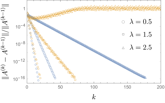
Figure 2: Convergence of the RS perturbative series (RS-PT, orange symbols) and of our dynamical scheme (D-PT, blue symbols) for the perturbed harmonic oscillator in (6) with $N=100$ and increasing values of $\lambda$. The latter converges at a faster rate, and in a larger domain, than the RS series. 

II.7 An improved perturbation theory

These improved convergence properties are not special to the matrix families (5) or (6). To see this, let us now consider an ensemble of (nonsymmetric) random matrices of the form $M=\textrm{diag}(n)_{1\leq n\leq N}+\lambda R$ where $R$ are $N\times N$ arrays of random numbers uniformly distributed between $-1$ and $1$. For given $N$ and $\lambda$, we compute the success rate (probability of convergence) of each method, and, in cases where both converge, the orders $K_{\textrm{D}}$ and $K_{\textrm{RS}}$ required by each to converge at hundred-digit precision.

Fig. 3 plots the difference $K_{\textrm{RS}}-K_{\textrm{D}}$ for matrices of size $N=100$ at various values of $\lambda$. In a large majority of cases (out of $50$ samples for each $\lambda$), the difference turns out positive, implying that dynamical perturbation converges as a faster rate than RS perturbation theory. The success rate (inset) is also better with the former, confirming the patterns observed in the $2\times 2$ and $\delta$-potential examples.

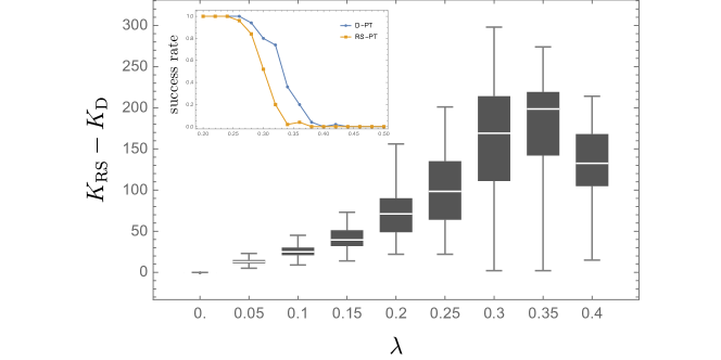
Figure 3: Comparison of the convergence rates of dynamical perturbation theory (D-PT) and RS perturbation theory (RS-PT) for random matrices with $N=100$, equally spaced diagonal entries and uniformly distributed off-diagonal elements. A positive value of $K_{\textrm{RS}}-K_{\textrm{D}}$ indicates that D-PT reaches hundred-digit precision for the full set of eigenvectors with fewer iterations than RS-PT; this is true in a large majority of cases, though not always. The inset shows that D-PT is also more likely to converge (for a given $\lambda$) than RS-PT. 

II.8 A subcubic eigenvalue algorithm

We noted earlier that the algorithmic complexity of each iteration of the map is limited by that of matrix multiplication by $\Delta^{\prime}$. The complexity of matrix multiplication is theoretically $\mathcal{O}(N^{2.37\cdots})$ Coppersmith and Winograd (1990); Gall (2014); the Strassen algorithm Strassen (1969) often used in practice performs in $\mathcal{O}(N^{2.8\cdots})$ or better for sparse matrices. This implies that, within its domain of convergence (i.e. for matrices with small off-diagonal elements), our dynamical scheme scales better than classical diagonalization algorithms such as shifted Hessenberg QR (for nonsymmetric matrices) or divide-and-conquer (for Hermitian matrices), which are all $\mathcal{O}(N^{3})$ if all eigenpairs are requested Demmel (1997).

We tested this premise by comparing the timing of the complete dynamical diagonalization of large matrices with general-purpose LAPACK routines Anderson et al. (1999), implemented in Mathematica 12 in the function Eigensystem. To this aim we considered two classes of random perturbations of the harmonic oscillator in (6): dense nonsymmetric matrices with uniformly distributed entries, and sparse Laplacian (hence symmetric) matrices of critical Erdős-Rényi random graphs (i.e. with $N$ vertices and $N$ edges). The perturbation parameter was set to $\lambda=0.01$ and timings were made both at machine precision and at fixed precision ($p=100$ digits). Finally, we used a partioning of the matrices in which $\Delta$ has vanishing diagonal elements; this partioning is known in quantum chemistry as Epstein-Nesbet perturbation theory Epstein (1926); Nesbet (1955). In each case dynamical perturbation theory proved (much) faster than LAPACK routines at large $N$.

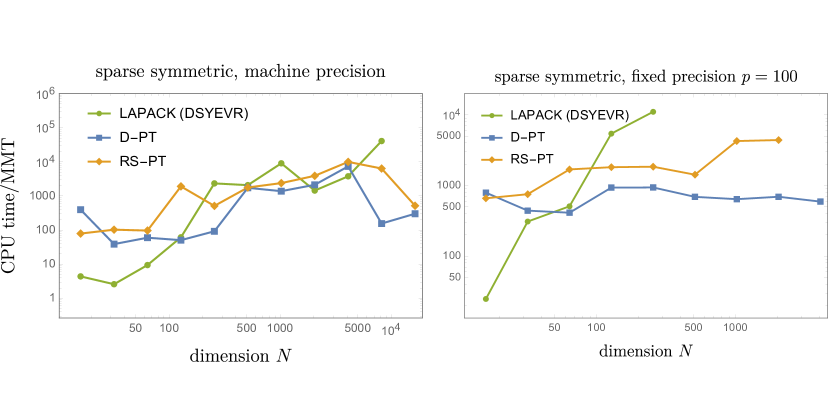
Figure 4: Performance of perturbative (dynamical, D-PT, and Rayleigh-Schrödinger, RS-PT) diagonalization vs. the DSYEVR LAPACK routine (implemented as Eigensystem in Mathematica 12) for sparse symmetric matrices, given as ratios of CPU time to matrix multiplication time (MMT). Unlike standard cubic algorithms, the complexity of our dynamical scheme is just that matrix multiplication.  As a result, D-PT quickly outpaces LAPACK at both machine (left) or—even more impressively—fixed precision (right). The values given are averages over $50$ repetitions with a time constraint of one hour. 

Representative results are given in Fig. 4, where we plot the ratio of the CPU time required to compute all the eigenvectors of sparse $M$ to the CPU time to compute its square $M^{2}$ (matrix multiplication time MMT). While this ratio increases sharply with $N$ with standard algorithms, it does not with our iterative algorithm. As a result, dynamical perturbation theory quickly outperforms LAPACK (here the DSYEVR routine for symmetric matrices), and especially its fixed precision version in Mathematica. The large improvement is remarkable because symmetric eigenvalue solvers are among the best understood, and most fine-tuned, algorithms in numerical mathematics Golub and van der Vorst (2000). Our implementation of (2), on the other hand, was written entirely in Mathematica, i.e. without the benefit of compiled languages.

Finally we considered the computation of just the dominant eigenvector of $M$ (the one with the largest eigenvalue). In contrast with the complete eigenproblem, subcubic algorithms exist for finding such extremal eigenvectors, such as the Arnoldi and Lanczos algorithms or Rayleigh quotient iteration Demmel (1997). Thanks to their iterative nature—similar to our dynamical scheme—these algorithms perform especially well with sparse matrices, and are generally viewed as setting a high bar for computational efficiency. Yet, for sparse perturbative matrices (such that the dominant eigenvector $z_{n^{*}}$ is the one associated with the largest unperturbed eigenvalue $\epsilon_{n^{*}}$), we found that the iteration of the single-vector map $F_{n^{*}}$ converges orders of magnitudes faster than these iterative algorithms (Fig. 5). For instance, it took just $4$ iterations and $3$ seconds on a desktop machine to compute at machine precision the dominant eigenpair of a sparse symmetric matrix with $10^{8}$ non-zero elements ($\sim 1.5$ Go in memory); by contrast ARPACK’s Lanczos algorithm had not converged within a $100$s cutoff for a matrix $50$ times smaller.

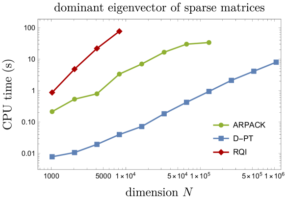
Figure 5: CPU time to compute the dominant eigenvector of sparse perturbative matrices at machine precision with the Lanczos algorithm in Mathematica’s ARPACK routine (with starting vector provided), with the single-vector map (1) (D-PT), and with Reyleigh quotient iteration (RQI). Dynamical perturbation theory is much faster, even in our non-compiled Mathematica implementation. 

Overall, these timings suggest that, although certainly not a general-purpose method due to its limited convergence domain, dynamical diagonalization can be an efficient approach to the numerical eigenvalue problem, whether all eigenpairs are needed (in which case it is pleasantly parallel) or just a few. When the matrix of interest has off-diagonal elements which are not small, it might still be possible to compute approximate eigenvectors through another method (say to $1\%$ accuracy) and improve the performance by using dynamical diagonalization for the final convergent steps.

III Discussion

We reconsidered the classic problem of computing the eigensystem of a matrix given in diagonal form plus a small perturbation. Departing from the usual prescription based on power series expansions, we identified a quadratic map in matrix space whose fixed points are the sought-for eigenvectors, and proposed to compute them through fixed-point iteration, i.e. as a discrete-time  dynamical system. We showed empirically that this algorithm outperforms the usual RS series on three counts: each iteration has lower computational complexity, the rate of convergence is usually higher (so that fewer iterations are needed to reach a given precision), and the domain of convergence of the scheme (with respect to the perturbation parameter $\lambda$) is usually larger. Within its domain of convergence, our algorithm runs much faster than standard exact diagonalization routines because its complexity is merely that of matrix multiplication (by the perturbation $\Delta$).

Several extensions of our method can be considered. For instance, when $\lambda$ is too large and the dynamical system does not converge, we may reduce it to $\lambda/Q$ for some integer $Q$, diagonalize the matrix with this smaller perturbation, restart the algorithm using the diagonal matrix thus obtained as initial condition, and repeat the operation $Q$ times. This approach is similar to the homotopy continuation method for finding polynomial roots Morgan (2009) and can effectively extend the domain of convergence of the dynamical scheme. Another avenue is to leverage the geometric structure outlined in  Sec. II.1, for instance by using charts on the complex projective space other than $z^{n}=1$, which would lead to different maps with different convergence properties. A third possibility is to use the freedom in choosing the diagonal matrix $D$—e.g. by optimizing the product of norms $\|\theta\|\|\Delta\|$—to construct maps with larger convergence domains, a trick which is known to sometimes improve the convergence of the RS series Remez and Goldstein (2018); Szabados and Surján (1999).

Finally, it would be desirable to obtain sharper theoretical results on the convergence and speed of our iterative diagonalization algorithm. This can be difficult: the bifurcations of discrete dynamical systems are notoriously hard to study in dimensions greater than one, and estimating convergence rates requires evaluating the Jacobian of the map at its fixed points—which by definition we do not know a priori. It is perhaps worth recalling, however, that estimates of radii of convergence for the RS series were only obtained several decades after the method was widely applied in continuum and quantum mechanics Kato (1966), and that their computation in practice remains an area of active research Kvaal et al. (2011). We leave this challenge for future work.

Supplementary Material

.1 Eigenvectors and affine charts

Let us start with the system of homogeneous polynomial equations

$$\mathcal{S}_{n}^{m}:(Mz_{n})^{m}z_{n}^{\,n}=(Mz_{n})^{n}z_{n}^{\,m}$$

for all $n$ and $m$. The projective variety defined by this full system is the union of the eigenvectors of $M$ seen as projective points. In other words, the full system $\{\mathcal{S}_{n}^{m}\}_{n,m}$ for all $m$ and $n$ (without assumptions $z^{n}\neq 0$) is equivalent to the initial eigenvector problem: it is the statement that the exterior product of $Mz$ with $z$ vanishes, which is equivalent to $\exists\varepsilon\ Mz=\varepsilon z$.

Assume that $M$ belongs to a perturbative one-parameter family $M=D+\lambda\Delta$. Fix some $n$ and consider the subset $\{\mathcal{S}_{n}^{m}\}_{m}$ of equations that corresponds only to this $n$ and to all $m\neq n$ ($N-1$ equations in total). In the affine chart $U_{n}\simeq\mathbb{C}^{N-1}$ defined by $z^{n}=1$, this subsystem becomes $z^{m}=F_{n}^{m}(z^{k})$ with $F_{n}^{m}$ given by (1). The fixed points of this dynamical system are in one-to-one correspondence with the eigenvectors of $M$ visible in this chart.

Indeed, we need to prove that for $z\in U_{n}$ the two following propositions are equivalent: $(i)$ $z$ is a root of $z=F_{n}(z)$ and $(ii)$ $\exists\varepsilon$ $Mz=\varepsilon z$. The $(ii)$ $\Rightarrow$ $(i)$ direction is proven in the main text. The other direction is easy too. From $z^{n}=1$ and $\{\mathcal{S}_{n}^{m}\}_{n,m}$, we conclude that $(Mz)^{m}=(Mz)^{n}z^{m}$ for all $m\neq n$. If we now denote the common factor in these expressions as $\varepsilon=(Mz)^{n}$, then $(ii)$ immediately follows.

It should be noted, however, that the correspondence holds only in the chart $U_{n}$. The system $\{\mathcal{S}_{n}^{m}\}_{m}$ (for the fixed $n$, as before) may have other solutions in $\mathbb{C}P^{N-1}$, but all of them by necessity are at infinity in $U_{n}$. These solutions are not related to the eigenvectors of $M$. Indeed, consider $\{\mathcal{S}_{n}^{m}\}_{m}$ in the form

$$z_{n}^{\,n}z_{n}^{\,m}=\lambda\theta_{n}^{\,m}\left(z_{n}^{\,n}(\Delta z_{n})^{m}-z_{n}^{\,m}(\Delta z_{n})^{n}\right),$$ (7)

for some fixed $n$ and set $z^{n}=0$ to find solutions in $\mathbb{C}P^{N-1}$ that are at infinity in $U_{n}$. Clearly, any $z$ with $z^{n}=0$ that obeys $(\Delta z)^{n}=0$ is a solution of (7). Thus, in general, there is a whole ($N-3$)-dimensional complex projective subspace of such solutions in $\mathbb{C}P^{N-1}$ (corresponding to a ($N-2$)-dimensional complex hyperplane in the affine space $\mathbb{C}^{N}$).

Finally, at $\lambda=0$ there is only one solution in each chart $U_{n}$ for each corresponding system $\{\mathcal{S}_{n}^{m}\}_{m}$, namely the origin of the chart (which represents the corresponding unperturbed eigenvector), while for generic value of $\lambda$, $D$ and $\Delta$ there are all $N$ solutions in each chart for its corresponding system of equations. As soon as $\lambda$ becomes different from $0$, the other $N-1$ solutions appear in the chart from infinity.

.2 Rayleigh-Schrödinger perturbation theory

Here we recall the derivation of the Rayleigh-Schrödinger recursion (4), given e.g. in Roth and Langhammer (2010). Let $\varepsilon_{n}$ and $z_{n}$ respectively be the $n$-th eigenvalue and eigenvector of $M=D+\lambda\Delta$ corresponding to the unperturbed eigenvalues $\epsilon_{n}$ and eigenvector $e_{n}$, chosen so that $\lim_{\lambda\to 0}z_{n}=e_{n}$ and $\langle e_{n},z_{n}\rangle=1$ for all $\lambda$ (a choice known as ‘‘intermediate normalization’’). We start by expanding these in powers of $\lambda$:

$$\varepsilon_{n}=\sum_{\ell\geq 0}\lambda^{\ell}\varepsilon_{n}^{(\ell)}\quad\textrm{and}\quad z_{n}=\sum_{\ell\geq 0}\lambda^{\ell}z_{n}^{(\ell)}.$$

Substituting these ansätze into the eigenvalue equation $Mz=\varepsilon z$ and making use of the Cauchy product formula, this yields $Dz_{n}^{(0)}=\varepsilon_{n}^{(0)}z_{n}^{(0)}$ at zeroth order (hence $\varepsilon_{n}^{(0)}=\epsilon_{n}$) and for $\ell\geq 1$

$$(D-\epsilon_{n})z_{n}^{(\ell)}=\sum_{s=1}^{\ell}\varepsilon_{n}^{(s)}z_{n}^{(\ell-s)}-\Delta z_{n}^{(\ell-1)}.$$

It is convenient to expand $z_{n}^{(\ell)}$ in the basis of the eigenstates of $D$ as $z_{n}^{(\ell)}=\sum_{m=1}^{N}(a^{(\ell)})_{n}^{\,m}e_{m}$ with $(a^{(0)})_{n}^{\,m}=\delta_{n}^{\,m}$ and $(a^{(\ell)})_{n}^{\,n}=0$ for $\ell\geq 1$. This gives for each $\ell\geq 1$ and $1\leq m\leq N$

$$(\epsilon_{m}-\epsilon_{n})(a^{(\ell)})_{n}^{\,m}=\sum_{s=1}^{\ell}\varepsilon_{n}^{(s)}(a^{(\ell-s)})_{n}^{\,m}-(a^{(\ell-1)}\Delta^{\prime})_{n}^{\,m}.$$

The equation for the eigenvalues correction is extracted by setting $m=n$ in this equation and using $(a^{(\ell)})_{n}^{\,n}=\delta_{\ell,0}$. This leads to $\varepsilon_{n}^{(\ell)}=(a^{(\ell-1)}\Delta^{\prime})_{n}^{\,n}.$ Injecting this back into the equation above we arrive at

$$(a^{(\ell)})_{n}^{\,m}=\theta_{m}^{\,n}\Big{(}\sum_{s=1}^{\ell}(a^{(s-1)}\Delta^{\prime})_{n}^{\,n}(a^{(\ell-s)})_{n}^{\,m}-(a^{(\ell-1)}\Delta^{\prime})_{n}^{\,m}\Big{)}.$$

This is (4) in the main text.

.3 Dynamical perturbation theory contains the RS series

We prove $A_{\mathrm{D}}^{(k)}=A_{\mathrm{RS}}^{(k)}+\mathcal{O}(\lambda^{k+1})$ by induction. Obviously $A_{\mathrm{D}}^{(0)}=A_{\mathrm{RS}}^{(0)}=I$. Suppose that $A_{\mathrm{D}}^{(k-1)}=A_{\mathrm{RS}}^{(k-1)}+\mathcal{O}(\lambda^{k})$ or, more specifically,

$$A_{\mathrm{D}}^{(k-1)}=\sum_{\ell=0}^{k-1}\lambda^{\ell}a^{(\ell)}+\mathcal{O}(\lambda^{k}),$$

where the matrices $a^{(\ell)}$ are from the expansion (4). Then from (2) we have

$$A_{\mathrm{D}}^{(k)}=I+\lambda\theta\star\left(\sum_{\ell=0}^{k-1}\lambda^{\ell}a^{(\ell)}\Delta^{\prime}-\left(\sum_{\ell=0}^{k-1}\lambda^{\ell}a^{(\ell)}\Delta^{\prime}\right)\triangleright\sum_{m=0}^{k-1}\lambda^{m}a^{(m)}\right)+\mathcal{O}(\lambda^{k+1}).$$

From this expression it is easy to see that the term of $s$-th order in $\lambda$ in $A_{\mathrm{D}}^{(k)}$ is given by terms with $\ell+m=s-1$, viz.

$$\lambda^{s}\left(\theta\star(a^{(s-1)}\Delta^{\prime})-\theta\star\left(\sum_{\ell=0}^{s-1}\left(a^{(\ell)}\Delta^{\prime}\right)\triangleright a^{(s-1-\ell)}\right)\right).$$

This term matches exactly the RS coefficient $\lambda^{s}a^{(s)}$ as given by (4). This concludes the proof.

.4 Convergence domain of the dynamical perturbation theory

Consider a map $F_{n}$ for some fixed $n$. An attracting equilibrium point of the corresponding dynamical system $z^{(k)}=F_{n}(z^{(k-1)})$ loses its stability when the Jacobian matrix $(\partial F_{n})^{m}_{k}\equiv\partial F_{n}^{m}/\partial z^{k}$ of $F_{n}$ has an eigenvalue (or multiplier) with absolute value equal to $1$ at this point.

Consider the system of $N+1$ polynomial equations of $N+2$ complex variables ($z^{m}$ for $1\leq m\leq N$, $\lambda$, and $\mu$)

$$\begin{cases}z=F_{n}(z),\\ \det(\partial F_{n}-\mu I)=0.\end{cases}$$

The variable $\mu$ here plays the role of a multiplier of a steady state. Either by successively computing resultants or by constructing a Groebner basis with the correct lexicographical order, one can exclude the variables $z^{m}$ from this system, which results in a single polynomial of two variables $(\lambda,\mu)\mapsto P(\lambda,\mu)$. This polynomial defines a complex 1-dimensional variety. The projection to the $\lambda$-plane of the real 1-dimensional variety defined by $\{P=0,|\mu|^{2}=1\}$ corresponds to some curve $C$. A more informative way is to represent this curve as a complex function of a real variable $t$ implicitly defined by $P(\lambda,e^{it})=0$.

The curve $C$ is the locus where a fixed point of $F_{n}$ have a multiplier on the unit circle. In particular, the fixed point that at $\lambda=0$ corresponds to $z^{n}=1$ and $z^{m}=0$, $m\neq n$, loses its stability along a particular subset of this curve. The convergence domain of the dynamical perturbation theory is the domain that is bounded by these parts of the curve and that contains $0$.

$C$ is a smooth curve with cusps (return points), which correspond to the values of $\lambda$ such that $M$ has a nontrivial Jordan form (is non-diagonalizable). In a typical case, all cusps a related to the merging of a pair of eigenvectors of $M$. For the dynamical system (1), the cusps, thus, correspond to the fold bifurcations of its steady states Dolotin and Morozov (2008). One of the multipliers equals to $1$ at such merged point Kuznetsov (2004), so these values of $\lambda$ can be found as a subset of the roots of the univariate polynomial $P(\lambda,1)$. Not all its roots generally correspond to cusps and fold bifurcations, though, as we will see later. On the other hand, all the cusps/fold bifurcation points are among the $\lambda$-roots of the discriminant polynomial $\mathrm{Disc}_{x}\det(M-xI)$. These roots may correspond to both geometric (when two eigenvectors merge and $M$ acquires nontrivial Jordan form) and algebraic (when the eigenvalues become equal but $M$ retains trivial Jordan form) degeneration of $M$. Algebraic degenerations are not related to cusps. Thus, the cusp points of $C$ can be found as the intersection of the root sets of the two polynomials.

The convergence domain of the dynamical system (2) for the whole matrix $A$ of the eigenvectors is equal to the intersection of the convergence domains for its individual lines (1).

The explicit $2\times 2$ example of the main text results in the curve given by $4\lambda^{2}+e^{it}(2-e^{it})=0$ for each line of the matrix $A$. The cusps of this curve are at $\lambda=\pm i/2$. In this particular case, the convergence circle of the RS perturbation theory is completely contained in the convergence domain of the dynamical perturbation theory, and their boundaries intersect only at the cusp points.

This convergence domain is directly related to the main cardioid of the classical Mandelbrot set: the set of complex values of the parameter $c$ that lead to a bound trajectory of the classical quadratic (holomorphic) dynamical system $x^{(k+1)}=(x^{(k)})^{2}+c$. The main cardioid of the Mandelbort set (the domain of stability of a steady state) is bounded by the curve $4c-e^{it}(2-e^{it})=0$. The boundary of the stability domain of our $2\times 2$ example is simply a conformal transform of this cardioid by two complementary branches of the square root function composed with the sign inversion. The origin of this relation becomes obvious after the parameter change $c\mapsto-\lambda^{2}$ followed by the variable change $x\mapsto\lambda x$. This brings the classical system to the dynamical system of the only nontrivial component of the first line for our $2\times 2$ example: $x^{(k+1)}=\lambda\left((x^{(k)})^{2}-1\right)$. The nontrivial component of the second line follows an equivalent (up to the sign change of the variable) equation: $x^{(k+1)}=\lambda\left(1-(x^{(k)})^{2}\right)$.

.5 Explicit examples

The $2\times 2$ example in the main text is very special. In fact, any 2-dimensional case is special in the following sense. The iterative approximating sequence for $M=D+\lambda\Delta$ for any $D$ and $\Delta$ takes the form

$$A^{(k)}_{\mathrm{D}}=\begin{pmatrix}1&f_{1}^{\circ k}(0)\\ f_{2}^{\circ k}(0)&1\end{pmatrix},$$

where $f_{j}$ are univariate quadratic polynomials related by $g_{1}(x)=x^{2}g_{2}(1/x)$, with $g_{j}(x)\equiv x-f_{j}(x)$. The first special feature of this recursion scheme is that it is equivalent to a 1-dimensional quadratic discrete-time dynamical system for each line of $A$. This implies that the only critical point of either $f_{j}$ ($0$, when the diagonal elements of $\Delta$ are equal) is necessarily attracted by at most unique stable fixed point. The second special feature is fact that both lines have exactly the same convergence domains in the $\lambda$-plane. To see this, suppose that $x_{1}$ and $x_{2}$ are the roots of $g_{1}$. Then it follows that $1/x_{1}$ and $1/x_{2}$ are the roots of $g_{2}$. As $g_{2}^{\prime}(1/x)=2g_{1}(x)/x-g_{1}^{\prime}(x)$, and (like for any quadratic polynomial) $g_{1}^{\prime}(x_{1})=-g_{1}^{\prime}(x_{2})$, we also see that $g_{1}^{\prime}(x_{1,2})=g_{2}^{\prime}(1/x_{2,1})$, and thus $f_{1}^{\prime}(x_{1,2})=f_{2}^{\prime}(1/x_{2,1})$. Therefore, the fixed point of the dynamical systems defined by $x^{(k+1)}=f_{1}(x^{(k)})$ corresponding to an eigenvector and the fixed point of $x^{(k+1)}=f_{2}(x^{(k)})$ corresponding to the different eigenvector are stable or unstable simultaneously.

These two properties are not generic when $N>2$. Therefore, we provide another explicit example of a $3\times 3$ matrix to foster some intuition for more general cases:

$$M=\begin{pmatrix}0&0&0\\ 0&1&0\\ 0&0&3\end{pmatrix}+\lambda\begin{pmatrix}0&1&2\\ 1&0&3\\ 2&3&0\end{pmatrix}.$$

The polynomial $P$ that defines the fixed point degeneration curve $C$ (see section LABEL:981484) here takes the form for $n=1$

$$P(\lambda,\mu) =63792\lambda^{7}-28352\lambda^{6}\mu-68040\lambda^{6}-29556\lambda^{5}\mu^{2}+89352\lambda^{5}\mu$$

$$-13239\lambda^{5}+960\lambda^{4}\mu^{3}+14516\lambda^{4}\mu^{2}-39164\lambda^{4}\mu+12116\lambda^{4}$$

$$+5616\lambda^{3}\mu^{4}-26658\lambda^{3}\mu^{3}+29988\lambda^{3}\mu^{2}-546\lambda^{3}\mu-2448\lambda^{3}$$

$$+468\lambda^{2}\mu^{5}-3720\lambda^{2}\mu^{4}+12820\lambda^{2}\mu^{3}-17648\lambda^{2}\mu^{2}+7584\lambda^{2}\mu$$

$$-1296\lambda^{2}-243\lambda\mu^{6}+1404\lambda\mu^{5}-2619\lambda\mu^{4}+1350\lambda\mu^{3}+432\lambda\mu^{2}$$

$$+108\mu^{6}-792\mu^{5}+1980\mu^{4}-1872\mu^{3}+432\mu^{2},$$ (8)

for $n=2$

$$P(\lambda,\mu) =113408\lambda^{7}-63792\lambda^{6}\mu-120960\lambda^{6}+7416\lambda^{5}\mu^{2}+53208\lambda^{5}\mu$$

$$+36424\lambda^{5}+6525\lambda^{4}\mu^{3}-11034\lambda^{4}\mu^{2}-13824\lambda^{4}\mu-5664\lambda^{4}$$

$$-3156\lambda^{3}\mu^{4}-2472\lambda^{3}\mu^{3}+10332\lambda^{3}\mu^{2}+3696\lambda^{3}\mu+3088\lambda^{3}$$

$$-72\lambda^{2}\mu^{5}+1800\lambda^{2}\mu^{4}-1800\lambda^{2}\mu^{3}-2088\lambda^{2}\mu^{2}-1296\lambda^{2}\mu$$

$$-576\lambda^{2}+128\lambda\mu^{6}-24\lambda\mu^{5}-736\lambda\mu^{4}-120\lambda\mu^{3}+1328\lambda\mu^{2}$$

$$-72\mu^{6}+108\mu^{5}+360\mu^{4}-432\mu^{3}-288\mu^{2},$$ (9)

and for $n=3$

$$P(\lambda,\mu) =35440\lambda^{7}-42528\lambda^{6}\mu-37800\lambda^{6}-32360\lambda^{5}\mu^{2}+110080\lambda^{5}\mu$$

$$-23295\lambda^{5}+29112\lambda^{4}\mu^{3}-4800\lambda^{4}\mu^{2}-88614\lambda^{4}\mu+51024\lambda^{4}$$

$$+14640\lambda^{3}\mu^{4}-78760\lambda^{3}\mu^{3}+116760\lambda^{3}\mu^{2}-52920\lambda^{3}\mu+5400\lambda^{3}$$

$$-2376\lambda^{2}\mu^{5}-10152\lambda^{2}\mu^{4}+70296\lambda^{2}\mu^{3}-101496\lambda^{2}\mu^{2}+41904\lambda^{2}\mu$$

$$-864\lambda^{2}-1080\lambda\mu^{6}+7920\lambda\mu^{5}-19620\lambda\mu^{4}+19440\lambda\mu^{3}-6480\lambda\mu^{2}$$

$$+1296\mu^{6}-7992\mu^{5}+17712\mu^{4}-16416\mu^{3}+5184\mu^{2}.$$ (10)

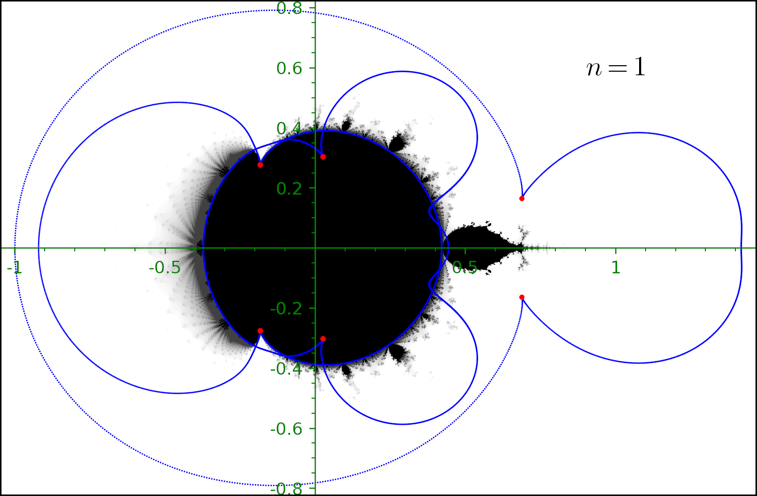
Figure S1: The convergence domain on the $\lambda$-plane for the first line of $A$ (the first eigenvector $z_{1}$) for the $3\times 3$ example. The Mandelbrot-like set (domain where orbits remain bounded) of the iterative scheme is shown in black and grey. The empirical convergence domain is shown in black. Its largest component corresponds to the stability of a steady state (the applicability domain of the iterative method). Small components correspond to stability of various periodic orbits. Various shades of grey show the values of $\lambda$ that lead to divergence to infinity (the darker the slower the divergence). In red are the values of $\lambda$ where the matrix is non-diagonalizable.

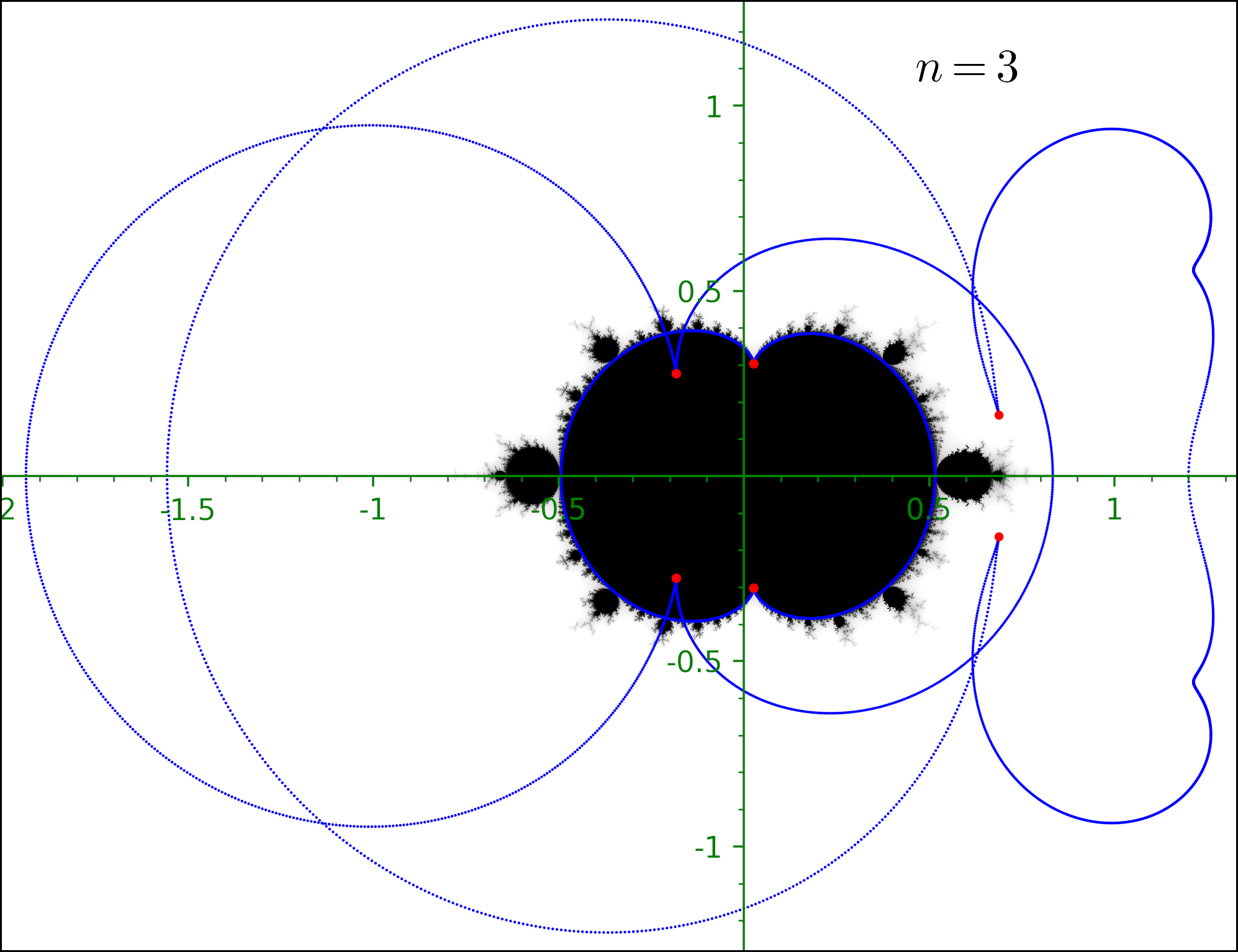
Figure S3: Same as Fig. S1 for the third eigenvector $z_{3}$ (the third line of $A$) .

As we can see, the dynamical systems for all three lines of $A$ ($n=1,2,3$) have different domains of convergence in the $\lambda$ plane. The corresponding curves are depicted on Fig. S1, Fig. S2, and Fig. S3, respectively.

There are differences also in curves for individuals lines with those for the $2\times 2$ case. Note that a curve $C$ does not contain enough information to find the convergence domain itself. The domains on Fig. S1–S3 were found empirically. Of course, they are bound by some parts of $C$ and include the point $\lambda=0$. The reason for some parts of $C$ not forming the boundary of the domain is that its different parts correspond to different eigenvectors. In other words, they belong to different branches of a multivalued eigenvector function of $\lambda$, the cusps being the branching points.

Consider as a particular example the case $n=2$. The curve $C$ intersects itself at $\lambda\approx-0.49$. Above the real axis about this point, one of the two intersecting branches of the curve form the convergence boundary. Below the real axis, the other one takes its place. This indicates that the two branches correspond to different multipliers of the same fixed point. When $\Im\lambda>0$, one of them crosses the unitary circle at the boundary of the convergence domain; when $\Im\lambda<0$, the other one does. At $\lambda\approx-0.49$, both of them cross the unitary circle simultaneously. This situation corresponds, thus, to a Neimark-Sacker bifurcation (the discrete time analog of the Andronov-Hopf bifurcation). Both branches are in fact parts of the same continuous curve that passes through the point $\lambda\approx 0.56$. Around this point, the curve poses no problem to the convergence of the dynamical system. The reason for this is that an excursion around cusps (branching points of eigenvectors) permutes some eigenvectors. As a consequence, the curve at $\lambda\approx-0.49$ corresponds to the loss of stability of the eigenvector that is a continuation of the unique stable eigenvector at $\lambda=0$ by the path $[0,-0.49]$. At the same time, the same curve at $\lambda\approx 0.56$ indicates a unitary by absolute value multiplier of an eigenvector that is not a continuation of the initial one by the path $[0,0.56]$.

Not all features of the curves depicted this $3\times 3$ case are generic either. The particular symmetry with respect to the complex conjugation of the curve and of its cusps is not generic for general complex matrices $D$ and $\Delta$, but it is a generic feature of matrices with real components. In this particular case, due to this symmetry, the only possible bifurcations for real values of $\lambda$ are the flip bifurcations (a multiplier equals to $-1$, typically followed by the cycle doubling cascade), the Neimark-Sacker bifurcation (two multipliers assume complex conjugate values $e^{\pm it}$ for some $t$), and, if the matrices are not symmetric, the fold bifurcation (a multiplier is equal to $1$). With symmetric real matrices, the fold bifurcation is not encountered because the cusps cannot be real but instead form complex conjugated pairs. These features are the consequence of the behavior of $\det(D+\lambda\Delta-xI)$ with respect to complex conjugation and from the fact that symmetric real matrices cannot have nontrivial Jordan forms.

Likewise, Hermitian matrices result in complex conjugate nonreal cusp pairs, but the curve itself is not necessarily symmetric. As a result, there are many more ways for a steady state to lose its stability, from which the fold bifurcation is, however, excluded. Generic bifurcations at $\lambda\in\mathbb{R}$ here consist in a multiplier getting a value $e^{it}$ for some $t\neq 0$. The situation for general complex matrices lacks any symmetry at all. Here steady states lose their stability by a multiplier crossing the unit circle with any value of $t$, and thus the fold bifurcation, although possible, is not generic. It is generic for one-parameter (in addition to $\lambda$) families of matrices.

As already noted, for the holomorphic dynamics of any $2\times 2$ case the unique critical point is guaranteed to be attracted by the unique attracting periodic orbit, if the latter exists. This, in turn, guarantees that for any $\Delta$ with zero diagonal the iteration of (2) starting from the identity matrix converges to the needed solution provided that $\lambda$ is in the convergence domain. This is not true anymore for $N>2$, starting already from the fact that there are no discrete critical points in larger dimensions. The problem of finding a good initial condition becomes non-trivial. As can be seen on Fig. S2, the particular $3\times 3$ case encounters this problem for the second line ($n=2$). The naive iteration with $A^{(0)}=I$ does not converge to the existing attracting fixed point of the dynamical system near some boundaries of its convergence domain. Our current understanding of this phenomenon is the crossing of the initial point by the attraction basin boundary (in the $z$-space). This boundary is generally fractal. Perhaps this explains the eroded appearance of the empirical convergence domain of the autonomous iteration.

To somewhat mitigate this complication, we applied a nonautonomous iteration scheme in the form, omitting details, $z^{(k+1)}=F_{2}(z^{(k)},\lambda(1-\alpha^{k}))$ with $z^{(0)}=(0,1,0)$, where $\alpha$ is some positive number $\alpha<1$, so that $\lim_{k\to\infty}\lambda(1-\alpha^{k})=\lambda$, and we explicitly indicated the dependence of $F_{2}(z,\lambda)$ on $\lambda$. The idea of this ad hoc approach is the continuation of the steady state in the extended $(z,\lambda)$-phase space from values of $\lambda$ that put $z^{(0)}$ inside the convergence domain of that steady state. Doing so, we managed to empirically recover the theoretical convergence domain (see Fig. S2).

Finally, we would like to point out an interesting generic occurrence of a unitary multiplier without the fold bifurcation. For $n=1$, this situation takes place at $\lambda\approx 0.45$, for $n=2$ at $\lambda\approx 0.56$, and for $n=3$ at $\lambda\approx 1.2$. All three points are on the real axis, as is expected from the symmetry considerations above. There is no cusp at these points and no fold bifurcations (no merging of eigenvectors), as it should be for symmetric real matrices. Instead, another multiplier of the same fixed point goes to infinity at the same value of $\lambda$ (the point becomes super-repelling). As a result, the theorem of the reduction to the central manifold is not applicable.

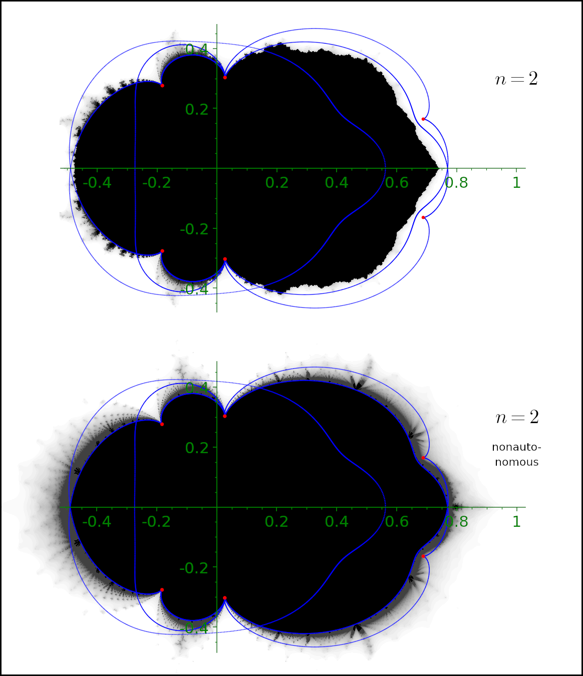
Figure S2: Same as Fig. S1 for the second eigenvector $z_{2}$ (the second line of $A$). Small components correspond to stability of various periodic orbits. Various shades of grey show the values of $\lambda$ that lead to divergence to infinity (the darker the slower the divergence).