DROCC: Deep Robust One-Class Classification

Abstract

Classical approaches for one-class problems such as one-class SVM and isolation forest require careful feature engineering when applied to structured domains like images. State-of-the-art methods aim to leverage deep learning to learn appropriate features via two main approaches. The first approach based on predicting transformations (Golan & El-Yaniv, 2018; Hendrycks et al., 2019a) while successful in some domains, crucially depends on an appropriate domain-specific set of transformations that are hard to obtain in general. The second approach of minimizing a classical one-class loss on the learned final layer representations, e.g., DeepSVDD (Ruff et al., 2018) suffers from the fundamental drawback of representation collapse. In this work, we propose Deep Robust One Class Classification (DROCC) that is both applicable to most standard domains without requiring any side-information and robust to representation collapse. DROCC is based on the assumption that the points from the class of interest lie on a well-sampled, locally linear low dimensional manifold. Empirical evaluation demonstrates that DROCC is highly effective in two different one-class problem settings and on a range of real-world datasets across different domains: tabular data, images (CIFAR and ImageNet), audio, and time-series, offering up to 20% increase in accuracy over the state-of-the-art in anomaly detection. Code is available at https://github.com/microsoft/EdgeML.

1 Introduction

In this work, we study “one-class” classification where the goal is to obtain accurate discriminators for a special class. Anomaly detection is one of the most well-known problems in this setting where we want to identify outliers, i.e. points that do not belong to the typical data (special class). Another related setting under this framework is classification from limited negative training instances where we require low false positive rate at test time even over close negatives. This is common in AI systems such as wake-word detection where the wake-words form the positive or special class, and for safe operation in the real world, the system should not fire on inputs that are close but not identical to the wake-words, no matter how the training data was sampled.

Anomaly detection is a well-studied problem with a large body of research (Aggarwal, 2016; Chandola et al., 2009). Classical approaches for anomaly detection are based on modeling the typical data using simple functions over the inputs (Schölkopf et al., 1999; Liu et al., 2008; Lakhina et al., 2004), such as constructing a minimum-enclosing ball around the typical data points (Tax & Duin, 2004). While these techniques are well-suited when the input is featurized appropriately, they struggle on complex domains like vision and speech, where hand-designing features is difficult.

In contrast, deep learning based anomaly detection methods attempt to automatically learn features, e.g., using CNNs in vision (Ruff et al., 2018). However, current approaches to do so have fundamental limitations. One family of approaches is based on extending the classical data modeling techniques over the learned representations. However, learning these representations jointly with the data modeling layer might lead to degenerate solutions where all the points are mapped to a single point (like origin), and the data modeling layer can now perfectly “fit” the typical data. Recent works like (Ruff et al., 2018) have proposed some heuristics to mitigate this like setting the bias to zero, but such heuristics are often insufficient in practice (Table 1). The second line of work (Golan & El-Yaniv, 2018; Bergman & Hoshen, 2020; Hendrycks et al., 2019b) is based on learning the salient geometric structure of the typical data (e.g., orientation of the object) by applying specific transformations (e.g., rotations and flips) to the input data and training the discriminator to predict applied transformation. If the discriminator fails to predict the transform accurately, the input does not have the same orientation as typical data and is considered anomalous. In order to be successful, these works critically rely on side-information in the form of appropriate structure/transformations, which is difficult to define in general, especially for domains like time-series, speech, etc. Even for images, if the normal data has been captured from multiple orientations, it is difficult to find appropriate transformations. The last set of deep anomaly detection techniques use generative models such as autoencoders or generative-adversarial networks (GANs) (Schlegl et al., 2017a) to learn to generate the entire typical data distribution which can be challenging and inaccurate in practice (Table 1).

In this paper, we propose a novel Deep Robust One-Class Classifiation (DROCC) method for anomaly detection that attempts to address the drawbacks of previous methods detailed above. DROCC is robust to representation collapse by involving a discriminative component that is general and is empirically accurate on most standard domains like tabular, time-series and vision without requiring any additional side-information. DROCC is motivated by the key observation that generally, the typical data lies on a low-dimensional manifold, which is well-sampled in the training data. This is believed to be true even in complex domains such as vision, speech, and natural language (Pless & Souvenir, 2009). As manifolds resemble Euclidean space locally, our discriminative component is based on classifying a point as anomalous if it is outside the union of small $\ell_{2}$ balls around the training typical points (See Figure 1a for an illustration). Importantly, the above definition allows us to synthetically generate anomalous points, and we adaptively generate the most effective anomalous points while training via a gradient ascent phase reminiscent of adversarial training. In other words, DROCC has a gradient ascent phase to adaptively add anomalous points to our training set and a gradient descent phase to minimize the classification loss by learning a representation and a classifier on top of the representations to separate typical points from the generated anomalous points. In this way, DROCC automatically learns an appropriate representation (like DeepSVDD) but is robust to a representation collapse as mapping all points to the same value would lead to poor discrimination between normal points and the generated anomalous points.

Next, we study a critical problem similar in flavor to anomaly detection and outlier exposure (Hendrycks et al., 2019a), which we refer to as One-class Classification with Limited Negatives (${\rm OCLN}$). The goal of ${\rm OCLN}$ is to design a one-class classifier for a positive class with only limited negative instances—the space of negatives is huge and is not well-sampled by the training points. The ${\rm OCLN}$ classifier should have low FPR against arbitrary distribution of negatives (or uninteresting class) while still ensuring accurate prediction accuracy for positives. For example, consider audio wake-word detection, where the goal is to identify a certain word, say Marvin in a given speech stream. For training, we collect negative instances where Marvin has not been uttered. Standard classification methods tend to identify simple patterns for classification, often relying only on some substring of Marvin say Mar. While such a classifier has good accuracy on the training set, in practice, it can have a high FPR as the classifier will mis-fire on utterances like Marvelous or Martha. This exact setting has been relatively less well-studied, and there is no benchmark to evaluate methods. Existing work suggests to simply expand the training data to include false positives found after the model is deployed, which is expensive and oftentimes infeasible or unsafe in real applications.

In contrast, we propose DROCC–LF, an outlier-exposure style extension of DROCC. Intuitively, DROCC–LF combines DROCC’s anomaly detection loss (that is over only the positive data points) with standard classification loss over the negative data. But, in addition, DROCC–LF exploits the negative examples to learn a Mahalanobis distance to compare points over the manifold instead of using the standard Euclidean distance, which can be inaccurate for high-dimensional data with relatively fewer samples.

We apply DROCC to standard benchmarks from multiple domains such as vision, audio, time-series, tabular data, and empirically observe that DROCC is indeed successful at modeling the positive (typical) class across all the above mentioned domains and can significantly outperform baselines. For example, when applied to the anomaly detection task on the benchmark CIFAR-10 dataset, our method can be up to 20% more accurate than the baselines like DeepSVDD (Ruff et al., 2018), Autoencoder (Sakurada & Yairi, 2014), and GAN based methods (Nguyen et al., 2019). Similarly, for tabular data benchmarks like Arrhythmia, DROCC can be $\geq 18$% more accurate than state-of-the-art methods (Bergman & Hoshen, 2020; Zong et al., 2018). Finally, for ${\rm OCLN}$ problem, our method can be upto 10% more accurate than standard baselines.

In summary, the paper makes the following contributions:

• We propose DROCC method that is based on a low-dimensional manifold assumption on the positive class using which it synthetically and adaptively generates negative instances to provide a general and robust approach to anomaly detection.

• We extend DROCC to a one-class classification problem where low FPR on arbitrary negatives is crucial. We also provide an experimental setup to evaluate different methods for this important but relatively less studied problem.

• Finally, we experiment with DROCC on a wide range of datasets across different domains–image, audio, time-series data and demonstrate the effectiveness of our method compared to baselines.

2 Related Work

Anomaly Detection (AD) has been extensively studied owing to its wide applicabilty (Chandola et al., 2009; Goldstein & Uchida, 2016; Aggarwal, 2016). Classical techniques use simple functions like modeling normal points via low-dimensional subspace or a tree-structured partition of the input space to detect anomalies (Schölkopf et al., 1999; Tax & Duin, 2004; Liu et al., 2008; Lakhina et al., 2004; Gu et al., 2019). In contrast, deep AD methods attempt to learn appropriate features, while also learning how to model the typical data points using these features. They broadly fall into three categories discussed below.

AD via generative modeling. Deep Autoencoders as well as GAN based methods have been studied extensively (Malhotra et al., 2016; Sakurada & Yairi, 2014; Nguyen et al., 2019; Li et al., 2018; Schlegl et al., 2017b). However, these methods solve a harder problem as they require reconstructing the entire input from its low-dimensional representation during the decoding step. In contrast, DROCC directly addresses the goal of only identifying if a given point lies somewhere on the manifold, and hence tends to be more accurate in practice (see Table 1, 2, 3).

Deep Once Class SVM: Deep SVDD (Ruff et al., 2018) introduced the first deep one-class classification objective for anomaly detection, but suffers from representation collapse issue (see Section 1). In contrast, DROCC is robust to such collapse since the training objective requires representations to allow for accurate discrimination between typical data points and their perturbations that are off the manifold of the typical data points.

Transformations based methods: Recently, (Golan & El-Yaniv, 2018; Hendrycks et al., 2019b) proposed another approach to AD based on self-supervision. The training procedure involves applying different transformations to the typical points and training a classifier to identify the transform applied. The key assumption is that a point is normal iff the transformations applied to the point can be correctly identified, i.e., normal points conform to a specific structure captured by the transformations. (Golan & El-Yaniv, 2018; Hendrycks et al., 2019b) applied the method to vision datasets and proposed using rotations, flips etc as the transformations. (Bergman & Hoshen, 2020) generalized the method to tabular data by using handcrafted affine transforms. Naturally, the transformations required by these methods are heavily domain dependent and are hard to design for domains like time-series. Furthermore, even for vision tasks, the suitability of a transformation varies based on the structure of the typical points. For example, as discussed in (Golan & El-Yaniv, 2018), horizontal flips perform well when the typical points are from class ’3’ (AUROC 0.957) of MNIST but perform poorly when typical points are from class ’8’ (AUROC 0.646). In contrast, the low-dimensional manifold assumption that motivates DROCC is generic and seems to hold across several domains like images, speech, etc. For example, DROCC obtains AUROC of $\sim$ 0.97 on both typical class ’8’ and typical class ’3’ in MNIST. (See Section 5 for more comparison with self-supervision based techniques)

Side-information based AD: Recently, several AD methods to explicitly incorporate side-information have been proposed. (Hendrycks et al., 2019a) leverages access to a few out-of-distribution samples, (Ruff et al., 2020) explores the semisupervised setting where a small set of labeled anomalous examples are available. We view these approaches as complementary to DROCC which does not assume any side-information. Finally, ${\rm OCLN}$ problem is generally modeled as a binary classification probelm, but outlier exposure (OE) style formulation (Hendrycks et al., 2019b) can be used to combine it with anomaly detection methods. Our method DROCC–LF builds upon OE approach but exploits the ”outliers” in a more integrated manner.

3 Anomaly Detection

Let $\mathcal{S}\subseteq\mathbb{R}^{d}$ denote the set of typical, i.e., non-anomalous data points. A point $x\in\mathbb{R}^{d}$ is anomalous or atypical if $x\not\in\mathcal{S}$. Suppose we are given $n$ samples $D=[x_{i}]_{i=1}^{n}\in\mathbb{R}^{d}$ as training data, where $D_{S}=\{x_{i}\mid x_{i}\in\mathcal{S}\}$ is the set of typical points sampled in the training data and $|D_{S}|\geq(1-\nu)|S|$ i.e. $\nu\ll 1$ fraction of points in $D$ are anomalies. Then, the goal in unsupervised anomaly detection (AD) is to learn a function $f_{\theta}:\mathbb{R}^{d}\mapsto\{-1,1\}$ such $f_{\theta}(x)=1$ when $x\in\mathcal{S}$ and $f_{\theta}(x)=-1$ when $x\not\in\mathcal{S}$. The anomaly detector is parameterized by some parameters $\theta$.

Algorithm 1 Training neural networks via DROCC

Input: Training data $D=[x_{1},x_{2},\ldots x_{n}]$.

Parameters: Radius $r$, $\lambda\geq 0$, $\mu\geq 0$, step-size $\eta$, number of gradient steps $m$, number of initial training steps $n_{0}$.

Initial steps: For $B=1,\ldots n_{0}$

$X_{B}$: Batch of training inputs

$\theta=\theta-\text{Gradient-Step}\Big{(}\sum\limits_{x\in X_{B}}\ell(f_{\theta}(x),1)\Big{)}$

DROCC steps: For $B=n_{0},\ldots n_{0}+N$

$X_{B}$: Batch of training inputs

$\forall x\in X_{B}:h\sim\mathcal{N}(0,I_{d})$

Adversarial search: For $i=1,\ldots m$

1. $\ell(h)=\ell(f_{\theta}(x+h),-1)$

2. $h=h+\eta\frac{\nabla_{h}\ell(h)}{\|\nabla_{h}\ell(h)\|}$

3. $h=\frac{\alpha}{\|h\|}\cdot h$ where $\alpha=r\cdot\mathds{1}[\|h\|\leq r]+\|h\|\cdot\mathds{1}[r\leq\hskip 60.0pt\|h\|\leq\gamma\cdot r]+\gamma\cdot r\cdot\mathds{1}[\|h\|\geq\gamma\cdot r]$

$\ell^{itr}=\lambda\|\theta\|^{2}+\sum\limits_{x\in X_{B}}\ell(f_{\theta}(x),1)+\mu\ell(f_{\theta}(x+h),-1)$

$\theta=\theta-\text{Gradient-Step}(\ell^{itr})$

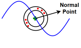
(a)

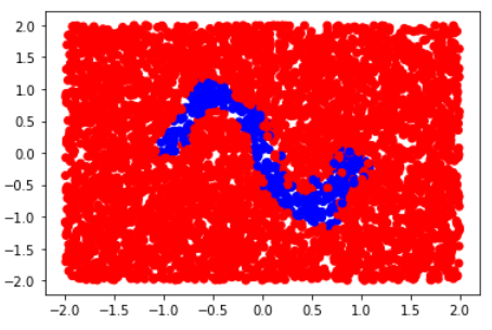
(b)

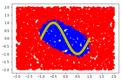
(c)

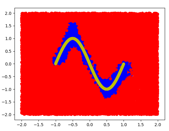
(d)

Figure 1: (a) A normal data manifold with red dots representing generated anomalous points in $N_{i}(r)$. (b) Decision boundary learned by DROCC when applied to the data from (a). Blue represents points classified as normal and red points are classified as abnormal. (c), (d): first two dimensions of the decision boundary of DROCC and DROCC–LF, when applied to noisy data (Section 5.2). DROCC–LF is nearly optimal while DROCC’s decision boundary is inaccurate. Yellow color sine wave depicts the train data.

Deep Robust One Class Classification: We now present our approach to unsupervised anomaly detection that we call Deep Robust One Class Classification (DROCC). Our approach is based on the following hypothesis: The set of typical points $\mathcal{S}$ lies on a low dimensional locally linear manifold that is well-sampled. In other words, outside a small radius around a training (typical) point, most points are anomalous. Furthermore, as manifolds are locally Euclidean, we can use the standard $\ell_{2}$ distance function to compare the points in a small neighborhood. Figure 1a shows a $1$-d manifold of the typical points and intuitively, why in a small neighborhood of the training points we can use $\ell_{2}$ distances. We label the typical points as positive and anomalous points as negative.

Formally, for a DNN architecture $f_{\theta}:\mathbb{R}^{d}\rightarrow\mathbb{R}$ parameterized by $\theta$, and a small radius $r>0$, DROCC estimates parameter $\theta^{dr}$ as : $\min_{\theta}\ell^{dr}(\theta)$, where,

$$\ell^{\text{dr}}(\theta)=\lambda\|\theta\|^{2}+\sum\limits_{i=1}^{n}[\ell(f_{\theta}(x_{i}),1)+\mu\max\limits_{\stackrel{{\scriptstyle\tilde{x}_{i}\in}}{{N_{i}(r)}}}\ell(f_{\theta}(\tilde{x}_{i}),-1)],\$$

$$N_{i}(r)\stackrel{{\scriptstyle\rm def}}{{=}}\Big{\{}\|\tilde{x}_{i}-x_{i}\|_{2}\leq\gamma\cdot r;\ \ r\leq\|\tilde{x}_{i}-x_{j}\|,\$$

$$\qquad\qquad~{}\forall j=1,2,\ldots n\Big{\}},$$ (1)

and $\lambda>0$, $\mu>0$ are regularization parameters. $N_{i}(r)$ captures points off the manifold, i.e., are at least at $r$ distance from all training points. We use an upper bound $\gamma\cdot r$ for regularizing the optimization problem where $\gamma\geq 1$. $\ell:\mathbb{R}\times\mathbb{R}\rightarrow\mathbb{R}$ is some classification loss function, and goal is to classify the given normal points $x_{i}$’s as positives while the generated anomalous examples $\tilde{x}_{i}$ as negatives.

The above given formulation is a saddle point problem and is similar to adversarial training where the network is trained to be robust to worst-case $\ell_{p}$ ball perturbations around the inputs (See, for example (Madry et al., 2018)). In DROCC, we replace the $\ell_{p}$ ball with $N_{i}(r)$, and adopt the standard projected gradient descent-ascent technique to solve the saddle point problem.

Gradient-ascent to generate negatives.

A key step in the gradient descent-ascent algorithm is that of projection onto the $N_{i}(r)$ set. That is, given $z\in\mathbb{R}^{d}$, the goal is to find $\tilde{x}_{i}=\arg\min_{u}\|u-z\|^{2}\ s.t.\ u\in N_{i}(r)$. Now, $N_{i}$ contains points that are less than $\gamma\cdot r$ distance away from $x_{i}$ and at least $r$ away from all $x_{j}$’s. The second constraint involves all the training points and is computationally challenging. So, for computational ease, we redefine $N_{i}(r)\stackrel{{\scriptstyle\rm def}}{{=}}\Big{\{}r\leq\|\tilde{x}_{i}-x_{i}\|_{2}\leq\gamma\cdot r\Big{\}}$. In practice, since the positive points in $\mathcal{S}$ lie on a low dimensional manifold, we empirically find that the adversarial search over this set does not yield a point that is in $\mathcal{S}$. Further, we use a lower weight on the classification loss of the generated negatives so as to guard against possible non-anomalous points in $N_{i}(r)$. Finally, projection onto this set is given by $\tilde{x}_{i}=x_{i}+\alpha\cdot(z-x_{i})$ where $\beta=\|z-x_{i}\|$, and $\alpha=\gamma r/\beta$ if $\beta\geq\gamma r$ (point is too far), $\alpha=r/\beta$ if $\beta\leq r$ and $\alpha=1$ otherwise.

Algorithm 1 summarizes our DROCC method. The three steps in the adversarial search are performed in parallel for each $x\in B$ the batch; for simplicity, we present the procedure for a single example $x$. In step one, we compute the loss of the network with respect to a negative label (anomalous point) where we express $\tilde{x}$ as $x+h$. In step two, we maximize this loss in order to find the most “adversarial” point via normalized steepest ascent. Finally, we project $\tilde{x}$ onto $N_{i}(r)$. In order to update the parameters of the network, we could use any gradient based update rule such as SGD or other adaptive methods like Adagrad or Adam. We typically set $\gamma=2$. Parameters $\lambda,\mu,\eta$ are selected via cross-validation. Note that our method allows arbitrary DNN architecture $f_{\theta}$ to represent and classify data points $x_{i}$. Finally, we set $\ell$ to be the standard cross-entropy loss.

4 One-class Classification with Limited Negatives (${\rm OCLN}$)

In this section, we extend DROCC to address the ${\rm OCLN}$ problem. Let $D=[(x_{1},y_{1}),\dots,(x_{n},y_{n})]$ be a given set of points where $x_{i}\in\mathbb{R}^{d}$ and $y_{i}\in\{1,-1\}$. Furthermore, let the mass of positive points’ distribution covered by the training data is significantly higher than that of negative points’ distribution. For example, if data points are sampled from a discrete distribution, with $P_{+}$ being the marginal distribution of the positive points and $P_{-}$ be the margin distribution of the negative points. Then, the assumption is: $\frac{1}{n_{-}}\sum_{i,y_{i}=-1}P_{-}(x_{i})\ll\frac{1}{n_{+}}\sum_{i,y_{i}=1}P_{+}(x_{i})$ where $n_{+}$, $n_{-}$ are the number of positive and negative training points.

The goal of ${\rm OCLN}$ is similar to anomaly detection (AD), that is, to identify arbitrary outliers–negative class in this case–correctly despite limited access to negatives’ data distribution. So it is an AD problem with side-information in the form of limited negatives. Intuitively, ${\rm OCLN}$ problems arise in domains where data for special positive class (or set of classes) can be collected thoroughly, but the “negative” class is a catch-all class that cannot be sampled thoroughly due to its sheer size. Several real-world problems can be naturally modeled by ${\rm OCLN}$. For example, consider wake word detection problems where the goal is to identify a special audio command to wake up the system. Here, the data for a special wake word can be collected exhaustively, but the negative class, which is “everything else” cannot be sampled properly.

Naturally, we can directly apply standard AD methods (e.g., DROCC) or binary classification methods to the problem. However, AD methods ignore the side-information, while the classification methods’ might generalize only to the training distribution of negatives and hence might have high False Positive Rate (FPR) in the presence of negatives far from the train distribution. Instead, we propose method DROCC–OE that uses an approach similar to outlier exposure (Hendrycks et al., 2019a), where the optimization function is given by a summation of the anomaly detection loss and standard cross entropy loss over negatives. The intuition behind DROCC–OE is that the positive data satisfies the manifold hypothesis of the previous section, and hence points off the manifold should be classified as negatives. But the process can be bootstrapped by explicit negatives from the training data.

Next, we propose DROCC–LF which integrates information from the negatives in a deeper manner than DROCC–OE. In particular, we use negatives to learn input coordinates or features which are noisy and should be ignored. As DROCC uses Euclidean distance to compare points locally, it might struggle due to the noisy coordinates, which DROCC–LF will be able to ignore. Formally, DROCC–LF estimates parameter $\theta^{\text{lf}}$ as: $\min_{\theta}\ell^{lf}(\theta)$ where,

$$\ell^{lf}(\theta)=\lambda\|\theta\|^{2}+\sum\limits_{i=1}^{n}[\ell(f_{\theta}(x_{i}),y_{i})+\mu\max\limits_{\stackrel{{\scriptstyle\tilde{x}_{i}\in}}{{N_{i}(r)}}}\ell(f_{\theta}(\tilde{x}_{i}),-1)],\$$

$$\qquad\qquad N_{i}(r):=\{\tilde{x}_{i},\ s.t.,\ r\leq\|\tilde{x}_{i}-x_{i}\|_{\Sigma}\leq\gamma\cdot r\},$$ (2)

and $\lambda>0$, $\mu>0$ are regularization parameters. Instead of Euclidean distance, we use Mahalanobis distance function $\|\tilde{x}-x\|_{\Sigma}^{2}=\sum_{j}\sigma_{j}(\tilde{x}^{j}-x^{j})^{2}$ where $x^{j},\tilde{x}^{j}$ are the $j$-th coordinate of $x$ and $\tilde{x}$, respectively. $\sigma_{j}:=\left|\frac{\partial f_{\theta(x)}}{\partial x_{j}}\right|$, i.e., $\sigma_{j}$ measures the ”influence” of $j$-th coordinate on the output, and is updated every epoch during training.

Similar to (1), we can use the standard projected gradient descent-ascent algorithm to optimize the above given saddle point problem. Here again, projection onto $N_{i}(r)$ is the key step. That is, the goal is to find: $\tilde{x}_{i}=\arg\min_{x}\|x-z\|^{2}\ s.t.\ x\in N_{i}(r)$. Unlike, Section 3 and Algorithm 1, the above projection is unlikely to be available in closed form and requires more careful arguments.

Proposition 1.

Consider the problem: $\min_{\tilde{x}}\|\tilde{x}-z\|^{2},\ s.t.,\ r^{2}\leq\|\tilde{x}-x\|_{\Sigma}^{2}\leq\gamma^{2}r^{2}$ and let $\delta=z-x$. If $r\leq\|\delta\|_{\Sigma}\leq\gamma r$, then $\tilde{x}=z$. Otherwise, the optimal solution is : $\tilde{x}=x+(I+\tau\Sigma)^{-1}\delta,$ where :
1) If $\|\delta\|_{\Sigma}\leq r$,
$\tau:=\arg\min_{\tau\leq 0}\sum_{j}\frac{\delta_{j}^{2}\tau^{2}\sigma_{j}^{2}}{(1+\tau\sigma_{j})^{2}},\ s.t.,\ \sum_{j}\frac{\delta_{j}^{2}\sigma_{j}}{(1+\tau\sigma_{j})^{2}}\geq r^{2},$
2) If $\|\delta\|_{\Sigma}\geq\gamma\cdot r$,
$\tau^{-1}:=\arg\min_{\nu\geq 0}\sum_{j}\frac{\delta_{j}^{2}\sigma_{j}^{2}}{(\nu+\sigma_{j})^{2}},\ s.t.,\ \sum_{j}\frac{\delta_{j}^{2}\sigma_{j}\nu^{2}}{(\nu+\sigma_{j})^{2}}\leq\gamma^{2}r^{2}$ .

See Appendix A for a detailed proof. The above proposition reduces the projection problem to a non-convex but one-dimensional optimization problem. We solve this problem via standard grid search over: $\tau=[-\frac{1}{\max_{j}\sigma_{j}},0]$ or $\nu=[0,\frac{\alpha}{1-\alpha}\max_{j}\sigma_{j}]$ where $\alpha=\gamma\cdot r/\|\delta\|_{\Sigma}$. The algorithm is now almost same as Algorithm 1 but uses the above mentioned projection algorithm; see Appendix A for a pseudo-code of our DROCC–LF method.

4.1 ${\rm OCLN}$ Evaluation Setup

Due to lack of benchmarks, it is difficult to evaluate a solution for ${\rm OCLN}$. So, we provide a novel experimental setup for a wake-word detection and a digit classification problem, showing that DROCC–LF indeed significantly outperforms standard anomaly detection, binary classification, and DROCC–OE on practically relevant metrics (Section 5.2).

In particular, our setup is inspired by standard settings encountered by real-world detection problems. For example, consider the wakeword detection problem, where the goal is to detect a wakeword like say ”Marvin” in a continuous stream of data. In this setting, we are provided a few positive examples for Marvin and a few generic negative examples from everyday speech. But, in our experiment setup, we generate close or difficult negatives by generating examples like Arvin, Marvelous etc. Now, in most real-world deployments, a critical requirement is low False Positive Rates, even on such difficult negatives. So, we study various methods with FPR bounded by say 3% or 5% on negative data that comprises of generic negatives as well as difficult close negatives. Now, under FPR constraint, we evaluate various methods by their recall rate, i.e., based on how many true positives the method is able to identify. We propose a similar setup for a digit classification problem as well; see Section 5.2 for more details.

5 Empirical Evaluation

In this section, we present empirical evaluation of DROCC on two one-class classification problems: Anomaly Detection and One-Class Classification with Limited Negatives (${\rm OCLN}$). We discuss the experimental setup, datasets, baselines, and the implementation details. Through experimental results on a wide range of synthetic and real-world datasets, we present strong empirical evidence for the effectiveness of our approach for one-class classification problems.

Table 1: Average AUC (with standard deviation) for one-vs-all anomaly detection on CIFAR-10. DROCC outperforms baselines on most classes, with gains as high at 20%, and notably, nearest neighbours beats all the baselines on 2 classes.

CIFAR Class	OC-SVM	IF	DCAE	AnoGAN	ConAD 16	Soft-Bound Deep SVDD	One-Class Deep SVDD	Nearest Neighbour	DROCC (Ours)
Airplane	61.6$\pm$0.9	60.1$\pm$0.7	59_1$\pm$5_1	67.1$\pm$2.5	77.2	61.7$\pm$4.2	61.7$\pm$4.1	69.02	81.66 $\pm$ 0.22
Automobile	63.8$\pm$0.6	50.8$\pm$0.6	57.4$\pm$2.9	54.7$\pm$3.4	63.1	64.8$\pm$1.4	65.9$\pm$2.1	44.2	76.738 $\pm$ 0.99
Bird	50.0$\pm$0.5	49.2$\pm$0.4	48.9$\pm$2.4	52.9$\pm$3.0	63.1	49.5$\pm$1.4	50.8$\pm$0.8	68.27	66.664 $\pm$ 0.96
Cat	55.9$\pm$1.3	55.1$\pm$0.4	58.4$\pm$1.2	54.5$\pm$1.9	61.5	56.0$\pm$1.1	59.1$\pm$1.4	51.32	67.132 $\pm$ 1.51
Deer	66.0$\pm$0.7	49.8$\pm$0.4	54.0$\pm$1.3	65.1$\pm$3.2	63.3	59.1$\pm$1.1	60.9$\pm$1.1	76.71	73.624 $\pm$ 2.00
Dog	62.4$\pm$0.8	58.5$\pm$0.4	62.2$\pm$1.8	60.3$\pm$2.6	58.8	62.1$\pm$2.4	65.7$\pm$2.5	49.97	74.434 $\pm$ 1.95
Frog	74.7$\pm$0.3	42.9$\pm$0.6	51.2$\pm$5.2	58.5$\pm$1.4	69.1	67.8$\pm$2.4	67.7$\pm$2.6	72.44	74.426 $\pm$ 0.92
Horse	62.6$\pm$0.6	55.1$\pm$0.7	58.6$\pm$2.9	62.5$\pm$0.8	64.0	65.2$\pm$1.0	67.3$\pm$0.9	51.13	71.39 $\pm$ 0.22
Ship	74.9$\pm$0.4	74.2$\pm$0.6	76.8$\pm$1.4	75.8$\pm$4.1	75.5	75.611.7	75.9$\pm$1.2	69.09	80.016 $\pm$ 1.69
Truck	75.9$\pm$0.3	58.9$\pm$0.7	67.3$\pm$3.0	66.5$\pm$2.8	63.7	71.0$\pm$1.1	73.1$\pm$1.2	43.33	76.21 $\pm$ 0.67

5.1 Anomaly Detection

Datasets: In all the experiments with multi-class datasets, we follow the standard one-vs-all setting for anomaly detection: fixing each class once as nominal and treating rest as anomaly. The model is trained only on the nominal class but the test data is sampled from all the classes. For timeseries datasets, N represents the number of time-steps/frames and d represents the input feature length.

We perform experiments on the following datasets:

• 2-D sine-wave: 1000 points sampled uniformly from a 2-dimensional sine wave (see Figure 1a).

• Abalone (Dua & Graff, 2017): Physical measurements of abalone are provided and the task is to predict the age. Classes 3 and 21 are anomalies and classes 8, 9, and 10 are normal (Das et al., 2018).

• Arrthythmia (Rayana, 2016): Features derived from ECG and the task is to identify arrhythmic samples. Dimensionality is 279 but five categorical attributes are discarded. Dataset preparation is similar to Zong et al. (2018).

• Thyroid (Rayana, 2016): Determine whether a patient referred to the clinic is hypothyroid based on patient’s medical data. Only 6 continuous attributes are considered. Dataset preparation is same as Zong et al. (2018).

• Epileptic Seizure Recognition (Andrzejak et al., 2001): EEG based time-series dataset from multiple patients. Task is to identify if EEG is abnormal (N = 178, d = 1).

• Audio Commands (Warden, 2018): A multiclass data with 35 classes of audio keywords. Data is featurized using MFCC features with 32 filter banks over 25ms length windows with stride of 10ms ($N=98$, $d=32$). Dataset preparation is same as Kusupati et al. (2018).

• CIFAR-10 (Krizhevsky, 2009): Widely used benchmark for anomaly detection, 10 classes with $32\times 32$ images.

• ImageNet-10: a subset of 10 randomly chosen classes from the ImageNet dataset (Deng et al., 2009) which contains $224\times 224$ color images.

The datasets which we use are all publicly available. We use the train-test splits when already available with a 80-20 split for train and validation set. In all other cases, we use random 60-20-20 split for train, validation, and test.

DROCC Implementation: The main hyper-parameter of our algorithm is the radius $r$ which defines the set $N_{i}(r)$. We observe that tweaking radius value around $\sqrt{d}/2$ (where d is the dimension of the input data ) works the best, as due to zero-mean, unit-variance normalized features, the average distance between random points is $\approx\sqrt{d}$. We fix $\gamma$ as 2 in our experiments unless specified otherwise. Parameter $\mu$ (1) is chosen from {0.5 , 1.0}. We use a standard step size from {0.1, 0.01} for gradient ascent and from $\{10^{-2},10^{-4}\}$ for gradient descent; we also tune the optimizer $\in$ {Adam, SGD}. See Appendix D for a detailed ablation study. The implementation is available as part of the EdgeML package (Dennis et al., ). The experiments were run on an Intel Xeon CPU with 12 cores clocked at 2.60 GHz and with NVIDIA Tesla P40 GPU, CUDA 10.2, and cuDNN 7.6.

5.1.1 Results

Synthetic Data: We present results on a simple 2-D sine wave dataset to visualize the kind of classifiers learnt by DROCC. Here, the positive data lies on a 1-D manifold given in Figure 1a. We observe from Figure 1b that DROCC is able to capture the manifold accurately; whereas the classical methods OC-SVM and DeepSVDD (shown in Appendix B) perform poorly as they both try to learn a minimum enclosing ball for the whole set of positive data points.

Table 2: F1-Score (with standard deviation) for one-vs-all anomaly detection on Thyroid, Arrhythmia, and Abalone datasets. DROCC outperforms the baselines on all the three datasets.

	F1-Score
Method	Thyroid	Arrhythmia	Abalone
OC-SVM (Schölkopf et al., 1999)	0.39 $\pm$ 0.01	0.46 $\pm$ 0.00	0.48 $\pm$ 0.00
DCN(Caron et al., 2018)	0.33 $\pm$ 0.03	0.38 $\pm$ 0.03	0.40 $\pm$ 0.01
E2E-AE (Zong et al., 2018)	0.13 $\pm$ 0.04	0.45 $\pm$ 0.03	0.33 $\pm$ 0.03
LOF (Breunig et al., 2000)	0.54 $\pm$ 0.01	0.51 $\pm$ 0.01	0.33 $\pm$ 0.01
DAGMM (Zong et al., 2018)	0.49 $\pm$ 0.04	0.49 $\pm$ 0.03	0.20 $\pm$ 0.03
DeepSVDD (Ruff et al., 2018)	0.73 $\pm$ 0.00	0.54 $\pm$ 0.01	0.62 $\pm$ 0.01
GOAD (Bergman & Hoshen, 2020)	0.72 $\pm$ 0.01	0.51 $\pm$ 0.02	0.61 $\pm$ 0.02
DROCC (Ours)	0.78 $\pm$ 0.03	0.69 $\pm$ 0.02	0.68 $\pm$ 0.02

Tabular Data: Table 2 compares DROCC against various classical algorithms: OC-SVM, LOF(Breunig et al., 2000) as well as deep baselines: DCN(Caron et al., 2018), Autoencoder (Zong et al., 2018), DAGMM(Zong et al., 2018), DeepSVDD and GOAD(Bergman & Hoshen, 2020) on the widely used benchmark datasets, Arrhythmia, Thyroid and Abalone. In line with prior work, we use the F1- Score for comparing the methods (Bergman & Hoshen, 2020; Zong et al., 2018). A fully-connected network with a single hidden layer is used as the base network for all the deep baselines. We observe significant gains across all the three datasets for DROCC, as high as 18% in Arrhythmia.

Table 3: AUC (with standard deviation) for one-vs-all anomaly detection on Epileptic Seizures and Audio Keyword “Marvin”. DROCC outperforms the baselines on both the datasets

Method	AUC
	Epileptic Seizure	Audio Keywords
kNN	91.75	65.81
AE (Sakurada & Yairi, 2014)	91.15 $\pm$ 1.7	51.49 $\pm$ 1.9
REBM (Zhai et al., 2016)	97.24 $\pm$ 2.1	63.73 $\pm$ 2.4
DeepSVDD (Ruff et al., 2018)	94.84 $\pm$ 1.7	68.38 $\pm$ 1.8
DROCC (Ours)	98.23 $\pm$ 0.7	70.21 $\pm$ 1.1

Time-Series Data: There is a lack of work on anomaly detection for time-series datasets. Hence we extensively evaluate our method DROCC against deep baselines like AutoEncoders (Sakurada & Yairi, 2014), REBM (Zhai et al., 2016) and DeepSVDD. For autoencoders, we use the architecture presented in Srivastava et al. (2015). A single layer LSTM is used for all the deep baselines. Motivated by recent analysis (Gu et al., 2019), we also include nearest neighbours as a baseline. Table 3 compares the performance of DROCC against these baselines on the univariate Epileptic Seizure dataset, and the Audio Commands dataset. DROCC outperforms the baselines on both the datasets.

Image Data: For experiments on image datasets, we fixed $\gamma$ as 1. Table 1 compares DROCC on CIFAR-10 against baseline numbers from OC-SVM (Schölkopf et al., 1999), IF (Liu et al., 2008), DCAE (Seeböck et al., 2016), AnoGAN (Schlegl et al., 2017b), DeepSVDD as reported by Ruff et al. (2018) and against ConvAD16 as reported by Nguyen et al. (2019). Again, we include nearest neighbours as one of the baselines. LeNet (LeCun et al., 1998) architecture was used for all the baselines and DROCC for this experiment. DROCC consistently achieves the best performance on most classes, with gains as high as 20% over DeepSVDD on some classes. An interesting observation is that for the classes Bird and Deer, Nearest Neighbour achieves competitive performance, beating all the other baselines.

As discussed in Section 2, (Golan & El-Yaniv, 2018; Hendrycks et al., 2019b) use domain specific transformations like flip and rotations to perform the AD task. The performance of these approaches is heavily dependent on the interaction between transformations and the dataset. They would suffer significantly in more realistic settings where the images of normal class itself have been captured from multiple orientations. For example, even in CIFAR, for airplane class, the accuracy is relatively low (DROCC is 7% more accurate) as the images have airplanes in multiple angles. In fact, we try to mimic a more realistic scenario by augmenting the CIFAR-10 data with flips and small rotations of angle $\pm 30^{\circ}$. Table 4 depicts the drop in performance of GEOM when augmentations are added in the CIFAR-10 dataset. For example, on the deer class of CIFAR-10 dataset, GEOM has an AUC of 87.8%, which falls to 65.8% when augmented CIFAR-10 is used whereas DROCC ’s performance remains the same ($\sim 72\%$).

Next, we benchmark the performance of DROCC on high resolution images that require the use of large modern neural architectures. Table 5 presents the results of our experiments on ImageNet. DROCC continues to achieve the best results amongst all the compared methods. Autoencoder fails drastically on this dataset, so we exclude comparisons. For DeepSVDD and DROCC, MobileNetv2 (Sandler et al., 2018b) architecture is used. We observe that for all classes, except golf ball, DROCC outperforms the baselines. For instance, on French-Horn vs. rest problem, DROCC is 23% more accurate than DeepSVDD.

Table 4: Comparing DROCC against GEOM (Golan & El-Yaniv, 2018) on CIFAR-10 data flipped and rotated by a small angle of $\pm 30$ degree

CIFAR-10 Class	GEOM (No Aug)	DROCC (No Aug)	GEOM (with Aug)	DROCC (with Aug)
Airplane	74.7 $\pm$ 0.4	81.6 $\pm$ 0.2	62.4 $\pm$ 1.7	77.2 $\pm$ 1.2
Automobile	95.7 $\pm$ 0.0	76.7 $\pm$ 1.0	71.8 $\pm$ 1.2	74.5 $\pm$ 1.8
Bird	78.1 $\pm$ 0.4	66.7 $\pm$ 1.0	50.6 $\pm$ 0.5	67.5 $\pm$ 1.0
Cat	72.4 $\pm$ 0.5	67.1 $\pm$ 1.5	52.5 $\pm$ 0.7	68.8 $\pm$ 2.3
Deer	87.8 $\pm$ 0.2	73.6 $\pm$ 2.0	65.7 $\pm$ 1.7	71.1 $\pm$ 2.9
Dog	87.8 $\pm$ 0.1	74.4 $\pm$ 1.9	69.6 $\pm$ 1.3	71.3 $\pm$ 0.4
Frog	83.4 $\pm$ 0.5	74.4 $\pm$ 0.9	68.3 $\pm$ 1.1	71.2 $\pm$ 1.6
Horse	95.5 $\pm$ 0.1	71.4 $\pm$ 0.2	84.8 $\pm$ 0.8	63.5 $\pm$ 3.5
Ship	93.3 $\pm$ 0.0	80.0 $\pm$ 1.7	79.6 $\pm$ 2.2	76.4 $\pm$ 3.5
Truck	91.3 $\pm$ 0.1	76.2 $\pm$ 0.7	85.7 $\pm$ 0.5	74.0 $\pm$ 1.0

Table 5: Average AUC (with standard deviation) for one-vs-all anomaly detection on ImageNet. DROCC consistently achieves the best performance for all but one class.

ImageNet Class	Nearest Neighbor	DeepSVDD	DROCC (Ours)
Tench	65.57	65.14 $\pm$ 1.03	70.19 $\pm$ 1.7
English Springer	56.37	66.45 $\pm$ 3.16	70.45 $\pm$ 4.99
Cassette Player	47.7	60.47 $\pm$ 5.35	71.17 $\pm$ 1
Chainsaw	45.22	59.43 $\pm$ 4.13	68.63 $\pm$ 1.86
Church	61.35	56.31 $\pm$ 4.23	67.46 $\pm$ 4.17
French Horn	50.52	53.06 $\pm$ 6.52	76.97 $\pm$ 1.67
Garbage Truck	54.2	62.15 $\pm$ 4.39	69.06 $\pm$ 2.34
Gas Pump	47.43	56.66 $\pm$ 1.49	69.94 $\pm$ 0.57
Golf Ball	70.36	72.23 $\pm$ 3.43	70.72 $\pm$ 3.83
Parachute	75.87	81.35 $\pm$ 3.73	93.5 $\pm$ 1.41

5.2 One-class Classification with Limited Negatives (${\rm OCLN}$)

Recall that the goal in ${\rm OCLN}$ is to learn a classifier that is accurate for both, the in-sample positive (or normal) class points and for the arbitrary out-of-distribution (OOD) negatives. Naturally, the key metric for this problem is False Positive Rate (FPR). In our experiments, we bound any method to have FPR to be smaller than a threshold, and under that constraint, we measure it’s recall value, i.e., the fraction of true positives that are correctly predicted.

We compare DROCC–LF against the following baselines: a) Standard binary classifier: that is, we ignore the challenge of OOD negatives and treat the problem as a standard classification task, b) DeepSAD (Ruff et al., 2020): a semi-supervised anomaly detection method but it is not explicitly designed to handle negatives that are very close to positives (OOD negatives) and c) DROCC–OE: Outlier exposure type extension where DROCC’s anomaly detection loss (based on using Euclidean distance as a local distance measure over the manifold) is combined with standard cross-entropy loss over the given limited negative data. Similar to the anomaly detection experiments, we use the same underlying network architecture across all the baselines.

5.2.1 Results

Synthetic Data: We sample $1024$ points in $\mathbb{R}^{10}$, where the first two coordinates are sampled from the 2D-sine wave, as in the previous section. Coordinates $3$ to $10$ are sampled from the spherical Gaussian distribution. Note that due to the 8 noisy dimensions, DROCC would be forced to set $r=\sqrt{d}$ where $d=10$, while the true low-dimensional manifold is restricted to only two dimensions. Consequently, it learns an inaccurate boundary as shown in Figure 1c and is similar to the boundary learned by OC-SVM and DeepSVDD; points that are predicted to be positive by DROCC are colored blue. In contrast, DROCC–LF is able to learn that only the first two coordinates are useful for the distinction between positives and negatives, and hence is able to learn a skewed distance function, leading to an accurate decision boundary (see Figure 1d).

MNIST 0 vs. 1 Classification: We consider an experimental setup on MNIST dataset, where the training data consists of Digit $0$, the normal class, and the Digit $1$ as the anomaly. During evaluation, in addition to samples from training distribution, we also have half zeros, which act as challenging OOD points (close negatives). These half zeros are generated by randomly masking 50% of the pixels (Figure 2). BCE performs poorly, with a recall of $54\%$ only at a fixed FPR of $3\%$. DROCC–OE gives a recall value of $98.16\%$ outperforming DeepSAD by a margin of 7%, which gives a recall value of $90.91\%$. DROCC–LF provides further improvement with a recall of $99.4\%$ at $3\%$ FPR.

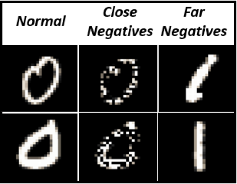
(a)

Figure 2: Sample postives, negatives and close negatives for MNIST digit 0 vs 1 experiment (OCLN).

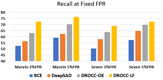
(a)

Figure 3: OCLN on Audio Commands: Comparison of Recall for key words — “Marvin” and “Seven” when the False Positive Rate(FPR) is fixed to be 3% and 5%. DROCC–LF is consistently about 10% more accurate than all the baseline

Wakeword Detection: Finally, we evaluate DROCC–LF on the practical problem of wakeword detection with low FPR against arbitrary OOD negatives. To this end, we identify a keyword, say “Marvin” from the audio commands dataset (Warden, 2018) as the positive class, and the remaining 34 keywords are labeled as the negative class. For training, we sample points uniformly at random from the above mentioned dataset. However, for evaluation, we sample positives from the train distribution, but negatives contain a few challenging OOD points as well. Sampling challenging negatives itself is a hard task and is the key motivating reason for studying the problem. So, we manually list close-by keywords to Marvin such as: Mar, Vin, Marvelous etc. We then generate audio snippets for these keywords via a speech synthesis tool with a variety of accents.

Figure  3 shows that for 3% and 5% FPR settings, DROCC–LF is significantly more accurate than the baselines. For example, with FPR=$3\%$, DROCC–LF is 10% more accurate than the baselines. We repeated the same experiment with the keyword: Seven, and observed a similar trend. See Table 9 in Appendix for the list of the close negatives which were synthesized for each of the keywords. In summary, DROCC–LF is able to generalize well against negatives that are “close” to the true positives even when such negatives were not supplied with the training data.

6 Conclusions

We introduced DROCC method for deep anomaly detection. It models normal data points using a low-dimensional manifold, and hence can compare close point via Euclidean distance. Based on this intuition, DROCC’s optimization is formulated as a saddle point problem which is solved via standard gradient descent-ascent algorithm. We then extended DROCC to ${\rm OCLN}$ problem where the goal is to generalize well against arbitrary negatives, assuming positive class is well sampled and a small number of negative points are also available. Both the methods perform significantly better than strong baselines, in their respective problem settings. For computational efficiency, we simplified the projection set for both the methods which can perhaps slow down the convergence of the two methods. Designing optimization algorithms that can work with the stricter set is an exciting research direction. Further, we would also like to rigorously analyse DROCC, assuming enough samples from a low-curvature manifold. Finally, as ${\rm OCLN}$ is an exciting problem that routinely comes up in a variety of real-world applications, we would like to apply DROCC–LF to a few high impact scenarios.

Acknowledgments

We are grateful to Aditya Kusupati, Nagarajan Natarajan, Sahil Bhatia and Oindrila Saha for helpful discussions and feedback. AR was funded by an Open Philanthropy AI Fellowship and Google PhD Fellowship in Machine Learning.

Appendix A ${\rm OCLN}$

A.1 DROCC–LF Proof

Proof of Proposition 1.

Recall the problem:

$$\min_{\tilde{x}}\|\tilde{x}-z\|^{2},\ s.t.,\ r^{2}\leq\|\tilde{x}-x\|_{\Sigma}^{2}\leq\gamma^{2}r^{2}.$$

Note that both the constraints cannot be active at the same time, so we can consider either $r^{2}\leq\|\tilde{x}-x\|_{\Sigma}^{2}$ constraint or $\|\tilde{x}-x\|_{\Sigma}^{2}\leq\gamma^{2}r^{2}$. Below, we give calculation when the former constraint is active, later’s proof follows along same lines.

Let $\tau\leq 0$ be the Lagrangian multiplier, then the Lagrangian function of the above problem is given by:

$$L(\tilde{x},\tau)=\|\tilde{x}-z\|^{2}+\tau(\|\tilde{x}-x\|_{\Sigma}^{2}-r^{2}).$$

Using KKT first-order necessary condition (Boyd & Vandenberghe, 2004), the following should hold for any optimal solution $\tilde{x},\tau$:

$$\nabla_{\tilde{x}}L(\tilde{x},\tau)=0.$$

That is,

$$\tilde{x}=(I+\tau\Sigma)^{-1}(z+\tau\cdot\Sigma x)=x+(I+\tau\cdot\Sigma)^{-1}\delta,$$

where $\delta=z-x$. This proves the first part of the lemma.

Now, by using primal and dual feasibility required by the KKT conditions, we have:

$$\min_{\tau\leq 0}\|\tilde{x}-z\|^{2},\ s.t.,\ \|\tilde{x}-x\|_{\Sigma}^{2}\geq r^{2},$$

where $\tilde{x}=(I+\tau\Sigma)^{-1}(z+\tau\cdot\Sigma x)=x+(I+\tau\cdot\Sigma)^{-1}\delta$. The lemma now follows by substituting $\tilde{x}$ above and by using the fact that $\Sigma$ is a diagonal matrix with $\Sigma(i,i)=\sigma_{i}$. ∎

A.2 DROCC–LF Algorithm

See Algorithm Box  2.

Algorithm 2 Training neural networks via DROCC–LF

Input: Training data $D=[(x_{1},y_{1}),(x_{2},y_{2}),\dots,(x_{n},y_{n})]$.

Parameters: Radius $r$, $\lambda\geq 0$, $\mu\geq 0$, step-size $\eta$, number of gradient steps $m$, number of initial training steps $n_{0}$.

Initial steps: For $B=1,\ldots n_{0}$

$X_{B}$: Batch of training inputs

$\theta=\theta-\text{Gradient-Step}\Big{(}\sum\limits_{\begin{subarray}{c}(x,y)\\ \in X_{B}\end{subarray}}\ell(f_{\theta}(x),y)\Big{)}$

DROCC steps: For $B=n_{0},\ldots n_{0}+N$

$X_{B}$: Batch of normal training inputs ($y=1$)

$\forall x\in X_{B}:h\sim\mathcal{N}(0,I_{d})$

Adversarial search: For $i=1,\ldots m$

1. $\ell(h)=\ell(f_{\theta}(x+h),-1)$

2. $h=h+\eta\frac{\nabla_{h}\ell(h)}{\|\nabla_{h}\ell(h)\|}$

3. $h=\text{Projection given by Proposition~{}\ref{prop:lfoc}}(\delta=h)$

$\ell^{itr}=\lambda\|\theta\|^{2}+\sum\limits_{\begin{subarray}{c}(x,y)\\ \in X_{B}\end{subarray}}\ell(f_{\theta}(x),y)+\mu\ell(f_{\theta}(x+h),-1)$

$\theta=\theta-\text{Gradient-Step}(\ell^{itr})$

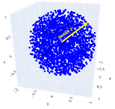
(a)

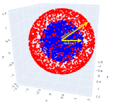
(b)

Figure 4: (a) Spherical manifold (a unit sphere) that captures the normal data distribution. Points are uniformly sampled from the volume of the unit sphere. (b) OOD points (red) are sampled on the surface of a sphere of varying radius. Table 6 shows AUC values with varying radius.

Table 6: Average AUC for Spherical manifold experiment (Section B.2). Normal points are sampled uniformly from the volume of a unit sphere and OOD points are sampled from the surface of a unit sphere of varying radius (See Figure 4b). Again DROCC outperforms all the baselines when the OOD points are quite close to the normal distribution.

Radius	Nearest Neighbor	OC-SVM	AutoEncoder	DeepSVDD	DROCC (Ours)
1.2	100 $\pm$ 0.00	92.00 $\pm$ 0.00	91.81 $\pm$ 2.12	93.26 $\pm$ 0.91	99.44 $\pm$ 0.10
1.4	100 $\pm$ 0.00	92.97 $\pm$ 0.00	97.85 $\pm$ 1.41	98.81 $\pm$ 0.34	99.99 $\pm$ 0.00
1.6	100 $\pm$ 0.00	92.97 $\pm$ 0.00	99.92 $\pm$ 0.11	99.99 $\pm$ 0.00	100.00 $\pm$ 0.00
1.8	100 $\pm$ 0.00	91.87 $\pm$ 0.00	99.98 $\pm$ 0.04	100.00 $\pm$ 0.00	100.00 $\pm$ 0.00
2.0	100 $\pm$ 0.00	91.83 $\pm$ 0.00	100 $\pm$ 0.00	100.00 $\pm$ 0.00	100.00 $\pm$ 0.00

Appendix B Synthetic Experiments

B.1 1-D Sine Manifold

In Section 5.1.1 we presented results on a synthetic dataset of 1024 points sampled from a 1-D sine wave (See Figure 1a). We compare DROCC to other anomaly detection methods by plotting the decision boundaries on this same dataset. Figure 5 shows the decision boundary for a) DROCC b) OC-SVM with RBF kernel c) OC-SVM with 20-degree polynomial kernel d) DeepSVDD. All methods are trained only on positive points from the 1-D manifold.

(a)

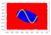
(b)

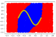
(c)

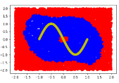
(d)

Figure 5: (a) Decision boundary of DROCC trained only on the positive points lying on the 1-D sine manifold in Figure 1a. Blue represents points classified as normal and red classified as abnormal. (b) Decision boundary of classical OC-SVM using RBF kernel and same experiment settings as in (a). Yellow sine wave just shows the underlying train data. (c) Decision boundary of classical OC-SVM using a 20-degree polynomial kernel. (d) Decision boundary of DeepSVDD.

We further evaluate these methods for varied sampling of negative points near the positive manifold. Negative points are sampled from a 1-D sine manifold vertically displaced in both directions (See Figure 6). Table 7 compares DROCC against various baselines on this dataset.

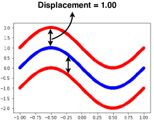
(a)

Figure 6: Illustration of the negative points sampled at various displacements of the sine wave; used for reporting the AUC values in the Table 7. In this figure, vertical displacement is 1.0. Blue represents the positive points (also the training data) and red represents the negative/OOD points

Table 7: Average AUC for the synthetic 1-D Sine Wave manifold experiment (Section B.1). Normal points are sampled from a sine wave and OOD points from a vertically displaced manifold (See Figure 6). The results demonstrate that only DROCC is able to capture the manifold tightly

Vertical Displacement	Nearest Neighbor	OC-SVM	AutoEncoder	DeepSVDD	DROCC (Ours)
0.2	100 $\pm$ 0.00	56.99 $\pm$ 0.00	52.48 $\pm$ 1.15	65.91 $\pm$ 0.64	96.80 $\pm$ 0.65
0.4	100 $\pm$ 0.00	68.84 $\pm$ 0.00	58.59 $\pm$ 0.61	78.18 $\pm$ 1.67	99.31 $\pm$ 0.80
0.6	100 $\pm$ 0.00	76.95 $\pm$ 0.00	66.59 $\pm$ 1.21	82.85 $\pm$ 1.96	99.92 $\pm$ 0.11
0.8	100 $\pm$ 0.00	81.73 $\pm$ 0.00	77.42 $\pm$ 3.62	86.26 $\pm$ 1.69	99.98 $\pm$ 0.01
1.0	100 $\pm$ 0.00	88.18 $\pm$ 0.00	86.14 $\pm$ 2.52	90.51 $\pm$ 2.62	100 $\pm$ 0.00
2.0	100 $\pm$ 0.00	98.56 $\pm$ 0.00	100 $\pm$ 0.00	100 $\pm$ 0.00	100 $\pm$ 0.00

B.2 Spherical Manifold

OC-SVM and DeepSVDD try to find a minimum enclosing ball for the whole set of positive points, while DROCC assumes that the true points low on a low dimensional manifold. We now test these methods on a different synthetic dataset: spherical manifold where the positive points are within a sphere, as shown in Figure 4a. Normal/Positive points are sampled uniformly from the volume of the unit sphere. Table 6 compares DROCC against various baselines when the OOD points are sampled on the surface of a sphere of varying radius (See Figure 4b). DROCC again outperforms all the baselines even in the case when minimum enclosing ball would suit the best. Suppose instead of neural networks, we were operating with purely linear models, then DROCC also essentially finds the minimum enclosing ball (for a suitable radius $r$). If $r$ is too small, the training doesn’t converge since there is no separating boundary). Assuming neural networks are implicitly regularized to find the simplest boundary, DROCC with neural networks also learns essentially a minimum enclosing ball in this case, however, at a slightly larger radius. Therefore, we get $100\%$ AUC only at radius $1.6$ rather than $1+\epsilon$ for some very small $\epsilon$.

(a)

(b)

(c)

Figure 7: Ablation Study : Variation in the performance DROCC when $r$ (with $\gamma=1$) is changed from the optimal value.

(a)

(b)

(c)

Figure 8: Ablation Study : Variation in the performance of DROCC with $\mu$ (1) which is the weightage given to the loss from adversarially sampled negative points

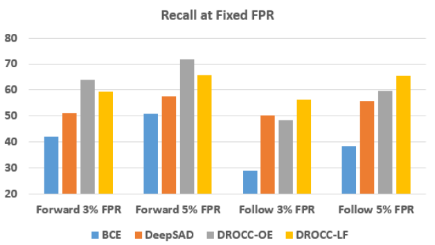
(a)

Figure 9: OCLN on Audio Commands: Comparison of Recall for key words — “Forward” and “Follow” when the False Positive Rate(FPR) is fixed to be 3% and 5%.

Table 8: Ablation Study on CIFAR-10: Sampling negative points randomly in the set $N_{i}(r)$ (DROCC–Rand) instead of gradient ascent (DROCC).

CIFAR Class	One-Class Deep SVDD	DROCC	DROCC–Rand
Airplane	61.7$\pm$4.1	81.66 $\pm$ 0.22	79.67 $\pm$ 2.09
Automobile	65.9$\pm$2.1	76.74 $\pm$ 0.99	73.48 $\pm$ 1.44
Bird	50.8$\pm$0.8	66.66 $\pm$ 0.96	62.76 $\pm$ 1.59
Cat	59.1$\pm$1.4	67.13 $\pm$ 1.51	67.33 $\pm$ 0.72
Deer	60.9$\pm$1.1	73.62 $\pm$ 2.00	56.09 $\pm$ 1.19
Dog	65.7$\pm$2.5	74.43 $\pm$ 1.95	65.88 $\pm$ 0.64
Frog	67.7$\pm$2.6	74.43 $\pm$ 0.92	74.82 $\pm$ 1.77
Horse	67.3$\pm$0.9	71.39 $\pm$ 0.22	62.08 $\pm$ 2.03
Ship	75.9$\pm$1.2	80.01 $\pm$ 1.69	80.04 $\pm$ 1.71
Truck	73.1$\pm$1.2	76.21 $\pm$ 0.67	70.80 $\pm$ 2.73

Table 9: Synthesized near-negatives for keywords in Audio Commands

Marvin	Forward	Seven	Follow
mar	for	one	fall
marlin	fervor	eleven	fellow
arvin	ward	heaven	low
marvik	reward	when	hollow
arvi	onward	devon	wallow

Table 10: Hyperparameters: Tabular Experiments

Dataset	Radius	$\mu$	Optimizer	Learning Rate	Adversarial Ascent Step Size
Abalone	3	1.0	Adam	$10^{-3}$	0.01
Arrhythmia	16	1.0	Adam	$10^{-4}$	0.01
Thyroid	2.5	1.0	Adam	$10^{-3}$	0.01

Table 11: Hyperparameters: CIFAR-10

Class	Radius	$\mu$	Optimizer	Learning Rate	Adversarial Ascent Step Size
Airplane	8	1	Adam	0.001	0.001
Automobile	8	0.5	SGD	0.001	0.001
Bird	40	0.5	Adam	0.001	0.001
Cat	28	1	SGD	0.001	0.001
Deer	32	1	SGD	0.001	0.001
Dog	24	0.5	SGD	0.01	0.001
Frog	36	1	SGD	0.001	0.01
Horse	32	0.5	SGD	0.001	0.001
Ship	28	0.5	SGD	0.001	0.001
Truck	16	0.5	SGD	0.001	0.001

Table 12: Hyperparameters: ImageNet

Class	Radius	$\mu$	Optimizer	Learning Rate	Adversarial Ascent Step Size
Tench	30	1	SGD	0.01	0.001
English_springer	16	1	SGD	0.001	0.001
Cassette_player	40	1	Adam	0.005	0.001
Chain_saw	20	1	SGD	0.01	0.001
Church	40	1	Adam	0.01	0.001
French_horn	20	1	SGD	0.05	0.001
Garbage_truck	30	1	Adam	0.005	0.001
Gas_pump	30	1	Adam	0.01	0.001
Golf_ball	30	1	SGD	0.01	0.001
Parachute	12	1	Adam	0.001	0.001

Table 13: Hyperparameters: Timeseries Experiments

Dataset	Radius	$\mu$	Optimizer	Learning Rate	Adversarial Ascent Step Size
Epilepsy	10	0.5	Adam	$10^{-5}$	0.1
Audio Commands	16	1.0	Adam	$10^{-3}$	0.1

Table 14: Hyperparameters: LFOC Experiments

Keyword	Radius	$\mu$	Optimizer	Learning Rate	Adversarial Ascent Step Size
Marvin	32	1	Adam	0.001	0.01
Seven	36	1	Adam	0.001	0.01
Forward	40	1	Adam	0.001	0.01
Follow	20	1	Adam	0.0001	0.01

Appendix C LFOC Supplementary Experiments

In Section 5.2.1, we compared DROCC–LF with various baselines for the ${\rm OCLN}$ task where the goal is to learn a classifier that is accurate for both the positive class and the arbitrary OOD negatives. Figure 9 compares the recall obtained by different methods on 2 keywords ”Forward” and ”Follow” with 2 different FPR. Table 9 lists the close negatives which were synthesized for each of the keywords.

Appendix D Ablation Study

D.1 Hyper-Parameters

Here we analyze the effect of two important hyper-parameters — radius $r$ of the ball outside, which we sample negative points (set $N_{i}(r)$), and $\mu$ which is the weightage given to the loss from adversarially generated negative points (See Equation 1). We set $\gamma=1$ and hence recall that the negative points are sampled to be at a distance of r from the positive points.

Figure 7a, 7b and 7c show the performance of DROCC with varied values of $r$ on the CIFAR-10 dataset. The graphs demonstrate that sampling negative points quite far from the manifold (setting $r$ to be very large), causes a drop in the accuracy since now DROCC would be covering the normal data manifold loosely causing high false positives. At the other extreme, if the radius is set too small, the decision boundary could be too close to the positive and hence lead to overfitting and difficulty in training the neural network. Hence, setting an appropriate radius value is very critical for the good performance of DROCC.

Figure 8a, 8b and 8c show the effect of $\mu$ on the performance of DROCC on CIFAR-10.

D.2 Importance of gradient ascent-descent technique

In the Section 1 we formulated the DROCC’s optimization objective as a saddle point problem (Equation 1). We adopted the standard gradient descent-ascent technique to solve the problem replacing the $\ell_{p}$ ball with $N_{i}(r)$. Here, we present an analysis of DROCC without the gradient ascent part i.e., we now sample points at random in the set of negatives $N_{i}(r)$. We call this formulation as DROCC–Rand. Table 8 shows the drop in performance when negative points are sampled randomly on the CIFAR-10, hence emphasizing the importance of gradient ascent-descent technique. Since $N_{i}(r)$ is high dimensional, random sampling does not find points close enough to manifold of positive points.

Appendix E Experiment details and Hyper-Parameters for Reproducibility

E.1 Tabular Datasets

Following previous work, we use a base network consisting of a single fully-connected layer with 128 units for the deep learning baselines. For the classical algorithms, the features are input to the model. Table 10 lists all the hyper-parameters for reproducibility.

E.2 CIFAR-10

DeepSVDD uses the representations learnt in the penultimate layer of LeNet (LeCun et al., 1998) for minimizing their one-class objective. To make a fair comparison, we use the same base architecture. However, since DROCC formulates the problem as a binary classification task, we add a final fully connected layer over the learned representations to get the binary classification scores. Table 11 lists the hyper-parameters which were used to run the experiments on the standard test split of CIFAR-10.

E.3 ImageNet-10

MobileNetv2 (Sandler et al., 2018a) was used as the base architecture for DeepSVDD and DROCC. Again we use the representations from the penultimate layer of MobileNetv2 for optimizing the one-class objective of DeepSVDD. The width multiplier for MobileNetv2 was set to be 1.0. Table 12 lists all the hyper-parameters.

E.4 Time Series Datasets

To keep the focus only on comparing DROCC against the baseline formulations for OOD detection, we use a single layer LSTM for all the experiments on Epileptic Seizure Detection, and the Audio Commands dataset. The hidden state from the last time step is used for optimizing the one class objective of DeepSVDD. For DROCC we add a fully connected layer over the last hidden state to get the binary classification scores. Table 13 lists all the hyper-parameters for reproducibility.

E.5 LFOC Experiments on Audio Commands

For the Low-FPR classification task, we use keywords from the Audio Commands dataset along with some synthesized near-negatives. The training set consists of 1000 examples of the keyword and 2000 randomly sampled examples from the remaining classes in the dataset. The validation and test set consist of 600 examples of the keyword, the same number of words from other classes of Audio Commands dataset and an extra synthesized 600 examples of close negatives of the keyword (see Table 9) A single layer LSTM, along with a fully connected layer on top on the hidden state at last time step was used. Similar to experiments with DeepSVDD, DeepSAD uses the hidden state of the final timestep as the representation in the one-class objective. An important aspect of training DeepSAD is the pretraining of the network as the encoder in an autoencoder. We also tuned this pretraining to ensure the best results.

References

- Aggarwal (2016) Aggarwal, C. C. Outlier Analysis. Springer Publishing Company, Incorporated, 2nd edition, 2016. ISBN 3319475770.
- Andrzejak et al. (2001) Andrzejak, R. G., Lehnertz, K., Mormann, F., Rieke, C., David, P., and Elger, C. E. Indications of nonlinear deterministic and finite-dimensional structures in time series of brain electrical activity: Dependence on recording region and brain state. Physical Review E, 64(6), 2001.
- Bergman & Hoshen (2020) Bergman, L. and Hoshen, Y. Classification-based anomaly detection for general data. In International Conference on Learning Representations (ICLR), 2020.
- Boyd & Vandenberghe (2004) Boyd, S. and Vandenberghe, L. Convex Optimization. Cambridge University Press, USA, 2004. ISBN 0521833787.
- Breunig et al. (2000) Breunig, M. M., Kriegel, H.-P., Ng, R. T., and Sander, J. Lof: identifying density-based local outliers. In Proceedings of the 2000 ACM SIGMOD international conference on Management of data, pp. 93–104, 2000.
- Caron et al. (2018) Caron, M., Bojanowski, P., Joulin, A., and Douze, M. Deep clustering for unsupervised learning of visual features. In Proceedings of the European Conference on Computer Vision (ECCV), pp. 132–149, 2018.
- Chandola et al. (2009) Chandola, V., Banerjee, A., and Kumar, V. Anomaly detection: A survey. ACM Computing Surveys (CSUR), 41(3), 2009.
- Das et al. (2018) Das, S., Islam, M. R., Jayakodi, N. K., and Doppa, J. R. Active anomaly detection via ensembles, 2018.
- Deng et al. (2009) Deng, J., Dong, W., Socher, R., Li, L.-J., Li, K., and Fei-Fei, L. Imagenet: A large-scale hierarchical image database. In IEEE Conference on Computer Vision and Pattern Recognition (CVPR), 2009.
- (10) Dennis, D. K., Gaurkar, Y., Gopinath, S., Goyal, S., Gupta, C., Jain, M., Kumar, A., Kusupati, A., Lovett, C., Patil, S. G., Saha, O., and Simhadri, H. V. EdgeML: Machine Learning for resource-constrained edge devices. URL https://github.com/Microsoft/EdgeML.
- Dua & Graff (2017) Dua, D. and Graff, C. UCI machine learning repository, 2017. URL http://archive.ics.uci.edu/ml.
- Golan & El-Yaniv (2018) Golan, I. and El-Yaniv, R. Deep anomaly detection using geometric transformations. In Advances in Neural Information Processing Systems (NeurIPS), 2018.
- Goldstein & Uchida (2016) Goldstein, M. and Uchida, S. A comparative evaluation of unsupervised anomaly detection algorithms for multivariate data. PLOS ONE, 11(4), 2016.
- Gu et al. (2019) Gu, X., Akoglu, L., and Rinaldo, A. Statistical analysis of nearest neighbor methods for anomaly detection. In Advances in Neural Information Processing Systems (NeurIPS), 2019.
- Hendrycks et al. (2019a) Hendrycks, D., Mazeika, M., and Dietterich, T. Deep anomaly detection with outlier exposure. In International Conference on Learning Representations (ICLR), 2019a.
- Hendrycks et al. (2019b) Hendrycks, D., Mazeika, M., Kadavath, S., and Song, D. Using self-supervised learning can improve model robustness and uncertainty. In Advances in Neural Information Processing Systems (NeurIPS), 2019b.
- Krizhevsky (2009) Krizhevsky, A. Learning multiple layers of features from tiny images, 2009.
- Kusupati et al. (2018) Kusupati, A., Singh, M., Bhatia, K., Kumar, A., Jain, P., and Varma, M. Fastgrnn: A fast, accurate, stable and tiny kilobyte sized gated recurrent neural network. In Advances in Neural Information Processing Systems, pp. 9017–9028, 2018.
- Lakhina et al. (2004) Lakhina, A., Crovella, M., and Diot, C. Diagnosing network-wide traffic anomalies. SIGCOMM Comput. Commun. Rev., 34(4), 2004.
- LeCun et al. (1998) LeCun, Y., Bottou, L., Bengio, Y., and Haffner, P. Gradient-based learning applied to document recognition. Proceedings of the IEEE, 86(11), 1998.
- Li et al. (2018) Li, D., Chen, D., Goh, J., and kiong Ng, S. Anomaly detection with generative adversarial networks for multivariate time series, 2018.
- Liu et al. (2008) Liu, F. T., Ting, K. M., and Zhou, Z.-H. Isolation forest. In Proceedings of the 2008 Eighth IEEE International Conference on Data Mining, 2008.
- Madry et al. (2018) Madry, A., Makelov, A., Schmidt, L., Tsipras, D., and Vladu, A. Towards deep learning models resistant to adversarial attacks. In International Conference on Learning Representations (ICLR), 2018.
- Malhotra et al. (2016) Malhotra, P., Ramakrishnan, A., Anand, G., Vig, L., Agarwal, P., and Shroff, G. Lstm-based encoder-decoder for multi-sensor anomaly detection, 2016. URL https://arxiv.org/abs/1607.00148.
- Nguyen et al. (2019) Nguyen, D. T., Lou, Z., Klar, M., and Brox, T. Anomaly detection with multiple-hypotheses predictions. In International Conference on Machine Learning (ICML), 2019.
- Pless & Souvenir (2009) Pless, R. and Souvenir, R. A survey of manifold learning for images. IPSJ Transactions on Computer Vision and Applications, 1, 2009.
- Rayana (2016) Rayana, S. ODDS library, 2016. URL http://odds.cs.stonybrook.edu.
- Ruff et al. (2018) Ruff, L., Vandermeulen, R., Goernitz, N., Deecke, L., Siddiqui, S. A., Binder, A., Müller, E., and Kloft, M. Deep one-class classification. In International Conference on Machine Learning (ICML), 2018.
- Ruff et al. (2020) Ruff, L., Vandermeulen, R. A., Görnitz, N., Binder, A., Müller, E., Müller, K.-R., and Kloft, M. Deep semi-supervised anomaly detection. In International Conference on Learning Representations (ICLR), 2020.
- Sakurada & Yairi (2014) Sakurada, M. and Yairi, T. Anomaly detection using autoencoders with nonlinear dimensionality reduction. In Proceedings of the MLSDA 2014 2nd Workshop on Machine Learning for Sensory Data Analysis, 2014.
- Sandler et al. (2018a) Sandler, M., Howard, A., Zhu, M., Zhmoginov, A., and Chen, L.-C. Mobilenetv2: Inverted residuals and linear bottlenecks, 2018a. URL https://arxiv.org/abs/1801.04381.
- Sandler et al. (2018b) Sandler, M., Howard, A., Zhu, M., Zhmoginov, A., and Chen, L.-C. Mobilenetv2: Inverted residuals and linear bottlenecks. In IEEE Conference on Computer Vision and Pattern Recognition (CVPR), 2018b.
- Schlegl et al. (2017a) Schlegl, T., Seeböck, P., Waldstein, S. M., Schmidt-Erfurth, U., and Langs, G. Unsupervised anomaly detection with generative adversarial networks to guide marker discovery. In International conference on information processing in medical imaging, pp. 146–157. Springer, 2017a.
- Schlegl et al. (2017b) Schlegl, T., Seeböck, P., Waldstein, S. M., Schmidt-Erfurth, U., and Langs, G. Unsupervised anomaly detection with generative adversarial networks to guide marker discovery. Information Processing in Medical Imaging, 2017b.
- Schölkopf et al. (1999) Schölkopf, B., Williamson, R., Smola, A., Shawe-Taylor, J., and Platt, J. Support vector method for novelty detection. In Proceedings of the 12th International Conference on Neural Information Processing Systems, 1999.
- Seeböck et al. (2016) Seeböck, P., Waldstein, S., Klimscha, S., Gerendas, B. S., Donner, R., Schlegl, T., Schmidt-Erfurth, U., and Langs, G. Identifying and categorizing anomalies in retinal imaging data. arXiv preprint arXiv:1612.00686, 2016.
- Srivastava et al. (2015) Srivastava, N., Mansimov, E., and Salakhudinov, R. Unsupervised learning of video representations using lstms. In International Conference on Machine Learning (ICML), 2015.
- Tax & Duin (2004) Tax, D. M. and Duin, R. P. Support vector data description. Machine Learning, 54(1), 2004.
- Warden (2018) Warden, P. Speech commands: A dataset for limited-vocabulary speech recognition, 2018. URL https://arxiv.org/abs/1804.03209.
- Zhai et al. (2016) Zhai, S., Cheng, Y., Lu, W., and Zhang, Z. Deep structured energy based models for anomaly detection. In International Conference on Machine Learning (ICML), 2016.
- Zong et al. (2018) Zong, B., Song, Q., Min, M. R., Cheng, W., Lumezanu, C., Cho, D., and Chen, H. Deep autoencoding gaussian mixture model for unsupervised anomaly detection. In International Conference on Learning Representations, 2018. URL https://openreview.net/forum?id=BJJLHbb0-.