TNOs are Cool! A Survey of the transneptunian Region

The goal of this work is to determine the physical characteristics of resonant, detached and scattered disk objects in the trans-Neptunian region, observed mainly in the framework of the “TNOs are Cool” Herschel Open Time Key Programme. Based on thermal emission measurements with the Herschel/PACS and Spitzer/MIPS instruments, we determine size, albedo, and surface thermal properties for 23 objects using radiometric modeling techniques. This is the first analysis in which the physical properties of objects in the outer resonances are determined for a notable sample. In addition to the results for individual objects, we compared these characteristics with the bulk properties of other populations of the trans-Neptunian region. The newly analyzed objects show a large variety of beaming factors, indicating a diversity of thermal properties, and in general they follow the albedo-color clustering identified earlier for Kuiper belt objects and Centaurs, further strengthening the evidence for a compositional discontinuity in the young Solar System.

1 Introduction

Trans-Neptunian objects in mean motion resonance with Neptune (RTNOs; see, e.g., Gladman et al., 2012, and references therein) show a dynamical behavior that their resonance angle $\phi_{jk}$ = j$\lambda$ - k$\lambda_{N}$ - (j-k)$\varpi$ (where $\lambda$ is the longitude of object, $\lambda_{N}$ the longitude of Neptune, and $\varpi$ the longitude of perihelion of the RTNO, for a specific j:k resonance) cannot have all values between 0° and 360°. Typically, the resonance angle is confined to a mean value with some relatively small libration amplitude. An important feature of the resonances is that they may provide protection against perturbations and allow large eccentricity orbits to survive for the age of the Solar System. Even so, the chaotic nature of the resonance border allows temporary trapping of objects near the border of the resonance, and nearly resonant objects can escape into a dynamical regime where perturbations may direct them out of the Kuiper belt toward the inner Solar System. Resonant objects also serve as a diagnostic tool of the planetary migration era. Current population estimates of RTNOs are consistent with a scenario that they were likely put in place in the resonances during the planet migration era at the end of the giant-planet formation process (Gladman et al., 2012). RTNOs show dynamical characteristics (e.g., inclination distribution) different from those of the classical Kuiper belt, but may be connected to the scattered disk population (Gomes et al., 2008), objects on high eccentricity orbits with perihelia beyond Neptune, and semi-major axes beyond the 2:1 resonance. Recent studies (Yu et al., 2018) indicate that a significant fraction of all scattered objects are transiently stuck in mean motion resonances, suggesting that these objects originated from the same single population.

The Outer Solar System Origins Survey (OSSOS Bannister et al., 2018) recently provided a significant increase in the number of RTNOs, adding 313 new objects of which 132 are plutinos. This survey also detected two objects in the distant 9:1 resonance (Volk et al., 2018) that may have originated in the scattered population, and that became trapped in this resonance within the last $\sim$1 Gyr, but could also be remnants of a larger, primordial population.

In addition to dynamical properties Sheppard (2012) obtained broad-band color of 58 resonant objects, with significantly different color distributions in the different resonances. For example, those in the 5:3 and 7:4 resonances are dominated by ultra-red material, similar to that in the cold classical belt. Objects in the inner 4:3 and distant 5:2 resonances show mostly moderate red colors, similar to the scattered and detached populations, while the 2:1 and 3:2 resonances show a wide range of colors. Apart from the dynamical properties, color, albedo, and size are very crucial physical characteristics of these objects; however, they can be determined only when thermal emission data or occultation measurements are available.

In the framework of the “TNOs are Cool”: A survey of the trans-Neptunian region, a Herschel Open Time Key Programme (Müller et al., 2009), several papers have been published on the physical characteristics of Centaurs and trans-Neptunian objects in population-specific papers, and in other papers concentrating on specifically selected objects (Pál et al., 2012; Fornasier et al., 2013) or on the general properties of these small bodies (Lellouch et al., 2013). These papers used thermal emission data obtained with the PACS photometer camera of the Herschel Space Observatory in the far-infrared, at 70, 100, and 160 $\mu$m. The population-specific papers included the Centaurs (Duffard et al., 2014), classical Kuiper belt objects (Vilenius et al., 2012, 2014), plutinos (Mommert et al., 2012), some scattered disk and detached objects (Santos-Sanz et al., 2012), and also the members of the Haumea collisional family (Vilenius et al., 2018).

Using these data, in particular the size and albedo derived using radiometric models that were supplemented by color information, Lacerda et al. (2014) found evidence for a compositional discontinuity in the early Solar System, identifying two distinct types of planetary bodies: objects with dark (geometric albedo of p_V $\approx$ 0.05) and neutrally colored surfaces, or with bright (p_V $\approx$ 0.15) and red surfaces. Objects in relic populations (cold classicals, detached objects, and outer resonances, i.e., the 2:1 mean-motion resonance and beyond) show exclusively bright-red surfaces, while objects in dynamically less stable populations (Centaurs, plutinos, scattered disk object, and hot classicals) contain a mixture of bright-red and dark-neutral surfaces.

The largest set of RTNOs with reliable size and albedo information available are the plutinos. Mommert et al. (2012) derived these physical characteristics for 18 objects as part of the “TNOs Are Cool” program. They found sizes ranging from 150 to 730 km and geometric albedos varying between 0.04 and 0.28, with an average albedo of 0.08$\pm$0.03, similar to the mean albedo of Centaurs, Jupiter family comets, and other TNOs except cold classicals and detached objects. Based on these results, the cumulative power law of the size distribution in this dynamical group is q = 2 between sizes of 120 to 400 km, and q = 3 for larger objects.

In a similar study (Santos-Sanz et al., 2012) investigated 15 scattered disk and detached objects and found notably different albedos between the scattered disk and detached subpopulations (mean geometric albedos of 6.9% and 17%, respectively) .

Data from both studies were incorporated in the paper by Lacerda et al. (2014), with additional objects from the incomplete Herschel sample of RTNOs in non-3:2 resonances and additional scattered disk objects from Lellouch et al. (2013). A recent summary of thermal infrared observations of Centaurs and trans-Neptunian objects can be found in Müller et al. (2019).

In this paper we present the results of an investigation similar to those in the “TNOs are Cool” sample papers, focusing on Herschel/PACS observations of as-yet unpublished resonant and scattered disk objects. We derive size and albedo from Herschel/PACS measurements and derive radiometric models of 15 resonant, 7 scattered disk, and 1 detached object, in some cases supplemented by data from the MIPS camera of the Spitzer Space Telescope, not presented in earlier papers. We also reconsidered the data of a scattered disk and a detached object with inconsistent flux densities or problematic radiometric fits in previous papers, derived new flux densities using the final version of our data reduction pipeline, and obtained updated radiometric size and albedo estimates. Our results are then compared with color-albedo data of the trans-Neptunian dynamical populations derived in previous papers.

2 Observations, data reduction, and radiometric modeling

2.1 Herschel-PACS data

All Herschel-PACS measurements presented in this paper as new data were taken in scan-map mode with the PACS photometer arrays, following the observation strategy of the “TNOs are Cool” Open Time Key Programme (Müller et al., 2009; Vilenius et al., 2012; Kiss et al., 2014). Reduction of PACS photometer data is performed using the latest version of the “TNOs are Cool” pipeline. Both the key program observation strategies and the main characteristics and features of the pipeline are summarized in Kiss et al. (2014).

All Herschel/PACS measurements presented here as new reduction followed the same observation strategy: the target is observed at two epochs, typically separated by a day, and the data of the two epochs are combined to allow for optimal background elimination. At each epoch we observed the target with two 70/160 $\mu$m and two 100/160 $\mu$m filter astronomical observation requests (AORs), corresponding to 70° and 110° scan direction orientations. Altogether we obtained eight AORs per target, and correspondingly eight individual observation idendifiers (OBSIDs; see Table 1). Then the data of these OBSIDs are combined to obtain the final products. We note that 2003 UY₁₁₇ was measured with Herschel/PACS using the 70/160 $\mu$m filter combination only, while all other targets were observed with both filter combinations.

We used the following main settings to obtain Level-2 flux-calibrated PACS scan maps from the raw PACS measurements:

• Scan legs are extended based on the slew speed 15 and 25″ $s^{-1}$, around the commanded 20″ $s^{-1}$ scan speed.

• High pass filtering with filter width of 8, 9, and 16 is used at 70, 100, and 160 $\mu$m, respectively (high pass filter width sets the number of frames [2n+1] used for median subtraction from the detector timeline; see Popesso et al. 2012 and Balog et al. 2014 for a detailed description of the method).

• Pixel masking is used above 2$\sigma$, and at the source position with 2$\times$FWHM radius

• Second-level deglitching is applied with nsigma = 30, the sigma-clipping parameter of this deglitching method working on the map level (see the PACS Data Reduction Guide (2015) for more details).

• Correction for the apparent motion of the target is not applied to allow an optimal evaluation of the sky background using multiple measurements.

• The drizzle method is used to project the time-line data and to produce the single maps using the photProject() task in HIPE, with a pixel fraction parameter of 1.0.

As a standard setting for all “TNOs are Cool” data products we use pixel sizes of 1$\aas@@fstack{\prime\prime}$1, 1$\aas@@fstack{\prime\prime}$4, and 2$\aas@@fstack{\prime\prime}$1 in the PACS 70, 100, and 160 $\mu$m bands, different from the “physical” pixel sizes of 3.2″ and 6.4″ for the blue and red detectors, respectively. This allows an optimal sampling of the respective point spread functions (see Kiss et al., 2014). Our flux calibration is based on a set of standard stars with the same basic data reduction settings as in the case of our Solar System targets. Determination of the photometric uncertainty in scan maps is performed using the implanted source method, as described in Kiss et al. (2014). The flux densities of Solar System targets are derived from the double-differential products (see Kiss et al., 2014, for details). These double-differential images, as well as co-added and simple differential images, are available in the Herschel Science Archive as User Provided Data Products (UPDPs), along with a detailed description of the processing steps and the data products (UPDP Release Note Version 1.0, May 5, Kiss et al., 2017). The summary of the observations, as well as the derived in-band flux densities, are measured with the specific instrument–filter combinations) are presented in Table 1.

We reanalyzed the PACS observations of two targets from Santos-Sanz et al. (2012), 1999 KR₁₆ and 2005 QU₁₈₂. In both cases in the earlier evaluation the 100 $\mu$m flux densities were inconsistently low compared with the 70 and 160 $\mu$m flux densities. While there are some differences between the Santos-Sanz et al. (2012) and the present calibration and data reduction (e.g., different HIPE version, absolute calibration) the main difference is that in Santos-Sanz et al. (2012) a different kind of data product, namely supersky-subtracted images were used for final photometry. As discussed in Kiss et al. (2014, 2016b), double-differential (DDIFF) maps are superior in obtaining accurate and reliable photometry compared with supersky-subtracted maps, and we used these DDIFF maps for 1999 KR₁₆ and 2005 QU₁₈₂, reduced with the latest version of our pipeline (Kiss et al., 2016b). The supersky-subtracted images are more sensitive to the presence of background sources close to the target at one of the epochs considered. This was the case for the PACS measurements of both targets. By using these DDIFF images the 100 $\mu$m flux densities are now consistent with those in the two other bands, as confirmed by the subsequent radiometric modeling (see Sect. 3).

In addition to these objects, updated flux densities of 2007 UK₁₂₆, along with albedo and size derived from a combination of radiometric modeling and occultation data, are available in Schindler et al. (2017). Similarly, a revised radiometric model is available for 2007 OR₁₀ in Kiss et al. (2019). All Herschel/PACS data are available in the “Small Bodies: Near and Far” database of thermal infrared observations of Solar System small bodies (Kiss et al., 2019; Szakáts et al., 2020).

Table 1: Herschel in-band fluxes at all three PACS bands for the “new” objects, and for two objects with updated fluxes, presented in this work. Column headings (from left to right): object name; Dynamical classification (Res: resonant, SDO: scattered disk object, DO: detached object); OBSID: observation identifiers in the Herschel Science Archive; t_OBS: total duration of the two visits; JD: measurement mid-time in Julian date; r_h: heliocentric distance; $\Delta$: observer-to-target distance; $\alpha$: phase angle; F₇₀, F₁₀₀, and F₁₆₀: in-band flux densities obtained in the PACS 70, 100, and 160 $\mu$m bands, respectively. Upper limits correspond to 2$\sigma$ uncertainties derived with the implanted source method (Vilenius et al., 2014; Kiss et al., 2014). *: target from Santos-Sanz et al. (2012) and **: target from Vilenius et al. (2018) reanalyzed with the latest version of our data reduction pipeline.

Object	Dyn.	OBSID	tOBS	JD	rh	$\Delta$	$\alpha$	F70	F100	F160
	cl.		(sec)	(day)	(AU)	(AU)	(deg)	(mJy)	(mJy)	(mJy)
(26181) 1996 GQ21	SDO	1342212818/…821	5656	2455579.43	41.6056	41.9751	1.26	4.51$\pm$1.01	6.78$\pm$1.28	7.53$\pm$2.15
		1342213075/…078	5656	2455580.23	41.6063	41.9628	1.26
(523588) 2000 CN105	Res 9:5	1342197691/…694	3400	2455351.20	46.5639	46.6134	1.25	$<$ 1.31	$<$ 1.50	$<$ 1.63
		1342197781/…784	3400	2455352.41	46.5641	46.6340	1.25
(82075) 2000 YW134	Res 8:3	1342196008/…011	4528	2455325.61	44.2099	44.3812	1.30	4.88$\pm$1.07	5.13$\pm$1.47	4.88$\pm$2.13
		1342196133/…036	4528	2455326.83	44.2105	44.4024	1.29
		1342187074	5666	2455154.17	44.1263	43.8338	1.25		–
(82155) 2001 FZ173	SDO	1342236630/…633	4528	2455933.26	32.4131	32.5753	1.72	8.51$\pm$1.54	7.91$\pm$1.77	5.01$\pm$2.46
		1342236908/…011	4528	2455934.17	32.4132	32.5596	1.73
(139775) 2001 QG298	Plutino	1342213211/…214	5656	2455585.66	31.7619	32.1381	1.64	$<$ 0.913	$<$ 1.19	$<$ 2.00
		1342213266/…269	5656	2455586.32	31.7619	32.1489	1.64
2001 QX322	SDO	1342211619/…622	5656	2455557.80	41.3329	41.0520	1.32	$<$ 0.99	$<$ 1.06	$<$ 1.51
		1342211807/…010	5656	2455558.58	41.3336	41.0646	1.32
(42301) 2001 UR163	SDO	1342199507/…510	2272	2455378.59	50.9591	51.3267	1.07	2.88$\pm$1.37	$<$1.69	$<$3.09
		1342199650/…653	2272	2455380.07	50.9601	51.3042	1.08
(126154) 2001 YH140	Res 5:3	1342206036/…039	3400	2455477.34	36.6150	36.9327	1.49	5.08$\pm$1.40	3.67$\pm$1.70	$<$1.95
		1342206056/…059	3400	2455478.10	36.6151	36.9203	1.49
		1342187062	5666	2455153.28	36.5768	36.1686	1.44		–
(119878) 2002 CY224	Res 12:5	1342195506/…509	3400	2455311.51	37.2072	36.8614	1.47	$<$ 1.59	$<$ 1.78	$<$ 2.1
		1342195610/…613	3400	2455313.49	37.2082	36.8945	1.49
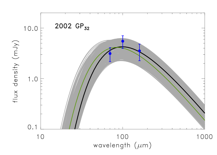
2002 GP32	Res 5:2	1342204144/…147	3400	2455448.42	32.1569	32.3768	1.76	3.09$\pm$0.95	5.43$\pm$1.53	3.58$\pm$1.29
		1342204204/…207	3400	2455449.05	32.1570	32.3875	1.75
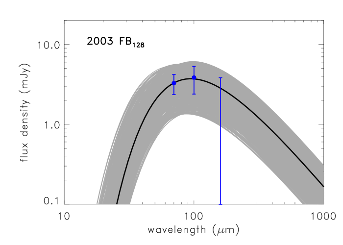
(133067) 2003 FB128	Plutino	1342237146/…149	4528	2455938.19	34.2390	34.6867	1.47	3.22$\pm$0.90	3.80$\pm$1.44	$<$ 1.94
		1342237226/…229	4528	2455938.85	34.2395	34.6769	1.47
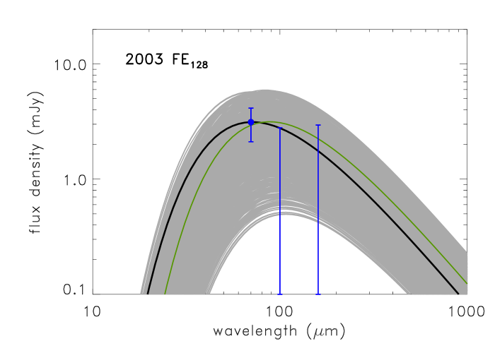
(469505) 2003 FE128	Res 2:1	1342237150/…153	5656	2455938.25	35.8635	36.3139	1.40	3.08$\pm$1.00	$<$ 1.39	$<$ 2.51
		1342237230/…033	5656	2455938.91	35.8635	36.3037	1.41
(143707) 2003 UY117	Res 5:2	1342238745/…746	3392	2455965.35	32.8901	33.1340	1.67	6.13$\pm$0.76	–	$<$ 2.16
		1342238790/…791	3392	2455965.98	32.8903	33.1447	1.66
(455502) 2003 UZ413	Plutino	1342212760/…763	2272	2455578.11	42.6153	42.2946	1.26	21.49$\pm$1.45	17.02$\pm$1.71	14.82$\pm$3.53
		1342212858/…861	2272	2455579.85	42.6162	42.3239	1.27
(450265) 2003 WU172	Plutino	1342250794/…797	2836	2456180.54	29.6443	29.8432	1.91	6.29$\pm$1.40	9.44$\pm$1.38	3.92$\pm$1.87
		1342250830/…833	2836	2456181.36	29.6441	29.8292	1.92
(175113) 2004 PG115	SDO	1342219009/…012	2256	2455670.53	36.9594	37.3635	1.43	6.68$\pm$2.39	8.43$\pm$3.03	$<$ 3.15
		1342219048/…051	2256	2455671.09	36.9596	37.3554	1.44
(145451) 2005 RM43	SDO	1342202281/…284	2272	2455417.29	35.4298	35.6640	1.60	15.20$\pm$1.18	16.55$\pm$2.87	14.79$\pm$2.41
		1342202320/…323	2272	2455417.99	35.4301	35.6527	1.60
(308379) 2005 RS43	Res 2:1	1342213502/…505	4528	2455592.24	42.4029	42.7677	1.24	3.09$\pm$0.94	3.45$\pm$1.46	$<$1.83
		1342213558/…561	4528	2455593.00	42.4033	42.7805	1.24
(40314) 1999 KR16**	DO	1342212814/…817	5844	2455579.36	35.7593	36.0633	1.51	7.61$\pm$1.44	5.21$\pm$2.29	$<$ 1.98
		1342213071/…074	5844	2455580.16	35.7589	36.0497	1.51
(303775) 2005 QU182*	SDO	1342212619/…622	2460	2455576.11	48.8994	49.1349	1.13	4.41$\pm$1.28	6.94$\pm$2.11	$<$ 2.73
		1342212696/…699	2460	2455577.08	48.9008	49.1522	1.12

2.2 Spitzer/MIPS data

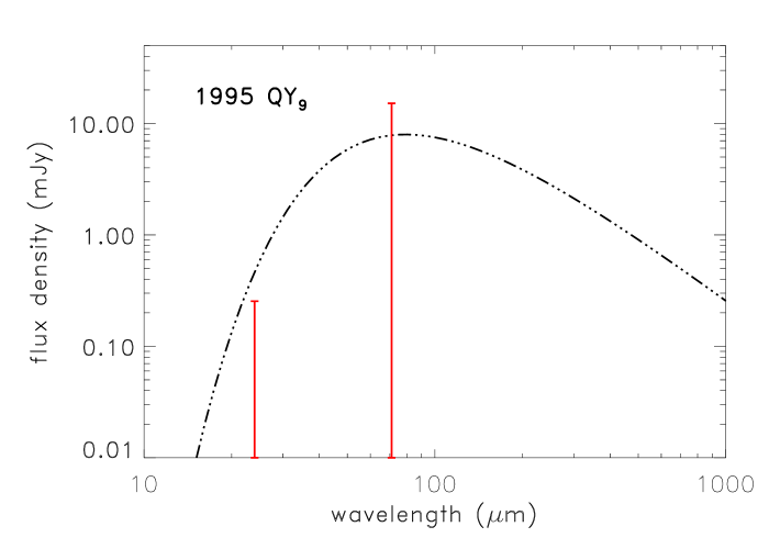
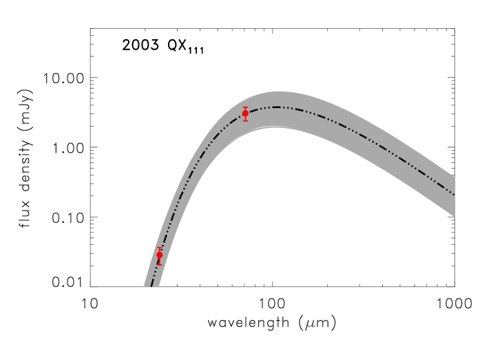
Spitzer/MIPS measurements were reduced using the same pipeline as was used for the reduction of MIPS data of Centaurs and trans-Neptunian objects by Mueller et al. (2012) and Stansberry et al. (2008, 2012). The MIPS instrument team data analysis tools (Gordon et al., 2005) were used to produce flux-calibrated images for each band, and the contribution of background objects were subtracted (see Stansberry et al. 2008). Aperture photometry was performed on the original images and on the final images, and the final flux values were obtained using the aperture corrections by Gordon et al. (2007) and Engelbracht et al. (2007). The flux densities obtained are presented in Table 2. In four cases Spitzer/MIPS flux densities were obtained in addition to the PACS fluxes (upper five rows in Table 2). We have three targets with Spitzer data only. In these cases the same methods were applied as in the case of PACS only and PACS/MIPS combined measurements. Spitzer-only targets were the plutinos 1995 QY₉ and 2003 QX₁₁₁ and the Neptune trojan 2001 QR₃₂₂.

Table 2: Spitzer observations summary. Columns headings (from left to right): objects name; dynamical class; Spitzer observation identifier; observation date; heliocentric distance; target-to-observer distance; phase angle; Spitzer/MIPS 24 $\mu$m in-band flux density; Spitzer/MIPS 71 $\mu$m in-band

flux density. object Dyn. AORkeys JD r_h $\Delta$ $\alpha$ F₂₄ F₇₁ cl. (day) (AU) (AU) (deg) (mJy) (mJy) 1996 GQ₂₁ SDO 9038848 2453222.29 39.937 39.977 1.46 — $<$ 3.537 2000 YW₁₃₄ Res 8:3 25234688, 944, 25235200 2454829.68 43.967 43.604 1.24 0.032 $\pm$ 0.015 $<$ 1.29 9039872 2453108.12 43.197 42.988 1.30 — 4.676 $\pm$ 2.186 2001 QX₃₂₂ SDO 9036544 2453368.70 39.617 39.393 1.42 — $<$ 3.08 2001 UR₁₆₃ SDO 9031168 2453365.94 49.554 49.099 1.04 — $<$ 2.474 2001 YH₁₄₀ Res 5:3 17770240, 496 2454046.21 36.477 36.525 1.60 $<$ 0.052 5.602 $\pm$ 1.40 1999 KR₁₆ DO 9036288 2453784.24 36.728 36.649 1.56 — $<$ 0.712 1995 QY₉ Plutino 9034752 2453177.92 29.230 29.343 1.98 $<$ 0.127 $<$6.896 2001 QR₃₂₂ 1:1 11090176/0432/688/944 2453368.27 29.708 29.623 1.94 0.129 $\pm$ 0.018 3.704 $\pm$ 0.644 2003 QX₁₁₁ Plutino 11099392/648/904,11100160/416/672 2453366.08 39.476 39.472 1.46 0.032 $\pm$ 0.009 2.729 $\pm$ 0.603

2.3 Radiometric modeling

In modeling the thermal emission of our targets we followed the main steps presented in the previous “TNOs are Cool” population-specific papers, in particular those used in Vilenius et al. (2014). We use the Near-Earth Asteroid Thermal Model (NEATM; Harris 1998) to obtain the temperature distribution on the surface of a body that is assumed to be airless, spherical, and in instantaneous equilibrium with the solar radiation. Deviations from the temperature distribution of a smooth surface and non-rotating body are considered through the beaming parameter $\eta$ which reflects the combined effects of spin properties, thermal inertia and surface roughness (see, e.g., Spencer et al., 1989; Spencer, 1990). With the application of the beaming parameter the temperature of the subsolar point $T_{ss}$ is calculated as

$$T_{ss}={\Big{(}{{S_{\odot}(1-p_{V}q)}\over{\epsilon\sigma\eta r_{h}^{2}}}\Big{)}^{1\over 4}},$$ (1)

where $S_{\odot}$ is the solar irradiation at 1 AU, $q$ the phase integral, $\epsilon$ the bolometric emissivity, and r_h the heliocentric distance of the target. The temperature distribution on the surface is obtained as

$$T(\vartheta)=T_{ss}\,cos^{1/4}\vartheta,$$ (2)

where $\vartheta$ is the angular distance form the subsolar point on the surface of the body.

We use a constant spectral emissivity of $\epsilon(\lambda)$ = 0.9 throughout the wavelength range of our measurements (24–160 $\mu$m), hence a bolometric emissivity of $\epsilon$ = 0.9 in the calculation of T_ss. While the spectral emissivity has been shown to decrease for longer submillimeter wavelengths, its value is fairly constant below $\sim$200 $\mu$m (Fornasier et al., 2013; Lellouch et al., 2017). We fit the free parameters of the NEATM model of a target (geometric albedo, $p_{\mathrm{V}}$; effective diameter, D_eff  of an equal area sphere; and beaming parameter, $\eta$) by minimizing the reduced-$\chi^{2}$ values, calculated from the observed and modeled flux densities and the observed uncertainties.

Our NEATM model calculates in-band flux densities for our instrument–filter combinations in addition to the monochromatic flux densities that a NEATM model calculates by default. As the local blackbody temperature is known at each grid point of this computation (using the standard $T_{ss}\cos^{1/4}\vartheta$ assumption) it is possible to calculate the actual color-correction factors that have to be applied to obtain the in-band flux densities from the monochromatic flux densities (Müller et al., 2011; Stansberry et al., 2007). These in-band flux densities are integrated (summed) to obtain the total, disk-integrated in-band flux density of the target for that specific model and instrument–filter. In the $\chi^{2}$ minimization we use these in-band model flux densities with the measured in-band flux densities, instead of using color-corrected monochromatic values, as was done in previous similar studies (e.g., Mommert et al., 2012; Santos-Sanz et al., 2012; Vilenius et al., 2014). This eliminates the uncertainty in the determination of the color correction from measured in-band flux densities to monochromatic ones. The typical $C_{\lambda}$ color-correction factors (used to transform the $F^{\prime}$ monochromatic flux densities to the $F$ in-band flux densities as $F_{\lambda}$ = $F_{\lambda}^{\prime}\cdot C_{\lambda}$) are $C_{70}$ = 0.98–1.03, $C_{100}$ = 0.98–0.99, and $C_{160}$ = 0.98–1.01 for the PACS band, and $C_{24}$ = 1.00–1.15 and $C_{71}$ = 0.89–0.97 for the MIPS bands. In some cases MIPS color-correction factors are significant (especially in the 24 $\mu$m band, due to the relatively low surface temperatures of the targets) resulting in a $\sim$10% change between the in-band and monochromatic flux densities, in contrast to the PACS measurements for which the change in flux density is $\leq$3% in all bands.

We consider the absolute magnitude H_V of the object as a measurement constraining the relationship between the geometric albedo and the effective diameter, reducing the degrees of freedom. H_V values were mostly taken from the literature (see Table 3), but for 2003 WU₁₇₂ it was obtained from the data in the Minor Planet Center database .

The beaming parameter $\eta$ is a complex function of the basic characteristics of the targets, including the spin-axis orientation via the corresponding subsolar latitude $\beta_{ss}$, the thermal parameter $\Theta$, and the surface roughness, described by the root mean square surface slopes $s$. The thermal parameter $\Theta$ is defined as

$$\Theta={{\Gamma\sqrt{\omega}}\over{\epsilon\sigma T_{ss1}^{3}}},$$ (3)

where $\Gamma$ is the thermal inertia, $\omega$ is the spin rate of the target, and T_ss1 is the subsolar temperature uncorrected for beaming ($\eta$ $\equiv$ 1):

$$T_{ss1}={\Big{(}{{S_{\odot}(1-p_{V}q)}\over{\epsilon\sigma r_{h}^{2}}}\Big{)}^{1\over 4}}$$ (4)

The dependence of $\eta$ on these parameters is discussed in detail in Lellouch et al. (2013), based on Spencer et al. (1989) and Spencer (1990). In this approach $\eta$ $>$ 1 is caused by a combined effect of thermal inertia and rotation, and scales with the thermal parameter $\Theta$ and the subsolar latitude $\beta_{ss}$ in the “no roughness” case; $\eta$ $<$ 1 is explained by surface roughness effects. We used the Brucker et al. (2009) formula to obtain a geometric albedo-dependent phase integral in the calculation of the Bond albedo, $A$ = $1-p_{V}q$.

In some cases our fits provided solutions with large error bars or converged to our lower and upper beaming parameter limits, $\eta$ = 0.5 and 2.5. The lower limit of $\eta$ = 0.5 was set considering the possible highest surface roughness correction in the beaming parameter for very low $\Theta$ values (Spencer, 1990; Lellouch et al., 2013). Similarly, the upper limit of $\eta$ = 2.5 is set according to the maximum possible values for $\beta_{ss}$ = 0°  subsolar latitude, T_ss = 60-70 K (typical subsolar temperatures of our “high $\eta$” targets), and high $\Theta$ $\geq$ 100 thermal parameter values (Spencer, 1990; Lellouch et al., 2013). In these cases we repeated the analysis with a “fixed” $\eta$ of 1.25$\pm$0.35, using this beaming parameter range to estimate the errors in $p_{\mathrm{V}}$  and D_eff  (see also Vilenius et al., 2014). These cases are also listed in Table 4. This fixed beaming parameter value is slightly higher than the $\eta$ = 1.2 used by Stansberry et al. (2008) and Lellouch et al. (2013) as in our sample the beaming parameters obtained from acceptable fits provided a higher average value (see Sect. 3.1). Flux density upper limits were treated in the same way as described in Vilenius et al. (2014). While the beaming parameter has a dependence on the phase angle (see, e.g., Delbo et al., 2003; Ali-Lagoa et al., 2018), this cannot be considered in our cases due to the very limited phase angle ranges.

2.4 Colors

In the final stage of our investigation we also used color information of our targets. Following the scheme in Lacerda et al. (2014) we use the spectral slope S^′ in units of [%/(1000 $\AA$)], to quantify the visible colors. This spectral slope is calculated as (Hainaut & Delsanti, 2002)

$$S^{\prime}=100\frac{R(\lambda_{2})-R(\lambda_{1})}{(\lambda_{2}-\lambda_{1})/1000}$$ (5)

$$R(\lambda)=10^{-0.4[(m(\lambda)-m_{\odot}(\lambda))-(m(V)-m_{\odot}(V))]},$$ (6)

where $R$ is the reflectance normalized to the $V$ band, and $m$ and $m_{\odot}$ are the magnitudes of the object and of the Sun at the wavelength $\lambda$.

Broadband colors are taken from the literature; these observations were usually executed in the Johnson-Cousins B, V, R, I bands or the SLOAN g^′, r^′, i^′ bands. In Table 3 we present the V-R colors, the S^′ spectral slopes, and the source of the data. SLOAN colors were transformed to Johnson-Cousins colors following Sheppard (2012).

Table 3: Absolute brightness values and colors of our targets. The columns are (from left to right) V-band absolute magnitude of the target; $V-R$ color index; reference of $H_{\mathrm{V}}$  and $V-R$; spectral slope. References: (1) Doressoundiram et al. (2007); (2) Doressoundiram et al. (2005); (3) Santos-Sanz et al. (2009); (4) Sheppard (2012); (5) Perna et al. (2010); (6) Sheppard & Jewitt (2002); (7) Derived from MPC V-data; (8) Brucker et al. (2009); (9) Boehnhardt et al. (2014); (10) Barucci and Doressoundiram (1999). Objects flagged with an asterisk ^∗ have a known light curve amplitude which was considered as an additional source of $H_{\mathrm{V}}$  uncertainty (see also Vilenius et al., 2014, and Sect 3.2).

object	$H_{V}$	V-R	Ref.	S′
	(mag)	(mag)		$\%/(1000\,\AA)$
1995 QY9	7.49$\pm$0.30	0.47$\pm$0.12	10	11.60$\pm$12.50
1996 GQ21	5.50$\pm$0.05	0.73$\pm$0.04	1	38.70$\pm$4.10
2000 CN105	5.68$\pm$0.06	0.66$\pm$0.08	3	31.48$\pm$8.25
2000 YW134	4.65 $\pm$0.06	0.45$\pm$0.08	3	9.50$\pm$8.40
2001 FZ173	6.30$\pm$0.01	0.58$\pm$0.04	1	23.15$\pm$4.15
2001 QG298∗	6.81$\pm$0.03	0.70$\pm$0.04	9	35.62$\pm$4.13
2001 QR322	8.11$\pm$0.02	0.46$\pm$0.02	8	10.55$\pm$2.11
2001 QX322	6.55$\pm$0.10	0.65$\pm$0.11	3	30.45$\pm$11.3
2001 UR163	4.46$\pm$0.02	0.84$\pm$0.03	1	49.88$\pm$3.01
2001 YH140	5.72$\pm$0.11	0.56$\pm$0.02	4	21.07$\pm$2.09
2002 CY224	6.35$\pm$0.05	0.66$\pm$0.06	3	31.48$\pm$6.10
2002 GP32	6.9$\pm$0.11	0.34$\pm$0.06	2	11.61$\pm$4.21
2003 FB128	7.26$\pm$0.05	0.50$\pm$0.06	9	14.77$\pm$6.32
2003 FE128	6.94$\pm$0.07	0.68$\pm$0.08	9	33.56$\pm$8.30
2003 QX111	6.76$\pm$0.50	–	8	–
2003 UY117	5.91$\pm$0.04	0.56$\pm$0.01	4	21.07$\pm$1.10
2003 UZ413∗	4.38$\pm$0.05	0.45$\pm$0.04	5	9.50$\pm$4.70
2003 WU172	6.70$\pm$0.37	–	7	–
2004 PG115	5.46$\pm$0.05	0.31$\pm$0.08	9	-5.28$\pm$8.43
2005 RM43∗	4.52$\pm$0.01	0.33$\pm$0.02	9	-3.17$\pm$2.11
2005 RS43	5.14$\pm$0.03	0.46$\pm$0.03	9	10.55$\pm$3.16
1999 KR16	5.37$\pm$0.02	0.75$\pm$0.04	6	40.75$\pm$4.10
2005 QU182	3.99$\pm$0.02	0.54$\pm$0.03	9	18.97$\pm$3.15

3 Radiometric model results

3.1 General results

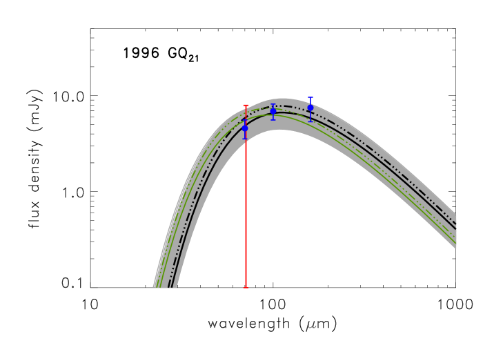
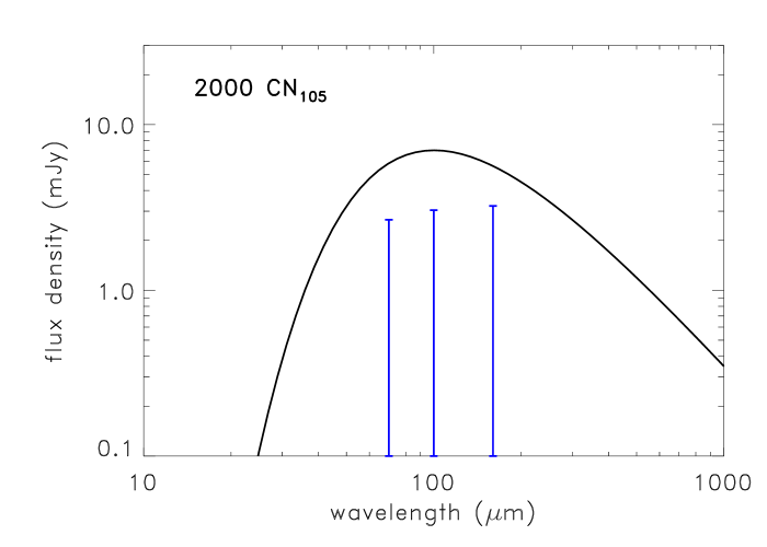
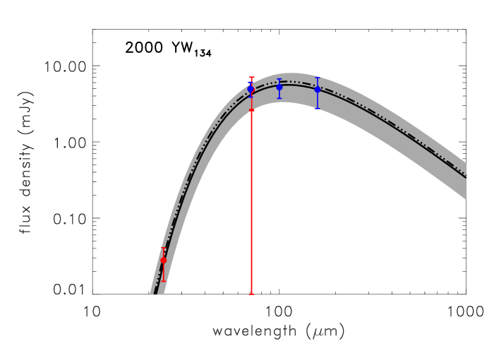
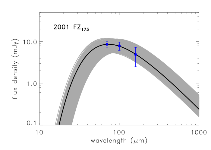
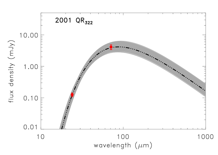
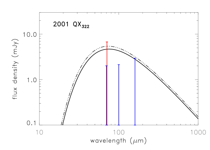
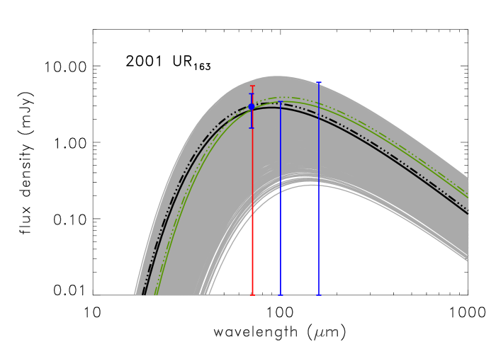
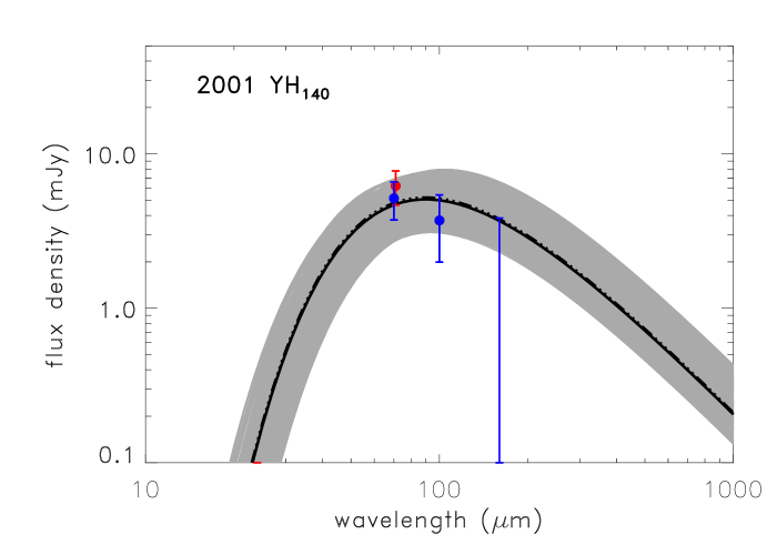
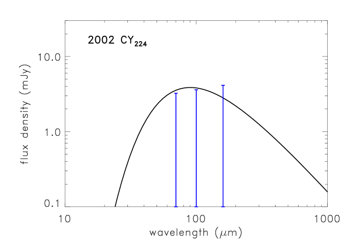
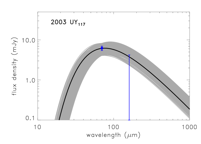
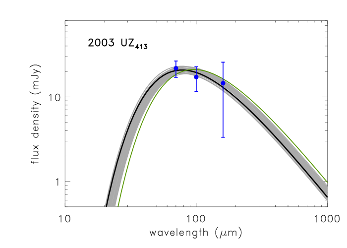
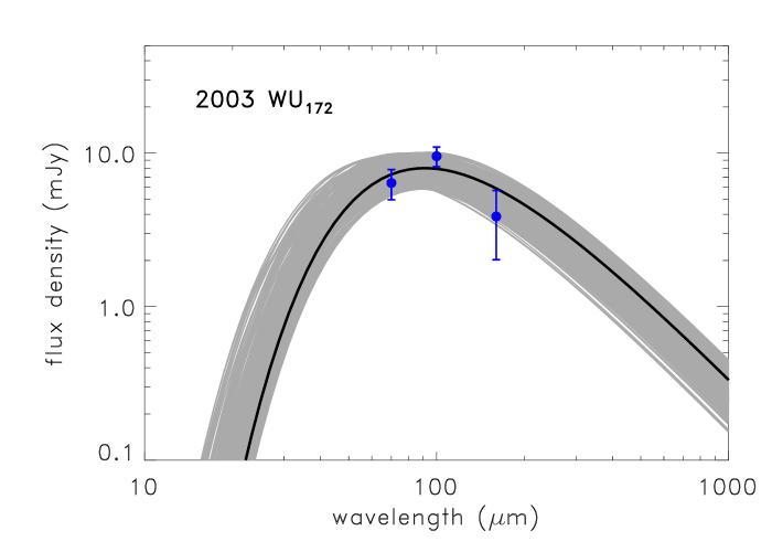
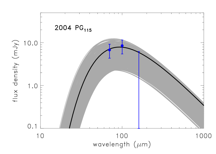
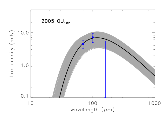
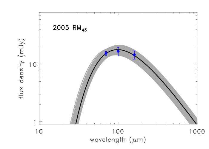
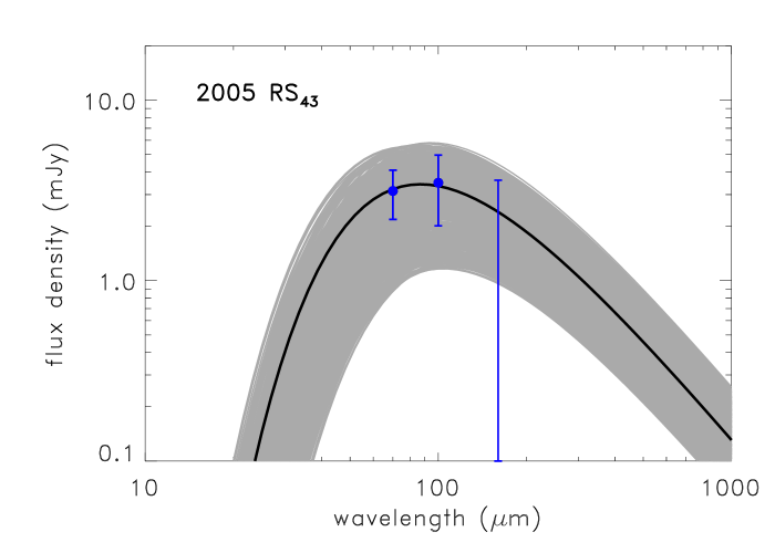
We derived new albedo, effective diameter, and beaming parameter values for 20 trans-Neptunian resonant and scattered disk objects via NEATM radiometric modeling using mainly Herschel/PACS data, in some cases supplemented by Spitzer/MIPS measurements, and for 3 targets based solely on Spitzer/MIPS data. The results are presented in Table 4, and the best-fit radiometric model fits are shown in Figs. 2 and 3. Due to non-detections (upper limits) of the thermal emission at all bands in the case of 2002 CY₂₂₄ we were only able to derive an upper limit for the effective diameter and a lower limit for the geometric albedo.

Figure 1: Beaming parameter vs. the heliocentric distance of the target at the time of the observation. Red symbols indicate the targets from the present paper for which the beaming parameter could be derived within the predefined limits. Gray symbols in the background indicate the beaming parameters from Lellouch et al. (2013).

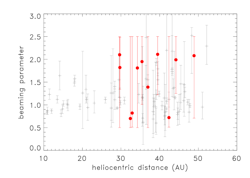
The fitted beaming parameters of those targets for which we did not use fixed-$\eta$ are plotted in Fig. 1 as a function of the heliocentric distance (red symbols). Compared with the Lellouch et al. (2013) beaming parameters (gray symbols in Fig. 1), in general the new targets present higher $\eta$ values, with a mean value of $\eta$ = 1.56 and standard deviation of d$\eta$ = 0.53, while this is 1.18 for the Lellouch et al. (2013) objects. A sample compiled from the Lellouch et al. (2013) targets with heliocentric distances of r_h $\geq$ 29 AU and from our floating-$\eta$ fit targets gives an average beaming parameter of $\eta$ = 1.25, and we used this value for the fixed-$\eta$ radiometric fitting (see Sect. 2.3).

It should be noted that objects presented in this paper are among the faintest ones in the “TNOs are Cool” sample. This is reflected in the large flux density uncertainties, and also in the radiometric modeling in the large $\eta$ uncertainties for many objects; in these cases the observed fluxes could be fitted with a large range of beaming parameters, as also shown in Figs. 2 and 3.

Table 4: Radiometric fit results of our new targets. Column headings are (from left to right) object name; Data: P:PACS, M:MIPS; Diam: diameter of object; p_V: geometric albedo; $\eta$: beaming parameter; *: fixed $\eta$ was used.

Object	Data	Diam (km)	Pv	$\eta$
(32929) 1995 QY9	M	$<210$	$>0.022$	$1.25^{*}\pm 0.35$
(26181) 1996 GQ21	P/M	$456^{+89}_{-105}$	$0.060^{+0.040}_{-0.022}$	$2.41^{+0.09}_{-1.40}$
	P/M	$352^{+46}_{-61}$	$0.098^{+0.046}_{-0.030}$	$1.25^{*}\pm 0.35$
(40314) 1999 KR16	P	$202^{+108}_{-36}$	$0.307^{+0.156}_{-0.178}$	$0.53^{+1.84}_{-0.02}$
	P	$271^{+39}_{-45}$	$0.177^{+0.076}_{-0.048}$	$1.25^{*}\pm 0.35$
(523588) 2000 CN105	P	$<440$	$>0.044$	$1.25^{*}\pm 0.35$
(82075) 2000 YW134	P/M	$437^{+118}_{-137}$	$0.133^{+0.173}_{-0.051}$	$1.99^{+0.51}_{-0.74}$
(82155) 2001 FZ173	P	$212^{+157}_{42}$	$0.121^{+0.065}_{-0.082}$	$0.70^{+1.80}_{-0.20}$
(139775) 2001 QG298	P	$<215$	$>0.070$	$1.25^{*}\pm 0.35$
2001 QR322	M	$178^{+61}_{-37}$	$0.033^{+0.021}_{-0.015}$	$1.82^{+0.66}_{-0.48}$
2001 QX322	P/M	$<210$	$>0.080$	$1.25^{*}\pm 0.35$
(42301) 2001 UR163	P/M	$261^{+209}_{-91}$	$0.427^{+0.624}_{-0.297}$	$0.59^{+1.9}_{-0.09}$
	P/M	$367^{+103}_{-197}$	$0.220^{+0.832}_{-0.090}$	$1.25^{*}\pm 0.35$
(126154) 2001 YH140	P/M	$252^{+148}_{-52}$	$0.143^{+0.144}_{-0.094}$	$1.24^{+1.26}_{-0.62}$
(119878) 2002 CY224	P	$<220$	$>0.098$	$1.25^{*}\pm 0.35$
2002 GP32	P	$234^{+47}_{-84}$	$0.063^{+0.105}_{-0.026}$	$2.47^{+0.03}_{-1.90}$
	P	$181^{+37}_{-47}$	$0.096^{+0.105}_{-0.040}$	$1.25^{*}\pm 0.35$
(133067) 2003 FB128	P	$218^{+91}_{-108}$	$0.047^{+0.144}_{-0.025}$	$1.81^{+0.69}_{-1.31}$
(469505) 2003 FE128	P	$137^{+123}_{-37}$	$0.184^{+0.160}_{-0.145}$	$0.51^{+1.99}_{-0.01}$
	P	$189^{+71}_{-89}$	$0.079^{+0.266}_{-0.040}$	$1.25^{*}\pm 0.35$
2003 QX111	M	$293^{106}_{-93}$	$0.033^{+0.164}_{-0.025}$	$2.11^{+0.39}_{-0.89}$
(143707) 2003 UY117	P	$196^{+114}_{-54}$	$0.182^{+0.195}_{-0.103}$	$0.82^{+1.68}_{-0.31}$
(455502) 2003 UZ413	P	$472^{+122}_{-25}$	$0.151^{+0.025}_{-0.064}$	$0.53^{+0.42}_{-0.03}$
	P	$650^{+1}_{-175}$	$0.075^{+0.076}_{-0.006}$	$1.25^{*}\pm 0.35$
(450265) 2003 WU172	P	$261^{+48}_{-114}$	$0.074^{+0.171}_{-0.050}$	$2.10^{+0.40}_{-1.60}$
(307982) 2004 PG115	P	$334^{+1}_{-191}$	$0.101^{+0.534}_{-0.005}$	$1.39^{+1.11}_{-0.89}$
(303775) 2005 QU182	P	$584^{+155}_{-144}$	$0.129^{+0.115}_{-0.046}$	$2.08^{+0.42}_{-1.37}$
(145451) 2005 RM43	P	$524^{+96}_{-103}$	$0.102^{+0.057}_{-0.029}$	$1.95^{+0.55}_{-0.94}$
(308379) 2005 RS43	P	$228^{+112}_{-58}$	$0.311^{+0.247}_{-0.182}$	$0.72^{+1.78}_{-0.21}$

Figure 2: NEATM fits of the thermal emission of our target sample. Black solid and dash-dotted curves represent the spectral energy distribution of the best-fit (lowest $\chi^{2}$) model for the epochs of the PACS and MIPS measurements, respectively. The gray area shows the zone of NEATM model curves that are compatible with the observed measurement uncertainties. In those cases when the floating $\eta$ fits converged to one of the beaming parameter limits, the fit was repeated with a fixed beaming parameter of $\eta$ = 1.25, represented by the green curves (not in all panels). Red and blue symbols represent the measured MIPS and PACS flux densities, respectively, color-corrected according to the best-fit NEATM model, at their respective epochs. In those cases when only flux density upper limits were available, we show the SED of the NEATM model with the diameter and geometric albedo limits presented in Table 4.

Figure 3: Continuation of Fig. 2

3.2 Individual targets

The NEATM-fits of the individual targets are presented in Fig. 2.

(82075) 2000 YW₁₃₄

was observed in the Science Verification Phase of the Herschel Space Observatory with the PACS photometer, in chop-nod mode (Müller et al., 2010). Those measurements provided only upper limits of F₇₀ $\leq$ 5 mJy and F₁₆₀ $\leq$ 8 mJy in the 70 and 160 $\mu$m bands, setting upper limits on the effective diameter, D_eff $\leq$ 500 km, and a lower limit of $p_{\mathrm{V}}$ $\geq$ 0.08 on the geometric albedo. These limits are in agreement with our newly derived, system-integrated values of D_eff = 437${}^{+118}_{-137}$ km and $p_{\mathrm{V}}$ = 0.13${}^{+0.17}_{-0.05}$. 2000 YW₁₃₄ is a binary, with a brightness difference of $\Delta m$ = 1$\aas@@fstack{m}$3 between the two components (Stephens & Noll, 2006). This provides effective diameters of D_eff = 382 km and 210 km, assuming equal albedos for the primary and secondary.

(139775) 2001 QG₂₉₈

is a plutino showing a large amplitude light curve, suggesting that it is a contact binary system (Lacerda & Jewitt, 2007). Due to the non-detections (upper limits) in all PACS bands, we were only able to derive an upper limit for the equivalent diameter D_eff $<$ 215 km for the system and a lower limit for the geometric albedo, $p_{\mathrm{V}}$ $>$ 0.07. Lacerda & Jewitt (2007) and Lacerda (2011) obtained a solution for the system from multi-epoch visible light curve observations that the density of the system (for both components) is $\rho$ = 0.59 g cm^-3 with a secondary-to-primary mass ratio of q = 0.84, and two triaxial ellipsoids with primary-to-secondary axis ratios of B/A = 0.72, C/A = 0.64, b/a =0.45 and c/a = 0.41, using a Roche model (lowest $\chi^{2}$ model with lunar-type scattering). Assuming that the two bodies have equal albedos and that the Herschel measurements represent a mean rotational and orbital phase configuration in terms of apparent cross sections of the components, the semi-axes of the ellipsoids are A = 115 km, B = 82 km, C = 72 km, a = 146 km, b = 66 km, and c = 60 km, using the upper limit of D_eff $<$ 215 km, from our radiometric solution.

2001 QR₃₂₂

is the first Neptune Trojan discovered, and it may have a dynamically unstable orbit (Horner & Lykawka, 2010). Our measurements suggest a very dark surface ($p_{\mathrm{V}}$ = 0.03$\pm 0.02$) and an effective diameter of D_eff = 178${}^{+61}_{-37}$ km.

(42301) 2001 UR₁₆₃

is one of the reddest objects known in the Solar System (B–R = 2.05$\pm$0.10 Santos-Sanz et al., 2009). Our floating beaming parameter fit converges to a very low value of $\eta$ = 0.5, the lowest limit in our calculations. These extremely low beaming parameters would be expected for a rough surface and low thermal parameters (Spencer et al., 1989; Spencer, 1990). The corresponding albedo and diameter would be D_eff = 261${}_{-91}^{+209}$ km and $p_{\mathrm{V}}$ = 0.43${}_{-0.30}^{+0.62}$. We have repeated this calculation by applying a fixed beaming parameter of $\eta$ = 1.25, as in previous “TNOs are Cool” sample papers (e.g., Santos-Sanz et al. 2012). This provides a size of D_eff = 367${}_{-197}^{+103}$ km and a geometric albedo of $p_{\mathrm{V}}$ = 0.22${}_{-0.09}^{+0.83}$.

(126154) 2001 YH₁₄₀

was also observed in the Science Verification Phase (SVP) of the Herschel Space Observatory with the PACS photometer, in chop-nod mode (Müller et al., 2010) in two bands, 70 and 160 $\mu$m. The monochromatic flux densities obtained are F${}_{70}^{\prime}$ = 9.8$\pm$2.9 mJy and F${}_{160}^{\prime}$ $\leq$ 13 mJy (i.e., an upper limit in the latter case). The in-band flux densities derived in our present work, F₇₀ = 5.08$\pm$ 1.40 mJy and F₁₀₀= 3.67$\pm$ 1.70 mJy, are notably lower then suggested by the earlier measurements, and we provide a more strict upper limit of F₁₆₀ $\leq$ 1.95 mJy (1$\sigma$). The high flux densities obtained in the SVP measurements may be a consequence of the weak reliability of the chop-nod observing mode that was superseded by the scan-map mode in the later phases of the Herschel mission (Nielbock et al., 2013), and are not necessarily true flux density changes between the two observational epochs. Based on our new radiometric fits 2001 YH₁₄₀ is smaller and brighter, D_eff = 252${}_{-52}^{+148}$ km and $p_{\mathrm{V}}$ = 0.14${}_{-0.09}^{+0.14}$, than that derived from the Herschel SVP measurements (D $\approx$ 350 km and $p_{\mathrm{V}}$ $\approx$ 0.08).

2003 UZ₄₁₃

is a plutino with a rotation period of P = 4.13$\pm$0.05 h and a light curve amplitude of $\Delta m$ = 0.13$\pm$0.03 mag (Perna et al., 2009). The observed fast rotation and the light curve amplitude might be compatible with a Jacobi ellipsoid with $a$/$b$ $\approx$ 1.13; however, this would require a high density of $\rho$ = 2.3–3.0 g cm^-3, a peculiarly high value among trans-Neptunian objects. For 2003 UZ₄₁₃, the floating $\eta$ NEATM fit in our radiometric analysis cannot provide a well-defined solution ($\eta$ converges to the minimum allowed value of 0.5). By applying a fixed beaming parameter of $\eta$ = 1.25, we derived an effective diameter of D_eff = 650${}^{+1}_{-175}$ km and a geometric albedo of $p_{\mathrm{V}}$ = 0.08${}^{+0.08}_{0.01}$.

(145451) 2005 RM₄₃

is a detached object that was also observed by Perna et al. (2009), who obtained a rotation period of P = 9.00$\pm$0.06 h and a light curve amplitude of $\Delta m$ = 0.12$\pm$0.05 mag. A Jacobi ellipsoid model provides a density estimate of $\rho$ $\approx$ 0.55g cm^-3. According to our radiometric fit, the diameter is D_eff = 524${}_{-103}^{+96}$ km with a geometric albedo of $p_{\mathrm{V}}$ = 0.10${}^{+0.06}_{-0.03}$.

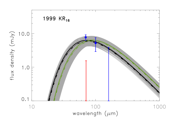
(40314) 1999 KR₁₆ and 2005 QU₁₈₂

were analyzed previously in Santos-Sanz et al. (2012), but the Herschel/PACS 100 $\mu$m data were inconsistent (too low) with the flux densities obtained in the 70 and 160 $\mu$m bands, and we therefore reanalyzed these measurements in the present work.

As discussed in Sect. 2.1, in our reduction we used double-differential images instead of supersky-subtracted images, as in Santos-Sanz et al. (2012), to minimize the effect of nearby background sources. In the case of 1999 KR₁₆ Vilenius et al. (2018) reanalyzed the PACS measurements and found that there was a bright background source near the target at one of the epochs; due to this contamination they decided not to use the visit 2 measurements (i.e., their photometry is based on a single-epoch measurement, strongly affected by the background).

For 1999 KR₁₆ Santos-Sanz et al. (2012) obtained the monochromatic flux densities of F${}_{70}^{\prime}$ = 5.7$\pm$0.7 mJy, F${}_{100}^{\prime}$ = 3.5$\pm$1.0 mJy, and F${}_{160}^{\prime}$ = 4.6$\pm$2.2 mJy. Our in-band flux densities are F₇₀ = 7.61$\pm$1.44 mJy, F₁₀₀ = 5.21$\pm$2.29 mJy, and F₁₆₀ $<$ 1.98 mJy. The fixed beaming parameter fit of $\eta$ = 1.2 in Santos-Sanz et al. (2012) provided D_eff = 254$\pm$37 km and $p_{\mathrm{V}}$ = 0.20${}^{+0.07}_{-0.05}$. This is similar to our floating $\eta$ fit, D_eff = 202${}^{+108}_{-36}$ km and $p_{\mathrm{V}}$ = 0.31${}^{+0.16}_{-0.18}$. However, in this latter case the best-fit beaming parameter is $\eta$ = 0.53${}^{+1.84}_{-0.02}$, an extremely low value. For 2005 QU₁₈₂ Santos-Sanz et al. (2012) obtained F${}_{70}^{\prime}$ = 4.5$\pm$0.9 mJy, F${}_{100}^{\prime}$ = 2.5$\pm$1.1 mJy, and F${}_{160}^{\prime}$ = 8.4$\pm$3.0 mJy, providing D_eff = 416$\pm$73 km and $p_{\mathrm{V}}$ = 0.33${}^{+0.16}_{-0.11}$ using a fixed $\eta$ = 1.2 fit. In our photometry using the double-differential products, the monochromatic flux densities are F₇₀ = 4.41$\pm$1.28 mJy, F₁₀₀ = 6.94$\pm$2.11 mJy, and F₁₆₀ $<$ 2.73 mJy, and the corresponding effective diameter and geometric albedo are D_eff = 584${}^{+155}_{-144}$ km and $p_{\mathrm{V}}$ = 0.13${}^{+0.12}_{-0.05}$, with a best-fit beaming parameter of $\eta$ = 2.08${}^{+0.42}_{-1.37}$ (i.e., a notably larger size and lower albedo).

Figure 4: Albedo vs. visible color, quantified by the spectral slope $S^{\prime}$. Upper panel: TNOs from Lacerda et al. (2014) using updated albedo and spectral slope values in some specific cases. The three clusters identified are indicated in blue, red, and green. Ellipses (distorted due to the logarithmic $p_{\mathrm{V}}$ scale) with crosshairs indicating the centers and variance values of the clusters in the albedo–spectral slope plane. Objects indicated by black symbols have ambiguous identifications. Middle panel: Same as the top panel (TNOs from Lacerda et al., 2014), but with the new objects of the present paper overplotted. The following symbols were used: $\triangledown$ – plutinos; $\boxtimes$ – detached objects; $\times$ – scattered disk objects; $\Diamond$ – outer resonants; $\Circle$ – inner resonants; $\star$ – middle resonants; $\Box$ – 1999 CD₁₅₈ (Vilenius et al., 2018); $\otimes$ – 1996 TO₆₆ (Vilenius et al., 2018). Bottom panel: Clusters in the albedo vs. spectral slope plot using all 120 objects, including those from Lacerda et al. (2014) and the new targets from the present paper.

4 Discussion

4.1 Thermal intertia estimates

Lellouch et al. (2013) estimated thermal inertia from the $\eta$ values derived and obtained a decrease in $\Gamma$ from $\sim$5 $\mathrm{J}\,m^{-2}\,s^{-1/2}K^{-1}$to $\sim$2 $\mathrm{J}\,m^{-2}\,s^{-1/2}K^{-1}$  from $\sim$25 AU to heliocentric distances beyond 40 AU. Following a similar approach we also estimated the thermal inertia values for our targets. The phase integral $q$ was calculated applying both the standard Bowell et al. (1989) formula with a G = 0.15 slope parameter, and also using the geometric albedo dependent formula by Brucker et al. (2009). These two methods resulted in subsolar temperatures with negligible differences (typically $\lesssim$1 K, the largest difference is $\sim$4 K for the high albedo target 2002 CY₂₂₄) and with a negligible effect on the final results. We assumed a uniform P = 8 h rotation period for all targets. We used two subsolar latitudes, $\beta_{ss}$ = 32.7° (average values of random orientation spin axis directions) and also $\beta_{ss}$ = 0°, as some specific (high, $\eta$ $\geq$ 2.0) beaming parameter values could not be reproduced with $\beta_{ss}$ = 32.7°. We allowed a roughness from $s$ = 0 to 60° (zero to high roughness). The thermal inertias obtained were similar in the two $\beta_{ss}$ cases for a specific target, but showed a wide range of possible values, partly due to the typically large uncertainties in the $\eta$ determination, and the ambiguity that different combinations of $\Theta$, $\beta_{ss}$, and $s$ can result in the same beaming parameter at the end. The median values for our sample were 1.9 $\mathrm{J}\,m^{-2}\,s^{-1/2}K^{-1}$  for $\beta_{ss}$ = 0° and 3.1 $\mathrm{J}\,m^{-2}\,s^{-1/2}K^{-1}$  for $\beta_{ss}$ = 32.7°; for the same target (albedo and heliocentric distance) a higher $\beta_{ss}$ value results in a higher $\Gamma$, as a higher $\Theta$ is needed to obtain the same beaming parameter (see fig. 4 in Lellouch et al., 2013). These thermal inertias are compatible with those obtained by Lellouch et al. (2013) for the same heliocentric distance range.

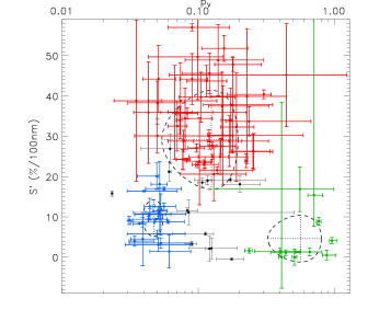
4.2 Albedo-color diagram

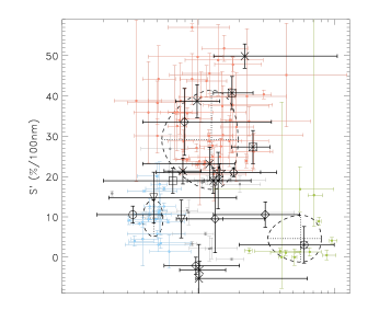
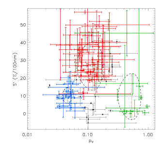
As was demonstrated in Lacerda et al. (2014) objects in the trans-Neptunian region can be divided into two main clusters based on their geometric albedo and visible color properties. We repeated this analysis using the mclust package in R (Fraley et al., 2018).

We used two main datasets. The first is the Lacerda et al. (2014) sample using mainly the geometric albedo and spectral slope data derived from the original papers, but using new albedo and color values in the cases when they were updated according to the latest reduction of the Herschel and Spitzer data – e.g., 2007 OR₁₀ (Pál et al., 2016) and 2007 UK₁₂₆ (Schindler et al., 2017) – or by new occultation measurements (Haumea, Ortiz et al., 2017; Müller et al., 2018b). New targets given in the present paper are not included in this dataset.

The second dataset contains all objects, i.e., the Lacerda et al. (2014) sample and also our new targets, and two additional targets, 1996 TO₆₆ and 1999 CD₁₅₈ from (Vilenius et al., 2018). 1996 TO₆₆ is considered to be a Haumea collisional family member, while 1999 CD₁₅₈ is thought to be dynamical interloper with this family. We also considered the relatively wide ranges obtained for the albedos and colors from the disk-resolved measurements of Pluto and Charon (Grundy et al., 2016) when drawing their data points in the corresponding figures.

In both cases we run the MClust package for a multiple number of cluster components assumed and also using different data models. The results are presented in Fig. 4 and summarized in Table 5. In the case of the first dataset (Lacerda et al., 2014 sample) the smallest residuals were obtained using an ellipsoidal, varying volume and shape data model (VVI) with three groups. These clusters are very closely identical with the clusters obtained by Lacerda et al. (2014), i.e., we can identify a dark-neutral group (DN, blue symbols in Fig. 4) and a bright-red group (BR, red symbols), and a third group at high albedos and nearly solar colors. This last group is not defined explicitly by Lacerda et al. (2014) as the related objects are essentially excluded from that analysis; these objects are the brightest dwarf planets (Pluto, Eris, Makemake) and the members of the Haumea collisional family. As we left these objects in the dataset, a third, “bright-neutral” (BN) group could be identified (Fig. 4, left panel, green symbols). We note that the objects with uncertain cluster identification are indicated by black symbols in the figure (located typically between two clusters).

We plotted the new targets over the clusters of the original sample in the middle panel of Fig. 4. These targets extend the spectral slope range to smaller values (close to solar) even in the p_V $>$ 0.1 region, where there were few objects in the original sample. Including the new targets in the cluster modeling results in somewhat different clusters (Fig. 4, right panel), but the main structure (the number, location, and extension of the groups) remains basically unchanged (see Table 5). The groups we identified both in the original and in the full sample match the clusters identified by Lacerda et al. (2014) very closely.

While most of our new objects follow the previously identified main groups, there is an important new feature. In the Lacerda et al. (2014) analysis the albedo–color range of 0.10 $\lesssim$ $p_{\mathrm{V}}$ $\lesssim$0.40 and 5 $\lesssim$ $S^{\prime}$ $\lesssim$15  [%/100 nm] remained empty, in our sample we have three objects, 2000 YW₁₃₄, 1995 QY₉, and 2005 RS₄₃ that fall here. While many inner Solar System objects have surfaces matching the albedos and colors of our dark and neutral group (Lacerda et al., 2014), objects with these moderate albedos and slightly red colors cannot be found even in the inner Solar System beyond the 5:3 resonance with Jupiter (including Hildas and Jupiter Trojans), only at heliocentric distances of $\lesssim$3.5 au (DeMeo & Carry, 2014). These objects seem to lack the red material that is common among most trans-Neptunian objects in this albedo range. We note that the Neptune irregular satellite Nereid has albedo and color similar to those of these objects (Kiss et al., 2016). Targets with nearly solar colors and medium albedos (0.08 $\lesssim$ $p_{\mathrm{V}}$ $\lesssim$ 0.30) all have ambiguous identifications in this clustering scheme.

Lacerda et al. (2014)			Original sample			All targets
Mathematica/FindClusters			R/MClust, VVI			R/MClust, VVI
pV	$S^{\prime}$	ID	pV	$S^{\prime}$	ID	pV	$S^{\prime}$	ID
$\sim$0.05	$\sim$10	DN	0.047$\pm$0.008	9.7$\pm$4.6	DN	0.046$\pm$0.008	10.0$\pm$4.5	DN
$\sim$0.15	$\sim$35	BR	0.125$\pm$0.071	29.1$\pm$12.3	BR	0.121$\pm$0.056	26.7$\pm$13.6	BR
$>$0.30	$\sim$0	BN	0.564$\pm$0.239	4.6$\pm$5.8	BN	0.538$\pm$0.221	9.5$\pm$13.0	BN

Table 5: Clusters identified by Lacerda et al. (2014, Col. 1), using the Lacerda et al. (2014) sample with updates (this work, Col. 2), and using all targets (this work, Col. 3). Clusters are characterized here by their mean geometric albedo (p_V) and spectral slope ($S^{\prime}$, %/1000 $\AA$), and the standard deviations using an ellipsoidal varying volume and shape data model. In the second row we also list the tools used to identify the clusters.

Figure 5: Spectral slope vs. geometric albedo for resonant (left), and scattered disk and detached objects (right). Regions delineated with dashed and dash-dotted lines correspond to the 1 $\sigma$ contours of the clusters identified in our analysis using the original and full samples, respectively. Filled circles and stars mark plutinos (3:2 resonance) and other resonant objects, respectively, in the left panel. Filled squares and triangles indicate scattered disk and detached objects in the right panel. Black symbols indicate objects with ambiguous cluster assignments.

We also found that the objects 2004 PG₁₁₅ and 2005 RM₄₃, although they are likely associated with the DN group, are located so far from the group center with their negative spectral slopes and $p_{\mathrm{V}}$ $\approx$ 0.10 albedos that their group assignment can be considered ambiguous. Lacerda et al. (2014) found that objects in relic populations, i.e., those that formed and remained in the outer Solar System (cold classical KBOs and objects in the outer resonances), possess exclusively bright red surfaces, while populations with dynamically more complex origin (Centaurs, scattered disk objects, hot classical KBOs, plutinos) show mixed surfaces. Our new targets follow this general picture; for example, new scattered disk objects can be found both in the DN and the BR groups, while detached objects and targets from the outer resonances can exclusively be found among BR objects.

4.3 Impact on size distributions

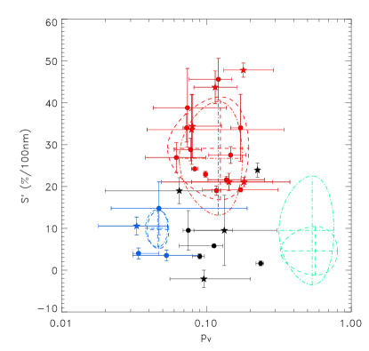
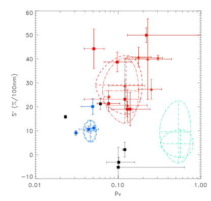
Size distribution is an essential characteristic of small body populations, providing information on the collisional history. As diameters of small bodies cannot be obtained directly in most cases, it is difficult to obtain a reliable size distribution. Usually it is necessary to rely on the absolute magnitude distribution that can be derived directly from the observations of these objects (Gladman et al., 2001). Typically, a single, mean albedo value known from other measurements can be used (e.g., radiometry or occultations) to convert between the diameter and the absolute magnitude in the corresponding distributions. Mommert et al. (2012), among others, used an average albedo of 0.08$\pm$0.03 to convert from absolute magnitude to effective diameter and to derive the size distribution of plutinos. However, as we have shown above, trans-Neptunian populations, including scattered disk and resonant objects show a bimodal albedo and color distribution; therefore, the application of a bimodal albedo (e.g., using the color as a proxy for the mean albedo) might be more appropriate.

In Fig. 5 we drew the plutinos, objects in other (not 3:2) resonances, and scattered disk and detached objects over the main groups identified by our cluster analysis. Bimodal and color-dependent albedo is clearly the case for scattered disk and detached objects (right panel). Here the objects in the specific groups, $p_{\mathrm{V}}$(SDO,DN) = 0.044$\pm$0.008 and $p_{\mathrm{V}}$(SDO,BR) = 0.119$\pm$0.054, follow the general albedos of the larger samples (Table 5). We note that there is no detached object in the DN group. The three objects with very low spectral slope values ($S^{\prime}$ $\lesssim$ 0, 2000 YW₁₃₄, 1995 QY₉ and 2005 RS₄₃) seem to have albedos similar to the BR group, $p_{\mathrm{V}}$ $\approx$ 0.12. The case is different for the resonant objects, including the plutinos, due to the presence of several new objects in the range 0.10 $\lesssim$ $p_{\mathrm{V}}$ $\lesssim$0.40 and 5 $\lesssim$ $S^{\prime}$ $\lesssim$15  [%/100 nm] (see the discussion above), making the color-to-albedo assignment ambiguous. It is, however, still the case for the BR group that their colors correspond to a relatively well-defined albedo, $p_{\mathrm{V}}$(RTNO,BR) = 0.12$\pm$0.04.

Figure 6: Geometric albedo ($p_{\mathrm{V}}$) vs. diameter (D) for the full scattered disk and resonant sample. The clusters are color-coded: blue – DN; red – BR; green – BN; gray – ambiguous group assignment. Filled circles, stars, squares, and triangles indicate plutinos, other resonances, scattered disk objects, and detached objects, respectively. Open circles are any other dynamical class, except the Centaurs that are shown as asterisks. Dotted lines represent the constant absolute magnitudes, as labeled. Purple symbols with dashed lines indicate those targets for which only diameter upper- and albedo lower limits could be derived in this paper.

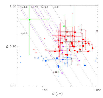
It is also an important question whether objects with different sizes have the same typical albedos, and whether the same mean albedo (or albedo distribution) can be used to convert from absolute magnitudes to effective diameters within the same albedo-color group. In Fig. 6 we plot the geometric albedos of resonant and scattered disk objects versus the effective diameter derived form radiometric data. We have to emphasis that this sample is not unbiased, as objects in the “TNOs are Cool” studies (where the majority of these data are from) were selected to cover different dynamic classes, sizes, or absolute magnitude ranges, and should have been foreseen to be detectable by the Herschel Space Observatory, assuming a uniform 8% geometric albedo (Müller et al., 2009; Kiss et al., 2014). In the present sample no obvious trend is visible within any of the albedo-color groups. There is a general trend, considering all objects together, that smaller objects are darker, but this is dominated by the presence of Centaurs (asterisks in Fig. 6) that are found at smaller heliocentric distances and remain observable above $H_{\mathrm{V}}$ $\lesssim$ 9.0, which is an absolute limit for the targets in the other dynamical families. In addition, darker objects are observable at smaller sizes in thermal emission at the same heliocentric distance, and that was the main criterion when the “TNOs are Cool” object list was compiled. This indicates that to our present knowledge a color-dependent and dynamical class-dependent albedo is probably suitable to transform between absolute magnitude and size distributions, as discussed above.

5 Summary

We determined the size and albedo of 23 trans-Neptunian resonant and scattered disk objects using data mainly based on the “TNOs are Cool” Herschel Open Time Key Programme observations, supplemented in some cases by Spitzer Space Telescope data. Together with the previous studies based on the “TNOs are Cool” data, this is the largest reliable set of size and albedo estimates for objects in the outer resonances in the Kuiper belt. We confirm the results of a previous investigation (Lacerda et al., 2014) that trans-Neptunian objects can be divided into albedo-color groups and that objects in relic populations exclusively have bright-red surfaces, strengthening the evidence for a compositional discontinuity in the young Solar System. We suggest that size distribution studies based on absolute magnitude distributions use the bimodal albedos, specific for the dark-neutral and bright-red groups in all dynamical populations, for example using colors or spectral slopes as a proxy for albedo-color group membership (e.g., Ayala-Loera et al., 2018).

References

- Aaron et al. (2009) Aaron, F.D., Alexa, C., Anrdeev, V., et al. (the ’H1 collaboration’), 2009, Eur. Phys. J. C, 63, 625
- Ali-Lagoa et al. (2018) Ali-Lagoa, V., Müller, T.G., Usui, F., Hasegawa, S., 2018, A&A, 612, A85
- Alvarez-Candal et al. (2011) Alvarez-Candal, A., Pinilla-Alonso, N., Licandro, J., et al., 2011, A&A, 532, A130
- Ayala-Loera et al. (2018) Ayala-Loera, C., Alvarez-Candal, A., Ortiz, J.L., et al., 2018, MNRAS, 481, 1848
- Bannister et al. (2018) Bannister, M.T., Gladman, B.J., Kavelaars, J.J., et al., 2018, ApJS, 236, 18
- Barucci and Doressoundiram (1999) Barucci, M.A., and Doressoundiram, A., 1999, Icarus, 142, 476
- Boehnhardt et al. (2014) Boehnhardt, H., Schulz, D., Protopapa, S., Götz, C., 2014,EM&P, 114, 35
- Bowell et al. (1989) Bowell, E.G., Hapke, B., Domingue, D., Lumme, K., Peltoniemi, J., Harris, A.W., 1989. Application of photometric models to asteroids. In: Gehrels, T., Matthews, M.T., Binzel, R.P. (Eds.), Asteroids II. University of Arizona Press, pp. 524–555.
- Brown & Butler (2017) Brown, M.E., Butler, B.J., 2018, AJ, 156, 164
- Brucker et al. (2009) Brucker, M.J., Grundy, W.M., Stansberry, J.A., et al., 2009, Icarus, 201, 284
- Buie et al. (2003) Buie, M.W., Jordan, A.B., Wasserman, L.H., et al., 2003, MPEC 2003-H07
- Delbo et al. (2003) Delbo, M., Harris, A.W., Binzel, R.P., Pravec, P., Davies, J.K., 2003, Icarus, 266, 116
- Delbo et al. (2015) Delbo, M., Mueller, M., Emery, J. P., Rozitis, B., & Capria, M. T. 2015, Asteroid Thermophysical Modeling, in: Asteroids IV., ed. P. Michel, F. E. DeMeo, & W. F. Bottke, 107–128
- DeMeo et al. (2009) DeMeo, F.E., Fornasier, S., Barucci, M.A., 2009, A&A, 493, 283
- DeMeo & Carry (2014) DeMeo, F.E. & Carry, B., 2014, Nature, 505, 629
- Doressoundiram et al. (2002) Doressoundiram, A., Peixinho, N., de Bergh, C. et al., 2002, AJ, 124, 2279
- Doressoundiram et al. (2005) Doressoundiram, A., Peixinho, N., Doucet, C., et al., 2005, Icarus, 174, 90
- Doressoundiram et al. (2007) Doressoundiram, A., Peixinho, N., Moullet, A., et al., 2007, AJ, 134, 2186
- Duffard et al. (2014) Duffard, R., Pinilla-Alonso, N., Santos-Sanz, P., 2014, A&A, 564, A92
- Engelbracht et al. (2007) Engelbracht, C.W., Blaylock, M., Su, K.Y.L., 2007, PASP, 119, 994
- Farkas-Takács et al. (2017) Farkas-Takács, A.I., Kiss, Cs., Pál, A., et al., 2017, AJ, 154, 119
- Fornasier et al. (2013) Fornasier, S., Lellouch, E., Müller, T.G., et al. 2013, A&A, 555, A15
- Fraley et al. (2018) Fraley, C., et al., 2018, Package ’mclust’, version Novermber 17, 2018
- Fraser et al. (2010) Fraser, W.C., Brown, M.E., Schwamb, M.E., 2010, Icarus, 210, 944
- Fraser et al. (2014) Fraser, W.C., Brown, M.E., Morbidelli, A., Parker, A., Batygin, K., 2014, ApJ, 782, 100
- Gladman et al. (2001) Gladman, B., Kavelaars, J. J., Petit, J.-M., et al., 2001, AJ, 122, 1051
- Gladman et al. (2012) Gladman, B., Lawler, S.M., Petit, J.-M. et al. 2012, AJ, 144, 23
- Gomes et al. (2008) Gomes, R. S., Fernández, J. A., Gallardo, T. et al. 2008, SSBN book, 259G
- Gordon et al. (2005) Gordon, K.D., Rieke, G.H., Engelbracht, C.W., et al. 2005, PASP, 117, 503
- Gordon et al. (2007) Gordon, K.D., Engelbracht, C.W., Fadda, D., et al. 2007, PASP, 119, 1019
- Grundy et al. (2016) Grundy, W.M., Binzel, R.P., Buratti, B.J., et al., 2016, Science, 351, 9189
- Hainaut & Delsanti (2002) Hainaut, O.R., & Delsanti, A.C., 2002, A&A, 389, 641
- Hainaut & Delsanti (2002) Hainaut, O.R. & Delsanti, A.C., 2002 A&A 389, 641
- Harris (1998) Harris, A.W. 1998, Icarus, 131, 291
- Herschel Science Center (2009) Herschel Science Centre, Herschel Products and Tools Contributor’s Guide, HERSCHEL-HSC-DOC-1405, 4 December 2009
- Horner & Lykawka (2010) Horner, J. & Lykawka, P.S., 2010, MNRAS, 405, 49
- Jurić et al. (2002) Jurić, M., Ivezić, Ž, Lupton, R.H., et al., 2002, AJ, 124, 1776
- Kiss et al. (2014) Kiss, Cs., Müller, Th.G., Vilenius, E., et al., 2014, ExA, 37, 161
- Kiss et al. (2016) Kiss, Cs., Pál, A., Farkas-Takács, A. I., et al., 2016, MNRAS, 457, 2908
- Kiss et al. (2016b) Kiss, Cs., Müller, T.G., 2016, User Provided Data Product upload of Herschel/PACS near-Earth asteroid observations, Release Note V 1.0, available at: http://archives.esac.esa.int/hsa/legacy/UPDP/COOLTNOs/tnosarecool.pdf
- Kiss et al. (2019) Kiss, Cs., Szakáts, R., Marton, G., et al., 2019, ’Small Bodies: Near and Far’ database of thermal infrared measurements of small Solar System bodies, Release Note: Public Release 1.2, 2019 March 29 (http://ird.konkoly.hu)
- Kiss et al. (2019b) Kiss, C., Marton, G., Parker, A.H., et al., 2019, Icarus, 334, 3
- Lacerda & Jewitt (2007) Lacerda P. & Jewitt, D.C., 2007, AJ, 133, 1393
- Lacerda (2011) Lacerda, P., 2011, AJ, 142, 90
- Lacerda et al. (2014) Lacerda, P., Fornasier, S., Lellouch, E., et al., 2014, ApJ, 793, L2
- Lellouch et al. (2013) Lellouch, E., Santos-Sanz P., Lacerda, P., et al., 2013, A&A 557, A60
- Lellouch et al. (2017) Lellouch, E., Moreno, R., Müller, T., et al., A&A 608, A45
- Lellouch et al. (2016) Lellouch, E., Santos-Sanz, P., Fornasier, S., et al., 2016, A&A 558, A2
- Mommert et al. (2012) Mommert, M., Harris, W., Kiss, Cs., et al., 2012, A&A 541, A93
- Mueller et al. (2012) Mueller, M., Stansberry, J., Mommert, M. & Grundy, W., 2012, ”TNO Diameters And Albedos: The Final MIPS Dataset”, AAS DPS meeting, #44, #310.13
- Müller et al. (2009) Müller, T.G., Lellouch, E., Böhnhardt, H., et al., 2009, EM&P, 105, 209
- Müller et al. (2010) Müller, T.G., Lellouch, E., Stansberry, J., et al., 2010, A&A, 518, L146
- Müller et al. (2011) Müller, T., Okumura, K., Klaas, U., 2011, PACS Photometer Passbands and Colour Correction Factors for Various Source SEDs, Herschel/PACS technical report, PICC-ME-TN-038
- Müller et al. (2018) Müller, T.G., Marciniak, A., Kiss, C., et al., 2018, Advances in Space Research, 62, 2326
- Müller et al. (2018b) Müller, T. G., Kiss, C., Ali-Lagoa, V. et al., 2018, Icarus, in press (arXiv:1811.09476)
- Müller et al. (2019) Müller, T., Lellouch, E., Fornasier, S., 2019, TNOs and Centaurs at thermal wavelengths, https://arxiv.org/abs/1905.07158
- Nielbock et al. (2013) Nielbock, M., Müller, Th.G., Klaas, U., et al., 2013, Experimental Astronomy, 36, 631
- Ortiz et al. (2017) Ortiz, J.L., Santos-Sanz, P., Sicardy, B., et al., 2017, Nature, 550, 219
- PACS Data Reduction Guide (2015) PACS Data Reduction Guide: Photometry, Issue user. Version 12, Nov. 2015
- PACS Observer’s Manual (2011) PACS Observer’s Manual, HERSCHEL-HSC-DOC-0832, Version 2.3, 08-June-2011
- Pál et al. (2012) Pál, A., Kiss, C., Müller, T.G., 2012, A&A 541, L6
- Pál et al. (2016) Pál, A., Kiss, C., Müller, T.G., 2016, AJ, 151, 117
- Perna et al. (2009) Perna, D., Dotto, E., Barucci, M. A., et al., 2009, A&A, 508, 451
- Perna et al. (2010) Perna, D., Barucci, M.A., Fornasier, S., et al., 2010, A&A, 510, A53
- Perna et al. (2013) Perna, D., Dotto, E., Barucci, M.A., et al., 2013, A&A, 554, A49
- Poglitsch et al. (2010) Poglitsch, A., Waelkens, C., Geis, N., et al., 2010, A&A, 518, L2
- Romanishin & Tegler (2005) Romanishin, W. & Tegler, S.C., 2005, Icarus, 179, 523
- Santos-Sanz et al. (2009) Santos-Sanz, P., Ortiz, J.L., Barrera, L., Boehnhardt, H., 2009, A&A, 494, 693
- Santos-Sanz et al. (2012) Santos-Sanz, P., Lellouch, E., Fornasier, S., 2012, A&A, 541, A92
- Schindler et al. (2017) Schindler, K., Wolf, J., Bardecker, J., et al., 2017, A&A, 600, A12
- Sheppard (2012) Sheppard, S.S., 2012, AJ, 144, 169
- Sheppard & Jewitt (2002) Sheppard, S.S., & Jewitt, D.C. 2002, AJ, 124, 1757
- Sheppard & Jewitt (2004) Sheppard, S.S. & Jewitt, D.C., 2004, AJ, 127, 3023
- Snodgrass et al. (2010) Snodgrass, C., Carry, B., Dumas, C., Hainaut, O., 2010, A&A 511, A72
- Spencer et al. (1989) Spencer, J.R., Lebofsky, L.A., Sykes, M.V., 1989, Icarus, 78, 337
- Spencer (1990) Spencer, J.R., 1990, Icarus, 83, 27
- Stansberry et al. (2007) Stansberry, J.A., Gordon, K.D., Bhattacharya, B., 2007, PASP, 119, 1038
- Stansberry et al. (2008) Stansberry, J., Grundy, W.M., Brown, M.E., et al., 2008, in The Solar System Beyond Neptune, Physical Properties of Kuiper Belt and Centaur Objects: Constraints from the Spitzer Space Telescope, p.161 (Tuscon, AZ: Univ. Arizona Press)
- Stansberry et al. (2012) Stansberry, J.A., Grundy, W.M., Mueller, M., et al., 2012, Icarus, 219, 676
- Stephens & Noll (2006) Stephens, D.C. & Noll, K.S., 2006, AJ, 131, 1142
- Szakáts et al. (2020) Szakáts, R., Müller, T., Ali-Lagoa, V., et al., 2020, A&A, 635, A54
- Vilenius et al. (2012) Vilenius, E., Kiss, C., Mommert, M. et al., 2012, A&A 541, A94
- Vilenius et al. (2014) Vilenius, E., Kiss, C., Müller, T., 2014, A&A 564, A35
- Vilenius et al. (2018) Vilenius, E., Stansberry, J., Müller, T.G., et al., 2018, A&A, 618, A136
- Volk et al. (2018) Volk, K., Murray-Clay, Gladman, B.J., et al., 2018, AJ, 155, 260
- Yu et al. (2018) Yu, T.Y.M., Murray-Clay, R., Volk, K., 2018, AJ, 156, 33