Theory of ground states for classical Heisenberg spin systems V

Abstract

We formulate part V of a rigorous theory of ground states for classical, finite, Heisenberg spin systems. After recapitulating the central results of the parts I - IV previously published we extend the theory to the case where an involutary symmetry is present and the ground states can be distinguished according to their degree of mixing components of different parity. The theory is illustrated by a couple of examples of increasing complexity.

I Introduction

The ground state of a spin system and its energy represent valuable information, e. g., about its low temperature behaviour. Most research approaches deal with quantum systems, but also the classical limit has found some interest and applications, see, e. g., AL03 - Setal20 . For classical Heisenberg systems, including Hamiltonians with a Zeeman term due to an external magnetic field, a rigorous theory has been recently established SL03 - S17d that yields, in principle, all ground states. However, two restrictions must be made: (1) the dimension $M$ of the ground states found by the theory is per se not confined to the physical case of $M\leq 3$, and (2) analytical solutions will only be possible for special couplings or small numbers $N$ of spins. A first application of this theory to frustrated systems with wheel geometry has been given in FM19 and FKM19 .

The purpose of the present paper is to give a concise review of the central results of SL03 - S17d and to provide a couple of examples of increasing complexity thereby exploring the above mentioned limits of analytical treatment. Moreover, we will cover another aspect of the ground state problem connecting the geometry of eigenvalue varieties with certain rules of avoided level crossing known from quantum mechanics. This leads to a novel distinction between “isolated" and “cooperative" ground states w. r. t. some symmetry $\Pi$.

To clarify the latter remarks let us recall that the theory outlined in SL03 - S17d , in a sense, reduces the ground state problem to an eigenvalue problem of the matrix ${\mathbbm{J}}({\boldsymbol{\lambda}})$ of coupling coefficients of the spin system. This matrix additionally contains in its diagonal certain unknown numbers, symbolized by ${\boldsymbol{\lambda}}$, that are essentially Lagrange parameters due to the constraint of the classical spin vectors being of unit length. Hence the eigenvalues of ${\mathbbm{J}}({\boldsymbol{\lambda}})$, especially the lowest one $j_{min}({\boldsymbol{\lambda}})$, should not be viewed simply as numbers but as functions. Their graphs will be called eigenvalue varieties since they are typically not completely smooth but contain singular points or subsets. The corresponding eigenspace (function) will be denoted by ${\mathcal{W}}_{min}({\boldsymbol{\lambda}})$.

One central result of S17a is that the eigenvalue function $j_{min}({\boldsymbol{\lambda}})$ assumes its maximum $\hat{\jmath}=j_{min}(\hat{\boldsymbol{\lambda}})$ at a unique point $\hat{\boldsymbol{\lambda}}$ and that the ground states are linear combinations of vectors from ${\mathcal{W}}_{min}(\hat{\boldsymbol{\lambda}})$ in a sense to be made more precise in Section II, see Eq. (8). The dimension of the ground states is essentially the dimension of ${\mathcal{W}}_{min}(\hat{\boldsymbol{\lambda}})$, i. e., the degeneracy of the eigenvalue $j_{min}(\hat{\boldsymbol{\lambda}})$. This result makes it plausible that the occurrence of two-dimensional (coplanar) ground states is connected to the rule of avoided level crossing. Moreover, since the crossing of levels belonging to different symmetry sectors is allowed, the presence of a symmetry leads to different types of ground states. In this paper we will concentrate on the simplest case where we have a certain involutory symmetry $\Pi$, i. e., satisfying $\Pi^{2}={\mathbbm{1}}$, and accordingly eigenspaces of different parity $\pm 1$. Then a coplanar ground state will be composed of vectors either of the same parity (“isolated case" subject to avoided level crossing) or of different parity (“cooperative case" subject to symmetry-allowed level crossing).

After recapitulating, in Section II, the general theory including the novel aspects sketched above, we will, in Section III, consider three examples. All examples possess a symmetry $\Pi$ of the kind described above, a variable bond parameter $\alpha$, and show a phase transition between a one-dimensional (collinear) and coplanar ground states at a critical value of $\alpha=\alpha_{c}$. The isosceles triangle, Subsection III.1, and the square with a diagonal bond, Subsection III.2, have only coplanar ground states of the cooperative type. The last example in Subsection III.3 is an almost regular cube with two variable bonds of equal strength $\alpha$. Here we observe two additional phase transitions between isolated and cooperative coplanar ground states. We close with a Summary and Outlook in Section IV.

II Theory

We will shortly recapitulate the essential results of S17a -S17d in a form adapted to the present purposes. Let ${\mathbf{s}}_{\mu},\;\mu=1,\ldots,N,$ denote $N$ classical spin vectors of unit length, written as the rows of an $N\times M$-matrix ${\mathbf{s}}$ where $M=1,2,3$ is the dimension of the spin vectors. The energy of this system will be written in the form

$$H({\mathbf{s}})=\frac{1}{2}\sum_{\mu,\nu=1}^{N}J_{\mu\nu}{\mathbf{s}}_{\mu}\cdot{\mathbf{s}}_{\nu},$$ (1)

where the $J_{\mu\nu}$ are the entries of a symmetric, real $N\times N$-matrix ${\mathbbm{J}}$ with vanishing diagonal elements. In contrast to S17a -S17d the factor $\frac{1}{2}$ is introduced for convenience. A ground state is a spin configuration ${\mathbf{s}}$ minimizing the energy $H({\mathbf{s}})$. If we fix all vectors ${\mathbf{s}}_{\nu}$ of a ground state except a particular one ${\mathbf{s}}_{\mu}$, the latter has to minimize the term

$$H_{\mu}\equiv{\mathbf{s}}_{\mu}\cdot\left(\sum_{\nu=1}^{N}J_{\mu\nu}{\mathbf{s}}_{\nu}\right)\;.$$ (2)

Hence ${\mathbf{s}}_{\mu}$ must be a unit vector opposite to the bracket in (2) and thus has to satisfy

$$-\kappa_{\mu}\,{\mathbf{s}}_{\mu}=\sum_{\nu=1}^{N}J_{\mu\nu}{\mathbf{s}}_{\nu}\;,$$ (3)

with Lagrange parameters $\kappa_{\mu}\geq 0$. Upon defining

$$\overline{\kappa}\equiv\frac{1}{N}\sum_{\mu=1}^{N}\kappa_{\mu},\quad\mbox{and }\lambda_{\mu}\equiv\kappa_{\mu}-\overline{\kappa}\;,$$ (4)

such that

$$\sum_{\mu=1}^{N}\lambda_{\mu}=0\;,$$ (5)

we may rewrite (3) in the form of an eigenvalue equation

$$\sum_{\nu=1}^{N}{\mathbbm{J}}_{\mu\nu}({\boldsymbol{\lambda}})\,{\mathbf{s}}_{\nu}\equiv\sum_{\nu=1}^{N}\left(J_{\mu\nu}+\delta_{\mu\nu}\lambda_{\nu}\right){\mathbf{s}}_{\nu}=-\overline{\kappa}\,{\mathbf{s}}_{\mu}\;.$$ (6)

Here we have introduced the dressed $J$-matrix ${\mathbbm{J}}({\boldsymbol{\lambda}})$ with vanishing trace considered as a function of the vector ${\boldsymbol{\lambda}}=(\lambda_{1},\ldots,\lambda_{N})$ of “gauge parameters".

We denote by $j_{min}({\boldsymbol{\lambda}})$ the lowest eigenvalues of ${\mathbbm{J}}({\boldsymbol{\lambda}})$ and by ${\mathcal{W}}_{min}({\boldsymbol{\lambda}})$ the corresponding eigenspace. It can be shown S17a that the graph of the function $j_{min}({\boldsymbol{\lambda}})$, the “eigenvalue variety", has a maximum, denoted by $\hat{\jmath}$, that is assumed at a uniquely determined point $\hat{\boldsymbol{\lambda}}$ such that

$$E_{min}=\frac{1}{2}\,N\,\hat{\jmath}$$ (7)

is the ground state energy and that the ground state configuration ${\mathbf{s}}$ can be obtained as a linear combination of the corresponding eigenvectors of ${\mathbbm{J}}(\hat{\boldsymbol{\lambda}})$. Strictly speaking, the latter statement has to be restricted to the case where the dimension of ${\mathcal{W}}_{min}(\hat{\boldsymbol{\lambda}})$ is less or equal three, which will be satisfied for all examples considered in this paper. In the case of one-dimensional ${\mathcal{W}}_{min}(\hat{\boldsymbol{\lambda}})$ (collinear ground state) we have a smooth maximum of $j_{min}({\boldsymbol{\lambda}})$, whereas in the cases of a two- or higher-dimensional ${\mathcal{W}}_{min}(\hat{\boldsymbol{\lambda}})$ we have a singular maximum with a conical structure of $j_{min}({\boldsymbol{\lambda}})$, at least for some directions in the ${\boldsymbol{\lambda}}$-space.

According to the above remarks the ground state configuration ${\mathbf{s}}$ can be written in the form

$${\mathbf{s}}=W\,\Gamma\;,$$ (8)

where $W$ is an $N\times M$-matrix the columns of which span ${\mathcal{W}}_{min}(\hat{\boldsymbol{\lambda}})$, and $\Gamma$ is a real $M\times M$-matrix. For the $N\times N$ Gram matrix

$$G\equiv{\mathbf{s}}\,{\mathbf{s}}^{\top}$$ (9)

we obtain the following representation:

$$G\stackrel{{\scriptstyle(\ref{T7},\ref{T8})}}{{=}}\left(W\,\Gamma\right)\,\left(W\,\Gamma\right)^{\top}=W\,\Gamma\,\Gamma^{\top}\,W^{\top}\equiv W\,\Delta\,W^{\top}\;.$$ (10)

Here $\Delta=\Gamma\,\Gamma^{\top}$ is a positive semi-definite real $M\times M$-matrix that can be obtained as a solution of the inhomogenous system of linear equations

$$1={\mathbf{s}}_{\mu}\cdot{\mathbf{s}}_{\mu}=G_{\mu\mu}\stackrel{{\scriptstyle(\ref{T9})}}{{=}}\left(W\,\Delta\,W^{\top}\right)_{\mu\mu},\quad\mu=1,\ldots,M\;.$$ (11)

For the examples considered in this paper this system of equations has always a unique solution; for the general case see S17a .

Let $\Gamma=\sqrt{\Delta}\,R$ be the polar decomposition of $\Gamma$ with $R\in O(M)$, then (8) assumes the form

$${\mathbf{s}}=W\,\sqrt{\Delta}\,R\;.$$ (12)

The rotational/reflectional matrix $R$ in (12) can be chosen quite generally due to the invariance of $H({\mathbf{s}})$ under rotations/reflections. If for each pair of ground states $({\mathbf{s}},{\mathbf{s}}^{\prime})$ there exists an $R\in O(M)$ such that ${\mathbf{s}}^{\prime}={\mathbf{s}}\,R$ then ${\mathbf{s}}$ will be called essentially unique.

Next let $\pi\in S_{N}$ be a permutation and $\Pi$ its standard representation as an $N\times N$-matrix. Further assume that $\Pi$ is a symmetry, i. e., satisfying $\Pi\,{\mathbbm{J}}={\mathbbm{J}}\,\Pi$. Then it can be shown S17a that the ground state gauge vector $\hat{\boldsymbol{\lambda}}$ is invariant under $\Pi$, i. e., $\Pi\,\hat{\boldsymbol{\lambda}}=\hat{\boldsymbol{\lambda}}$. Consequently, $\Pi\,{\mathbbm{J}}(\hat{\boldsymbol{\lambda}})={\mathbbm{J}}(\hat{\boldsymbol{\lambda}})\,\Pi$. Moreover, if ${\mathbf{s}}$ is a ground state then $\Pi\,{\mathbf{s}}$ will also be a ground state. If ${\mathbf{s}}$ is essentially unique, as it will be the case in the examples considered in Section III, then there exists an $R\in O(M)$ such that $\Pi\,{\mathbf{s}}={\mathbf{s}}\,R$, see S17a . This means that the permutation $\pi$ of spin vectors can be compensated by a suitable rotation/ reflection. In this case ${\mathbf{s}}$ has been called a symmetric ground state in SL03 .

In the following we will restrict ourselves to the special case where $\pi$ is a product of disjoint transpositions such that $\Pi^{2}={\mathbbm{1}}$. Hence the eigenvalues of $\Pi$ (“parities") are $\pm 1$ and the corresponding orthogonal real eigenspaces $A_{\pm}$ span ${\mathbbm{R}}^{N}$. Moreover, it follows that the two subspaces $A_{\pm}$ are invariant under ${\mathbbm{J}}(\hat{\boldsymbol{\lambda}})$ and the latter matrix has a block structure w. r. t. a suitable eigenbasis of $\Pi$. The characteristic polynomial $p({\boldsymbol{\lambda}},x)=\det\left({\mathbbm{J}}({\boldsymbol{\lambda}})-x\,{\mathbbm{1}}\right)$ will accordingly be split into two factors.

Recall that a ground state ${\mathbf{s}}$ can be obtained as a linear combination of vectors from ${\mathcal{W}}_{min}(\hat{\boldsymbol{\lambda}})$, the eigenspace of ${\mathbbm{J}}(\hat{\boldsymbol{\lambda}})$ for the eigenvalue $\hat{\jmath}$. This results in the following alternative: Either ${\mathcal{W}}_{min}(\hat{\boldsymbol{\lambda}})$ is completely contained in $A_{+}$ or $A_{-}$, or ${\mathcal{W}}_{min}(\hat{\boldsymbol{\lambda}})$ can be split into two orthogonal subspaces ${\mathcal{W}}_{+}(\hat{\boldsymbol{\lambda}})$ and ${\mathcal{W}}_{-}(\hat{\boldsymbol{\lambda}})$ such that ${\mathcal{W}}_{\pm}(\hat{\boldsymbol{\lambda}})\subset A_{\pm}$. We will accordingly define:

Definition 1

With the preceding definitions the ground state ${\mathbf{s}}$ will be called isolated iff ${\mathcal{W}}_{min}(\hat{\boldsymbol{\lambda}})\subset A_{+}$ or ${\mathcal{W}}_{min}(\hat{\boldsymbol{\lambda}})\subset A_{-}$. Otherwise, ${\mathbf{s}}$ will be called cooperative.

According to this definition, a collinear ground state is always isolated. But for the coplanar ground states that will occur in the examples of this paper both possibilities may be realized as we will show in the next sections.

Before we get into the sections with the examples we would like to make some general remarks about the dimension of the eigenvalue varieties $j_{min}({\boldsymbol{\lambda}})$. Let $\Lambda$ denote the $L$-dimensional linear space of gauge parameters ${\boldsymbol{\lambda}}$ taking into account (5) and possible identifications due to symmetries. In the case of coplanar ground states the eigenvalue $j_{min}(\hat{\boldsymbol{\lambda}})$ will be two-fold degenerate and hence it is sensible to consider the subvariety $j_{min}^{(2)}({\boldsymbol{\lambda}})$ of points $({\boldsymbol{\lambda}},j_{min}({\boldsymbol{\lambda}})),\,{\boldsymbol{\lambda}}\in\Lambda$, where $j_{min}({\boldsymbol{\lambda}})$ is two-fold degenerate. Its dimension can be estimated by means of certain rules that play a role in quantum mechanics in the context of avoided level crossing, see NW29 or A89 . These rules are obtained by considering the codimension of the manifold $RS_{N}^{(2)}$ of, in our case, real symmetric $N\times N$-matrices with one pair of two-fold degenerate eigenvalues relative to the space $RS_{N}$ of all real symmetric $N\times N$-matrices. This codimension is two, independent of $N$. (For $N=2$ the space of real symmetric $2\times 2$-matrices is three-dimensional, and the subspace of matrices with degenerate eigenvalues, necessarily of the form $\left(\begin{array}[]{cc}j&0\\ 0&j\end{array}\right)$, is one-dimensional.)

In the ground state problem we have considered the $L$-dimensional subspace of $RS_{N}$ formed by matrices ${\mathbbm{J}}({\boldsymbol{\lambda}}),\;{\boldsymbol{\lambda}}\in\Lambda$. Hence, in the generic case, we expect that the sub-manifold of dressed ${\mathbbm{J}}$-matrices with a pair of two-fold degenerate eigenvalues will also have the codimension two and hence the dimension $L-2$. The clause “in the generic case" means that in special cases this rule can be violated, see below. It is further plausible that the rule also holds for the special case of two-fold degenerate minimal eigenvalues and hence the dimension of the variety $j_{min}^{(2)}({\boldsymbol{\lambda}})$ is also expected to be $L-2$.

In the case of $L=2$ this means that there will be only one point $\hat{\boldsymbol{\lambda}}$ such that $j_{min}(\hat{\boldsymbol{\lambda}})$ will be two-fold degenerate. In the neighbourhood of this point the eigenvalue variety $j_{min}({\boldsymbol{\lambda}})$ will have a conical structure, see, e. g., figure $3$ in S17a for the equilateral spin triangle (without taking into account its symmetry). A generic curve in the eigenvalue variety $j_{min}({\boldsymbol{\lambda}})$ would miss the vertex of the cone and hence show “avoided level crossing". In our example of isolated coplanar ground states of the almost regular cube, see Section III.3, we will have $L=3$ independent gauge parameters and hence an $L-2=1$-dimensional variety $j_{min}^{(2)}({\boldsymbol{\lambda}})$ with a smooth maximum of $j_{min}({\boldsymbol{\lambda}})$ at $\hat{\boldsymbol{\lambda}}$.

It is well-known NW29 that the rules of avoided level crossing will break down in the case of symmetries. Here we are not in the generic case since the space $RS_{N}$ as well as the sub-manifold $RS_{N}^{(2)}$ would have to be replaced by sets of matrices commuting with the unitary symmetries. Since our examples in Section III will have an involutary symmetry $\Pi$ we have to review our above arguments for the isolated ground state case. It suffices to consider the almost regular cube with $N=8$ in Subsection III.3. Anticipating that the coplanar ground state is a linear combination of vectors from $A_{-}$, the eigenspace of $\Pi$ for the eigenvalue $-1$, we may reformulate the ground state problem for $N/2=4$ independent spin vectors, see Eq. (52) and (53). If the resulting $\frac{N}{2}\times\frac{N}{2}$-matrix $\tilde{\mathbbm{J}}$ has no further symmetries we may repeat the above arguments for the generic dimension $L-2=1$ of the eigenvalue variety $j^{(2)}_{min}({\boldsymbol{\lambda}})$.

The case of cooperative coplanar ground states is different. Here we have intersections of minimal eigenvalues belonging to different parities w. r. t. the symmetry $\Pi$ and hence the dimension of $j_{min}^{(2)}({\boldsymbol{\lambda}})$ may be larger than $L-2$. This can be illustrated for all three examples below: For the isosceles triangle in Section III.1 we have $L=1$ and, nevertheless, a coplanar ground state. For the square with diagonal bond in Section III.2 we have $L=2$ and a one-dimensional variety $j_{min}^{(2)}({\boldsymbol{\lambda}})$, see Figure 6. Finally, for the almost regular cube in Section III.3 we have $L=3$ and, in the case of cooperative ground states, a two-dimensional variety $j_{min}^{(2)}({\boldsymbol{\lambda}})$. In all these cases the cooperative ground states lie in varieties $j_{min}^{(2)}({\boldsymbol{\lambda}})$ with codimension one.

III Examples

III.1 Isosceles triangle

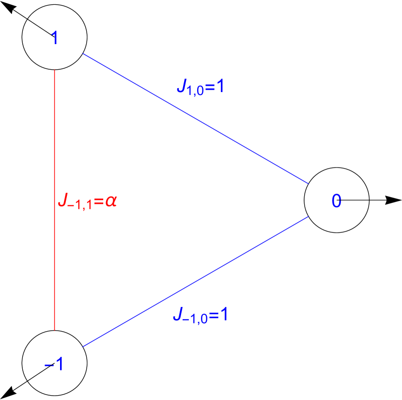
Figure 1: The spin triangle with $J_{1,0}=J_{-1,0}=1$ and a variable bond $J_{-1,1}=\alpha$. The arrows indicate the coplanar ground state for $\alpha=0.6$, see (27).

As one of the simplest examples illustrating the considerations of Section II we consider three spins ${\mathbf{s}}_{\mu}$ indexed by $\mu\in\{-1,0,1\}$, two AF couplings $J_{1,0}=J_{-1,0}=1$ and a variable bond $J_{-1,1}=\alpha$, see Figure 1. Due to the symmetry w. r. t. the transposition $(1\leftrightarrow-1)$ and (5) its dressed ${\mathbbm{J}}$-matrix assumes the form

$${\mathbbm{J}}(\lambda)=\left(\begin{array}[]{ccc}\lambda&1&\alpha\\ 1&-2\lambda&1\\ \alpha&1&\lambda\\ \end{array}\right)\;.$$ (13)

For negative $\alpha$ this system admits an essentially unique collinear ground state symbolically written as ${\mathbf{s}}_{coll}=(\uparrow\downarrow\uparrow)$. If the variable bond has a small positive value, ${\mathbf{s}}_{coll}$ remains the ground state.

The eigenvalues $j_{\mu}(\lambda)$ and eigenvectors ${\mathbf{e}}_{\mu}(\lambda)$ of (13) can be analytically determined:

$$j_{-1}(\lambda) = \lambda-\alpha$$ (14)

$${\mathbf{e}}_{-1}(\lambda) = (-1,0,1)^{\top}$$ (15)

$$j_{0}(\lambda) = \frac{1}{2}\left(\alpha-\lambda-\sqrt{(\alpha+3\lambda)^{2}+8}\right)$$ (16)

$${\mathbf{e}}_{0}(\lambda) = \left(1,\frac{1}{2}\left(-\alpha-3\lambda-\sqrt{(\alpha+3\lambda)^{2}+8}\right),1\right)^{\top}$$ (17)

$$j_{1}(\lambda) = \frac{1}{2}\left(\alpha-\lambda+\sqrt{(\alpha+3\lambda)^{2}+8}\right)$$ (18)

$${\mathbf{e}}_{1}(\lambda) = \left(1,\frac{1}{2}\left(-\alpha-3\lambda+\sqrt{(\alpha+3\lambda)^{2}+8}\right),1\right)^{\top}\;.$$ (19)

The second eigenvalue $j_{0}(\lambda)$ has a smooth maximum at

$$\lambda_{0}=-\frac{1}{3}(\alpha+1)\;,$$ (20)

and intersects the line $j_{-1}(\lambda)$ at

$$\lambda_{1}=\frac{\alpha^{2}-1}{3\alpha}\;.$$ (21)

The equation $\lambda_{0}=\lambda_{1}$ defines the critical value

$$\alpha_{c}=\frac{1}{2}\;.$$ (22)

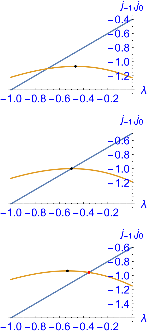
Figure 2: The intersection between $j_{-1}(\lambda)$ (blue line) and $j_{0}(\lambda)$ (orange curve) for the values $\alpha=0.4$, $\alpha=0.5$ and $\alpha=0.6$ (from top to bottom). The smooth maximum of $j_{0}(\lambda)$ is indicated by a black dot, the maximum of $j_{min}(\lambda)$ by a red dot if it differs from that of $j_{-1}(\lambda)$.

It turns out that $j_{min}(\lambda)=\mbox{Min}\left(j_{-1}(\lambda),j_{0}(\lambda)\right)$. If $\lambda_{0}>\lambda_{1}$ or, equivalently, $\alpha<\alpha_{c}=1/2$, then the smooth maximum of $j_{-1}(\lambda)$ coincides with the maximum of $j_{min}(\lambda)$, see Figure 2, top panel. If $\lambda_{0}<\lambda_{1}$ or, equivalently, $\alpha>\alpha_{c}=1/2$, then the maximum of $j_{min}(\lambda)$ occurs at the intersection of $j_{-1}(\lambda)$ and $j_{0}(\lambda)$ , see Figure 2, bottom panel. The boundary between these cases is given by the equation $\lambda_{0}=\lambda_{1}$ or, equivalently, $\alpha=\alpha_{c}=1/2$ and corresponds to the case where the smooth maximum of $j_{-1}(\lambda)$ coincides with the intersection of $j_{-1}(\lambda)$ and $j_{0}(\lambda)$ , see Figure 2, middle panel.

It is clear that in the case $\alpha>\alpha_{c}=1/2$ the eigenspace ${\mathcal{W}}_{min}(\hat{\lambda})$ of ${\mathbbm{J}}(\hat{\lambda})$ is two-dimensional and hence we expect a coplanar ground state in this case. To verify this expectation we consider the matrix

$$W=\left(\begin{array}[]{cc}-1&-1\\ 0&2\alpha\\ 1&-1\\ \end{array}\right)\;,$$ (23)

the columns of which span ${\mathcal{W}}_{min}(\hat{\lambda})$ such that the first column is an eigenvector of $\Pi$ with eigenvalue $-1$ and the second one analogously with eigenvalue $+1$. According to Section II we have to solve the system of equations (11) for the unknown matrix entries of

$$\Delta=\left(\begin{array}[]{cc}\delta_{11}&\delta_{12}\\ \delta_{12}&\delta_{22}\\ \end{array}\right).$$ (24)

The unique solution reads

$$\Delta=\left(\begin{array}[]{cc}-\frac{1-4\alpha^{2}}{4\alpha^{2}}&0\\ 0&\frac{1}{4\alpha^{2}}\\ \end{array}\right)$$ (25)

and yields a ground state Gram matrix of the form

$$G=\left(\begin{array}[]{ccc}1&-\frac{1}{2\alpha}&\frac{1}{2\alpha^{2}}-1\\ -\frac{1}{2\alpha}&1&-\frac{1}{2\alpha}\\ \frac{1}{2\alpha^{2}}-1&-\frac{1}{2\alpha}&1\\ \end{array}\right).$$ (26)

A possible ground state configuration compatible with this Gram matrix can be, according to (12), chosen as

$${\mathbf{s}}=W\,\sqrt{\Delta}\,R=\left(\begin{array}[]{cc}-\frac{1}{2\alpha}&-\frac{1}{2}\sqrt{4-\frac{1}{\alpha^{2}}}\\ 1&0\\ -\frac{1}{2\alpha}&\frac{1}{2}\sqrt{4-\frac{1}{\alpha^{2}}}\\ \end{array}\right),$$ (27)

where $R\in SO(2)$ represents a rotation with the angle $\pi/2$. An example for $\alpha=0.6$ is shown in Figure 3.

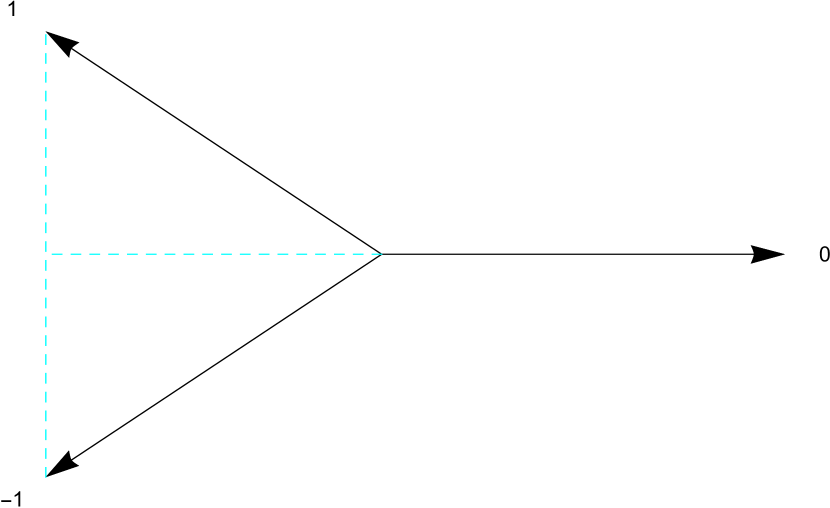
Figure 3: Coplanar ground state of the isosceles triangle with bond $\alpha=0.6$, see also Figure 1. We observe that ${\mathbf{s}}_{1}=R\,{\mathbf{s}}_{-1}$ where $R$ is the reflection on the axis spanned by ${\mathbf{s}}_{0}$.

We will investigate the isolated/cooperative nature of the ground states. The symmetry in question is the linear representation $\Pi$ of the transposition $\pi=(1\leftrightarrow-1)$. According to (15) the eigenvector ${\mathbf{e}}_{-1}(\lambda)=(-1,0,1)^{\top}$ is independent of ${\lambda}$ and has the eigenvalue $-1$ w. r. t. $\Pi$. The other two eigenvectors of ${\mathbbm{J}}(\hat{\lambda})$ belong to the eigenspace of $\Pi$ corresponding to the eigenvalue $+1$. For $\alpha>\alpha_{c}=1/2$ the ground state ${\mathbf{s}}$ is a proper superposition of the first two eigenvectors and hence these ground states are cooperative according to Definition 1.

For $\alpha>\alpha_{c}=1/2$ all coplanar ground states have the same symmetry properties as the ground state shown in Figure 3 for $\alpha=0.6$: The spin vector ${\mathbf{s}}_{1}$ is given by the reflection $R\,{\mathbf{s}}_{-1}$ on the axis spanned by ${\mathbf{s}}_{0}$.

The reasons for these symmetry properties can best be understood by exploiting the fact that ${\mathbf{s}}$ is a symmetric ground state w. r. t. $\Pi$. This means that $\Pi\,{\mathbf{s}}={\mathbf{s}}\,R$ with a suitable $R\in O(2)$, see Section II. ${\mathbf{s}}_{0}$ is left fixed by $\Pi$, hence $R={\mathbbm{1}}$ or $R$ is the reflection on the axis spanned by ${\mathbf{s}}_{0}$. The first possibility would mean that ${\mathbf{s}}$ is isolated contrary to what we have already established. We thus conclude that the swapping of ${\mathbf{s}}_{1}$ and ${\mathbf{s}}_{-1}$ is compensated by the reflection $R$ as shown in Figure 3.

Finally, we consider the ground state energy as a function of $\alpha$. For $\alpha\leq\alpha_{c}=1/2$ the collinear ground state ${\mathbf{s}}_{coll}=(\uparrow\downarrow\uparrow)$ has the energy

$$E_{min}=\alpha-2\;,$$ (28)

see the blue line in Figure 4. For $\alpha>\alpha_{c}=1/2$ the coplanar ground state energy can be calculated as

$$E_{min}=-\alpha-\frac{1}{2\alpha}\;,$$ (29)

see the red curve in Figure 4. In the asymptotic limit $\alpha\rightarrow\infty$ the ground state approaches the form ${\mathbf{s}}=((1,0),(0,1),(-1,0))^{\top}$ with a minimal energy of

$$E_{min}=-\alpha\;,$$ (30)

see the red dashed line in Figure 4.

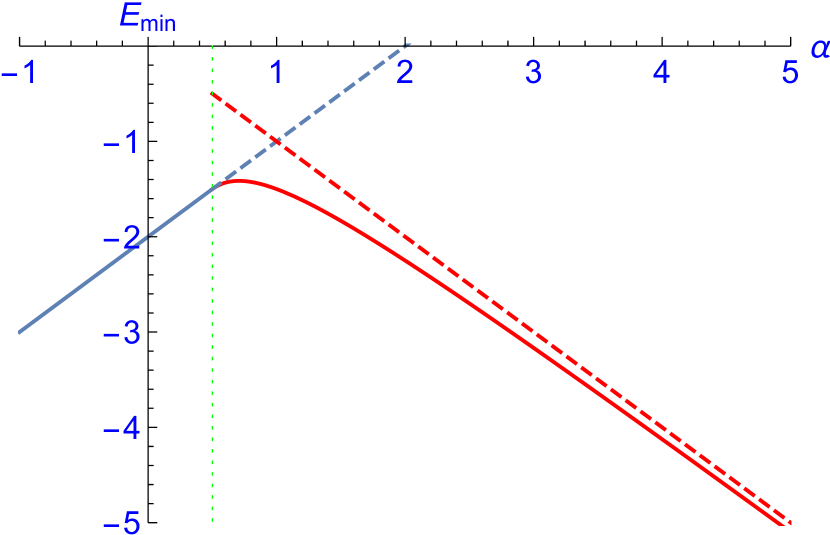
Figure 4: The ground state energy $E_{min}$ as a function of the diagonal bond coupling parameter $\alpha$. For $\alpha\leq\alpha_{c}=1/2$ the minimal energy is given by (28) (blue line) according to the collinear ground state ${\mathbf{s}}_{coll}$. For $\alpha>\alpha_{c}=1/2$ the coplanar cooperative ground state with minimal energy (29) assumes the role of the ground state (red curve). Its asymptotic limit (30) is given by the red dashed line.

III.2 Square with diagonal bond

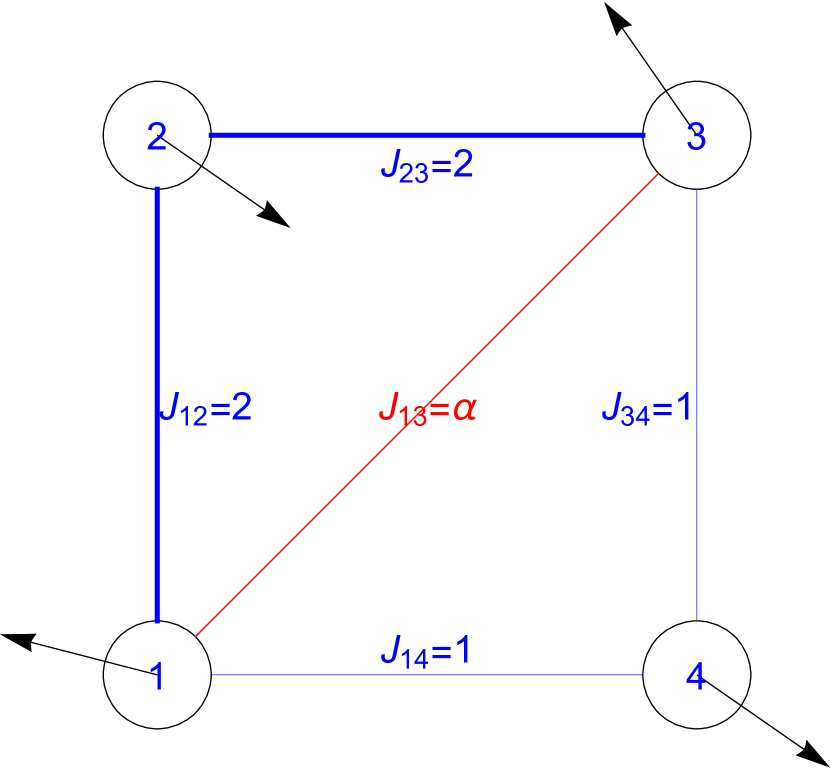
Figure 5: The spin square with $J_{12}=J_{23}=2$ and $J_{34}=J_{41}=1$ and a variable diagonal bond $J_{13}=\alpha$. The arrows indicate the coplanar ground state for $\alpha=1.6$, see (40).

We consider a square with AF couplings $J_{12}=J_{23}=2$ and $J_{34}=J_{41}=1$ and a variable diagonal bond $J_{13}=\alpha$, see Figure 5. Due to the symmetry w. r. t. the transposition $(1\leftrightarrow 3)$ and (5) its dressed ${\mathbbm{J}}$-matrix assumes the form

$${\mathbbm{J}}(\boldsymbol{\lambda})=\left(\begin{array}[]{cccc}\lambda_{1}&2&\alpha&1\\ 2&\lambda_{2}&2&0\\ \alpha&2&\lambda_{1}&1\\ 1&0&1&-2\lambda_{1}-\lambda_{2}\\ \end{array}\right)\;.$$ (31)

The AF square without diagonal bond is a bipartite system and admits an essentially unique collinear ground state symbolically written as ${\mathbf{s}}_{coll}=(\uparrow\downarrow\uparrow\downarrow)$. If a negative diagonal bond $\alpha$ is added to the square, ${\mathbf{s}}_{coll}$ remains the ground state. This holds even for small positive values of $\alpha$.

The eigenvalues of (31) can be analytically determined. The first one reads $j_{1}(\boldsymbol{\lambda})=\lambda_{1}-\alpha$ with eigenvector $(-1,0,1,0)^{\top}$, but the other three eigenvalues are too involved to be represented here. The collinear ground state corresponds to a smooth maximum of a certain eigenvalue henceforward denoted by $j_{2}(\boldsymbol{\lambda})$. This maximum is attained at

$$\lambda_{1}=-\frac{\alpha}{2},\;\lambda_{2}=1+\frac{\alpha}{2}\;,$$ (32)

see Figure 6. It turns out that the minimal eigenvalue $j_{min}(\boldsymbol{\lambda})$ is given by $\mbox{Min}\left(j_{1}(\boldsymbol{\lambda}),j_{2}(\boldsymbol{\lambda})\right)$. Recall that the ground states can be obtained by the unique maximum of $j_{min}(\boldsymbol{\lambda})$. If the smooth maximum of $j_{2}(\boldsymbol{\lambda})$ is also the maximum of $j_{min}(\boldsymbol{\lambda})$ the ground state is collinear, see the top panel of Figure 6. Otherwise the maximum of $j_{min}(\boldsymbol{\lambda})$ can be found at the highest point of the curve given by

$$\lambda_{1}=-\frac{\sqrt{4\alpha\left(\alpha+2\lambda_{2}\right)\left(\alpha^{2}+2\alpha\lambda_{2}-11\right)+169}-2\alpha\left(2\alpha+\lambda_{2}\right)+13}{6\alpha},$$ (33)

that represents the intersection between $j_{1}(\boldsymbol{\lambda})$ and $j_{2}(\boldsymbol{\lambda})$, see the bottom panel of Figure 6. This case corresponds to a coplanar ground state as we will see below. The transition between the two cases is given by the condition that the smooth maximum of $j_{2}(\boldsymbol{\lambda})$ lies on the curve (33), see the middle panel of Figure 6. This condition gives the critical value $\alpha_{c}>0$ as the positive common solution of (32) and (33):

$$\alpha_{c}=\frac{3}{2}\;.$$ (34)

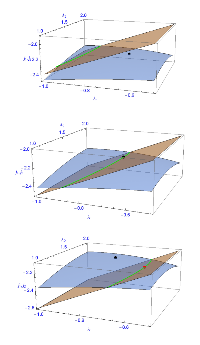
Figure 6: The intersection between $j_{1}(\boldsymbol{\lambda})$ (dark orange plane) and $j_{2}(\boldsymbol{\lambda})$ (blue surface) for the values $\alpha=1.4$, $\alpha=1.5$ and $\alpha=1.6$ (from top to bottom) marked by a green curve. The smooth maximum of $j_{2}(\boldsymbol{\lambda})$ is indicated by a black dot, the maximum of $j_{min}(\boldsymbol{\lambda})$ by a red dot if it differs from that of $j_{2}(\boldsymbol{\lambda})$.

The case $\alpha>\alpha_{c}$ is remarkable in that it differs from the usual picture where the graph of $j_{min}(\boldsymbol{\lambda})$ has a conical structure in the infinitesimal neighbourhood of its maximum which leads to the above mentioned effect called “avoided level crossing". In our case the tangent structure of $j_{min}(\boldsymbol{\lambda})$ at its maximum is rather a wedge with a horizontal edge, see Figure 7.

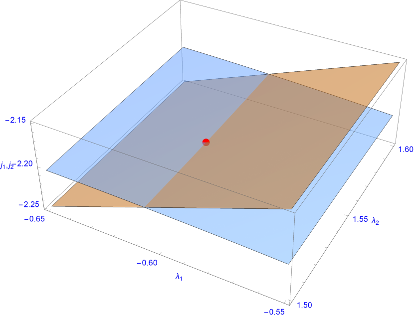
Figure 7: The infinitesimal neighbourhood of the maximum of $j_{min}(\boldsymbol{\lambda})$ for $\alpha=1.6$ corresponding to the bottom panel of Figure 6. Contrary to appearances the blue plane is not horizontal but has a small slope.

It remains to determine the coplanar ground states in the case $\alpha>\alpha_{c}=\frac{3}{2}$. After a short calculation it follows that at the curve given by (33) the eigenvalue $j_{1}(\boldsymbol{\lambda})=j_{2}(\boldsymbol{\lambda})$ assumes its maximum at

$$\hat{\lambda}_{2}=\frac{15-2\alpha^{2}}{4\alpha}\;.$$ (35)

The corresponding two-dimensional eigenspace ${\mathcal{W}}_{min}(\hat{\boldsymbol{\lambda}})$ of ${\mathbbm{J}}(\hat{\boldsymbol{\lambda}})$ is spanned by the columns of

$$W=\left(\begin{array}[]{cc}-\frac{3}{\alpha}&-1\\ 1&0\\ 0&1\\ 1&0\\ \end{array}\right).$$ (36)

According to Section II we have to solve the system of equations (11) for the unknown matrix entries of

$$\Delta=\left(\begin{array}[]{cc}\delta_{11}&\delta_{12}\\ \delta_{12}&\delta_{22}\\ \end{array}\right).$$ (37)

The unique solution reads

$$\Delta=\left(\begin{array}[]{cc}1&-\frac{3}{2\alpha}\\ -\frac{3}{2\alpha}&1\\ \end{array}\right)$$ (38)

and yields a ground state Gram matrix of the form

$$G=\left(\begin{array}[]{cccc}1&-\frac{3}{2\alpha}&\frac{9}{2\alpha^{2}}-1&-\frac{3}{2\alpha}\\ -\frac{3}{2\alpha}&1&-\frac{3}{2\alpha}&1\\ \frac{9}{2\alpha^{2}}-1&-\frac{3}{2\alpha}&1&-\frac{3}{2\alpha}\\ -\frac{3}{2\alpha}&1&-\frac{3}{2\alpha}&1\\ \end{array}\right).$$ (39)

A possible ground state configuration compatible with this Gram matrix can, according to (12), be chosen as

$${\mathbf{s}}=W\,\sqrt{\Delta}=\left(\begin{array}[]{cc}\frac{a(\alpha-3)-b(\alpha+3)}{2\sqrt{2}\alpha}&-\frac{a(\alpha-3)+b(\alpha+3)}{2\sqrt{2}\alpha}\\ \frac{a+b}{2\sqrt{2}}&\frac{b-a}{2\sqrt{2}}\\ \frac{b-a}{2\sqrt{2}}&\frac{a+b}{2\sqrt{2}}\\ \frac{a+b}{2\sqrt{2}}&\frac{b-a}{2\sqrt{2}}\\ \end{array}\right),$$ (40)

where

$$a\equiv\sqrt{2+\frac{3}{\alpha}},\quad\mbox{and }b\equiv\sqrt{2-\frac{3}{\alpha}}\;.$$ (41)

An example for $\alpha=1.6$ is shown in Figure 8.

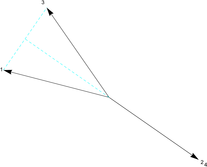
Figure 8: Coplanar ground state of the square with diagonal bond $\alpha=1.6$, see also Figure 5. We observe that ${\mathbf{s}}_{2}={\mathbf{s}}_{4}$ and that ${\mathbf{s}}_{3}=R\,{\mathbf{s}}_{1}$ where $R$ is the reflection on the axis spanned by ${\mathbf{s}}_{2}={\mathbf{s}}_{4}$.

We will investigate the isolated/cooperative nature of the ground states. The symmetry in question is the linear representation $\Pi$ of the transposition $\pi=(1\leftrightarrow 3)$. We have already mentioned the eigenvector $(-1,0,1,0)^{\top}$ of $j_{1}({\boldsymbol{\lambda}})$ that is independent of ${\boldsymbol{\lambda}}$ and has the eigenvalue $-1$ w. r. t. $\Pi$. The other three eigenvectors of ${\mathbbm{J}}(\hat{\boldsymbol{\lambda}})$ belong to the eigenspace of $\Pi$ corresponding to the eigenvalue $+1$. For $\alpha>\alpha_{c}=3/2$ the ground state ${\mathbf{s}}$ is a proper superposition of $e_{-1}(\lambda)$ and $e_{0}(\lambda)$ and hence these ground states are cooperative according to Definition 1.

For $\alpha>\alpha_{c}=3/2$ all coplanar ground states have the same symmetry properties as the ground state shown in Figure 8 for $\alpha=1.6$: Two spin vectors coincide, ${\mathbf{s}}_{2}={\mathbf{s}}_{4}$, and ${\mathbf{s}}_{3}$ is given by the reflection $R\,{\mathbf{s}}_{1}$ on the axis given by ${\mathbf{s}}_{2}={\mathbf{s}}_{4}$.

The reasons for these symmetry properties can best be understood by exploiting the fact that ${\mathbf{s}}$ is a symmetric ground state w. r. t. $\Pi$. This means that $\Pi\,{\mathbf{s}}={\mathbf{s}}\,R$ with a suitable $R\in O(2)$, see Section II. ${\mathbf{s}}_{2}$ and ${\mathbf{s}}_{4}$ are left fixed by $\Pi$, hence $R={\mathbbm{1}}$ if $({\mathbf{s}}_{2},{\mathbf{s}}_{4})$ would be linearly independent. This would mean that ${\mathbf{s}}$ is isolated contrary to what we have already established. We thus conclude ${\mathbf{s}}_{2}={\mathbf{s}}_{4}$ since ${\mathbf{s}}_{2}=-{\mathbf{s}}_{4}$ can be excluded by arguing with the requirement of minimal energy. Further, we conclude that $R$ leaves ${\mathbf{s}}_{2}$ invariant and hence must be a reflection on the line given by multiples of ${\mathbf{s}}_{2}$.

Finally, we consider the ground state energy as a function of $\alpha$. For $\alpha\leq\alpha_{c}=3/2$ the collinear ground state ${\mathbf{s}}_{coll}=(\uparrow\downarrow\uparrow\downarrow)$ has the energy

$$E_{min}=\alpha-6\;,$$ (42)

see the blue line in Figure 9. For $\alpha>\alpha_{c}=3/2$ the coplanar ground state energy can be calculated as

$$E_{min}=-\alpha-\frac{9}{2\alpha}\;,$$ (43)

see the red curve in Figure 9. In the asymptotic limit $\alpha\rightarrow\infty$ the ground state approaches the form ${\mathbf{s}}=((1,0),(0,1),(-1,0),(0,1))^{\top}$ with a minimal energy of

$$E_{min}=-\alpha\;,$$ (44)

see the red dashed line in Figure 9.

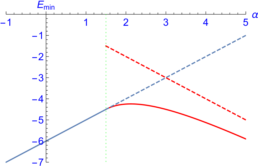
Figure 9: The ground state energy $E_{min}$ as a function of the diagonal bond coupling parameter $\alpha$. The critical value $\alpha_{c}=3/2$ is indicated by a vertical dotted green line. For $\alpha\leq\alpha_{c}$ the minimal energy is given by (42) (blue line) according to the collinear ground state ${\mathbf{s}}_{coll}$. For $\alpha>\alpha_{c}$ the coplanar cooperative ground state with minimal energy (43) assumes the role of the ground state (red curve). Its asymptotic limit (44) is given by the red dashed line.

III.3 Almost regular Cube

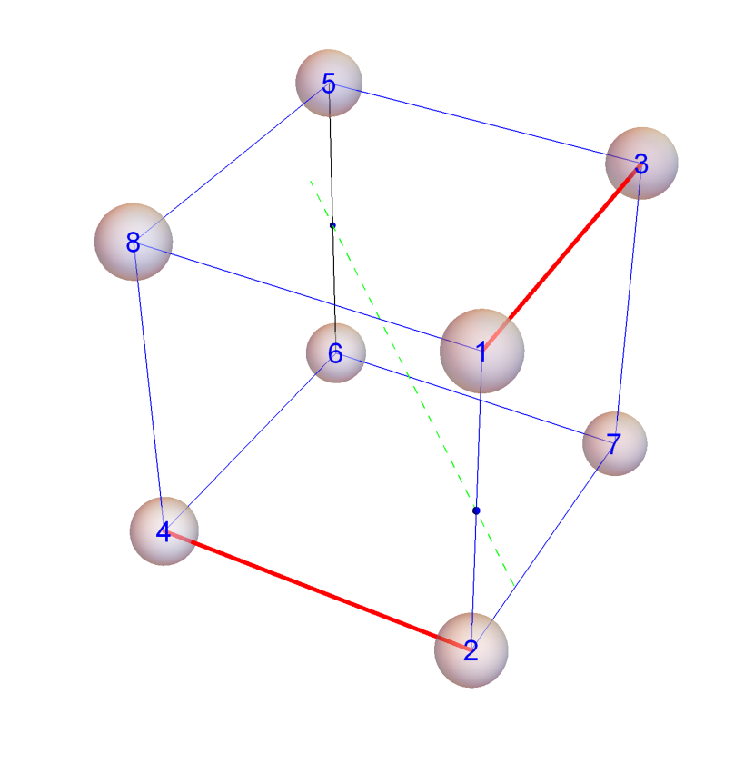
Figure 10: The cube with AF coupling $J_{\mu\nu}=1$ (blue lines) except one variable coupling parameter $J_{24}=J_{13}=\alpha$ (red thick lines). This spin system is invariant under the rotation about the dashed green axis with an angle of $180^{\circ}$.

We consider a cube with AF coupling $J_{\mu\nu}=1$ except one variable coupling parameter $J_{24}=J_{13}=\alpha$, see Figure 10. The system has the symmetry $\pi=(1\leftrightarrow 2,3\leftrightarrow 4,5\leftrightarrow 6,7\leftrightarrow 8)$ that can be geometrically interpreted as a rotation about a suitable axis with an angle of $180^{\circ}$, see Figure 10. As usual, $\Pi$ denotes the standard representation of $\pi$ by an $8\times 8$-matrix. The enumeration of the spin sites is adapted to this symmetry. The AF cube ($\alpha>0$) admits a collinear ground state ${\mathbf{s}}_{coll}$ symbolically written as $(\uparrow\downarrow\downarrow\uparrow\uparrow\downarrow\uparrow\downarrow)$ that remains the ground state even for small negative values of $\alpha$.

Taking into account the symmetry $\pi$ the dressed ${\mathbbm{J}}$-matrix assumes the form

$${\mathbbm{J}}({\boldsymbol{\lambda}})=\left(\begin{array}[]{cccccccc}\lambda_{1}&1&\alpha&0&0&0&0&1\\ 1&\lambda_{1}&0&\alpha&0&0&1&0\\ \alpha&0&\lambda_{2}&0&1&0&1&0\\ 0&\alpha&0&\lambda_{2}&0&1&0&1\\ 0&0&1&0&\lambda_{3}&1&0&1\\ 0&0&0&1&1&\lambda_{3}&1&0\\ 0&1&1&0&0&1&\lambda_{4}&0\\ 1&0&0&1&1&0&0&\lambda_{4}\\ \end{array}\right)\;,$$ (45)

where $\lambda_{4}\equiv-\lambda_{1}-\lambda_{2}-\lambda_{3}$ due to (5). If we transform ${\mathbbm{J}}({\boldsymbol{\lambda}})$ to the eigenbasis of $\Pi$ that is formed by the columns of the following matrix

$$U=\frac{1}{\sqrt{2}}\left(\begin{array}[]{rrrrrrrr}1&0&0&0&1&0&0&0\\ 1&0&0&0&-1&0&0&0\\ 0&1&0&0&0&1&0&0\\ 0&1&0&0&0&-1&0&0\\ 0&0&1&0&0&0&1&0\\ 0&0&1&0&0&0&-1&0\\ 0&0&0&1&0&0&0&1\\ 0&0&0&1&0&0&0&-1\\ \end{array}\right)\;,$$ (46)

we obtain the block matrix

$$U^{\top}\,{\mathbbm{J}}({\boldsymbol{\lambda}})\,U=$$

$$\left(\begin{array}[]{cccccccc}\lambda_{1}+1&\alpha&0&1&0&0&0&0\\ \alpha&\lambda_{2}&1&1&0&0&0&0\\ 0&1&\lambda_{3}+1&1&0&0&0&0\\ 1&1&1&\lambda_{4}&0&0&0&0\\ 0&0&0&0&\lambda_{1}-1&\alpha&0&-1\\ 0&0&0&0&\alpha&\lambda_{2}&1&1\\ 0&0&0&0&0&1&\lambda_{3}-1&-1\\ 0&0&0&0&-1&1&-1&\lambda_{4}\\ \end{array}\right).$$ (47)

Its characteristic polynomial $p(x,{\boldsymbol{\lambda}})$ can hence be split into two factors $p=p_{1}\,p_{2}$, such that the zeroes of $p_{1}$ are the eigenvalues of parity $+1$ and the zeroes of $p_{2}$ those of parity $-1$. The data for the collinear ground state can be directly obtained by inserting ${\mathbf{s}}_{coll}$ into (3) and calculating the $\lambda_{i}$ and the minimal eigenvalue of ${\mathbbm{J}}({\boldsymbol{\lambda}})$. The result reads

$$\hat{\jmath} = \frac{1}{2}(-\alpha-5),\quad E_{min}=2(-\alpha-5),$$ (48)

$$\lambda_{1} = \lambda_{2}=\frac{\alpha-1}{2},\quad\lambda_{3}=\lambda_{4}=\frac{1-\alpha}{2}\;.$$ (49)

Inserting these values of the components of ${\boldsymbol{\lambda}}$ into $p_{2}$ gives a polynomial $p_{2}(x,\alpha)$. The condition $p_{2}(x,\alpha)=\frac{\partial p_{2}(x,\alpha)}{\partial x}=0$ characterizes the occurrence of a degenerate eigenvalue of ${\mathbbm{J}}({\boldsymbol{\lambda}})$. Inserting the value $x=\hat{\jmath}=\frac{1}{2}(-\alpha-5)$ from (48) yields the critical value for $\alpha$

$$\alpha_{c}^{(1)}=-\frac{3}{5}$$ (50)

that separates the collinear from the coplanar ground states.

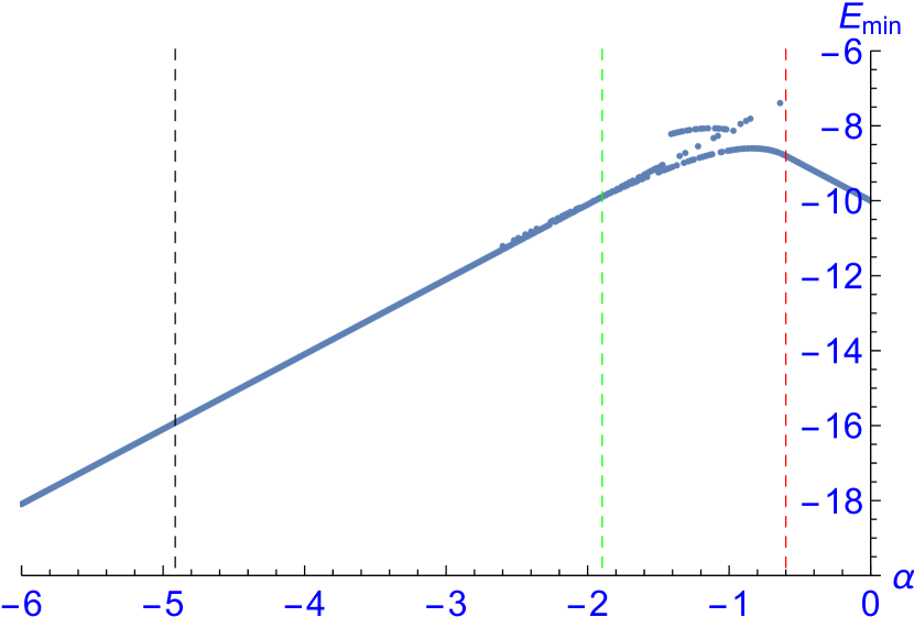
Figure 11: The numerically determined ground state energy $E_{min}$ of the almost regular cube as a function of the variable bond coupling parameter $\alpha$. Some spurious configurations yield energies above the minimal one. The critical values $\alpha_{c}^{(i)},\;i=1,2,3,$ are indicated by vertical dashed lines. At these values the nature of the ground state changes in a manner explained in the text.

The closer investigation of coplanar ground states leads us to the limits of the analytical treatment of the problem, even if we use computer algebraic methods. At any case numerical calculations have to serve as an auxiliary tool. The main result is the occurrence of two further critical values

$$\alpha_{c}^{(2)}\approx-1.8963,\quad\mbox{and }\alpha_{c}^{(3)}\approx-4.8208\;,$$ (51)

such that for $\alpha_{c}^{(2)}<\alpha<\alpha_{c}^{(1)}$ and $\alpha<\alpha_{c}^{(3)}$ we obtain isolated ground states and for $\alpha_{c}^{(3)}<\alpha<\alpha_{c}^{(2)}$ cooperative ones.

For a first orientation we numerically calculate the ground state energy $E_{min}$ for values $-6<\alpha<0$ of the variable bond strength, see Figure 11. We use a very simple algorithm that starts with a random spin configuration and successively lowers its energy by correcting the single spins ${\mathbf{s}}_{\mu}$ according to (3). The linear domain $-0.6<\alpha<0$ corresponds to the collinear ground state ${\mathbf{s}}_{coll}=(\uparrow\downarrow\downarrow\uparrow\uparrow\downarrow\uparrow\downarrow)$ and $E_{min}$ given by (48). It may happen that the sketched numerical procedure does not yield an approximation of the true ground state, but is trapped in the neighbourhood of a local energy minimum or pseudo-minimum. This can be seen in Figure 11 where a couple of connected points lying nearly on a line is markedly above the energy minimum. We have not tried to get rid of these spurious ground states but rather will use them as a hint to the position of certain cooperative states that will become ground states for values of $\alpha_{c}^{(3)}<\alpha<\alpha_{c}^{(2)}$. The other spurious points forming a concave curve are neglected.

In order to analyze the isolated coplanar ground states we first note that for alternating spin configurations ${\mathbf{s}}_{\mu}=-{\mathbf{s}}_{\mu+1},\;\mu=1,3,5,7$ the energy can be written as

$$E=\frac{1}{2}\left(\begin{array}[]{r}{\mathbf{s}}_{1}\\ -{\mathbf{s}}_{1}\\ {\mathbf{s}}_{3}\\ -{\mathbf{s}}_{3}\\ {\mathbf{s}}_{5}\\ -{\mathbf{s}}_{5}\\ {\mathbf{s}}_{7}\\ -{\mathbf{s}}_{7}\\ \end{array}\right)^{\top}\left(\begin{array}[]{cccccccc}0&1&\alpha&0&0&0&0&1\\ 1&0&0&\alpha&0&0&1&0\\ \alpha&0&0&0&1&0&1&0\\ 0&\alpha&0&0&0&1&0&1\\ 0&0&1&0&0&1&0&1\\ 0&0&0&1&1&0&1&0\\ 0&1&1&0&0&1&0&0\\ 1&0&0&1&1&0&0&0\\ \end{array}\right)\left(\begin{array}[]{r}{\mathbf{s}}_{1}\\ -{\mathbf{s}}_{1}\\ {\mathbf{s}}_{3}\\ -{\mathbf{s}}_{3}\\ {\mathbf{s}}_{5}\\ -{\mathbf{s}}_{5}\\ {\mathbf{s}}_{7}\\ -{\mathbf{s}}_{7}\\ \end{array}\right)$$ (52)

$$=\frac{1}{2}\left(\begin{array}[]{c}{\mathbf{s}}_{1}\\ {\mathbf{s}}_{3}\\ {\mathbf{s}}_{5}\\ {\mathbf{s}}_{7}\\ \end{array}\right)^{\top}\left(\begin{array}[]{rrrr}-2&2\alpha&0&-2\\ 2\alpha&0&2&2\\ 0&2&-2&-2\\ -2&2&-2&0\\ \end{array}\right)\left(\begin{array}[]{c}{\mathbf{s}}_{1}\\ {\mathbf{s}}_{3}\\ {\mathbf{s}}_{5}\\ {\mathbf{s}}_{7}\\ \end{array}\right)\equiv\frac{1}{2}\tilde{\mathbf{s}}^{\top}\tilde{\mathbbm{J}}\tilde{\mathbf{s}}\;.$$ (53)

Hence we may use the $4\times 4$-matrix $\tilde{\mathbbm{J}}$ in (53) as the undressed ${\mathbbm{J}}$-matrix of an auxiliary $N=4$ spin system and apply the methods described in this paper. The unfamiliar diagonal terms should not bother us.

First we look for degenerate eigenvalues of $\tilde{\mathbbm{J}}({\boldsymbol{\lambda}})$ and hence for solutions of

$$0=p(x,{\boldsymbol{\lambda}})=\frac{\partial p(x,{\boldsymbol{\lambda}})}{\partial x}=\frac{\partial p(x,{\boldsymbol{\lambda}})}{\partial\lambda_{i}},\quad i=1,2,3\;,$$ (54)

where $p(x,{\boldsymbol{\lambda}})$ is the characteristic polynomial $p(x,{\boldsymbol{\lambda}})=\det\left(\tilde{\mathbbm{J}}({\boldsymbol{\lambda}})-x\,{\mathbbm{1}}\right)$. The solutions of (54) depend on a free parameter and can be written in the form $\lambda_{i}=L_{i}(x),\;i=1,2,3$. This is in accordance with the dimension $L-2=1$ of the variety $j_{min}^{(2)}({\boldsymbol{\lambda}})$ due to the rules of avoided level crossing, see Section II.

Recall that $x$ represents the eigenvalue $j_{min}({\boldsymbol{\lambda}})$ of $\tilde{\mathbbm{J}}({\boldsymbol{\lambda}})$ and hence has to be chosen as the maximum of all values $x$ such that $L_{i}(x)$ is a smooth parameter representation. It turns out that all $L_{i}(x)$ contain a square root of the form $\sqrt{f(x)}$ where $f(x)$ is the fourth order polynomial

$$f(x) = \left(16\alpha^{2}+8\alpha+3\right)(\alpha-1)^{4}$$ (55)

$$-4\left(8\alpha^{2}+1\right)(\alpha-1)^{3}x$$

$$-4(6\alpha+1)(\alpha-1)^{2}x^{2}$$

$$+16\alpha\left(2\alpha^{2}-\alpha+1\right)x^{3}-16\alpha^{2}x^{4}\;.$$

Hence the maximal value $\hat{\jmath}$ is given by a suitable zero of (55) that can be calculated analytically but is too complex to be given here. The corresponding energy $E_{iso}(\alpha)=\frac{N}{2}\hat{\jmath}=2\hat{\jmath}$ is plotted in Figure 12. This result is already very close to the numerical one, see Figure 11, but we will see that for $\alpha_{c}^{(3)}<\alpha<\alpha_{c}^{(2)}$ the cooperative ground states will yield a smaller energy.

The collinear state ${\mathbf{s}}_{asy}=(\uparrow\downarrow\uparrow\downarrow\downarrow\uparrow\downarrow\uparrow)$ yields the energy $E_{asy}=2\alpha-6$ that is asymptotically assumed for $\alpha\to-\infty$, see Figure 12.

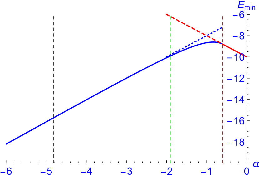
Figure 12: The analytically determined ground state energy $E_{iso}$ of the almost regular cube as a function of the variable bond coupling parameter $\alpha$ for isolated coplanar ground states (blue curve). For $\alpha\to-\infty$ the ground state energy is asymptotically given by $E_{asy}=2\alpha-6$ (dashed blue line). As in Figure 11 the critical values $\alpha_{c}^{(i)},\;i=1,2,3,$ are indicated by vertical dashed lines. The energy of the collinear ground state according to (48) is represented by a red solid line in the domain $-\frac{3}{5}<\alpha<0$ and for smaller values of $\alpha$ by a dashed red line.

The isolated ground state configurations corresponding to the minimal energy can also be analytically determined but only for chosen values of $\alpha$. As an example we display the ground state configuration for $\alpha=-1$, see Figure 13. This example is remarkable in so far as the ground state configuration can be characterized by a single angle:

$${\mathbf{s}}_{1}\cdot{\mathbf{s}}_{5}=0\quad\mbox{and}$$ (56)

$${\mathbf{s}}_{1}\cdot{\mathbf{s}}_{3}={\mathbf{s}}_{1}\cdot{\mathbf{s}}_{7}=$$ (57)

$$\frac{1}{4}\left(1-\sqrt{5}+\sqrt{2\left(1+\sqrt{5}\right)}\right)=0.326993\ldots$$ (58)

Figure 13: The analytically determined isolated ground state (56) - (58) of the almost regular cube for the value of the variable bond coupling parameter $\alpha=-1$. Only spin vectors with odd numbers are shown, the even ones are obtained by ${\mathbf{s}}_{\mu+1}=-{\mathbf{s}}_{\mu},\;\mu=1,3,5,7$.

Next we consider possible cooperative ground states. There are no principal obstacles to obtaining closed solutions depending on the parameter $\alpha$, but due to the practical limitations of storage and computing times it is only possible to solve the problem for fixed values of $\alpha$. Even with this restriction the intermediate and final results are too complex to be explicitly given.

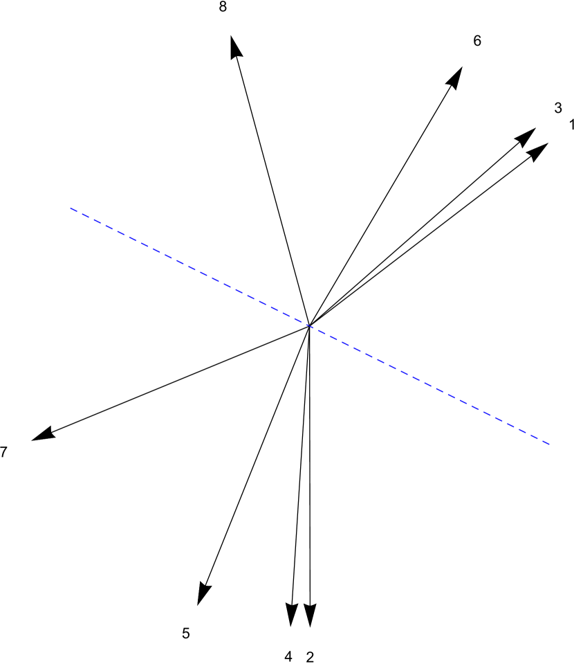
Figure 14: A numerically determined cooperative ground state of the almost regular cube for the value of the variable bond coupling parameter $\alpha=-2$. The symmetry axis is shown as a blue, dashed line.

We return to the $N=8$ spin system and the dressed ${\mathbbm{J}}$-matrix (47). In this case the equations analogous to (54) have solutions of the form $\lambda_{i}=K_{i}(x,\lambda_{3}),\;i=1,2,$ corresponding to a two-dimensional intersection of eigenvalue varieties belonging to different eigenspaces of the symmetry $\Pi$. This is in accordance with the dimension $L-1=2$ of the variety $j_{min}^{(2)}({\boldsymbol{\lambda}})$ due to symmetry-allowed level crossing, see Section II.

In the following we consider the example $\alpha=-2$ that is, however, typical for other integer or half integer values of $\alpha$. The function $\lambda_{2}=K_{2}(x,\lambda_{3})$ has the form of a certain double root of a polynomial $P_{2}(x,\lambda_{2},\lambda_{3})$. The corresponding equations $0=P_{2}(x,\lambda_{2},\lambda_{3})=\frac{\partial P_{2}(x,\lambda_{2},\lambda_{3})}{\partial\lambda_{2}}$ can be used to eliminate $\lambda_{2}$ with the result $Q(x,\lambda_{3})=0$, where $Q$ is the resultant of $P_{2}$ and its derivative w. r. t. $\lambda_{2}$. Actually $Q$ is a polynomial in $x$ and $\lambda_{3}$ of degree $40$. This step thus reduces the intersection of the appropriate eigenvalue varieties of ${\mathbbm{J}}({\boldsymbol{\lambda}})$ to a curve of dimension one. Since $x$ must be maximal within this curve we have the additional equation $\frac{\partial Q(x,\lambda_{3})}{\partial\lambda_{3}}=0$. Together with $Q(x,\lambda_{3})=0$ we can numerically solve for $x$ and obtain $E_{min}=4x=-10.1009\ldots$. Note that the essential use of numerics is confined to the last step of finding roots of polynomial equations. A typical cooperative ground state for $\alpha=-2$ with the same symmetry as in Figure 3 is shown in Figure 14.

Analogously, we have obtained minimal energies $E_{coop}(\alpha)$ for the values $\alpha=-1,-1.5,\ldots,-6$, see Table 1, where also the values of $E_{iso}(\alpha)$ have been displayed. The integer value $E_{iso}=-12$ for $\alpha=-3$ can be explained by the fact that here the isolated coplanar state degenerates into the collinear state ${\mathbf{s}}_{asy}=(\uparrow\downarrow\uparrow\downarrow\downarrow\uparrow\downarrow\uparrow)$ with energy $E(\alpha)=2\alpha-6$.

Table 1: Table of energies $E_{coop}$ and $E_{iso}$ of possible cooperative/isolated ground states for different values of $\alpha$. The ground state energies are shown in bold.

$\alpha$	$E_{coop}$	$E_{iso}$
$-1$	$-8.10796$	$\mathbf{-8.66038}$
$-1.5$	$-9.10359$	$\mathbf{-9.24214}$
$-2$	$\mathbf{-10.1009}$	$-10.0787$
$-2.5$	$\mathbf{-11.0992}$	$-11.0154$
$-3$	$\mathbf{-12.0979}$	$-12.0000$
$-3.5$	$\mathbf{-13.0969}$	$-13.0105$
$-4$	$\mathbf{-14.0962}$	$-14.0359$
$-4.5$	$\mathbf{-15.0956}$	$-15.0703$
$-5$	$-16.0951$	$\mathbf{-16.1102}$
$-5.5$	$-17.0947$	$\mathbf{-17.1536}$
$-6$	$-18.0943$	$\mathbf{-18.1992}$

A cubic fit of the almost linear function $E_{coop}(\alpha)$ intersects the analytically determined function $E_{iso}(\alpha)$ at the points $\alpha_{c}^{(2)}\approx-1.8963$ and $\alpha_{c}^{(3)}\approx-4.8208$, see Figure 15, such that for $\alpha_{c}^{(3)}<\alpha<\alpha_{c}^{(2)}$ the cooperative states represent the true ground states. The phase transition at $\alpha_{c}^{(3)}\approx-4.8208$ would be hardly detectable by purely numerical methods.

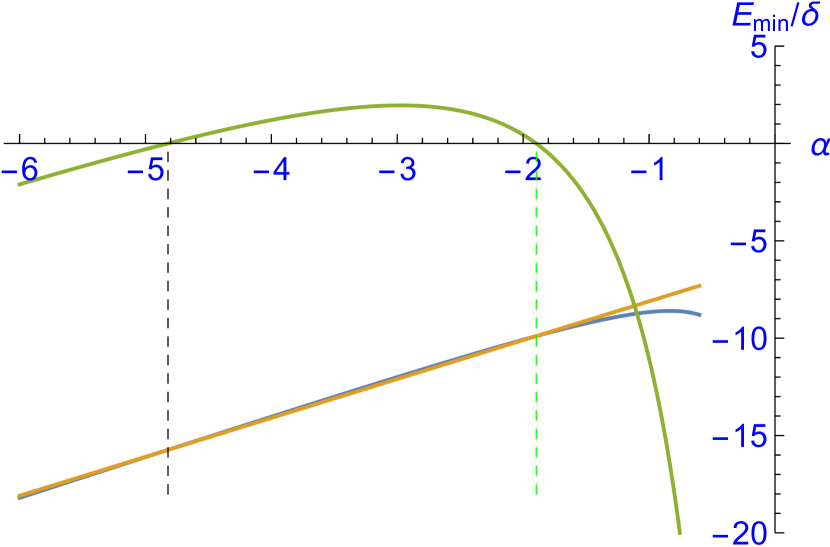
Figure 15: The two curves $E_{iso}(\alpha)$ (blue curve) and $E_{coop}(\alpha)$ (orange curve) and their intersections at $\alpha_{c}^{(2)}\approx-1.8963$ and $\alpha_{c}^{(3)}\approx-4.8208$ indicated by vertical dashed lines. Since the two curves can hardly be distinguished we have also shown the magnified difference $\delta\equiv 20(E_{iso}(\alpha)-E_{coop}(\alpha))$ (green curve).

IV Summary and Outlook

We have revisited the theory of ground states published three years ago and added the novel aspect of the isolated/cooperative distinction for ground states in the case of an involutary symmetry. This distinction has been illustrated by three examples, which also have other interesting features: The isosceles triangle, the square with a diagonal bond and the almost regular cube. All examples possess a variable bond parameter $\alpha$, and show a phase transition between collinear and coplanar ground states at some critical values of $\alpha=\alpha_{c}$. In all cases the critical values lie beyond the “trivial domain" where the collinear ground state minimizes the energy of every individual bond. Thus we have a coexistence of competing interactions and collinear ground states for

• the triangle and $0<\alpha<1/2$,

• the square and $0<\alpha<3/2$, and

• the cube and $-3/5<\alpha<0$.

Moreover, the gauge parameters of the cube satisfy the remarkable identity $\lambda_{1}=\lambda_{2}=-\lambda_{3}=-\lambda_{4}$ for the collinear ground state domain $-3/5=\alpha_{c}<\alpha$. All examples possess cooperative coplanar ground states for suitable values of $\alpha$; the cube has additionally isolated coplanar ground states and phase transitions between these two types at certain further critical values of $\alpha$.

A natural generalization of these studies would consist in considering a larger group ${\sf G}$ of symmetries. If ${\sf G}$ is generated by $d$ commuting involutary symmetries the generalization appears to be straight forward. Instead of two orthogonal subspaces with different parity we would have $2^{d}$ ones and a corresponding variety of different isolated and cooperative coplanar ground states. A further generalization, however, would be faced with the following complication: Any non-involutary symmetry would possess complex eigenvalues of the form $e^{{\sf i}\,\alpha}$ with $\alpha\neq 0,\pi$ and the corresponding complex eigenspaces. Since the eigenspaces ${\mathcal{W}}_{min}(\hat{\boldsymbol{\lambda}})$ considered for the ground state problem have to be real we cannot simply transfer the results of the present paper to the general case of a symmetry group.

Another possible generalization would consist of extending the isolated/cooperative distinction and the application of the avoided level crossing rules to three-dimensional ground states.

References

- (1) M. Axenovich and M. Luban, Exact ground state properties of the classical Heisenberg model for giant magnetic molecules, Phys. Rev. B 63, 100407(R) (2003)
- (2) A. Proykova and D. Stauffer, Classical simulations of magnetic structures for chromium clusters: size effects, Cent. Eur. J. Phys. 3 (2), 209 - 220 (2005)
- (3) C. Schröder, H.-J. Schmidt, J. Schnack, and M. Luban, Metamagnetic Phase Transition of the Antiferromagnetic Heisenberg Icosahedron, Phys. Rev. Lett. 94 (20), 207203 (2005)
- (4) N. P. Konstantinidis et al, Magnetism on a Mesoscopic Scale: Molecular Nanomagnets Bridging Quantum and Classical Physics, J. Phys.: Conf. Ser. 303, 012003 (2011)
- (5) A. P. Popov, A. Rettori, and M. G. Pini, Discovery of metastable states in a finite-size classical one-dimensional planar spin chain with competing nearest- and next-nearest-neighbor exchange couplings, Phys. Rev. B 90, 134418 (2014)
- (6) K. Ch. Mondal et al, A Strongly Spin-Frustrated Complex with a Canted Intermediate Spin Ground State of or , Chem. Eur. J. 21, 10835 - 10842 (2015)
- (7) G. Kamieniarz, W. Florek, and M. Antkowiak, Universal sequence of ground states validating the classification of frustration in antiferromagnetic rings with a single bond defect, Phys. Rev. B 92, 140411(R) (2015)
- (8) A. P. Popov, A. Rettori, and M. G. Pini, Spectrum of noncollinear metastable configurations of a finite-size discrete planar spin chain with a collinear ferromagnetic ground state, Phys. Rev. B 92, 024414 (2015)
- (9) V. K. Henner, A. Klots, and T. Belozerova, Simulation of Pake doublet with classical spins and correspondence between the quantum and classical approaches, Eur. Phys. J. B 89, 264 (2016)
- (10) W. Florek, M. Antkowiak, and G. Kamieniarz, Sequences of ground states and classification of frustration in odd-numbered antiferromagnetic rings, Phys. Rev. B 94, 224421 (2016)
- (11) R. J. Woolfson et al, : Synthesis and Characterization of a Regular Homometallic Ring with an Odd Number of Metal Centers and Electrons, Angew. Chem. Int. Ed. 55,8856 - 8859 (2016)
- (12) S. Castillo-Sepúlveda et al, Magnetic Möbius stripe without frustration: Noncollinear metastable states, Phys. Rev. B 96, 024426 (2017)
- (13) N. P. Konstantinidis, Zero-temperature magnetic response of small fullerene molecules at the classical and full quantum limit, J. Magn. Magn. Mater. 449, 55 - 62 (2018)
- (14) A. Baniodeh, N. Magnani, Y. Lan et al, High spin cycles: topping the spin record for a single molecule verging on quantum criticality, npj Quant. Mater. 3, 10 (2018)
- (15) D. V. Dmitriev, V. Ya. Krivnov, J. Richter, and J. Schnack, Thermodynamics of a delta chain with ferromagnetic and antiferromagnetic interactions, Phys. Rev. B 99, 094410 (2019)
- (16) A. P. Singh et al, Molecular spin frustration in mixed-chelate and oxo clusters with high ground state spin values, Polyhedron 176, 114182 (2020)
- (17) H.-J. Schmidt and M. Luban, Classical ground states of symmetric Heisenberg spin systems, J. Phys. A 36, 6351 – 6378 (2003)
- (18) H.-J. Schmidt, Theory of ground states for classical Heisenberg spin systems I, arXiv:cond-mat1701.02489v2, (2017)
- (19) H.-J. Schmidt, Theory of ground states for classical Heisenberg spin systems II, arXiv:cond-mat1707.02859v2, (2017)
- (20) H.-J. Schmidt, Theory of ground states for classical Heisenberg spin systems III, arXiv:cond-mat1707.06512v2, (2017)
- (21) H.-J. Schmidt, Theory of ground states for classical Heisenberg spin systems IV, arXiv:1710.00318v1, (2017)
- (22) W. Florek and A. Marlewski, Spectrum of some arrow-bordered circulant matrix, arXiv:math.CO1905.04807 (2019)
- (23) W. Florek, G. Kamieniarz, and A. Marlewski, Universal lowest energy configurations in a classical Heisenberg model describing frustrated systems with wheel geometry, Phys. Rev. B 100, 054434 (2019)
- (24) J. von Neumann and E. P. Wigner, Über das Verhalten von Eigenwerten bei adiabatischen Prozessen, Phys. Z. 30, 467-470 (1929)
- (25) V. I. Arnold, Mathematical Methods of Classical Mechanics, 2nd ed. , Springer-Verlag, New York, 1989, Appendix 10