Constant-roll in the Palatini–$R^{2}$ models

Abstract

We consider models of a scalar field coupled to quadratic $R\!+\!R^{2}$ gravity in the framework of the Palatini formulation. The resulting Einstein-frame generalized $k$-inflation effective theory is analyzed assuming that the constant-roll condition holds. We focus on a quartic self-interaction potential, a case of particular appeal modelling Higgs inflation, considering the cases of minimal and non-minimal coupling of the inflaton to gravity. For an appropriate range of the model parameters in the large field domain the obtained values for the inflationary observables are found in agreement with current observations.

1 Introduction

The theory of cosmic inflation [1, 2, 3, 4, 5, 6, 7], i.e. a period of quasi–de Sitter expansion of the Universe during the first instants after its birth, was initially motivated by its solution to the problems of traditional Big Bang cosmology, like the observed flatness and large scale CMB temperature uniformity. Nevertheless, its present appeal is that it provides a mechanism through which the tiny primordial inhomogeneities, arising as quantum fluctuations, are allowed to grow and become classical at superhorizon scales [8, 9, 10, 11, 12, 13]. Present experimental efforts focused on the CMB [14, 15], strongly constrain the inflationary spectrum with an increasing accuracy, having narrowed considerably the range of viable inflationary models. Although the power spectrum of scalar perturbations is very nearly scale-invariant and Gaussian, and this agrees with inflationary models in their simplest implementation, in the medium-term future non-Gaussianities might be uncovered through the increasing accuracy of observations. The scalar degree of freedom (inflaton) employed in these models can either be a fundamental scalar field or can arise as an effective scalar degree of freedom incorporated in gravity itself. The latter possibility is realized in the so-called modified gravity models (see for a review [16, 17, 18, 19, 20]) and in particular in the Starobinsky model[1], which is persistently in agreement with observations, regarding its inflationary spectrum. In fact, the Starobinsky model, as well as any theory of gravity with an action $\int\,d^{4}x\,\sqrt{-g}\,f(R)$, can be reformulated as a scalar–tensor theory of gravity with a non-minimal coupling of the effective scalar degree of freedom to the Ricci scalar.

Although known for sometime, the so-called first order or Palatini formulation of gravity [21] has recently received considerable attention [22, 23, 24, 25, 26, 27, 28, 29, 30, 31, 32, 33, 34, 35, 36, 37, 38, 39, 40, 41, 42, 43, 44, 45, 46, 47, 48, 49, 50], since, in the case of scalar fields non-minimally coupled to gravity, it leads to different predictions than the standard (dubbed as metric) formulation. In the Palatini formulation the metric $g_{\mu\nu}$ and the connection $\Gamma_{\mu\nu}^{\rho}$ are treated as independent variables. Although within GR the Palatini formulation is entirely equivalent to the standard metric formulation, its application in theories containing $f(\phi)R$-type non-minimal couplings, leads to different results. For example, the Starobinsky model within the Palatini formulation does not lead to any propagating scalar degree of freedom, in contrast to its metric formulation. Quadratic gravity with an $R^{2}$ term combined with a fundamental scalar non-minimally coupled through $\xi\,\phi^{2}\,R$, considered in the Palatini framework, leads to a generalization of a $k$-inflation-type theory [51, 52, 53, 54, 55, 56, 57, 58, 59, 60, 61, 62, 63, 64, 65, 66, 67, 68, 69, 70, 71], featuring additional kinetic terms $A(\phi)(\nabla\phi)^{2}+B(\phi)(\nabla\phi)^{4}$ with field-dependent coefficients. In this article we investigate the phenomenological features of such models departing from the usual slow-roll approximation, where the second derivative in the inflaton equation of motion is neglected, and assuming that the constant-roll condition [72, 73, 74, 75, 76, 77, 78, 79, 80, 81, 82, 83, 84, 85, 86, 87] holds true, meaning that $\ddot{\phi}/H\dot{\phi}\approx$ constant. One of the features of constant-roll is its association with non-Gaussianities in the CMB spectrum, in contrast for example to the slow-roll treatment of $k$-inflation models where non-Gaussianities are small.

In the present article we reconsider the model of a scalar field coupled to gravity in the presence of an $R^{2}$ term in the framework of the Palatini formalism. We investigate the inflationary dynamics assuming that the constant-roll condition is valid and focus on the case of a quartic self-interaction potential for the scalar field, a potential modelling the particularly appealing case of Higgs inflation [88, 89, 90, 91, 92, 93, 94, 95, 96, 97, 98, 99, 100, 101, 102, 103, 104, 105, 33]. We find that the Einstein frame Lagrangian of the model

$${\cal{L}}\,=\,A(\phi)(\nabla\phi)^{2}+B(\phi)(\nabla\phi)^{4}-U(\phi),$$ (1.1)

corresponds to a generalized $k$-inflation model with a significant contribution of the higher order kinetic terms to the predictions concerning the inflationary observables. All predicted observables are in agreement with the limits set by current observations for a reasonable range of the model parameters, while the inflationary dynamics takes place in the large field domain. This is in contrast to the slow-roll case where this was achieved only at the expense of an unusually large amount of $e$-folds [39]. Both the cases of minimal as well as non-minimal coupling of the scalar to gravity lead to acceptable results.

The paper is organized as: In the following section we formulate the theory of quadratic gravity in terms of an auxiliary field $\chi$ in the presence of a fundamental scalar field $\phi$ with a possible non-minimal coupling and self-interaction potential $V(\phi)$. Under a Weyl rescaling of the metric and after solving the constraint equation of the auxiliary field, we arrive at the Einstein frame with a Lagrangian of the form of (1.1). Assuming a flat FRW background metric, we obtain the equations of motion of the theory. Then, in section 3, we set up the inflationary parameters and observables under the assumption of the constant-roll condition. In section 4, we focus on the quartic model and study its predictions for the primordial tilt, tensor-to-scalar ratio and power spectrum for the cases of minimal and non-minimal coupling to gravity. Finally, in the last section we summarize our conclusions.

2 Quadratic gravity in the Palatini formalism

Consider a scalar field $\phi$ with a self-interaction potential $V(\phi)$, that is coupled non-minimally to gravity through a term $\xi\phi^{2}R/2$ in the presence of an $\alpha R^{2}/4$ term. We are anticipating that these terms are generated by radiative corrections. The interactions are parametrized in terms of the dimensionless parameters $\xi$ and $\alpha$. The resulting action

$$\mathcal{S}=\int\!\mathrm{d}^{4}x\,\sqrt{-g}\left\{\frac{1}{2}(M_{P}^{2}+\xi\phi^{2})R+\frac{\alpha}{4}R^{2}-\frac{1}{2}(\nabla\phi)^{2}-V(\phi)\right\},$$ (2.1)

can be equivalently expressed in the scalar representation, reading

$$\mathcal{S}=\int\!\mathrm{d}^{4}x\,\sqrt{-g}\left\{\frac{1}{2}(M_{P}^{2}+\xi\phi^{2}+\alpha\chi^{2})R-\frac{1}{2}(\nabla\phi)^{2}-V(\phi)-\frac{\alpha}{4}\chi^{4}\right\},$$ (2.2)

where $\chi$ is an auxiliary scalar, satisfying $\chi^{2}\!=\!R$ on-shell. Going to the Einstein frame via the Weyl rescaling

$$\bar{g}_{\mu\nu}=(1+\xi\phi^{2}+\alpha\chi^{2})\,g_{\mu\nu}$$ (2.3)

and dropping the bars, we get

$$\mathcal{S}=\int\!\mathrm{d}^{4}x\,\sqrt{-g}\left\{\frac{1}{2}R-\frac{1}{2}\,\frac{(\nabla\phi)^{2}}{(1+\xi\phi^{2}+\alpha\chi^{2})}-\frac{V+\frac{\alpha}{4}\chi^{4}}{(1+\xi\phi^{2}+\alpha\chi^{2})^{2}}\right\}.$$ (2.4)

Note that, since we are working within the Palatini framework, the Ricci scalar $R=g^{\mu\nu}R_{\mu\nu}(\Gamma)$ is only rescaled multiplicatively and no derivatives of $\phi$ and $\chi$ arise, the latter keeping its auxiliary field status. Solving the constraint equation $\delta_{\chi}\mathcal{S}\!=\!0$ for $\chi^{2}$, we obtain

$$\chi^{2}=\frac{4V+(1+\xi\phi^{2})(\nabla\phi)^{2}}{(1+\xi\phi^{2})-\alpha(\nabla\phi)^{2}}$$ (2.5)

and substituting back into (2.4) we arrive at the action

$$\mathcal{S}=\int\!\mathrm{d}^{4}x\,\sqrt{-g}\left(\frac{1}{2}R+\mathcal{L}(\phi,X)\right),$$ (2.6)

expressed in terms of an effective Lagrangian

$$\mathcal{L}(\phi,X)\equiv A(\phi)X+B(\phi)X^{2}-U(\phi)\,,$$ (2.7)

where

$$X\,\equiv\,\frac{1}{2}(\nabla\phi)^{2}\,\,\,\,\,{\text{and}}\,\,\,\,\,\,\left\{\begin{array}[]{l}A(\phi)\,\equiv\,-\left(1+\xi\phi^{2}+4\alpha\frac{V(\phi)}{(1+\xi\phi^{2})}\right)^{-1}\\ \\ B(\phi)\,\equiv\,\alpha\left(\,(1+\xi\phi^{2})^{2}+4\alpha V(\phi)\right)^{-1}\,=\,-\frac{\alpha A(\phi)}{(1+\xi\phi^{2})}\\ \\ U(\phi)\,\equiv\,V(\phi)\,\left(\,(1+\xi\phi^{2})^{2}+4\alpha V(\phi)\right)^{-1}\end{array}\right.$$ (2.8)

Note that ${\cal{L}}$ features up to quartic kinetic terms with field-depended coefficients, belonging to a generalized class of $k$-inflation models.

The energy-momentum tensor corresponding to the source field $\phi$, governed by $\mathcal{L}$, is

$$T_{\mu\nu}\equiv\frac{2}{\sqrt{-g}}\,\frac{\delta\mathcal{S}}{\delta g^{\mu\nu}}=-\frac{\partial\mathcal{L}}{\partial X}\,\left(\nabla_{\mu}\phi\right)\left(\,\nabla_{\nu}\phi\right)+g_{\mu\nu}\mathcal{L}$$ (2.9)

or

$$T_{\mu\nu}\,=\,-(A+2BX)\left(\nabla_{\mu}\phi\right)\left(\nabla_{\nu}\phi\right)+g_{\mu\nu}(AX+BX^{2}-U)\,.$$ (2.10)

Then, assuming that the scalar field is spatially homogeneous, depending only on time, we can obtain the energy density $\rho=T_{00}$ and the pressure as $T_{ij}=p\,g_{ij}=\mathcal{L}\,g_{ij}$, i.e.:

$$\rho =A(\phi)X+3B(\phi)X^{2}+U(\phi),$$ (2.11)

$$p =A(\phi)X+B(\phi)X^{2}-U(\phi).$$ (2.12)

Assuming a spatially flat FRW metric, the equations of motion are:

$$3H^{2}=\rho,$$ (2.13)

$$\dot{\rho}+3H(\rho+p)=0,$$ (2.14)

where the dot denotes derivative with respect to the cosmic time $t$. These equations combined give the following equation

$$2\dot{H}+3H^{2}=-p.$$ (2.15)

Finally, the scalar field equation of motion is

$$\ddot{\phi}(A+6BX)+3H\dot{\phi}(A+2BX)-A^{\prime}X-3B^{\prime}X^{2}=U^{\prime}.{}$$ (2.16)

Hereafter, we denote with a prime the derivative with respect to $\phi$.

3 Constant-Roll Inflation

The field $\phi$, being the sole scalar degree of freedom, is our candidate for the inflaton. We shall assume that the constant-roll condition

$$\ddot{\phi}=\beta H\dot{\phi},$$ (3.1)

is satisfied, $\beta$ being a constant parameter. This condition approaches the slow-roll condition where $\ddot{\phi}\simeq 0$ in the limit $\beta\ll 1$. Let us also introduce the following slow-roll parameters (SRP) [87]

$$\epsilon_{1}=-\frac{\dot{H}}{H^{2}},\qquad\epsilon_{2}=-\frac{\ddot{\phi}}{H\dot{\phi}},\qquad\epsilon_{3}=\frac{\dot{F}}{2HF},\qquad\epsilon_{4}=\frac{\dot{E}}{2HE},$$ (3.2)

where

$$F=\frac{\partial\mathcal{L}}{\partial R},\qquad E=-\frac{F}{2X}\left(X\,\frac{\partial\mathcal{L}}{\partial X}+2X^{2}\,\frac{\partial^{2}\mathcal{L}}{\partial X^{2}}\right).$$ (3.3)

We shall also assume that $\dot{\phi}^{2}/2\ll U(\phi)$, at least during the initial stages of inflation, so that the parameters defined above also make sense. Later on, we shall check the smallness of the SRPs. Note that the constant-roll condition fixes $\epsilon_{2}=-\beta$. Also, in our case, being in the Einstein frame where $F=1/2$, we have just $\epsilon_{3}=0$. In terms of the SRPs we may express observable quantities like the scalar spectral index (primordial tilt) $n_{s}$ and the tensor-to-scalar ratio $r$ as [106, 107, 108]

$$n_{s} =1-2\,\frac{2\epsilon_{1}-\epsilon_{2}-\epsilon_{3}+\epsilon_{4}}{1-\epsilon_{1}},$$ (3.4)

$$r =4\,|\epsilon_{1}|\,C_{s},$$ (3.5)

where $C_{s}$ is the sound wave speed of primordial perturbations, given by

$$C_{s}^{2}=\frac{\mathcal{L}_{X}}{\mathcal{L}_{X}+2X\mathcal{L}_{XX}}=\frac{A(\phi)-B(\phi)\dot{\phi}^{2}}{A(\phi)-3B(\phi)\dot{\phi}^{2}}\,=\,\frac{1+\xi\phi^{2}+\alpha\dot{\phi}^{2}}{1+\xi\phi^{2}+3\alpha\dot{\phi}^{2}},$$ (3.6)

being, as it should, $0<{C_{s}}^{2}<1$. The related scalar power spectrum, to first order in the SRPs, is given by [7]

$$P_{S}\,\approx\,\frac{H^{2}}{8\pi^{2}\epsilon_{1}}\,=\,\frac{1}{72\pi^{2}}\frac{\left(AX+3BX^{2}+U\right)^{2}}{\left(AX+2BX^{2}\right)}\,,$$ (3.7)

which, evaluated at horizon crossing, should yield the observed $P_{S}\approx 2.1\times 10^{-9}$ [14, 15].

Aiming at obtaining $\dot{\phi}$ from the equation of motion (2.16), we insert the constant-roll condition and obtain

$$\dot{\phi}H\left[\,(\beta+3)A+6(\beta+1)BX\right]\,-A^{\prime}X-3B^{\prime}X^{2}\,=\,U^{\prime}\,.$$ (3.8)

Next, we obtain an approximate expression for $H$ as

$$H\,=\,\sqrt{\frac{U}{3}\left(1-A\left(\frac{\dot{\phi}^{2}}{2U}\right)\,+\,3B\left(\frac{\dot{\phi}^{2}}{2U}\right)^{2}\right)}\,\approx\,\sqrt{\frac{U}{3}}\,\left(1-\frac{A}{4U}\,\dot{\phi}^{2}+\frac{1}{8}\left(\frac{3B}{U}-\frac{A^{2}}{4U^{2}}\right)\dot{\phi}^{4}\right),$$ (3.9)

where we kept terms up to $\mathcal{O}\left((\dot{\phi}^{2}/2U)^{2}\right)$. Substituting this expression in (3.8), we obtain

$$\sqrt{\frac{U}{3}}\,\left(3B(\beta+1)+\frac{A^{2}}{4U}(\beta+3)\right)\dot{\phi}^{3}-\frac{1}{2}A^{\prime}\dot{\phi}^{2}-A\sqrt{\frac{U}{3}}(\beta+3)\dot{\phi}+U^{\prime}=0,$$ (3.10)

keeping only terms up to $\mathcal{O}(\dot{\phi}^{3})$. This is an algebraic equation in terms of $\dot{\phi}$. It can be re-expressed as

$$x^{3}+\nu_{1}\,x+\nu_{0}=0,\,\,\,\,\,\,\left(x\,\equiv\,\dot{\phi}-\frac{A^{\prime}}{6\gamma}\,\right)\,,$$ (3.11)

where

$$\gamma =\sqrt{\frac{U}{3}}\,\left(3B(\beta+1)+\frac{A^{2}}{4U}(\beta+3)\right),$$ (3.12)

$$\nu_{1} =-\frac{1}{\gamma}\left[(\beta+3)A\sqrt{\frac{U}{3}}+\frac{(A^{\prime})^{2}}{12\gamma}\right],$$ (3.13)

$$\nu_{0} =\frac{1}{\gamma}\left[U^{\prime}-A(\beta+3)\,\frac{A^{\prime}}{6\gamma}\sqrt{\frac{U}{3}}-\frac{(A^{\prime})^{3}}{108\gamma^{2}}\right]$$ (3.14)

The real solution to the above equation reads:

$$x=\frac{\left(-9\nu_{0}+\sqrt{3}\sqrt{4{\nu_{1}}^{2}+27{\nu_{0}}^{2}}\right)^{1/3}}{2^{1/3}\,3^{2/3}}-\frac{\left(\frac{2}{3}\right)^{1/3}\nu_{1}}{\left(-9\nu_{0}+\sqrt{3}\sqrt{4{\nu_{1}}^{2}+27{\nu_{0}}^{2}}\right)^{1/3}}.$$ (3.15)

Therefore, by means of the above analysis we have a solution for $\dot{\phi}[\phi]$ in terms of $\phi$ which can be substituted into all our expressions of the SRPs and spectral indices, including the integral expression for the number of $e$-folds

$$N\,=\,\int_{\phi_{i}}^{\phi_{f}}\frac{d\phi}{\dot{\phi}}H\,=\,\frac{1}{\sqrt{3}}\int_{\phi_{i}}^{\phi_{f}}\frac{d\phi}{\dot{\phi}}\sqrt{AX+3BX^{2}+U}\,.$$ (3.16)

4 Models

Since $\phi$ is a fundamental scalar field, interacting with the rest of matter, its self-interaction potential, from a particle physics point of view, could be restricted to a renormalizable form $V(\phi)=m^{2}\phi^{2}/2+\lambda\phi^{4}/4$, which in the large field domain is approximated by a quartic potential $\lambda\phi^{4}/4$, although, admittedly, higher order terms could not be ruled out. This form of the potential is particularly appealing since it corresponds to the inflationary dynamics of the Higgs potential $V(H)=\lambda\,(|H|^{2}-v^{2}/2)^{2}$ for $|H|\gg v$, driven by a nonminimal coupling with gravity of the form $\xi|H|^{2}$ for large values of $\xi$.

Minimally coupled quartic potential This corresponds to setting $\xi=0$. In this case we have the relations

$$A=-(1+4\alpha V)^{-1},\qquad B=-\alpha A,\qquad U=-V\,A$$ (4.1)

and

$$A^{\prime}=4\alpha A^{2}V^{\prime},\qquad B^{\prime}=-4\alpha^{2}A^{2}V^{\prime},\qquad U^{\prime}=-V^{\prime}A^{2}$$ (4.2)

which simplify the general expressions for the SRPs, defined by (3.2), to

$$\epsilon_{1} =3\,\frac{AX+2BX^{2}}{AX+3BX^{2}+U}=3\,\frac{\dot{\phi}^{2}+\alpha\dot{\phi}^{4}}{\dot{\phi}^{2}+\frac{3}{2}\alpha\dot{\phi}^{4}+2V},$$ (4.3)

$$\epsilon_{2} =-\beta,$$ (4.4)

$$\epsilon_{3} =0,$$ (4.5)

$$\epsilon_{4} =\frac{\sqrt{3}}{2}\,\frac{\dot{\phi}(A^{\prime}+6B^{\prime}X)+12\beta BHX}{(A+6BX)\sqrt{AX+3BX^{2}+U}}=\left(\frac{3\alpha\beta\dot{\phi}^{2}}{1+3\alpha\dot{\phi}^{2}}-\frac{2\sqrt{3}\,\alpha}{\sqrt{1+4\alpha V}}\,\frac{V^{\prime}\,\dot{\phi}}{\sqrt{\frac{1}{2}\dot{\phi}^{2}+\frac{3}{4}\alpha\dot{\phi}^{4}+V}}\right).$$ (4.6)

and the scalar power spectrum as

$$P_{S}=\frac{1}{72\pi^{2}}\,\frac{\left(AX+3BX^{2}+U\right)^{2}}{X(A+2BX)}\,=\,\frac{1}{36\pi^{2}}\frac{\left(\frac{1}{2}\dot{\phi}^{2}+\frac{3}{4}\alpha\dot{\phi}^{4}+V\right)^{2}}{\dot{\phi}^{2}\left(1+\alpha\dot{\phi}^{2}\right)\left(1+4\alpha V\right)}\,.$$ (4.7)

In what follows we substitute the real solution of $\dot{\phi}[\phi]$ in the expressions of the slow-roll parameters. We calculate the field value $\phi_{f}$ at the end of inflation, by demanding $\epsilon_{1}(\phi_{f})=1$. Finally, the start of inflation is calculated by allowing for a range of $(50-60)$ e-folds to pass in order to have the appropriate time for inflation. In the following table we present our results for the observable quantities for a specific set of the parameter space $\left\{\alpha,\lambda,\beta\right\}$.

$\beta$	$n_{s}\ (N=55)$
$0.019$	$0.9761$
$0.020$	$0.9721$
$0.021$	$0.9681$
$0.022$	$0.9641$
$0.023$	$0.9601$
$0.024$	$0.9561$

Table 1: Values of the spectral tilt $n_{s}$ for $\alpha=10^{7}$, $\lambda=10^{-13}$ and varying values of $\beta$. Note that as $\beta$ increases the spectral tilt $n_{s}$ decreases rapidly, while the tensor-to-scalar ratio $r$ is largely unaffected, being $r_{N=55}\sim 5\times 10^{-3}$.

The choice of the parameters $\alpha=10^{7}$ and $\lambda=10^{-13}$ are such that they reproduce the observable value of the scalar power spectrum, as was also noted in [43, 45, 48]. If we allow for the case of varying $\alpha$, while keeping the other two parameters $\beta$ and $\lambda$ at constant values, we obtain the following table.

$\alpha$	$n_{s}\ (N=55)$	$r\ (N=55)$
$5\times 10^{6}$	$0.9589$	$9.7\times 10^{-3}$
$7\times 10^{6}$	$0.9639$	$7.4\times 10^{-3}$
$9\times 10^{6}$	$0.9670$	$5.9\times 10^{-3}$
$10^{7}$	$0.9681$	$5\times 10^{-3}$
$2\times 10^{7}$	$0.9739$	$3\times 10^{-3}$
$3\times 10^{7}$	$0.9763$	$2.1\times 10^{-3}$

Table 2: Values of the spectral tilt $n_{s}$ and the tensor-to-scalar ratio $r$ for $\beta=0.021$, $\lambda=10^{-13}$ and varying values of $\alpha\in\left\{5,30\right\}\times 10^{6}$.

For increasing values of $\alpha$ we expect an increase in the scalar spectral index $n_{s}$ and a decrease in the tensor-to-scalar ratio $r$. It is known, that in the slow-roll approximation, i.e. $\beta\to 0$, the spectral index $n_{s}$ is explicitly independent of $\alpha$ [34, 37, 39], at least without accounting for the subleading contribution of the additional kinetic term $B(\phi)$. In the present case of constant-roll, we note a dependence of $n_{s}$ on the values of $\alpha$ as well as the, already known, decrease in $r$ as $\alpha$ increases. It is worth mentioning that all the values of $\alpha$, presented in the above table, together with the values of $\beta$ and $\lambda$, produce a power spectrum $P_{S}\sim 10^{-9}$, close to its observed value. The results are well within the allowed region of $n_{s}$ and $r$ from the Planck2018 collaboration [14] (see also [15]), which is

$$n_{s}=\left\{\begin{tabular}[]{c c}$\left(0.9607,0.9691\right)$,&$1\sigma\ \text{region}$\\ $\left(0.9565,0.9733\right)$,&$2\sigma\ \text{region}$\end{tabular}\right.,\qquad r<0.064.$$ (4.8)

Note that the same $R^{2}$–Palatini quartic model, considered in the framework of slow-roll inflation, required an unusually large amount of $e$-folds ($N\sim 75$) in order to agree with the observational bounds on $n_{s}$. This is in fact recovered taking the slow-roll limit $\beta\to 0$. In contrast, in the present case of constant-roll inflation with $\beta\sim 10^{-2}$, we obtain the desired results for the $n_{s}$ and $r$ with the appropriate amount of $e$-folds ($N\,\approx\,50-60$). It is also worth noting that during inflation we have the following order of magnitude hierarchy of the kinetic terms:

$$\frac{AX}{BX^{2}}\sim\left\{\begin{matrix}10^{-2},&\phi=\phi_{i}\\ 1,&\phi=\phi_{f}\end{matrix}\right.,\ \text{at }N=50,\qquad\qquad\qquad\frac{AX}{BX^{2}}\sim 1,\ \text{at }N=60,$$ (4.9)

for $\alpha=10^{7}$, $\lambda=10^{-13}$ and $\beta=0.021$ . This shows clearly that the additional quartic kinetic term has a considerable contribution to the overall dynamics of the inflaton field, when the constant-roll condition is applied. It is important to note that the assumptions made for the smallness of the slow-roll parameters $\epsilon_{i}\ll 1$, made for instance in order to calculate the tensor-to-scalar ratio, are valid throughout. For example, in the case $\alpha=10^{7}$, $\lambda=10^{-13}$ and $\beta=0.021$, we obtain $\epsilon_{1}\simeq 10^{-3},\,\,\,\left|\epsilon_{4}\right|\sim 10^{-2}$. Additionally, it has been also verified numerically that the analytic solution of $\dot{\phi}[\phi]$ does satisfy the field equation of motion (3.8), with small deviations at field values after the end of inflation, $\phi<\phi_{f}$, as expected. Nevertheless, it should be noted that inflationary dynamics takes place in the large field domain as it becomes clear from the scale of inflation. The scale of inflation is determined in terms of the canonical field $\Phi$, defined as

$$-\frac{1}{2}\left(\nabla\Phi\right)^{2}=\frac{1}{2}\,A(\phi)\left(\nabla\phi\right)^{2}+\frac{1}{4}\,B(\phi)\left(\nabla\phi\right)^{4},$$ (4.10)

which, in the case of the specific minimal quartic model studied here, we can simplify it as

$$\left(\frac{\mathrm{d}\Phi}{\mathrm{d}\phi}\right)^{2}=-A(\phi)\left(1+\frac{\alpha}{2}\,\dot{\phi}^{2}\right)=\frac{1}{1+\alpha\lambda\phi^{4}}\left(1+\frac{\alpha}{2}\,\dot{\phi}^{2}\right).$$ (4.11)

Next, we can substitute the solution $\dot{\phi}[\phi]$, expanding it first around large $\phi$ as $\dot{\phi}\simeq\vartheta_{0}+\vartheta_{1}/\phi$, where $\vartheta_{i}$ are constants depending only on the values of the model parameters $\alpha$, $\lambda$ and $\beta$. This is consistent with the values assumed by the field $\phi$ at the end and start of inflation, residing in the transPlanckian region. Then, the relation between the initial field $\phi$ and the canonically normalized field $\Phi$ is, approximated for large $\phi$,

$$\Phi\simeq C\mp\left(\sqrt{\frac{1+\frac{\alpha}{2}\,\vartheta_{0}^{2}}{\alpha\lambda}}\right)\frac{1}{\phi}\mp\left(\frac{\alpha\,\vartheta_{0}\,\vartheta_{1}}{4\sqrt{\alpha\lambda}\sqrt{1+\frac{\alpha}{2}\vartheta_{0}^{2}}}\right)\frac{1}{\phi^{2}},$$ (4.12)

up to an arbitrary constant $C$. Independently of $C$, one can calculate the exact field excursion $\Delta\Phi$ directly from (4.11). If we assume that $\alpha=10^{7}$, $\lambda=10^{-13}$ and $\beta=0.021$, we obtain a value of $\Delta\Phi\simeq 14M_{P}$. Given the inverted relation between $\Phi$ and $\phi$, with the end of inflation at some subPlanckian value $\Phi_{i}\sim\mathcal{O}(10^{-2})M_{P}$, we obtain $\Phi_{f}\sim 14M_{P}$. Note that the field equation of motion (3.8), now expressed in terms of $\Phi$, has to be satisfied, at least in the transPlanckian $\phi$ domain reflecting the inflationary period. In the case discussed here, this has been confirmed.

Non-minimally coupled quartic potential. Since, quantum corrections are expected, in addition to an $R^{2}$ term, to induce a $\xi\phi^{2}R$ term as well, we include in our analysis the case of $\xi\neq 0$. In fact, it is known, that in the framework of slow-roll Palatini inflation, the interplay between this non-minimal coupling and an $R^{2}$ term allows for appropriate values for the inflationary observables for a small coupling constant $\xi$, in contrast to the metric formulation of Higgs inflation where large values of $\xi$ are necessary.

Following the same method of analysis, as in the previous case but for $\xi\neq 0$, we present our predictions for the $n_{s}$ and $r$ observables in the next figure.

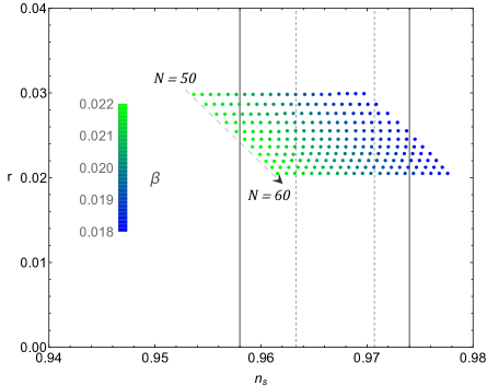
Figure 1: A plot of the $n_{s}-r$ plane, for $\alpha=10^{7}$, $\lambda=10^{-13}$, $\xi=10^{-6}$ and varying values of $\beta\in\left\{0.018,0.022\right\}$. The dashed and solid lines represent the $1\sigma$ and $2\sigma$ allowed range of the $n_{s}$, respectively, while the whole of the presented parameter space is allowed for $r$ ($r<0.06$). Once again, as $|\beta|$ increases, the spectral tilt $n_{s}$ decreases, while the effect on the tensor-to-scalar ratio $r$ is minimal, $r_{N=50}=3\times 10^{-2}$ and $r_{N=60}=2\times 10^{-2}$.

The values of the parameters, $\alpha=10^{7}$, $\lambda=10^{-13}$ and $\xi=10^{-6}$ are chosen such that they reproduce the observable value of the power spectrum in (3.7). As expected the model can provide an appropriate amount of inflation in the large field domain with relevant results for the inflationary observables. Also, we find that the slow-roll parameters indeed assume small values, in this case as well, i.e. $\epsilon_{1}\lesssim 10^{-2}$ and $|\epsilon_{4}|\sim 10^{-2}$.

The numerical value of the parameter $C_{s}^{2}$, both in the case of minimal and non-minimal coupling, is $C_{s}^{2}\simeq 0.34$. As expected we obtain values of $C_{s}^{2}<1$, while also avoiding instabilities associated with $C_{s}^{2}<0$. This value holds true throughout the stages of inflation, however, when $\phi\sim M_{P}$, the parameter tends rapidly to $C_{s}^{2}\sim 1$.

5 Summary

In the present article we investigated the inflationary/phenomenological predictions of a scalar field coupled to quadratic gravity in the framework of the Palatini formulation. The resulting Einstein-frame generalized $k$-inflation effective theory was analyzed assuming that a constant-roll condition $\ddot{\phi}\!\sim\!\beta H\dot{\phi}$ holds. The equations of motion were derived, as well as the general expressions for the slow-roll parameters and observational indices. We focused on a quartic self-interaction potential, a case of particular appeal modelling Higgs inflation, considering both the cases of minimal and non-minimal coupling of the inflaton to gravity. The results show a significant contribution from the additional kinetic terms, in contrast to the slow-roll analysis of the same model. For an appropriate range of the model parameters, with inflationary dynamics taking place in the large field domain, we obtained values for the inflationary observables, namely the primordial tilt $n_{s}$, the tensor-to-scalar ratio $r$ and the power spectrum, in the general range allowed by observations both in the case of the minimal coupling as well as the case of non-minimal coupling of the scalar to gravity. Contrary to the slow-roll analysis of the same model, where these results required an unusually large amount of $e$-folds, in the present case of constant-roll inflation the appropriate amount of $e$-fold was retained.

References

- [1] A. A. Starobinsky, A New Type of Isotropic Cosmological Models Without Singularity, Phys. Lett. 91B (1980) 99–102.
- [2] A. H. Guth, The Inflationary Universe: A Possible Solution to the Horizon and Flatness Problems, Phys. Rev. D23 (1981) 347–356.
- [3] K. Sato, First Order Phase Transition of a Vacuum and Expansion of the Universe, Mon. Not. Roy. Astron. Soc. 195 (1981) 467–479.
- [4] A. D. Linde, A New Inflationary Universe Scenario: A Possible Solution of the Horizon, Flatness, Homogeneity, Isotropy and Primordial Monopole Problems, Phys. Lett. 108B (1982) 389–393.
- [5] A. Albrecht and P. J. Steinhardt, Cosmology for Grand Unified Theories with Radiatively Induced Symmetry Breaking, Phys. Rev. Lett. 48 (1982) 1220–1223.
- [6] A. D. Linde, Chaotic Inflation, Phys. Lett. 129B (1983) 177–181.
- [7] D. H. Lyth and A. Riotto, Particle physics models of inflation and the cosmological density perturbation, Physics Reports 314 (1999), no. 1 1–146.
- [8] A. A. Starobinsky, Spectrum of relict gravitational radiation and the early state of the universe, JETP Lett. 30 (1979) 682–685. [Pisma Zh. Eksp. Teor. Fiz.30,719(1979); ,767(1979)].
- [9] V. F. Mukhanov and G. V. Chibisov, Quantum Fluctuations and a Nonsingular Universe, JETP Lett. 33 (1981) 532–535. [Pisma Zh. Eksp. Teor. Fiz.33,549(1981)].
- [10] S. W. Hawking, The Development of Irregularities in a Single Bubble Inflationary Universe, Phys. Lett. 115B (1982) 295.
- [11] S. W. Hawking and I. G. Moss, Fluctuations in the Inflationary Universe, Nucl. Phys. B224 (1983) 180.
- [12] A. A. Starobinsky, Dynamics of Phase Transition in the New Inflationary Universe Scenario and Generation of Perturbations, Phys. Lett. 117B (1982) 175–178.
- [13] A. H. Guth and S. Y. Pi, Fluctuations in the New Inflationary Universe, Phys. Rev. Lett. 49 (1982) 1110–1113.
- [14] Planck Collaboration, Y. Akrami et al., Planck 2018 results. X. Constraints on inflation, arXiv:1807.06211.
- [15] BICEP2, Keck Array Collaboration, P. A. R. Ade et al., BICEP2 / Keck Array x: Constraints on Primordial Gravitational Waves using Planck, WMAP, and New BICEP2/Keck Observations through the 2015 Season, Phys. Rev. Lett. 121 (2018) 221301, [arXiv:1810.05216].
- [16] A. De Felice and S. Tsujikawa, f(R) theories, Living Rev. Rel. 13 (2010) 3, [arXiv:1002.4928].
- [17] T. P. Sotiriou and V. Faraoni, f(R) Theories Of Gravity, Rev. Mod. Phys. 82 (2010) 451–497, [arXiv:0805.1726].
- [18] S. Capozziello and M. De Laurentis, Extended Theories of Gravity, Phys. Rept. 509 (2011) 167–321, [arXiv:1108.6266].
- [19] T. Clifton, P. G. Ferreira, A. Padilla, and C. Skordis, Modified Gravity and Cosmology, Phys. Rept. 513 (2012) 1–189, [arXiv:1106.2476].
- [20] S. D. Odintsov and V. K. Oikonomou, Inflationary -attractors from gravity, Phys. Rev. D94 (2016), no. 12 124026, [arXiv:1612.01126].
- [21] A. Palatini, Deduzione invariantiva delle equazioni gravitazionali dal principio di hamilton, Rendiconti del Circolo Matematico di Palermo (1884-1940) 43 (Dec, 1919) 203–212.
- [22] F. Bauer and D. A. Demir, Inflation with Non-Minimal Coupling: Metric versus Palatini Formulations, Phys. Lett. B665 (2008) 222–226, [arXiv:0803.2664].
- [23] M. Borunda, B. Janssen, and M. Bastero-Gil, Palatini versus metric formulation in higher curvature gravity, JCAP 0811 (2008) 008, [arXiv:0804.4440].
- [24] F. Bauer and D. A. Demir, Higgs-Palatini Inflation and Unitarity, Phys. Lett. B698 (2011) 425–429, [arXiv:1012.2900].
- [25] N. Tamanini and C. R. Contaldi, Inflationary Perturbations in Palatini Generalised Gravity, Phys. Rev. D83 (2011) 044018, [arXiv:1010.0689].
- [26] K. Enqvist, T. Koivisto, and G. Rigopoulos, Non-metric chaotic inflation, JCAP 1205 (2012) 023, [arXiv:1107.3739].
- [27] A. Borowiec, M. Kamionka, A. Kurek, and M. Szydlowski, Cosmic acceleration from modified gravity with Palatini formalism, JCAP 1202 (2012) 027, [arXiv:1109.3420].
- [28] A. Racioppi, Coleman-Weinberg linear inflation: metric vs. Palatini formulation, JCAP 1712 (2017), no. 12 041, [arXiv:1710.04853].
- [29] S. Rasanen and P. Wahlman, Higgs inflation with loop corrections in the Palatini formulation, JCAP 1711 (2017), no. 11 047, [arXiv:1709.07853].
- [30] C. Fu, P. Wu, and H. Yu, Inflationary dynamics and preheating of the nonminimally coupled inflaton field in the metric and Palatini formalisms, Phys. Rev. D96 (2017), no. 10 103542, [arXiv:1801.04089].
- [31] A. Stachowski, M. Szydłowski, and A. Borowiec, Starobinsky cosmological model in Palatini formalism, Eur. Phys. J. C77 (2017), no. 6 406, [arXiv:1608.03196].
- [32] H. Azri and D. Demir, Affine Inflation, Phys. Rev. D95 (2017), no. 12 124007, [arXiv:1705.05822].
- [33] V.-M. Enckell, K. Enqvist, S. Rasanen, and E. Tomberg, Higgs inflation at the hilltop, JCAP 1806 (2018), no. 06 005, [arXiv:1802.09299].
- [34] V.-M. Enckell, K. Enqvist, S. Rasanen, and L.-P. Wahlman, Inflation with term in the Palatini formalism, arXiv:1810.05536.
- [35] L. Järv, A. Racioppi, and T. Tenkanen, Palatini side of inflationary attractors, Phys. Rev. D97 (2018), no. 8 083513, [arXiv:1712.08471].
- [36] S. Rasanen, Higgs inflation in the Palatini formulation with kinetic terms for the metric, arXiv:1811.09514.
- [37] I. Antoniadis, A. Karam, A. Lykkas, and K. Tamvakis, Palatini inflation in models with an term, JCAP 1811 (2018), no. 11 028, [arXiv:1810.10418].
- [38] S. Rasanen and E. Tomberg, Planck scale black hole dark matter from Higgs inflation, arXiv:1810.12608.
- [39] I. Antoniadis, A. Karam, A. Lykkas, T. Pappas, and K. Tamvakis, Rescuing Quartic and Natural Inflation in the Palatini Formalism, JCAP 1903 (2019) 005, [arXiv:1812.00847].
- [40] A. Racioppi, Non-Minimal (Self-)Running Inflation: Metric vs. Palatini Formulation, arXiv:1912.10038.
- [41] K. Shimada, K. Aoki, and K.-i. Maeda, Metric-affine Gravity and Inflation, Phys. Rev. D99 (2019), no. 10 104020, [arXiv:1812.03420].
- [42] R. Jinno, K. Kaneta, K.-y. Oda, and S. C. Park, Hillclimbing inflation in metric and Palatini formulations, Phys. Lett. B791 (2019) 396–402, [arXiv:1812.11077].
- [43] T. Tenkanen, Minimal Higgs inflation with an term in Palatini gravity, Phys. Rev. D99 (2019), no. 6 063528, [arXiv:1901.01794].
- [44] J. Rubio and E. S. Tomberg, Preheating in Palatini Higgs inflation, JCAP 1904 (2019), no. 04 021, [arXiv:1902.10148].
- [45] I. D. Gialamas and A. B. Lahanas, Reheating in Palatini inflationary models, arXiv:1911.11513.
- [46] T. Tenkanen, Tracing the high energy theory of gravity: an introduction to Palatini inflation, arXiv:2001.10135.
- [47] M. Shaposhnikov, A. Shkerin, and S. Zell, Standard Model Meets Gravity: Electroweak Symmetry Breaking and Inflation, arXiv:2001.09088.
- [48] T. Tenkanen and E. Tomberg, Initial conditions for plateau inflation, arXiv:2002.02420.
- [49] M. Shaposhnikov, A. Shkerin, and S. Zell, Quantum Effects in Palatini Higgs Inflation, arXiv:2002.07105.
- [50] A. Lloyd-Stubbs and J. McDonald, Sub-Planckian Inflation in the Palatini Formulation of Gravity with an term, arXiv:2002.08324.
- [51] C. Armendariz-Picon, T. Damour, and V. F. Mukhanov, k - inflation, Phys. Lett. B458 (1999) 209–218, [hep-th/9904075].
- [52] T. Chiba, T. Okabe, and M. Yamaguchi, Kinetically driven quintessence, Phys. Rev. D62 (2000) 023511, [astro-ph/9912463].
- [53] C. Armendariz-Picon, V. F. Mukhanov, and P. J. Steinhardt, A Dynamical solution to the problem of a small cosmological constant and late time cosmic acceleration, Phys. Rev. Lett. 85 (2000) 4438–4441, [astro-ph/0004134].
- [54] C. Armendariz-Picon, V. F. Mukhanov, and P. J. Steinhardt, Essentials of k essence, Phys. Rev. D63 (2001) 103510, [astro-ph/0006373].
- [55] T. Chiba, Tracking K-essence, Phys. Rev. D66 (2002) 063514, [astro-ph/0206298].
- [56] M. Malquarti, E. J. Copeland, A. R. Liddle, and M. Trodden, A New view of k-essence, Phys. Rev. D67 (2003) 123503, [astro-ph/0302279].
- [57] M. Malquarti, E. J. Copeland, and A. R. Liddle, K-essence and the coincidence problem, Phys. Rev. D68 (2003) 023512, [astro-ph/0304277].
- [58] L. P. Chimento and A. Feinstein, Power - law expansion in k-essence cosmology, Mod. Phys. Lett. A19 (2004) 761–768, [astro-ph/0305007].
- [59] L. P. Chimento, Extended tachyon field, Chaplygin gas and solvable k-essence cosmologies, Phys. Rev. D69 (2004) 123517, [astro-ph/0311613].
- [60] R. J. Scherrer, Purely kinetic k-essence as unified dark matter, Phys. Rev. Lett. 93 (2004) 011301, [astro-ph/0402316].
- [61] J. M. Aguirregabiria, L. P. Chimento, and R. Lazkoz, Phantom k-essence cosmologies, Phys. Rev. D70 (2004) 023509, [astro-ph/0403157].
- [62] C. Armendariz-Picon and E. A. Lim, Haloes of k-essence, JCAP 0508 (2005) 007, [astro-ph/0505207].
- [63] L. R. Abramo and N. Pinto-Neto, On the stability of phantom k-essence theories, Phys. Rev. D73 (2006) 063522, [astro-ph/0511562].
- [64] A. D. Rendall, Dynamics of k-essence, Class. Quant. Grav. 23 (2006) 1557–1570, [gr-qc/0511158].
- [65] J.-P. Bruneton, On causality and superluminal behavior in classical field theories: Applications to k-essence theories and MOND-like theories of gravity, Phys. Rev. D75 (2007) 085013, [gr-qc/0607055].
- [66] R. de Putter and E. V. Linder, Kinetic k-essence and Quintessence, Astropart. Phys. 28 (2007) 263–272, [arXiv:0705.0400].
- [67] E. Babichev, V. Mukhanov, and A. Vikman, k-Essence, superluminal propagation, causality and emergent geometry, JHEP 02 (2008) 101, [arXiv:0708.0561].
- [68] J. Matsumoto and S. Nojiri, Reconstruction of k-essence model, Phys. Lett. B687 (2010) 236–242, [arXiv:1001.0220].
- [69] C. Deffayet, X. Gao, D. A. Steer, and G. Zahariade, From k-essence to generalised Galileons, Phys. Rev. D84 (2011) 064039, [arXiv:1103.3260].
- [70] S. Unnikrishnan, V. Sahni, and A. Toporensky, Refining inflation using non-canonical scalars, JCAP 1208 (2012) 018, [arXiv:1205.0786].
- [71] S. Li and A. R. Liddle, Observational constraints on K-inflation models, JCAP 1210 (2012) 011, [arXiv:1204.6214].
- [72] H. Motohashi, A. A. Starobinsky, and J. Yokoyama, Inflation with a constant rate of roll, JCAP 1509 (2015), no. 09 018, [arXiv:1411.5021].
- [73] H. Motohashi and A. A. Starobinsky, Constant-roll inflation: confrontation with recent observational data, Europhys. Lett. 117 (2017), no. 3 39001, [arXiv:1702.05847].
- [74] S. D. Odintsov and V. K. Oikonomou, Inflationary Dynamics with a Smooth Slow-Roll to Constant-Roll Era Transition, JCAP 1704 (2017), no. 04 041, [arXiv:1703.02853].
- [75] S. D. Odintsov and V. K. Oikonomou, Inflation with a Smooth Constant-Roll to Constant-Roll Era Transition, Phys. Rev. D96 (2017), no. 2 024029, [arXiv:1704.02931].
- [76] S. Nojiri, S. D. Odintsov, and V. K. Oikonomou, Constant-roll Inflation in Gravity, Class. Quant. Grav. 34 (2017), no. 24 245012, [arXiv:1704.05945].
- [77] H. Motohashi and A. A. Starobinsky, constant-roll inflation, Eur. Phys. J. C77 (2017), no. 8 538, [arXiv:1704.08188].
- [78] Q. Gao, Reconstruction of constant slow-roll inflation, Sci. China Phys. Mech. Astron. 60 (2017), no. 9 090411, [arXiv:1704.08559].
- [79] V. K. Oikonomou, Reheating in Constant-roll Gravity, Mod. Phys. Lett. A32 (2017), no. 33 1750172, [arXiv:1706.00507].
- [80] S. D. Odintsov, V. K. Oikonomou, and L. Sebastiani, Unification of Constant-roll Inflation and Dark Energy with Logarithmic -corrected and Exponential Gravity, Nucl. Phys. B923 (2017) 608–632, [arXiv:1708.08346].
- [81] V. K. Oikonomou, A Smooth Constant-Roll to a Slow-Roll Modular Inflation Transition, Int. J. Mod. Phys. D27 (2017), no. 02 1850009, [arXiv:1709.02986].
- [82] F. Cicciarella, J. Mabillard, and M. Pieroni, New perspectives on constant-roll inflation, JCAP 1801 (2018), no. 01 024, [arXiv:1709.03527].
- [83] L. Anguelova, P. Suranyi, and L. C. R. Wijewardhana, Systematics of Constant Roll Inflation, JCAP 1802 (2017), no. 02 004, [arXiv:1710.06989].
- [84] A. Karam, L. Marzola, T. Pappas, A. Racioppi, and K. Tamvakis, Constant-Roll (Quasi-)Linear Inflation, JCAP 1805 (2018), no. 05 011, [arXiv:1711.09861].
- [85] Z. Yi and Y. Gong, On the constant-roll inflation, arXiv:1712.07478.
- [86] Q. Gao, Y. Gong, and Z. Yi, On the constant-roll inflation with large and small , Universe 5 (2019), no. 11 215, [arXiv:1901.04646].
- [87] S. D. Odintsov and V. K. Oikonomou, Constant-roll -Inflation Dynamics, Class. Quant. Grav. 37 (2020), no. 2 025003, [arXiv:1912.00475].
- [88] F. L. Bezrukov and M. Shaposhnikov, The Standard Model Higgs boson as the inflaton, Phys. Lett. B659 (2008) 703–706, [arXiv:0710.3755].
- [89] A. De Simone, M. P. Hertzberg, and F. Wilczek, Running Inflation in the Standard Model, Phys. Lett. B678 (2009) 1–8, [arXiv:0812.4946].
- [90] F. L. Bezrukov, A. Magnin, and M. Shaposhnikov, Standard Model Higgs boson mass from inflation, Phys. Lett. B675 (2009) 88–92, [arXiv:0812.4950].
- [91] J. L. F. Barbon and J. R. Espinosa, On the Naturalness of Higgs Inflation, Phys. Rev. D79 (2009) 081302, [arXiv:0903.0355].
- [92] A. O. Barvinsky, A. Yu. Kamenshchik, C. Kiefer, A. A. Starobinsky, and C. Steinwachs, Asymptotic freedom in inflationary cosmology with a non-minimally coupled Higgs field, JCAP 0912 (2009) 003, [arXiv:0904.1698].
- [93] R. N. Lerner and J. McDonald, A Unitarity-Conserving Higgs Inflation Model, Phys. Rev. D82 (2010) 103525, [arXiv:1005.2978].
- [94] F. Bezrukov, A. Magnin, M. Shaposhnikov, and S. Sibiryakov, Higgs inflation: consistency and generalisations, JHEP 01 (2011) 016, [arXiv:1008.5157].
- [95] K. Kamada, T. Kobayashi, T. Takahashi, M. Yamaguchi, and J. Yokoyama, Generalized Higgs inflation, Phys. Rev. D86 (2012) 023504, [arXiv:1203.4059].
- [96] F. Bezrukov, The Higgs field as an inflaton, Class. Quant. Grav. 30 (2013) 214001, [arXiv:1307.0708].
- [97] F. Bezrukov and M. Shaposhnikov, Higgs inflation at the critical point, Phys. Lett. B734 (2014) 249–254, [arXiv:1403.6078].
- [98] K. Allison, Higgs xi-inflation for the 125-126 GeV Higgs: a two-loop analysis, JHEP 02 (2014) 040, [arXiv:1306.6931].
- [99] Y. Hamada, H. Kawai, and K.-y. Oda, Minimal Higgs inflation, PTEP 2014 (2014) 023B02, [arXiv:1308.6651].
- [100] D. P. George, S. Mooij, and M. Postma, Quantum corrections in Higgs inflation: the real scalar case, JCAP 1402 (2014) 024, [arXiv:1310.2157].
- [101] A. Salvio and A. Mazumdar, Classical and Quantum Initial Conditions for Higgs Inflation, Phys. Lett. B750 (2015) 194–200, [arXiv:1506.07520].
- [102] Y. Hamada, H. Kawai, K.-y. Oda, and S. C. Park, Higgs inflation from Standard Model criticality, Phys. Rev. D91 (2015) 053008, [arXiv:1408.4864].
- [103] X. Calmet and I. Kuntz, Higgs Starobinsky Inflation, Eur. Phys. J. C76 (2016), no. 5 289, [arXiv:1605.02236].
- [104] M. Artymowski, Z. Lalak, and M. Lewicki, Saddle point inflation from higher order corrections to Higgs/Starobinsky inflation, Phys. Rev. D93 (2016), no. 4 043514, [arXiv:1509.00031].
- [105] J. Rubio, Higgs inflation, arXiv:1807.02376.
- [106] H. Noh and J.-c. Hwang, Inflationary spectra in generalized gravity: Unified forms, Phys. Lett. B515 (2001) 231–237, [astro-ph/0107069].
- [107] J.-c. Hwang and H. Noh, Cosmological perturbations in a generalized gravity including tachyonic condensation, Phys. Rev. D66 (2002) 084009, [hep-th/0206100].
- [108] J.-c. Hwang and H. Noh, Classical evolution and quantum generation in generalized gravity theories including string corrections and tachyon: Unified analyses, Phys. Rev. D71 (2005) 063536, [gr-qc/0412126].
- [109] Y.-C. Wang and T. Wang, Primordial perturbations generated by Higgs field and operator, Phys. Rev. D96 (2017), no. 12 123506, [arXiv:1701.06636].
- [110] Y. Ema, Higgs Scalaron Mixed Inflation, Phys. Lett. B770 (2017) 403–411, [arXiv:1701.07665].
- [111] M. He, A. A. Starobinsky, and J. Yokoyama, Inflation in the mixed Higgs- model, JCAP 1805 (2018) 064, [arXiv:1804.00409].
- [112] V.-M. Enckell, K. Enqvist, S. Rasanen, and L.-P. Wahlman, Higgs- inflation - full slow-roll study at tree-level, arXiv:1812.08754. [JCAP2001,no.01,041(2020)].