Localized waves in the nonlinear rhombic waveguide array

Abstract

Solitary electromagnetic waves propagating along the waveguides forming a rhombic one-dimensional lattice are considered. Two waveguides that are part of the unit cell are assumed to be made of an optical linear material, while the third waveguide from the same array is composed of material with the cubic nonlinearity. The equations of the coupled waves spreading in each waveguide are solved under some approximation. These solutions represent the breather like solitary waves, which are akin to three component soliton.

1 Introduction

The first demonstration of the discrete photonic device was presented in [1]. It was shown that the array of a closely spaced waveguides acts as the Bragg grating. In [2, 3, 4] the anomalous refraction and diffraction in a discrete photonic system produced from an array of coupled waveguides was experimentally studied. In waveguide arrays with linearly varying propagation constants the optical Bloch oscillations observed [5] The existence of localized modes with equidistant wave-number spacing that do not undergo diffraction is analytically proved [5, 6].

Over the last ten years the periodic one-dimensional or two-dimensional lattices of waveguides whose coupling is due to disturbed total internal reflection are the popular models of the discrete photonics [7, 8, 9].

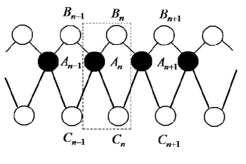
Figure 1: Binary rhombic array of waveguides. The unit cell of a one-dimensional array is marked with a rectangle.

If the unit cell of the waveguide lattice contains more than two ”atoms”  the photon spectrum has several branches. There are conditions where one or more branches have zero curvature in a space of quasi-pulses. The expression for the light wave frequency does not depend on the transverse wave numbers. The corresponding spectral bands are called flat bands. The fields attributed to a superposition of modes from the flat band remain localized on the waveguide array. In other words, theses fields correspond to beams, which are free of discrete diffraction.

A rhombic waveguide array (Fig.1) is the example of the discrete medium where the photon spectrum has one flat band and two usual bands [10, 11]. In the linear case existence of the localized flat band modes in the rhombic waveguide array was experimentally demonstrate [12, 13]. Recent review devoted to the optical system with a flat band is [14]. In general case in a nonlinear rhombic waveguide array the modes of the all band are stirred due to waveguide material nonlinearity. The diffraction is restored [15, 16].

In this paper the binary nonlinear rhombic waveguide array will be considered. Unit cell contains one nonlinear waveguide and two linear ones. In [17] the waves localized on the axis of waveguides was considered. Oppositely, here the waves will be assumed localized on transverse direction but along the waveguide direction waves are not localized.

2 Basic equations

Let the $A_{n}$, $B_{n}$ and $C_{n}$ be the normalized field amplitudes in a waveguide of the $n$th unit cell (Fig.1). Evolution of theses values is governed by the following system of equations [17]

$$i(\partial_{\tau}+\partial_{\zeta})A_{n}+(B_{n}+B_{n-1})+\gamma(C_{n}+C_{n-1})+\mu|A_{n}|^{2}A_{n}=0,$$ (1)

$$i(\partial_{\tau}+\partial_{\zeta})B_{n}+(A_{n}+A_{n+1})=0,$$ (2)

$$i(\partial_{\tau}+\partial_{\zeta})C_{n}+\gamma(A_{n}+A_{n+1})=0,$$ (3)

where $\zeta$ is a dimensionless coordinate measured in units of coupling length between the waveguides of types $\mathrm{A}$ and $\mathrm{B}$, $\tau$ is dimensionless time. Here the symbol $\partial_{s}$ is used instead of $\partial/\partial s$. Parameter $\gamma$ is coupling constant ratio between waveguides of types $\mathrm{A}$ and $\mathrm{C}$. Waveguides of types $\mathrm{B}$ and $\mathrm{C}$ are made of an optical linear material, while the waveguide of type $\mathrm{A}$ is composed of material with the cubic nonlinearity. Parameter $\mu$ considers the nonlinear properties of waveguides of type $\mathrm{A}$.

If one introduce new variables $F_{n}=B_{n}+\gamma C_{n}$ and $G_{n}=B_{n}-\gamma C_{n}$, then the system of equations (1)–(3) will reads

$$i(\partial_{\tau}+\partial_{\zeta})A_{n}+(F_{n}+F_{n-1})+\mu|A_{n}|^{2}A_{n}=0,$$ (4)

$$i(\partial_{\tau}+\partial_{\zeta})F_{n}+(1+\gamma^{2})(A_{n}+A_{n+1})=0,$$ (5)

$$i(\partial_{\tau}+\partial_{\zeta})G_{n}+(1-\gamma^{2})(A_{n}+A_{n+1})=0.$$ (6)

It should be remarked that $F_{n}$ and $A_{n}$ are coupled to one another though equations (4) and (5). The amplitudes $G_{n}$ are determined by only $A_{n}+A_{n+1}$.

3 Continuum approximation

Let us $A_{n}=(-1)^{n}\tilde{A}_{n}$ and $F_{n}=(-1)^{n}\tilde{F}_{n}$ where $\tilde{A}_{n}$ and $\tilde{F}_{n}$ are the slowly varying variables as the function of $n$. The second proposition is

$$\tilde{A}_{n}(\tau,\zeta)=a_{n}\exp[i\beta(\zeta+\tau)],\quad\tilde{F}_{n}(\tau,\zeta)=f_{n}\exp[i\beta(\zeta+\tau)].$$

Then the system of equations (4) and (5) reduces to

$$-\beta a_{n}+(f_{n}-f_{n-1})+\mu|a_{n}|^{2}a_{n}=0,$$ (7)

$$-\beta f_{n}+(1+\gamma^{2})(a_{n}-a_{n+1})=0,$$ (8)

These equations are not contain the imaginary unit, hence the variables $a_{n}$ and $f_{n}$ are real ones. Elimination $f_{n}$ results in the equation for $a_{n}$:

$$\beta^{2}a_{n}+(1+\gamma^{2})(a_{n-1}+a_{n-1}-2a_{n})-\beta\mu a_{n}^{3}=0.$$ (9)

Now the continuum approximation will be done. Variable $a_{n}$ will be considered as the function of $\xi=n\delta l$ ($\delta l$ is the lattice parameter). If the $a_{n}$ varies only slightly over several $\delta l$, then the following approximation

$$a_{n\pm 1}\approx a\pm\frac{\partial a}{\partial\xi}+\frac{1}{2}\frac{\partial^{2}a}{\partial\xi^{2}},$$

can be assumed. In this approximation equation (9) is reduced to

$$\beta^{2}a+(1+\gamma^{2})\frac{\partial^{2}a}{\partial\xi^{2}}-\beta\mu a^{3}=0.$$ (10)

The amplitude $f$ is

$$\beta f=-(1+\gamma^{2})\frac{\partial a}{\partial\xi}.$$

Solution of the equation (10) can be found by standard way. Under condition that $a(\xi)\to 0$ at $|\xi|\to\infty$, solution of the (10) takes the following form

$$a(\xi)=\sqrt{\frac{2\beta}{\mu}}\mathrm{sech}\left(\frac{\beta\xi}{\sqrt{1+\gamma^{2}}}\right).$$ (11)

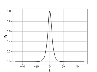
Figure 2: Slowly varying envelope $a(\xi)$ for localized wave in the waveguides of type $\mathrm{A}$.

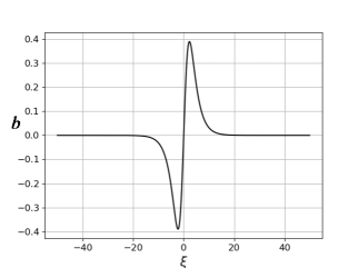
Figure 3: Slowly varying envelope $b(\xi)$ for localized wave in the waveguides of type $\mathrm{B}$.

Taking into account the relationship between $G_{n}$, $F_{n}$, $B_{n}$ and $A_{n}$ one can find the following expressions

$$A_{n}(\tau,\zeta)=(-1)^{n}a(\xi)\exp[i\beta(\zeta+\tau)],$$

$$B_{n}(\tau,\zeta)=(-1)^{n}b(\xi)\exp[i\beta(\zeta+\tau)],$$ (12)

$$C_{n}(\tau,\zeta)=(-1)^{n}c(\xi)\exp[i\beta(\zeta+\tau)],$$

where $\xi=n\delta l$, $a(\xi)$ is defined by equation (11), $b(\xi)$ and $c(\xi)$ are equal to

$$b(\xi)=\frac{1}{\sqrt{1+\gamma^{2}}}\sqrt{\frac{2\beta}{\mu}}\tanh\left(\frac{\beta\xi}{\sqrt{1+\gamma^{2}}}\right)\mathrm{sech}\left(\frac{\beta\xi}{\sqrt{1+\gamma^{2}}}\right),$$ (13)

$$c(\xi)=\frac{\gamma}{\sqrt{1+\gamma^{2}}}\sqrt{\frac{2\beta}{\mu}}\tanh\left(\frac{\beta\xi}{\sqrt{1+\gamma^{2}}}\right)\mathrm{sech}\left(\frac{\beta\xi}{\sqrt{1+\gamma^{2}}}\right).$$ (14)

Slowly varying envelopes of the electric field distributions (12) are presented on Fig.3 and Fig.3. These plots was calculated by using (11) and (13) at $\beta=0.5$, $\gamma=0.8$ and $\mu=1$. There only $a(\xi)$ and $b(\xi)$ are presented as the difference between $c(\xi)$ and $b(\xi)$ is trivial.

4 Conclusions

The waves propagating along the axis of a periodic one-dimensional binary rhombic array formed by waveguides of different types are investigated. For the system of coupled mode equations approximate solution was found in the case of the cubic nonlinearity of a central waveguide line (Fig. 1). Two other lines were composed of waveguides made of linear material. The obtained solution describes a nonlinear solitary wave, which is akin to three component soliton.

It should be remarked that the electric fields in waveguides of $\mathrm{A}$ and $\mathrm{B}$ types are identical in phase. Localization of the fields is due to a dynamical reason. We not consider the phenomenon of the flat band, where localization stems from the interference of the electromagnetic fields [14, 18, 19].

References

References

- [1] Somekh S, Garmire E, Yariv A, et al. 1973 Appl.Phys.Lett. 22 46-7
- [2] Pertsch T, Zentgraf T, Peschel U, et al 2002 Phys. Rev. Lett. 88 093901
- [3] Staron G, Weinert-Raczka E, and Urban P 2005 Opto-Electronics Review 13 93-102
- [4] Röpke U, Bartelt H, and Unger S. 2011 Appl. Phys. B. 104 481-6
- [5] Peschel U, Pertsch T, Lederer F 1998 Opt. Lett. 23 1701 03
- [6] Szameit A, Pertsch T, Nolte S, et al. 2007 J. Opt. Soc. Amer. 24 2632-39
- [7] Longhi S 2009 Laser & Photonics Reviews 3 243 61
- [8] Szameit A and Nolte S 2010 J. Phys.B: Atomic, Molecular and Optical Physics 43 163001
- [9] Maimistov A I 2016 Nonlinear Phenomena in Complex Systems 19 358-67
- [10] Flach S, Leykam D, Bodyfelt J D, Matthies P, and Desyatnikov A S 2014 Europhys. Lett. 105 30001
- [11] Longhi St, 2014 Opt. Lett. 39 5892-95
- [12] Mukherjee S and Thomson R R 2015 Opt. Lett. 40 5443-46
- [13] Mukherjee S and Thomson R R 2017 Opt. Lett. 42 2243-46
- [14] Leykam D, Andreanov A, and Flach S 2018 Advances in Physics X 3 1473052
- [15] Zegadlo K, Dror N, Hung N V, Trippenbach M, and A. Malomed B A 2017 Phys.Rev. E 96 012204
- [16] Maimistov A I 2017 J. Opt. 19 045502
- [17] Maimistov A I 2018 Bulletin of the Russian Academy of Sciences: Physics 82 1363-66
- [18] Maimistov A I and Patrikeev V A 2016 J. Phys.: Conf. Series 737 012008
- [19] Gligoric G, Maluckov A, Hadzievski Lj, Flach S and Malomed B A 2016 Phys. Rev. 94 144302