Fast Indexes for Gapped Pattern Matching

Abstract

We describe indexes for searching large data sets for variable-length-gapped (VLG) patterns. VLG patterns are composed of two or more subpatterns, between each adjacent pair of which is a gap-constraint specifying upper and lower bounds on the distance allowed between subpatterns. VLG patterns have numerous applications in computational biology (motif search), information retrieval (e.g., for language models, snippet generation, machine translation) and capture a useful subclass of the regular expressions commonly used in practice for searching source code. Our best approach provides search speeds several times faster than prior art across a broad range of patterns and texts.

1 Introduction

In the classic pattern matching problem, we are given a string P (the pattern or query) and asked to report all the positions where it occures in another (longer) string T (the text). This problem has been very heavily studied and has applications throughout computer science.

In this paper we consider a variant on the classic pattern matching problem, called variable length gap (VLG) pattern matching. In VLG matching, the query P is not a single string but is composed of $k\geq 2$ strings (subpatterns) that must occur in order in the text. Between each subpattern, a number of characters may be allowed to occur, an upper and lower bound on which is specified as part of the query. Formally, our problem is as follows.

Definition 1 (Variable Length Gap (VLG) Pattern Matching [4])

Let T be a string of $n$ symbols drawn from alphabet $\Sigma$ and P be a pattern consisting of $k\geq 2$ subpatterns (i.e. strings) $p_{0},\ldots,p_{k-1}$, each consisting of symbols also drawn from $\Sigma$, and having lengths $m_{0},\ldots,m_{k-1}$, and $k-1$ gap constraints $C_{0},\ldots,C_{k-2}$, such that $C_{i}=\langle\delta_{i},\Delta_{i}\rangle$ with $0\leq\delta_{i}\leq\Delta_{i}<n$ specifies the smallest ($\delta_{i}$) and largest ($\Delta_{i}$) allowable distance between a match of $p_{i}$ and $p_{i+1}$ in T. Find all matches — reported as $k$-tuples $i_{0},\ldots,i_{k-1}$ where $i_{j}$ is the starting position for subpattern $p_{j}$ in T — such that all gap constraints are satisfied.

In computational biology, VLG matching is used in the discovery of and search for motifs — i.e. conserved features — in sets of DNA and protein sequences (see, e.g., [18, 20]). For example, the following is a protein motif from the rice genome (see [18]) expressed as a VLG pattern:

MT[115, 136]MTNTAYGG[121, 151]GTNGAYGAY.

A similar motif concept in music information retrieval means VLG matching also finds applications in mining and searching for characteristic melodies [7] and other musical structures [8, 9] in sequences of musical notes expressed in chromatic or diatonic notation. Bader et al. [1] point out several more applications of VLG matching in information retrieval and related fields such as natural language processing (NLP) and machine translation. For example, Metzler and Croft [17] define a language model in which query terms occuring within as certain window of each other must be found (in NLP, such terms are said to be colocated). Locating tight windows of a document containing the set of words contained in a search engine query is the problem of query-biased snippet generation [22]. In machine translation, VLG matching is used to derive rule sets from text collections to boost effectiveness of automated translation systems [15].

VLG matching has a big parameter space and it is easy to think of pathological combinations of pattern and text that lead to an exponential number of matches. Fortunately, however, in practice the problem gets naturally constrained in important ways. The gap constraints are always bound the length of documents under consideration, which in the case of source code or web pages means that usually $\delta_{i}$ and $\Delta_{i}$ (and so their difference) are in (at most) the tens-of-kilobytes range. In genomics and proteomics maximum gaps tend to be around 100 characters or so (see, e.g., [18, 20]).

Because of the interesting and useful applications outlined above, VLG matching has received a great deal of attention in the past 20 years. The vast majority of previous work deals with the online version of the problem in which both the pattern P and the text T are previously unseen and cannot be preprocessed [2, 4, 5, 9, 12, 18, 21]. Our concern in this paper is the offline version of the problem, where T is known in advance and can be preprocessed and an index structure built and stored to later support fast search for previously unseen VLG patterns (the stream of which is assumed to be large, practically infinite). Almost all work on the offline problem is of theoretical interest [14, 3]. The exception is the recent work of Bader, Gog, and Petri [1], who develop methods for the offline setting that use a combination of suffix arrays [16] and wavelet trees [11, 19]. Bader et al. show that their index is an order of magnitude faster at VLG matching than are online methods, and several times faster than $q$-gram-based indexes, the likes of which were behind Google Code Search [6].

Contribution.

Our main contribution in the paper is to show that in practice, on a broad range of inputs typical in real applications of VLG matching, simple algorithms based on intersecting ranges of the suffix array corresponding to subpattern occurrences can be made very fast in practice, and comfortably outperform state-of-the-art methods based on wavelet trees.

We emphasise that none of our new approaches are particularly exotic. They are, however, very fast, and so represent non-trivial baselines by which future (possibly more exotic) indexes for VLG pattern matching and related problems (such as regex matching) can be meaningfully measured.

Roadmap.

The remainder of this paper is as follows. Section 2 then looks at a simple method for solving VLG matching that works by sorting and intersecting ranges of the suffix array that contain the occurrences of subpatterns of the VLG pattern. Sections 3 and 4 evolve this basic idea, presenting the results of small illustrative experiments along the way. In Section 5 we compare our best performing method to the recent wavelet-tree-based approach of Bader et al., which represents the current state-of-the-art for indexed pattern matching (details of our test machine and data sets can also be found in Section 5). Reflections and directions for future work are then offered in Section 6.

2 VLG matching via sorting and scanning suffix array intervals

Essential to the methods for VLG matching we will consider in this and later sections is the suffix array [16] data structure. The suffix array of T, $|\mbox{\rm{\sf T}}|=n$, denoted SA, is an array $\mbox{SA}[0..n-1]$, which contains a permutation of the integers $0..n$ such that $\mbox{\rm{\sf T}}[\mbox{\rm{\sf SA}}[0]..n-1]<\mbox{\rm{\sf T}}[\mbox{\rm{\sf SA}}[1]..n-1]<\cdots<\mbox{\rm{\sf T}}[\mbox{\rm{\sf SA}}[n]..n-1]$. In other words, $\mbox{\rm{\sf SA}}[j]=i$ iff $\mbox{\rm{\sf T}}[i..n]$ is the $j^{\mbox{{\scriptsize th}}}$ suffix of T in ascending lexicographical order. Because of the lexicographic ordering, all the suffixes starting with a given substring $p$ of T form an interval $\mbox{\rm{\sf SA}}[s..e]$, which can be determined by binary search in $O(|p|\log n)$ time. Clearly the integers in $\mbox{\rm{\sf SA}}[s..e]$ correspond precisely to the distinct positions of occurrence of $p$ in T and once $s$ and $e$ are located it is straightforward to enumerate them in time $O(e-s)$.

The starting point for our approaches is a baseline algorithm from the study by Bader et al. called SA-scan, which makes use of the suffix array of T. A pseudo-C++ fragment adapted from Bader et al.’s codebase capturing the main thrust of SA-scan is shown in Fig. 1. For ease of reading the code here assumes two subpatterns, but is easy to generalize for $k>2$.

SA-scan(string_type p1, string_type p2, int min_gap, int max_gap){
	//1:find intervals of SA containing subpattern occurrences
	std::pair<int,int> interval1 = search(p1,T,SA);
	std::pair<int,int> interval2 = search(p2,T,SA);
	//2: copy positions of subpattern occurrence from SA and sort
	int m1 = interval1.second-interval1.first+1;
	int m2 = interval2.second-interval2.first+1;
	int *A = new int[m1];
	int *B = new int[m2];
	std::memcpy(A,SA+interval1.first,m1);
	std::memcpy(B,SA+interval2.first,m2);
	std::sort(A,A+m1);
	std::sort(B,B+m2);
	//3: intersect according to gap constraints
	for(int i=0,j=0; i<m1 && j<m2; i++){
		while(B[j] < (A[i] + min_gap) && j < m2) j++;
		while(j < m2 && B[j] <= (A[i] + max_gap)){
			result.push_back(B$[$j$]$);
			j++;
		}
	}
}

Figure 1: A basic C++ implementation of the SA-scan VLG matching algorithm suitable for $k=2$ subpatterns.

The operation of SA-scan can be summarized as follows. First, search for each of the $k$ subpatterns using SA to arrive at $k$ ranges of the SA containing the subpattern occurrences (in the code listing this is acheived by the two search method calls). Next, for each range, allocate a memory buffer equal to the range’s size and copy the contents of the range from SA to the newly allocated memory and sort the contents of the buffer (positions of subpattern occurrence) into ascending order. Finally, intersect the positions for subpatterns $p_{0}$ and $p_{1}$ with respect to the gap constraints. Experimenting with SA-scan we observed the time taken to find the ranges of subpattern occurrences in SA constituted less than 1% of the overall runtime, with the vast majority of time spent sorting.

Bader et al. use SA-scan as a baseline from which to measure the success of their wavelet-tree-based method. SA-scan is natural enough, to be sure, but it does look suspiciously like a straw man. To start with, is std::sort really the best we can do for sorting those arrays of integers? We replaced the std::sort call with a call to an LSD radix sort of our own implementation (using a radix of 256) and replicated an experiment from Bader et al.’s paper, searching several text collections (including web data, source code, DNA, and proteins — see Section 5 for more details) for 20 VLG patterns ($k=2$, $\delta_{i},\Delta_{i}=\langle 100,110\rangle$), composed of very frequent subpatterns drawn from the 200 most common substrings of length 3 in each data set.

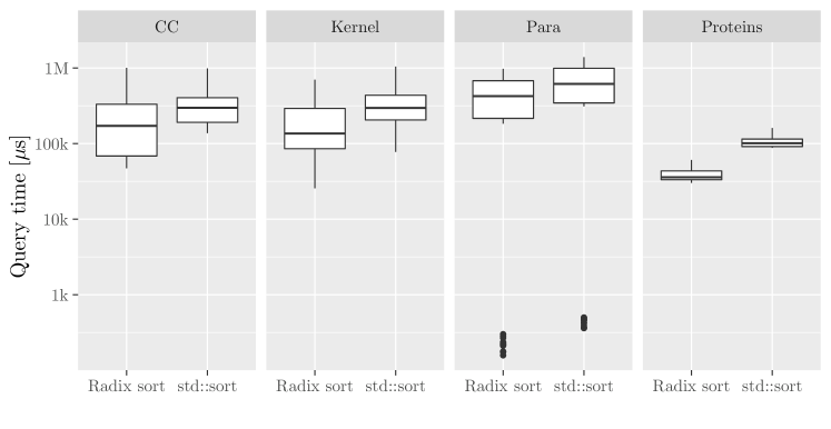
Figure 2: Time to search a 2GiB subset of the Common Crawl web collection (commoncrawl.org). for 20 VLG patterns ($k=2$, $\delta_{i},\Delta_{i}=\langle 100,110\rangle$), composed of very frequent subpatterns drawn from the 200 most common substrings of length 3 in the collection.

Figure 2 shows the results obtained on our test machine (see Section 5 for specifications). Using radix sort instead of std::sort, SA-scan becomes at least two times faster on the Kernel and Proteins datasets, almost twice as fast on CC, and more than 30% faster on Para. A large if algorithmically-somewhat-unexciting leap forward — but further improvements are possible.

3 Filter, filter, sort, scan

Our first serious embellishment to SA-scan aims to avoid sorting the full set of subpattern occurrences by filtering out some of the candidate positions that cannot possibly lead to matches. Specifically, we allocate a bitvector $F$ of $n/b$ bits initially all set to 0. We refer to $b$ as the block size of the filter. Logically, each bit represents a block of $b$ contiguous positions in the input text, with the $i$th bit corresponding to the positions $ib..i(b+1)-1$. In describing the use of the filter we assume two subpatterns $p_{1}$ and $p_{2}$ (with occurrences in $\mbox{\rm{\sf SA}}[s_{1}..e_{1}]$ and $\mbox{\rm{\sf SA}}[s_{2}..e_{2}]$, respectively), but the technique is easy to generalize for $k>2$.

Having allocated $F$, we scan the interval $\mbox{\rm{\sf SA}}[s_{1}..e_{1}]$ containing the occurrences of subpattern $p_{1}$ and for each element $i=SA[j]$ encountered, we set bits $F[(i+\delta)/b..(i+\Delta)/b]$ to $1$ to indicate that an occurrence of $p_{2}$ in any of the corresponding blocks of the input is a potential match. During the scan we also copy elements of the interval to an array $A_{1}$ of size $m_{1}=e_{1}-s_{1}+1$. We then scan the interval $\mbox{\rm{\sf SA}}[s_{2}..e_{2}]$ containing the occurrences of the second subpattern and for each position $i$ encountered we check $F[i/b]$. If $F[i/b]=0$ then $i$ cannot possibly be part of a match and can be discarded. Otherwise ($F[i/b]=1$) we add $i$ to a vector $A_{2}$ of candidates. We then sort $A_{1}$ and $A_{2}$ and intersect them with respect to the gap constraints, the same as in the original SA-scan algorithm. The hope is that $|A_{2}|$ is much less than $e_{2}-s_{2}+1$, and so the time spent sorting prior to intersection will be reduced.

There are two straightforward refinements to this approach. The first is to make the initial scan not necessarily over $\mbox{\rm{\sf SA}}[s_{1}..e_{1}]$, but instead over the smaller of intervals $\mbox{\rm{\sf SA}}[s_{1}..e_{1}]$ and $\mbox{\rm{\sf SA}}[s_{2}..e_{2}]$. The only difference is that if the interval for $p_{2}$ (the second subpattern) happens to be smaller (i.e. $p_{2}$ has less occurrences in T than $p_{1}$) then we set bits $F[(i-\delta)/b..(i-\Delta)/b]$ (rather than $F[(i+\delta)/b..(i+\Delta)/b]$) to 1. Assuming $p_{1}$ is in fact more frequent than $p_{2}$, the second refinement is to perform a second round of filtering using the contents of $A_{2}$. More precisely, having obtained $A_{2}$, we clear $F$ (setting all bits to 0) and scan $A_{2}$ settings bits $F[(i-\delta)/b..(i-\Delta)/b]$ to 1 for each $i\in A_{2}$. We then scan $A_{1}$ and discard any element $i$ for which $F[i/b]$ now equals 0. Obviously it only makes sense to employ this heuristic if the initial filtering reduced the number of candidates, $|A_{2}|$, of the second subpattern significantly below $m_{1}$. In practice we found $m_{2}<m_{1}/2$ led to a consistent speedup.

Of course, these techniques generalize easily to $k>2$ subpatterns. The idea is that the output of the intersection of the first two subpatterns then becomes an input interval to be intersected with the third subpattern, and so on.

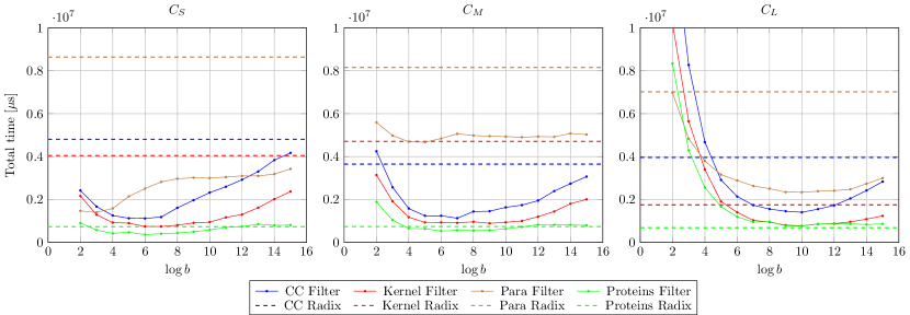
Figure 3: Effect of filter granularity on search time. Ordinate is runtime in microseconds and mantissa is the logarithm (base 2) of the filter block size. Dashed lines show the time required by SA-scan (using radix sort) without any filter. Each plot corresponds to a different set of 20 synthetically generated VLG patterns. All patterns contain 2 of the 200 most frequent subpatterns in each data set. We fixed the gap constraints $C_{i}=\langle\delta_{i},\Delta_{i}\rangle$ between subpatterns to small ($C_{S}=\langle 100,110\rangle$), medium ($C_{M}=\langle 1000,1100\rangle$), or large ($C_{L}=\langle 10000,11000\rangle$). Section 5 gives more details of data sets and pattern sets.

As Figure 3 shows, employing $F$ can reduce runtime immensely, but the improvement varies greatly with $b$. A good choice for $b$ depends on a number of factors. For each occurrence of $p_{1}$, we set $\lceil\frac{\Delta-\delta}{b}\rceil$ bits in $F$. Accesses to $F$ while setting these bits are essentially random (determined by the order of the positions of $p_{1}$, which are the lexicographic order of the corresponding suffixes of T), and so it helps greatly if $b$ is chosen so that $F$, which has size $n/b$ bits, fits in cache. This can be seen in Figure 3, particularly clearly for the CC, Kernel, and Protein data sets, where performance improves sharply with increasing $b$ until $F$ fits in cache (30MiB on our test machine) where it quickly stablizes (at $\log b=3$ for CC and Kernel, and $\log b=2$ for Protein). Runtimes then remain remain relatively fast and stable until $b$ becomes so large that the filter lacks specificity, from which point performance gradually degrades. Para has the same trend, though it is not immediately obvious — because the data set is smaller (409MB) $F$ already fits in L3 cache when $b=2$. Section 5 gives more details of data sets and pattern sets.

For the large-gap pattern set ($C_{L}$), where $\Delta-\delta=1000$ the optimal choice of $b$ for all data sets is much higher — $b=1024$ in all cases ($b=512$ has very similar performance). Here we are seeing the effect of the time needed to set bits in the filter. For example, for Kernel, $F$ already fits in L3 cache when $b=8$, but at that setting $\lceil\frac{\Delta-\delta}{b}\rceil=1000/8=125$ bits must be set in $F$ per occurrence of $p_{1}$. With $b=1024$ or $512$, the number of bits set in $F$ per occurrence of $p_{1}$ is just 1 or 2, the same as it is at the optimal setting for the small-gap ($C_{S}$) and middle-gap ($C_{M}$) pattern sets. This effect can probably be largely alleviated by employing two levels of filters or, alternatively, by implementing a method for setting a word of 1s at a time (effectively reducing the time to set bits from $\lceil\frac{\Delta-\delta}{b}\rceil$ to $\lceil\frac{\Delta-\delta}{b\cdot w}\rceil$, where $w$ is the word size).

4 Direct text checking

The filtering ideas described in the previous section can drastically reduce the amount of time spent per subpattern occurrence, but the overall runtime is still $\Omega({\mit occ}_{1}+{\mit occ}_{2})$, because both subpattern intervals are scanned in full. When the number of occurrences of the less frequent subpattern, say $p_{1}$, are significantly less than those of $p_{2}$, it is possible to get below that bound by scanning over only the occurrences of $p_{1}$, and for each occurrence, $i$, checking directly in the substring of text $\mbox{\rm{\sf T}}[i+\delta..i+\Delta]$ for any occurrences of $p_{2}$, each of which corresponds to a match (or valid candidate match in the case $k>2$). If we use a linear time pattern matching algorithm such as that by Knuth, Morris, and Pratt [13] to search for the occurrences of $p_{2}$, runtime (for two subpatterns) becomes $\Theta({\mit occ}_{1}\cdot(\Delta-\delta))$.

Employed by itself, this kind of text checking can lead to terrible performance when both ${\mit occ}_{1}$ and ${\mit occ}_{2}$ are large. However, when employed in concert with a filter, it can lead to significant performance gains, particularly in later rounds of intersection when $k>2$. Figure 4 illustrates this for $k=2$, along with the performance of the other versions of SA-scan (Filter and Radix) we have decribed in previous sections. In sum, SA-scan has been sped up by more than an order of magnitude on some data sets. In Fig. 5 we see that the text checking heuristic makes an even bigger improvement when the number of subpatterns increases (from $k=2$ to $k=4$) because it is employed more often.

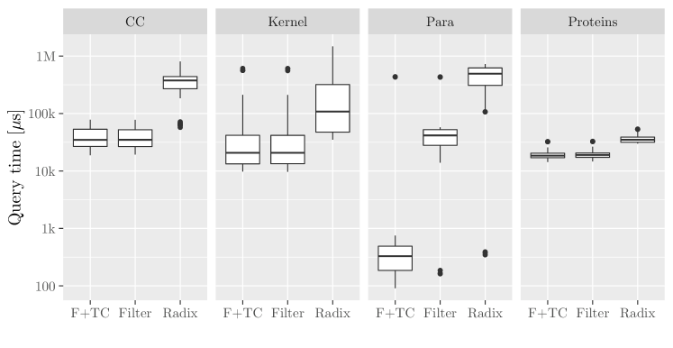
Figure 4: Direct text checking improves search times further ($k=2$).

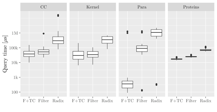
Figure 5: Direct text checking improves search times further ($k=4$).

5 Experimental Evaluation

In this section we compare the practical performance of our version of SA-scan to the wavelet-tree-based method of Bader et al., which is called WT. We use a variety of texts and patterns, which are detailed below (most of these have appeared in experiments described in previous sections). Our methodology in this section closely follows that of [1].

Test Machine and Environment.

We used a 2.10 GHz Intel Xeon E7-4830 v3 CPU equipped with 30 MiB L3 cache and 1.5 TiB of main memory. The machine had no other significant CPU tasks running and only a single thread of execution was used. The OS was Linux (Ubuntu 16.04, 64bit) running kernel 4.10.0-38-generic. Programs were compiled using g++ version 5.4.0.

Texts.

We use five datasets from different application domains:

• CC is a 2 GiB prefix of a recent 145TiB web crawl from commoncrawl.org.

• Kernel is a 2 GiB file consisting of source code of all (332) Linux kernel versions $2.2.X$, $2.4.X.Y$ and $2.6.X.Y$ downloaded from kernel.org. The data set is very repetitive as only minor changes exist between subsequent versions.

• Para is a 410 MiB, which contains 36 sequences of Saccharomyces Paradoxus, is provided by the Saccharomyces Genome Resequencing Project. There are four bases $\{A,C,G,T\}$, but some characters denote an unknown choice among the four bases in which case $N$ is used.

• Proteins is a 1.2 GiB sequence of newline-separated protein sequences (without descriptions, just the bare proteins) obtained from the Swissprot database. Each of the 20 amino acids is coded as one letter.

Patterns.

As in [4], patterns were generated synthetically for each data set. We fixed the gap constraints $C_{i}=\delta_{i},\Delta_{i}$ between subpatterns to small ($C_{S}=\langle 100,110\rangle$), medium ($C_{M}=\langle 1000,1100\rangle$), or large ($C_{L}=\langle 10000,11000\rangle$). VLG patterns were generated by extracting the 200 most common substrings of lengths 3, 5, and 7, which are then used as subpatterns. We then form 20 VLG patterns for each dataset, $k$ (i.e. number of subpatterns), and gap constraint by selecting from the set of 200 subpatterns. We emphasise that the generated patterns, while not specifically designed to be pathological, do represent relatively hard instances for SA-scan because of the high frequency of each subpattern.

Matching Performance for Different Gap Constraint Bands.

Our first experiment aims to elucidate the impact of gap constraint size on query time. We fix the subpattern length $|p_{i}|=m_{i}=3$. Table 1 shows the results from VLG patterns consisting of $k=2^{1},\ldots,2^{5}$ subpatterns. Our method, marked Filter+TC, is always faster than WT, with the exception of the large-gap $C_{L}$ pattern sets, where on some data sets it yields to WT (most likely due to the text-checking heuristic being less effective on $C_{L}$).

Method CC Kernel Para Proteins $C_{S}$ $C_{M}$ $C_{L}$ $C_{S}$ $C_{M}$ $C_{L}$ $C_{S}$ $C_{M}$ $C_{L}$ $C_{S}$ $C_{M}$ $C_{L}$ k = 2 Filter+TC 1391 1783 3329 744 1303 2243 2243 4170 2184 388 485 976 WT_ALL 17354 19736 21757 7393 10205 15891 12372 14683 3654 8549 10547 14470 k = 4 Filter+TC 1099 1739 3186 664 1158 1654 1214 8134 9036 370 580 1609 WT_ALL 7452 7499 8770 2201 4810 2756 6554 9039 5230 8486 9319 12621 k = 8 Filter+TC 2185 1219 3057 328 733 3563 5 27 10300 354 581 2231 WT_ALL 7919 6511 6054 1885 2260 1468 237 345 2518 11940 12867 13450 k = 16 Filter+TC 674 930 3267 312 667 984 5 15 631 350 534 2361 WT_ALL 7483 5580 7827 948 1497 1540 279 260 249 20950 21811 23501 k = 32 Filter+TC 510 649 2193 369 327 634 5 14 541 342 528 2326 WT_ALL 10358 13142 11564 1973 1696 1617 496 517 498 46232 47935 48784

Table 1: Total query time in milliseconds on all data sets for fixed $m_{i}=3$ and gap constraints $C_{S}=\langle 100,110\rangle$, $C_{M}=\langle 1000,1100\rangle$, and $C_{L}=\langle 10000,11000\rangle$.

Matching Performance for Different Subpattern Lengths.

In our second experiment, we examine the impact of subpattern lengths on query time, fixing the gap constraint to $C_{S}=100,110$. Table 2 shows the results. Larger subpattern lengths tend to result in smaller SA ranges. Consequently, SA-scan outperforms WT by an even wider margin.

Method CC Kernel Para Proteins 3 5 7 3 5 7 3 5 7 3 5 7 k = 2 Filter+TC 1391 478 321 744 304 84 2243 629 75 388 33 24 WT_ALL 17354 4535 2995 7393 1725 94 12372 9911 2435 8549 427 172 k = 4 Filter+TC 1099 327 179 664 132 64 1214 742 67 370 32 21 WT_ALL 7452 2030 512 2201 145 31 6554 10908 2414 8486 96 68 k = 8 Filter+TC 2185 227 100 328 133 116 5 628 66 354 28 25 WT_ALL 7919 1395 466 1885 154 47 237 16475 3563 11940 48 33 k = 16 Filter+TC 674 228 140 312 90 50 5 675 65 350 28 33 WT_ALL 7483 925 365 948 129 80 279 29231 6222 20950 83 61 k = 32 Filter+TC 510 192 109 369 117 85 5 563 65 342 32 28 WT_ALL 10358 1464 548 1973 274 167 496 64780 13435 46232 181 131

Table 2: Total query time in milliseconds for fixed gap constraint $C_{S}=\langle 100,110\rangle$ for different subpattern lengths $m_{i}\in\{3,5,7\}$ and different data sets.

Overall Runtime Performance.

In a final experiment we explored the whole parameter space (i.e. $k\in\{2^{1},\ldots,2^{5}\}$, $m_{i}\in\{3,5,7\}$, $C\in\{C_{S},C_{M},C_{L}\}$). The results are summarized in Figure 6. Overall out SA-scan-based method is faster on average than the wavelet-tree-based one, usually by a wide margin.

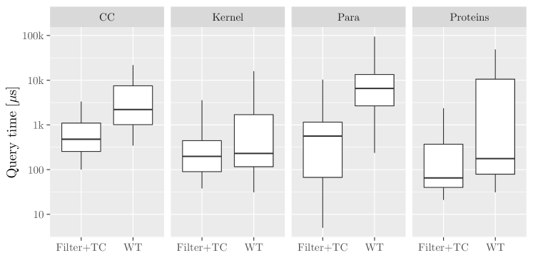
Figure 6: Overall runtime performance of both methods, accumulating the performance for all $m_{i}\in\{3,5,7\}$ and $C_{S}$, $C_{M}$, and $C_{L}$.

6 Concluding Remarks

We have described a number of simple but highly effective improvements to the SA-scan VLG matching algorithm that, according to our experiments, elevate it to be the state-of-the-art approach for the indexed version of problem. We believe better indexing methods for VLG matching can be found, but that our version of SA-scan, which makes judicious use of filters, text checking, and subpattern processing order, represents a strong baseline against which the performance of more exotic methods should be measured.

Numerous avenues for continued work on VLG matching exist, perhaps the most interesting of which is to reduce index size. Currently, SA-scan uses $n\log n+n\log\sigma$ bits of space for a text of length $n$ on alphabet $\sigma$ for the suffix array and text, respectively (the WT approach of Bader et al., uses slightly more). Because our methods consist (mostly) of simple scans of SA ranges or scans of the underlying text, they are easily translated to make use of recent results on Burrows-Wheeler-based compressed indexes [10] that allow fast access to elements of the suffix array from a compressed representation of it. Via this observation we derive the first compressed indexes for VLG matching. These indexes use $O(r\log n)$ bits of space, where $r$ is the number of runs in the Burrows-Wheeler transform, a quantity that decreases with text compressibility. On our 2 GiB Kernel data set, for example, the compressed index takes around 20 MiB in practice, and can still support VLG matching in times competitive with the indexes of Bader et al. We plan to explore this in more depth in future work.

Acknowledgements.

Our thanks go to Tania Starikovskaya for suggesting the problem of indexing for regular-expression matching to us. We also thank Matthias Petri and Simon Gog for prompt answers to questions about their article and code and the anonymous reviewers for helpful comments. This work was funded by the Academy of Finland via grant 319454 and by EU’s Horizon 2020 research and innovation programme under Marie Skłodowska-Curie grant agreement No 690941 (BIRDS).

References

- [1] Bader, J., Gog, S., Petri, M.: Practical variable length gap pattern matching. In: Goldberg, A.V., Kulikov, A.S. (eds.) Proc. SEA. pp. 1–16. LNCS 9685 (2016)
- [2] Bille, P., Farach-Colton, M.: Fast and compact regular expression matching. Theor. Comput. Sci. 409(3), 486–496 (2008)
- [3] Bille, P., Gortz, I.L.: Substring range reporting. Algorithmica 69(2), 384–396 (2014)
- [4] Bille, P., Gortz, I.L., Vildhoj, H.W., Wind, D.K.: String matching with variable length gaps. Theor. Comput. Sci. 443, 25–34 (2012)
- [5] Bille, P., Thorup, M.: Regular expression matching with multi-strings and intervals. In: Proc. SODA. pp. 1297–1308. ACM-SIAM (2010)
- [6] Cox, R.: Regular expression matching with a trigram index or how Google code search worked (2012), https://swtch.com/~rsc/regexp/regexp4.html
- [7] Crawford, T., Iliopoulos, C.S., Raman, R.: String matching techniques for musical similarity and melodic recognition. Computing in Musicology 11, 73–100 (1998)
- [8] Crochemore, M., Iliopoulos, C.S., Makris, C., Rytter, W., Tsakalidis, A.K., Tsichlas, T.: Approximate string matching with gaps. N. J. Comput. 9(1), 54–65 (2002)
- [9] Fredriksson, K., Grabowski, S.: Efficient algorithms for pattern matching with general gaps, character classes, and transposition invariance. Inf. Retr. 11(4), 335–357 (2008)
- [10] Gagie, T., Navarro, G., Prezza, N.: Optimal-time text indexing in BWT-runs bounded space. In: Proc. SODA. pp. 1459–1477. ACM-SIAM (2018)
- [11] Grossi, R., Gupta, A., Vitter, J.: High-order entropy-compressed text indexes. In: Proc. SODA. pp. 841–850. ACM-SIAM (2003)
- [12] Haapasalo, T., Silvasti, P., Sippu, S., Soisalon-Soininen, E.: Online dictionary matching with variable-length gaps. In: Proc. SEA. pp. 76–87. LNCS 6630 (2011)
- [13] Knuth, D., Morris, J.H., Pratt, V.: Fast pattern matching in strings. SIAM Journal on Computing 6(2), 323–350 (1977)
- [14] Lewenstein, M.: Indexing with gaps. In: Proc. SPIRE. pp. 135–143. LNCS 7024, Springer (2011)
- [15] Lopez, A.: Hierarchical phrase-based translation with suffix arrays. In: Proc. EMNLP-CoNLL 2007. pp. 976–985. ACL (2007)
- [16] Manber, U., Myers, G.: Suffix arrays: a new method for on-line string searches. SIAM J. Computing 22(5), 935–948 (1993)
- [17] Metzler, D., Croft, W.B.: A markov random field model for term dependencies. In: Proc. SIGIR. pp. 472–479. ACM (2005)
- [18] Morgante, M., Policriti, A., Vitacolonna, N., Zuccolo, A.: Structured motifs search. Journal of Computational Biology 12(8), 1065–1082 (2005)
- [19] Navarro, G.: Wavelet trees for all. Journal of Discrete Algorithms 25, 2–20 (2014)
- [20] Pissis, S.P.: MoTeX-II: structured MoTif eXtraction from large-scale datasets. BMC Bioinformatics 15(235), 1–12 (2014)
- [21] Saikkonen, R., Sippu, S., Soisalon-Soininen, E.: Experimental analysis of an online dictionary matching algorithm for regular expressions with gaps. In: Proc. SEA. pp. 327–338. LNCS 9125, Springer (2015)
- [22] Turpin, A., Tsegay, Y., Hawking, D., Williams, H.E.: Fast generation of result snippets in web search. In: Proc. SIGIR 2007. pp. 127–134. ACM (2007)