On Biased Compression for Distributed Learning

Abstract

In the last few years, various communication compression techniques have emerged as an indispensable tool helping to alleviate the communication bottleneck in distributed learning. However, despite the fact biased compressors often show superior performance in practice when compared to the much more studied and understood unbiased compressors, very little is known about them. In this work we study three classes of biased compression operators, two of which are new, and their performance when applied to (stochastic) gradient descent and distributed (stochastic) gradient descent. We show for the first time that biased compressors can lead to linear convergence rates both in the single node and distributed settings. We prove that distributed compressed SGD method, employed with error feedback mechanism, enjoys the ergodic rate ${\cal O}\left(\delta L\exp[-\frac{\mu K}{\delta L}]+\frac{(C+\delta D)}{K\mu}\right)$, where $\delta\geq 1$ is a compression parameter which grows when more compression is applied, $L$ and $\mu$ are the smoothness and strong convexity constants, $C$ captures stochastic gradient noise ($C=0$ if full gradients are computed on each node) and $D$ captures the variance of the gradients at the optimum ($D=0$ for over-parameterized models). Further, via a theoretical study of several synthetic and empirical distributions of communicated gradients, we shed light on why and by how much biased compressors outperform their unbiased variants. Finally, we propose several new biased compressors with promising theoretical guarantees and practical performance.

Keywords: Compression operators, biased compressors, distributed learning, linear convergence, error feedback

1 Introduction

In order to achieve state-of-the-art performance, modern machine learning models need to be trained using large corpora of training data, and often feature an even larger number of trainable parameters (Vaswani et al., 2019; Brown et al., 2020). The data is typically collected in a distributed manner and stored across a network of edge devices, as is the case in federated learning (Konečný et al., 2016; McMahan et al., 2017; Li et al., 2019; Kairouz and et al, 2019), or collected centrally in a data warehouse composed of a large collection of commodity clusters. In either scenario, communication among the workers is typically the bottleneck.

Motivated by the need for more efficient training methods in traditional distributed and emerging federated environments, we consider optimization problems of the form

$$\min\limits_{x\in\mathbb{R}^{d}}\left\{f(x)\coloneqq\frac{1}{n}\sum\limits_{i=1}^{n}f_{i}(x)\right\}\,,$$ (1)

where $x\in\mathbb{R}^{d}$ collects the parameters of a statistical model to be trained, $n$ is the number of workers/devices, and $f_{i}(x)$ is the loss incurred by model $x$ on data stored on worker $i$. The loss function $f_{i}:\mathbb{R}^{d}\to\mathbb{R}$ often has the form

$$f_{i}(x)\coloneqq{\rm E}_{\xi\sim{\cal P}_{i}}\left[f_{\xi}(x)\right],$$

with ${\cal P}_{i}$ being the distribution of training data owned by worker $i$. In federated learning applications, these local distributions can be very different and we do not impose any similarity assumption for them.

1.1 Distributed optimization

A fundamental baseline for solving problem (1) is (distributed) gradient descent (GD), performing updates of the form

$$x^{k+1}=x^{k}-\frac{\eta^{k}}{n}\sum\limits_{i=1}^{n}\nabla f_{i}(x^{k}),$$

where $\eta^{k}>0$ is a stepsize. Due to the communication issues inherent to distributed systems, several enhancements to this baseline have been proposed that can better deal with the communication cost challenges of distributed environments, including acceleration (Nesterov, 2013; Beck and Teboulle, 2009; Allen-Zhu, 2017), reducing the number of iterations via momentum, local methods (McMahan et al., 2017; Khaled et al., 2020a; Karimireddy et al., 2019a), reducing the number of communication rounds via performing multiple local updates before each communication round, and communication compression (Seide et al., 2014; Alistarh et al., 2017; Zhang et al., 2017; Lim et al., 2018; Alistarh et al., 2018; Lin et al., 2018; Safaryan and Richtárik, 2021), reducing the size of communicated messages via compression operators.

1.2 Contributions

In this paper we contribute to a better understanding of the latter approach to alleviating the communication bottleneck: communication compression. In particular, we study the theoretical properties of gradient-type methods which employ biased gradient compression operators, such as Top-$k$ sparsification (Alistarh et al., 2018), or deterministic rounding (Sapio et al., 2019). Surprisingly, current theoretical understanding of such methods is very limited. For instance, there is no general theory of such methods even in the $n=1$ case, only a handful of biased compression techniques have been proposed in the literature, we do not have any theoretical understanding of why biased compression operators could outperform their unbiased counterparts and when. More importantly, there is no good convergence theory for any gradient-type method with a biased compression in the crucial $n>1$ setting.

In this work we address all of the above problems. In particular, our main contributions are:

• We define and study three parametric classes of biased compression operators (see Section 2), which we denote $\mathbb{B}^{1}(\alpha,\beta)$, $\mathbb{B}^{2}(\gamma,\beta)$ and $\mathbb{B}^{3}(\delta)$, the first two of which are new. We prove that, despite they are alternative parameterization of the same collection of operators, the last two are more favorable than the first one, thus highlighting the importance of parametrization and providing further reductions. We show how is the commonly used class of unbiased compression operators, which we denote $\mathbb{U}(\zeta)$, relates to these biased classes. We also study scaling and compositions of such compressors.

• We then proceed to give a long list of new and known biased (and some unbiased) compression operators which belong to the above classes in Section 2.2. A summary of all compressors considered can be found in Table 3.

• In Section 3 we analyze compressed GD in the $n=1$ case for compressors belonging to all three classes under smoothness and strong convexity assumption. Our theorems generalize existing results which hold for unbiased operators in a tight manner, and also recover the rate of GD in this regime. Our linear convergence results are summarized in Table 1.

  Compressor	${\cal C}\in\mathbb{B}^{1}(\alpha,\beta)$	${\cal C}\in\mathbb{B}^{2}(\gamma,\beta)$	${\cal C}\in\mathbb{B}^{3}(\delta)$
  Theorem	Theorem 17	Theorem 18	Theorem 19
  Complexity	$\displaystyle{\cal O}\left(\frac{\beta^{2}}{\alpha}\frac{L}{\mu}\log\frac{1}{\epsilon}\right)$	$\displaystyle{\cal O}\left(\frac{\beta}{\gamma}\frac{L}{\mu}\log\frac{1}{\epsilon}\right)$	$\displaystyle{\cal O}\left(\delta\frac{L}{\mu}\log\frac{1}{\epsilon}\right)$

  Table 1: Complexity results for GD with biased compression. The identity compressor ${\cal C}(x)\equiv x$ belongs to all classes with $\alpha=\beta=\gamma=\delta=1$; all three results recover standard rate of GD.

• We ask the question: do biased compressors outperform their unbiased counterparts in theory, and by how much? We answer this question by studying the performance of compressors under various synthetic and empirical statistical assumptions on the distribution of the entries of gradient vectors which need to be compressed. Particularly, we quantify the gains of the Top-$k$ sparsifier when compared against the unbiased Rand-$k$ sparsifier in Section 4.

• Finally, we study the important $n>1$ setting in Section 5 and argue by giving a counterexample that a naive application of biased compression to distributed GD might diverge. We then show that distributed SGD method equipped with an error-feedback mechanism (Stich and Karimireddy, 2019) provably handles biased compressors. In our main result (Theorem 21; also see Table 2) we consider three learning schedules and iterate averaging schemes to provide three distinct convergence rates. Our analysis provides the first convergence guarantee for distributed gradient-type method which provably converges for biased compressors, and we thus solve a major open problem in the literature.

  Stepsizes	Weights	Rate
  ${\cal O}(\frac{1}{k})$	${\cal O}(k)$	$\displaystyle{\cal O}\left(\frac{A_{1}}{K^{2}}+\frac{A_{2}}{K}\right)$
  ${\cal O}(1)$	${\cal O}(e^{-k})$	$\displaystyle\tilde{\cal O}\left(A_{3}\exp\left[-\frac{K}{A_{4}}\right]+\frac{A_{2}}{K}\right)$
  ${\cal O}(1)$	$1$	$\displaystyle{\cal O}\left(\frac{A_{3}}{K}+\frac{A_{5}}{\sqrt{K}}\right)$

  Table 2: Ergodic convergence of distributed SGD with biased compression and error-feedback (Algorithm 1) for $L$-smooth and $\mu$-strongly convex functions ($K$ communications). Details are given in Theorem 21.

1.3 Related work

There has been extensive work related to communication compression, mostly focusing on unbiased compressions (Alistarh et al., 2017) as these are much easier to analyze. In particular, it was shown (Gorbunov et al., 2020a) that both the classical method with unbiased compression (Alistarh et al., 2017) and more advanced modifications (Mishchenko et al., 2019; Horváth et al., 2019b) can be considered as special versions of SGD. Subsequently, the results of (Gorbunov et al., 2020a) for strongly convex problems were transferred to general convex (Khaled et al., 2020b) and non-convex  (Li and Richtárik, 2020) target functions. In the meantime, works concerning biased compressions show stronger empirical results but with limited or no analysis (Vogels et al., 2019; Lin et al., 2017a; Sun et al., 2019). There have been several attempts trying to address this issue, e.g., Wu et al. (2018) provided analysis for quadratics in distributed setting, Zhao et al. (2019) gave analysis for momentum SGD with a specific biased compression, but under unreasonable assumptions, i.e., bounded gradient norm and memory. The first result that obtained linear rate of convergence for biased compression was done by Karimireddy et al. (2019b), but only for one node and under bounded gradient norm assumption, which was later overcome by Stich and Karimireddy (2019).

After the initial online appearance of our work, there has been several enhancements in the literature. In particular, Ajalloeian and Stich (2021) developed theory for non-convex objectives in the single node setup, Gorbunov et al. (2020b) designed a novel error compansated SGD algorithm converging linearly in a more relaxed setting with the help of additional unbiased compressor, Horváth and Richtárik (2021) proposed a simple trick to convert any biased compressor to corresponding induced (unbiased) compressor leading to improved theoretical guarantees. Recently, a new variant of error feedback mechanism was introduced in (Richtárik et al., 2021; Fatkhullin et al., 2021) showing an improved rates for distributed non-convex problems.

1.4 Basic notation and definitions

We use $\langle x,y\rangle\coloneqq\sum_{i=1}^{d}x_{i}y_{i}$ to denote standard inner product of $x,y\in\mathbb{R}^{d}$, where $x_{i}$ corresponds to the $i$-th component of $x$ in the standard basis in $\mathbb{R}^{d}$. This induces the $\ell_{2}$-norm in $\mathbb{R}^{d}$ in the following way $\left\|x\right\|_{2}\coloneqq\sqrt{\langle x,x\rangle}$. We denote $\ell_{p}$-norms as $\|x\|_{p}\coloneqq(\sum_{i=1}^{d}|x_{i}|^{p})^{\nicefrac{{1}}{{p}}}$ for $p\in(1,\infty)$. By ${{\rm E}}\left[\cdot\right]$ we denote mathematical expectation. For a given differentiable function $f:\mathbb{R}^{d}\to\mathbb{R}$, we say that it is $L$-smooth if

$$f(y)\leq f(x)+\langle\nabla f(x),y-x\rangle+\frac{L}{2}\left\|y-x\right\|_{2}^{2},\qquad\forall x,y\in\mathbb{R}^{d}.$$

We say that it is $\mu$-strongly convex if

$$f(y)\geq f(x)+\langle\nabla f(x),y-x\rangle+\frac{\mu}{2}\left\|y-x\right\|_{2}^{2},\qquad\forall x,y\in\mathbb{R}^{d}.$$

2 Biased Compressors

By compression operator we mean a (possibly random) mapping ${\cal C}\colon\mathbb{R}^{d}\to\mathbb{R}^{d}$ with some constraints. Typically, literature considers unbiased compression operators ${\cal C}$ with a bounded second moment, i.e.

Definition 1

Let $\zeta\geq 1$. We say that ${\cal C}\in\mathbb{U}(\zeta)$ if ${\cal C}$ is unbiased (i.e., ${{\rm E}}\left[{\cal C}(x)\right]=x$ for all $x$) and if the second moment is bounded as

$${{\rm E}}\left[\left\|{\cal C}(x)\right\|_{2}^{2}\right]\leq\zeta\left\|x\right\|_{2}^{2},\qquad\forall x\in\mathbb{R}^{d}\,.$$ (2)

2.1 Three classes of biased compressors

We instead focus on understanding biased compression operators, or “compressors” in short. We now introduce three classes of biased compressors, the first two are new, which can be seen as natural extensions of unbiased compressors.

Definition 2

We say that ${\cal C}\in\mathbb{B}^{1}(\alpha,\beta)$ for some $\alpha,\beta>0$ if

$$\alpha\left\|x\right\|_{2}^{2}\leq{{\rm E}}\left[\left\|{\cal C}(x)\right\|_{2}^{2}\right]\leq\beta\langle{{\rm E}}\left[{\cal C}(x)\right],x\rangle,\qquad\forall x\in\mathbb{R}^{d}\;.$$ (3)

As we shall show next, the second inequality in (3) implies ${{\rm E}}\left[\left\|{\cal C}(x)\right\|_{2}^{2}\right]\leq\beta^{2}\left\|x\right\|_{2}^{2}$.

Lemma 3

For any $x\in\mathbb{R}^{d}$, if ${{\rm E}}\left[\left\|{\cal C}(x)\right\|_{2}^{2}\right]\leq\beta\langle{{\rm E}}\left[{\cal C}(x)\right],x\rangle$, then

$${{\rm E}}\left[\left\|{\cal C}(x)\right\|_{2}^{2}\right]\leq\beta^{2}\left\|x\right\|_{2}^{2}.$$ (4)

Proof  Fix any $x\in\mathbb{R}^{d}$. Applying Jensen’s inequality, the second inequality in (3) and Cauchy-Schwarz, we get

$$\left\|{{\rm E}}\left[{\cal C}(x)\right]\right\|_{2}^{2}\leq{{\rm E}}\left[\left\|{\cal C}(x)\right\|_{2}^{2}\right]\overset{\eqref{eq:alpha-beta}}{\leq}\beta\langle{{\rm E}}\left[{\cal C}(x)\right],x\rangle\leq\beta\left\|{{\rm E}}\left[{\cal C}(x)\right]\right\|_{2}\left\|x\right\|_{2}.$$ (5)

If ${{\rm E}}\left[{\cal C}(x)\right]\neq 0$, this implies $\left\|{{\rm E}}\left[{\cal C}(x)\right]\right\|_{2}\leq\beta\left\|x\right\|_{2}$. Plugging this back into (5), we get (4). If ${{\rm E}}\left[{\cal C}(x)\right]=0$, then from (3) we see that ${{\rm E}}\left[\left\|{\cal C}(x)\right\|_{2}^{2}\right]=0$, and (4) holds trivially.  

In the second class, we require the inner product between uncompressed $x$ and compressed ${\cal C}(x)$ vectors to dominate the squared norms of both vectors in expectation.

Definition 4

We say that ${\cal C}\in\mathbb{B}^{2}(\gamma,\beta)$ for some $\gamma,\beta>0$ if

$$\max\left\{\gamma\left\|x\right\|_{2}^{2},\tfrac{1}{\beta}{{\rm E}}\left[\left\|{\cal C}(x)\right\|_{2}^{2}\right]\right\}\leq\langle{{\rm E}}\left[{\cal C}(x)\right],x\rangle\qquad\forall x\in\mathbb{R}^{d}\,.$$ (6)

Finally, in the third class, we require the compression error $\left\|{\cal C}(x)-x\right\|_{2}^{2}$ to be strictly smaller than the squared norm $\left\|x\right\|_{2}^{2}$ of the input vector $x$ in expectation.

Definition 5

We say ${\cal C}\in\mathbb{B}^{3}(\delta)$ for some $\delta>0$ if

$${{\rm E}}\left[\left\|{\cal C}(x)-x\right\|_{2}^{2}\right]\leq\left(1-\frac{1}{\delta}\right)\left\|x\right\|_{2}^{2},\qquad\forall x\in\mathbb{R}^{d}\;.$$ (7)

This last definition was also considered by Stich et al. (2018); Cordonnier (2018). All three definitions require the compressed vector ${\cal C}(x)$ to be in the neighborhood of the uncompressed vector $x$ so that initial information is preserved with some accuracy. We now establish several basic properties and connections between the classes. We first show that the three classes of biased compressors defined above are equivalent in the following sense: a compressor from any of those three classes can be shown to belong to all three classes with different parameters and after possible scaling.

Theorem 6 (Equivalence between biased compressors)

Let $\lambda>0$ be a free scaling parameter.

1. If ${\cal C}\in\mathbb{B}^{1}(\alpha,\beta)$, then

   • $\beta^{2}\geq\alpha$ and $\lambda{\cal C}\in\mathbb{B}^{1}(\lambda^{2}\alpha,\lambda\beta)$, and

   • ${\cal C}\in\mathbb{B}^{2}(\alpha/\beta,\beta)$ and $\frac{1}{\beta}{\cal C}\in\mathbb{B}^{3}(\beta^{2}/\alpha)$.

2. If ${\cal C}\in\mathbb{B}^{2}(\gamma,\beta)$, then

   • $\beta\geq\gamma$ and $\lambda{\cal C}\in\mathbb{B}^{2}(\lambda\gamma,\lambda\beta)$, and

   • ${\cal C}\in\mathbb{B}^{1}(\gamma^{2},\beta)$ and $\frac{1}{\beta}{\cal C}\in\mathbb{B}^{3}(\beta/\gamma)$.

3. If ${\cal C}\in\mathbb{B}^{3}(\delta)$, then

   • $\delta\geq 1$, and

   • ${\cal C}\in\mathbb{B}^{2}\left(\frac{1}{2\delta},2\right)\subseteq\mathbb{B}^{1}\left(\frac{1}{4\delta^{2}},2\right)$.

Proof  Let us prove this implications for each class separately.

1. Case ${\cal C}\in\mathbb{B}^{1}(\alpha,\beta)$:

   • Let us choose any $x\neq 0$ and observe that (3) implies that ${{\rm E}}\left[{\cal C}(x)\right]\neq 0$. Further, from (3) we get the bounds

     $$\frac{{{\rm E}}\left[\left\|{\cal C}(x)\right\|_{2}^{2}\right]}{\langle{{\rm E}}\left[{\cal C}(x)\right],x\rangle}\leq\beta,\qquad\alpha\leq\frac{{{\rm E}}\left[\left\|{\cal C}(x)\right\|_{2}^{2}\right]}{\left\|x\right\|_{2}^{2}}.$$

     Finally,

     $$\beta^{2}\geq\left(\frac{{{\rm E}}\left[\left\|{\cal C}(x)\right\|_{2}^{2}\right]}{\langle{{\rm E}}\left[{\cal C}(x)\right],x\rangle}\right)^{2}\geq\frac{{{\rm E}}\left[\left\|{\cal C}(x)\right\|_{2}^{2}\right]{{\rm E}}\left[\left\|{\cal C}(x)\right\|_{2}^{2}\right]}{\left\|{{\rm E}}\left[{\cal C}(x)\right]\right\|_{2}^{2}\left\|x\right\|_{2}^{2}}\geq\alpha\frac{{{\rm E}}\left[\left\|{\cal C}(x)\right\|_{2}^{2}\right]}{\left\|{{\rm E}}\left[{\cal C}(x)\right]\right\|_{2}^{2}}\geq\alpha,$$

     where the second inequality is due to Cauchy-Schwarz, and the last inequality follows by applying Jensen inequality.

     The scaling property $\lambda{\cal C}\in\mathbb{B}^{1}(\alpha\lambda^{2},\beta\lambda)$ follows directly from (3).

   • The inclusion ${\cal C}\in\mathbb{B}^{2}(\alpha/\beta,\beta)$ follows directly from inequalities (3) and (6). In view of (i), $\lambda{\cal C}\in\mathbb{B}^{1}(\lambda^{2}\alpha,\lambda\beta)$. If we choose $\lambda\leq\frac{2}{\beta}$, then

     $${{\rm E}}\left[\left\|\lambda{\cal C}(x)-x\right\|_{2}^{2}\right] = {{\rm E}}\left[\left\|\lambda{\cal C}(x)\right\|_{2}^{2}\right]-2\langle{{\rm E}}\left[\lambda{\cal C}(x)\right],x\rangle+\left\|x\right\|_{2}^{2}$$

     $$\overset{\eqref{eq:alpha-beta}}{\leq} (\beta\lambda-2)\langle{{\rm E}}\left[\lambda{\cal C}(x)\right],x\rangle+\left\|x\right\|_{2}^{2}$$

     $$\overset{\eqref{eq:alpha-beta}}{\leq} (\beta\lambda-2)\frac{\alpha\lambda^{2}}{\beta\lambda}\left\|x\right\|_{2}^{2}+\left\|x\right\|_{2}^{2}$$

     $$\overset{\eqref{eq:alpha-beta}}{\leq} \left(\alpha\lambda^{2}-2\frac{\alpha}{\beta}\lambda+1\right)\left\|x\right\|_{2}^{2}.$$

     Minimizing the above expression in $\lambda$, we get $\lambda=\frac{1}{\beta}$, and the result follows.

2. Case ${\cal C}\in\mathbb{B}^{2}(\gamma,\beta)$.

   • Using (6) we get

     $$\gamma\leq\frac{\left<{{\rm E}}\left[{\cal C}(x)\right],x\right>}{\left\|x\right\|_{2}^{2}}\leq\frac{{{\rm E}}\left[\left\|{\cal C}(x)\right\|_{2}^{2}\right]}{\sqrt{{{\rm E}}\left[\left\|{\cal C}(x)\right\|_{2}^{2}\right]\left\|x\right\|_{2}^{2}}}\leq\beta\frac{\left<{{\rm E}}\left[{\cal C}(x)\right],x\right>}{\sqrt{{{\rm E}}\left[\left\|{\cal C}(x)\right\|_{2}^{2}\right]\left\|x\right\|_{2}^{2}}}\leq\beta,$$

     where the first and third inequalities follow from (6) and the third and the last from Cauchy-Schwarz inequality with Jensen inequality.

     The scaling property $\lambda{\cal C}\in\mathbb{B}^{2}(\lambda\gamma,\lambda\beta)$ follows directly from (6).

   • If ${\cal C}\in\mathbb{B}^{2}(\gamma,\beta)$, then ${{\rm E}}\left[\left\|{\cal C}(x)\right\|_{2}^{2}\right]\leq\beta\langle{{\rm E}}\left[{\cal C}(x)\right],x\rangle$ and

     $$\gamma^{2}\left\|x\right\|_{2}^{4}\overset{\eqref{eq:alpha-betaII}}{\leq}\langle{{\rm E}}\left[{\cal C}(x)\right],x\rangle^{2}\leq\left\|{{\rm E}}\left[{\cal C}(x)\right]\right\|_{2}^{2}\left\|x\right\|_{2}^{2}\leq{{\rm E}}\left[\left\|{\cal C}(x)\right\|_{2}^{2}\right]\left\|x\right\|_{2}^{2},$$

     where the second inequality is Cauchy-Schwarz, and the third is Jensen. Therefore, ${\cal C}\in\mathbb{B}^{1}(\gamma^{2},\beta)$.

     Further, for any $\lambda>0$, we get

     $${{\rm E}}\left[\left\|\lambda{\cal C}(x)-x\right\|_{2}^{2}\right] = {{\rm E}}\left[\left\|\lambda{\cal C}(x)\right\|_{2}^{2}\right]-2\langle{{\rm E}}\left[\lambda{\cal C}(x)\right],x\rangle+\left\|x\right\|_{2}^{2}$$

     $$= \lambda^{2}{{\rm E}}\left[\left\|{\cal C}(x)\right\|_{2}^{2}\right]-2\lambda\langle{{\rm E}}\left[{\cal C}(x)\right],x\rangle+\left\|x\right\|_{2}^{2}$$

     $$\overset{\eqref{eq:alpha-betaII}}{\leq} (\lambda\beta-2)\lambda\langle{{\rm E}}\left[{\cal C}(x)\right],x\rangle+\left\|x\right\|_{2}^{2}.$$

     If we choose $\lambda=\frac{1}{\beta}$, then we can continue as follows:

     $${{\rm E}}\left[\left\|\lambda{\cal C}(x)-x\right\|_{2}^{2}\right] \leq -\frac{1}{\beta}\langle{{\rm E}}\left[{\cal C}(x)\right],x\rangle+\left\|x\right\|_{2}^{2}$$

     $$\overset{\eqref{eq:alpha-betaII}}{\leq} \left(1-\frac{\gamma}{\beta}\right)\left\|x\right\|_{2}^{2},$$

     whence $\frac{1}{\beta}{\cal C}\in\mathbb{B}^{3}(\beta/\gamma)$.

3. Case ${\cal C}\in\mathbb{B}^{3}(\delta)$.

   • Pick $x\neq 0$. Since $0\leq{{\rm E}}\left[\left\|{\cal C}(x)-x\right\|_{2}^{2}\right]\leq\left(1-\frac{1}{\delta}\right)\left\|x\right\|_{2}^{2}$ and we assume $\delta>0$, we must necessarily have $\delta\geq 1$.

   • If ${\cal C}\in\mathbb{B}^{3}(\delta)$ then

     $${{\rm E}}\left[\left\|{\cal C}(x)\right\|_{2}^{2}\right]-2\left<{{\rm E}}\left[{\cal C}(x)\right],x\right>+\frac{1}{\delta}\left\|x\right\|_{2}^{2}\leq 0,$$

     which implies that

     $$\frac{1}{2\delta}\left\|x\right\|_{2}^{2}\leq\left<{{\rm E}}\left[{\cal C}(x)\right],x\right>\qquad\text{and}\qquad{{\rm E}}\left[\left\|{\cal C}(x)\right\|_{2}^{2}\right]\leq 2\left<{{\rm E}}\left[{\cal C}(x)\right],x\right>.$$

     Therefore, ${\cal C}\in\mathbb{B}^{2}\left(\frac{1}{2\delta},2\right)\subseteq\mathbb{B}^{1}\left(\frac{1}{4\delta^{2}},2\right)$.

 

Next, we show that, with a proper scaling, any unbiased compressor also belongs to all the three classes of biased compressors.

Theorem 7 (From unbiased to biased with scaling)

If ${\cal C}\in\mathbb{U}(\zeta)$, then for the scaled operator $\lambda{\cal C}$ we have

• $\lambda{\cal C}\in\mathbb{B}^{1}(\lambda^{2},\lambda\zeta)$ for $\lambda>0$,

• $\lambda{\cal C}\in\mathbb{B}^{2}(\lambda,\lambda\zeta)$ for $\lambda>0$,

• $\lambda{\cal C}\in\mathbb{B}^{3}\left(\frac{1}{\lambda(2-\zeta\lambda)}\right)$ for $\zeta\lambda<2$.

Proof  Let ${\cal C}\in\mathbb{U}(\zeta)$.

• Given any $\lambda>0$, consider the scaled operator $\lambda{\cal C}$. We have

  $$\lambda^{2}\left\|x\right\|_{2}^{2}=\left\|{{\rm E}}\left[\lambda{\cal C}(x)\right]\right\|_{2}^{2}\leq{{\rm E}}\left[\left\|\lambda{\cal C}(x)\right\|_{2}^{2}\right]\leq\lambda^{2}\zeta\left\|x\right\|_{2}^{2}=\lambda\zeta\langle{{\rm E}}\left[\lambda{\cal C}(x)\right],x\rangle,$$

  whence ${\cal C}\in\mathbb{B}^{1}(\lambda^{2},\lambda\zeta)$.

• Given any $\lambda>0$, consider the scaled operator $\lambda{\cal C}$. We have

  $$\lambda\left\|x\right\|_{2}^{2} = \langle{{\rm E}}\left[\lambda{\cal C}(x)\right],x\rangle,$$

  $${{\rm E}}\left[\left\|\lambda{\cal C}(x)\right\|_{2}^{2}\right] \leq \lambda^{2}\zeta\left\|x\right\|_{2}^{2}=\lambda\zeta\langle{{\rm E}}\left[\lambda{\cal C}(x)\right],x\rangle,$$

  whence $\lambda{\cal C}\in\mathbb{B}^{2}(\lambda,\lambda\zeta)$.

• Given $\lambda>0$ such that $\lambda\zeta<2$, consider the scaled operator $\lambda{\cal C}$. We have

  $${{\rm E}}\left[\left\|\lambda{\cal C}(x)-x\right\|_{2}^{2}\right] = {{\rm E}}\left[\left\|\lambda{\cal C}(x)\right\|_{2}^{2}\right]-2\langle{{\rm E}}\left[\lambda{\cal C}(x)\right],x\rangle+\left\|x\right\|_{2}^{2}$$

  $$\leq (\zeta\lambda^{2}-2\lambda+1)\left\|x\right\|_{2}^{2}$$

  whence $\lambda{\cal C}\in\mathbb{B}^{3}\left(\frac{1}{\lambda(2-\zeta\lambda)}\right)$.

 

2.2 Examples of biased compressors: old and new

We now give some examples of compression operators belonging to the classes $\mathbb{B}^{1}$, $\mathbb{B}^{2}$, $\mathbb{B}^{3}$ and $\mathbb{U}$. Several of them are new. For a summary, refer to Table 3.

Compression Operator ${\cal C}$	Unbiased?	$\alpha$	$\beta$	$\gamma$	$\delta$	$\zeta$
Unbiased random sparsification	✓					$\nicefrac{{d}}{{k}}$
Biased random sparsification [NEW]	✗	$q$	$1$	$q$	$\nicefrac{{1}}{{q}}$
Adaptive random sparsification [NEW]	✗	$\nicefrac{{1}}{{d}}$	$1$	$\nicefrac{{1}}{{d}}$	$d$
Top-$k$ sparsification (Alistarh et al., 2018)	✗	$\nicefrac{{k}}{{d}}$	$1$	$\nicefrac{{k}}{{d}}$	$\nicefrac{{d}}{{k}}$
General unbiased rounding [NEW]	✓					$\tfrac{1}{4}\sup\left(\tfrac{a_{k}}{a_{k+1}}+\tfrac{a_{k+1}}{a_{k}}+2\right)$
Unbiased exponential rounding [NEW]	✓					$\tfrac{1}{4}\left(b+\frac{1}{b}+2\right)$
Biased exponential rounding [NEW]	✗	$\left(\frac{2}{b+1}\right)^{2}$	$\frac{2b}{b+1}$	$\frac{2}{b+1}$	$\frac{(b+1)^{2}}{4b}$
Natural compression (Horváth et al., 2019a)	✓					$\nicefrac{{9}}{{8}}$
General exponential dithering [NEW]	✓					$\zeta_{b}$
Natural dithering (Horváth et al., 2019a)	✓					$\zeta_{2}$
Top-$k$ + exponential dithering [NEW]	✗	$\nicefrac{{k}}{{d}}$	$\zeta_{b}$	$\nicefrac{{k}}{{d}}$	$\zeta_{b}\nicefrac{{d}}{{k}}$

Table 3: Compressors ${\cal C}$ described in Section 2.2 and their membership in $\mathbb{B}^{1}(\alpha,\beta)$, $\mathbb{B}^{2}(\gamma,\beta)$, $\mathbb{B}^{3}(\delta)$ and $\mathbb{U}(\zeta)$.

• For $k\in[d]\coloneqq\{1,\dots,d\}$, the unbiased random (aka Rand-$k$) sparsification operator is defined via

  $${\cal C}(x)\coloneqq\frac{d}{k}\sum\limits_{i\in S}x_{i}e_{i},$$ (8)

  where $S\subseteq[d]$ is the $k$-nice sampling; i.e., a subset of $[d]$ of cardinality $k$ chosen uniformly at random, and $e_{1},\dots,e_{d}$ are the standard unit basis vectors in $\mathbb{R}^{d}$.

  Lemma 8

  The Rand-$k$ sparsifier (8) belongs to $\mathbb{U}(\tfrac{d}{k})$.

• Let $S\subseteq[d]$ be a random set, with probability vector $p\coloneqq(p_{1},\dots,p_{d})$, where $p_{i}\coloneqq\operatorname{Prob}(i\in S)>0$ for all $i$ (such a set is called a proper sampling (Richtárik and Takáč, 2016)). Define biased random sparsification operator via

  $${\cal C}(x)\coloneqq\sum\limits_{i\in S}x_{i}e_{i}.$$ (9)

  Lemma 9

  Letting $q\coloneqq\min_{i}p_{i}$, the biased random sparsification operator (9) belongs to $\mathbb{B}^{1}(q,1)$, $\mathbb{B}^{2}(q,1)$, $\mathbb{B}^{3}(\nicefrac{{1}}{{q}})$.

• Adaptive random sparsification is defined via

  $${\cal C}(x)\coloneqq x_{i}e_{i}\quad\text{ with probability }\quad\frac{|x_{i}|}{\left\|x\right\|_{1}}.$$ (10)

  Lemma 10

  Adaptive random sparsification operator (10) belongs to $\mathbb{B}^{1}(\frac{1}{d},1)$, $\mathbb{B}^{2}(\frac{1}{d},1)$, $\mathbb{B}^{3}(d)$.

• Greedy (aka Top-$k$) sparsification operator is defined via

  $${\cal C}(x)\coloneqq\sum\limits_{i=d-k+1}^{d}x_{(i)}e_{(i)},$$ (11)

  where coordinates are ordered by their magnitudes so that $|x_{(1)}|\leq|x_{(2)}|\leq\cdots\leq|x_{(d)}|$.

  Lemma 11

  Top-$k$ sparsification operator (11) belongs to $\mathbb{B}^{1}(\frac{k}{d},1)$, $\mathbb{B}^{2}(\frac{k}{d},1)$, and $\mathbb{B}^{3}(\frac{d}{k})$.

• Let $(a_{k})_{k\in\mathbb{Z}}$ be an arbitrary increasing sequence of positive numbers such that $\inf a_{k}=0$ and $\sup a_{k}=\infty$. Then general unbiased rounding ${\cal C}$ is defined as follows: if $a_{k}\leq|x_{i}|\leq a_{k+1}$ for some coordinate $i\in[d]$, then

  $${\cal C}(x)_{i}=\begin{cases}\operatorname{sign}(x_{i})a_{k}&\text{ with probability }\quad\frac{a_{k+1}-|x_{i}|}{a_{k+1}-a_{k}}\\ \operatorname{sign}(x_{i})a_{k+1}&\text{ with probability }\quad\frac{|x_{i}|-a_{k}}{a_{k+1}-a_{k}}\\ \end{cases}$$ (12)

  Lemma 12

  General unbiased rounding operator (12) belongs to $\mathbb{U}(\zeta)$, where

  $$\zeta=\frac{1}{4}\sup_{k\in\mathbb{Z}}\left(\frac{a_{k}}{a_{k+1}}+\frac{a_{k+1}}{a_{k}}+2\right).$$

  Notice that $\zeta$ is minimizing for exponential roundings $a_{k}=b^{k}$ with some basis $b>1$, in which case $\zeta=\tfrac{1}{4}\left(b+\nicefrac{{1}}{{b}}+2\right)$.

• Let $(a_{k})_{k\in\mathbb{Z}}$ be an arbitrary increasing sequence of positive numbers such that $\inf a_{k}=0$ and $\sup a_{k}=\infty$. Then general biased rounding is defined via

  $${\cal C}(x)_{i}\coloneqq\operatorname{sign}(x_{i})\arg\min\limits_{t\in(a_{k})}|t-|x_{i}||,\qquad i\in[d].$$ (13)

  Lemma 13

  General biased rounding operator (13) belongs to $\mathbb{B}^{1}(\alpha,\beta)$, $\mathbb{B}^{2}(\gamma,\beta)$, and $\mathbb{B}^{3}(\delta)$, where

  $$\beta=\sup_{k\in\mathbb{Z}}\frac{2a_{k+1}}{a_{k}+a_{k+1}},\qquad\gamma=\inf_{k\in\mathbb{Z}}\frac{2a_{k}}{a_{k}+a_{k+1}},\qquad\alpha=\gamma^{2},\qquad\delta=\sup_{k\in\mathbb{Z}}\frac{\left(a_{k}+a_{k+1}\right)^{2}}{4a_{k}a_{k+1}}.$$

  In the special case of exponential rounding $a_{k}=b^{k}$ with some base $b>1$, we get

  $$\alpha=\left(\frac{2}{b+1}\right)^{2},\quad\beta=\frac{2b}{b+1},\quad\gamma=\frac{2}{b+1},\quad\delta=\frac{(b+1)^{2}}{4b}.$$

  Remark 14

  Plugging these parameters into the iteration complexities of Table 1, we find that the class $\mathbb{B}^{3}$ gives the best iteration complexity as $\tfrac{\beta^{2}}{\alpha}=b^{2}>\tfrac{\beta}{\gamma}=b>\delta=\tfrac{(b+1)^{2}}{4b}$.

• Natural compression operator ${\cal C}_{nat}$ of Horváth et al. (2019a) is the special case of general unbiased rounding operator (12) when $b=2$. So,

  $${\cal C}_{nat}\in\mathbb{U}\left(\frac{9}{8}\right).$$

• For $b>1$, define general exponential dithering operator with respect to $l_{p}$-norm and with $s$ exponential levels $0<b^{1-s}<b^{2-s}<\dots<b^{-1}<1$ via

  $${\cal C}(x)\coloneqq\|x\|_{p}\times\operatorname{sign}(x)\times\xi\left(\frac{|x_{i}|}{\|x\|_{p}}\right),$$ (14)

  where the random variable $\xi(t)$ for $t\in[b^{-u-1},b^{-u}]$ is set to either $b^{-u-1}$ or $b^{-u}$ with probabilities proportional to $b^{-u}-t$ and $t-b^{-u-1}$, respectively.

  Lemma 15

  General exponential dithering operator (14) belongs to $\mathbb{U}(\zeta_{b})$, where, letting $r=\min(p,2)$,

  $$\zeta_{b}=\frac{1}{4}\left(b+\frac{1}{b}+2\right)+d^{\frac{1}{r}}b^{1-s}\min(1,d^{\frac{1}{r}}b^{1-s}).$$ (15)

• Natural dithering introduced by Horváth et al. (2019a) without norm compression is the spacial case of general exponential dithering (14) when $b=2$.

• Ternary quantization of Wen et al. (2017) is the extreme case of general exponential dithering (14) with $s=1$ levels and $b=1$.

• Top-$k$ combined with exponential dithering. Let ${\cal C}_{top}$ be the Top-$k$ sparsification operator (11) and ${\cal C}_{dith}$ be general exponential dithering operator (14) with some base $b>1$ and parameter $\zeta_{b}$ from (15). Define a new compression operator as the composition of these two:

  $${\cal C}(x)\coloneqq{\cal C}_{dith}\left({\cal C}_{top}(x)\right).$$ (16)

  Lemma 16

  The composition operator (16) of Top-$k$ sparsification and exponential dithering with base $b$ belongs to $\mathbb{B}^{1}(\tfrac{k}{d},\zeta_{b})$, $\mathbb{B}^{2}(\tfrac{k}{d},\zeta_{b})$, $\mathbb{B}^{3}(\tfrac{d}{k}\zeta_{b})$, where $\zeta_{b}$ is as in (15).

3 Gradient Descent with Biased Compression

As we discussed in previous section, compression operators can have different equivalent parametrizations. Next, we aim to investigate the influence of those parametrizations on the theoretical convergence rate of an algorithm employing compression operators. To achieve clearer understanding of the interaction of compressor parametrization and convergence rate, we first consider the single node, unconstrained optimization problem

$$\min_{x\in\mathbb{R}^{d}}f(x),$$

where $f:\mathbb{R}^{d}\to\mathbb{R}$ is $L$-smooth and $\mu$-strongly convex. We study the method

$$\boxed{x^{k+1}=x^{k}-\eta{\cal C}^{k}(\nabla f(x^{k}))}\,,$$ (CGD)

where ${\cal C}^{k}:\mathbb{R}^{d}\to\mathbb{R}^{d}$ are (potentially biased) compression operators belonging to one of the classes $\mathbb{B}^{1}$, $\mathbb{B}^{2}$ and $\mathbb{B}^{3}$ studied in the previous sections, and $\eta>0$ is a stepsize. We refer to this method as CGD: Compressed Gradient Descent.

3.1 Complexity theory

We now establish three theorems, performing complexity analysis for each of the three classes $\mathbb{B}^{1}$, $\mathbb{B}^{2}$ and $\mathbb{B}^{3}$ individually. Let ${\cal E}_{k}\coloneqq{{\rm E}}\left[f(x^{k})\right]-f(x^{\star})$, with ${\cal E}_{0}=f(x^{0})-f(x^{\star})$.

Theorem 17

Let ${\cal C}\in\mathbb{B}^{1}(\alpha,\beta)$. Then as long as $0\leq\eta\leq\frac{2}{\beta L}$, we have ${\cal E}_{k}\leq\left(1-\frac{\alpha}{\beta}\eta\mu(2-\eta\beta L)\right){\cal E}_{k-1}.$ If we choose $\eta=\frac{1}{\beta L}$, then

$${\cal E}_{k}\leq\left(1-\frac{\alpha}{\beta^{2}}\frac{\mu}{L}\right)^{k}{\cal E}_{0}.$$

Theorem 18

Let ${\cal C}\in\mathbb{B}^{2}(\gamma,\beta)$. Then as long as $0\leq\eta\leq\frac{2}{\beta L}$, we have ${\cal E}_{k}\leq\left(1-\gamma\eta\left(2-\eta\beta)L\right)\right){\cal E}_{k-1}.$ If we choose $\eta=\frac{1}{\beta L}$, then

$${\cal E}_{k}\leq\left(1-\frac{\gamma}{\beta}\frac{\mu}{L}\right)^{k}{\cal E}_{0}.$$

Theorem 19

Let ${\cal C}\in\mathbb{B}^{3}(\delta)$. Then as long as $0\leq\eta\leq\frac{1}{L}$, we have ${\cal E}_{k}\leq\left(1-\frac{1}{\delta}\eta\mu\right)^{k}{\cal E}_{k-1}.$ If we choose $\eta=\frac{1}{L}$, then

$${\cal E}_{k}\leq\left(1-\frac{1}{\delta}\frac{\mu}{L}\right)^{k}{\cal E}_{0}.$$

The iteration complexity for these results can be found in Table 1. Note that the identity compressor ${\cal C}(x)\equiv x$ belongs to $\mathbb{B}^{1}(1,1),\mathbb{B}^{2}(1,1)$, and $\mathbb{B}^{3}(1)$, hence all these result exactly recover the rate of GD. In the first two theorems, scaling the compressor by a positive scalar $\lambda>0$ does not influence the rate (see Theorem 6).

One can note that it is possible to adapt the results of Theorems 17-19 to the case with the time-varying parameters of compression operators (Lin et al., 2017b; Agarwal et al., 2020). In the case of Theorem 19 and $\mathbb{B}^{3}$ compressors, it is sufficient to introduce a sequence $\{\delta^{i}\}$ responsible for the changes of the parameter $\delta$ and obtain the following convergence: ${\cal E}_{k}\leq\left[\prod_{i=0}^{k-1}\left(1-\frac{1}{\delta^{i}}\frac{\mu}{L}\right)\right]{\cal E}_{0}$. In the case of Theorems 17 and 18, the results are similar, but it is necessary to add in the algorithm (CGD) the possibility of using time-varying steps $\eta^{k}=\frac{1}{\beta^{k}L}$.

3.2 $\mathbb{B}^{3}$ and $\mathbb{B}^{2}$ are better than $\mathbb{B}^{1}$

In light of the results above, we make the following observation. If ${\cal C}\in\mathbb{B}^{1}(\alpha,\beta)$, then by Theorem 6, $\frac{1}{\beta}{\cal C}\in\mathbb{B}^{3}(\frac{\beta^{2}}{\alpha})$. Applying Theorem 19, we get the bound ${\cal O}\left(\frac{\beta^{2}}{\alpha}\frac{L}{\mu}\log\frac{1}{\varepsilon}\right)$. This is the same result as that obtained by Theorem 17. On the other hand, if ${\cal C}\in\mathbb{B}^{3}(\delta)$, then by Theorem 6, ${\cal C}\in\mathbb{B}^{1}(\frac{1}{4\delta^{2}},2)$. Applying Theorem 17, we get the bound ${\cal O}\left(16\delta^{2}\frac{L}{\mu}\log\frac{1}{\varepsilon}\right)$. This is a worse result than what Theorem 19 offers by a factor of $16\delta$.

Similarly, if ${\cal C}\in\mathbb{B}^{1}(\alpha,\beta)$, then by Theorem 6, ${\cal C}\in\mathbb{B}^{2}(\frac{\alpha}{\beta},\beta)$. Applying Theorem 18, we get the bound ${\cal O}\left(\frac{\beta^{2}}{\alpha}\frac{L}{\mu}\log\frac{1}{\varepsilon}\right)$. This is the same result as that obtained by Theorem 17. On the other hand, if ${\cal C}\in\mathbb{B}^{2}(\gamma,\beta)$, then by Theorem 6, ${\cal C}\in\mathbb{B}^{1}(\gamma^{2},\beta)$. Applying Theorem 17, we get the bound ${\cal O}\left(\frac{\beta^{2}}{\gamma^{2}}\frac{L}{\mu}\log\frac{1}{\varepsilon}\right)$. This is a worse result than what Theorem 18 offers by a factor of $\frac{\beta}{\gamma}\geq 1$.

Hence, while $\mathbb{B}^{1},\mathbb{B}^{2}$ and $\mathbb{B}^{3}$ describe the same classes of compressors, for the purposes of CGD it is better to parameterize them as members of $\mathbb{B}^{2}$ or $\mathbb{B}^{3}$.

4 Superiority of Biased Compressors Under Statistical Assumptions

Here we highlight some advantages of biased compressors by comparing them with their unbiased cousins. We evaluate compressors by their average capacity of preserving the gradient information or, in other words, by expected approximation error they produce. In the sequel, we assume that gradients have i.i.d. coordinates drawn from some distribution.

4.1 Top-$k$ vs Rand-$k$

We now compare two sparsification operators: Rand-$k$ (8) which is unbiased and which we denote as ${\cal C}_{rnd}^{k}$, and Top-$k$ (11) which is biased and which we denote as ${\cal C}_{top}^{k}$. We define variance of the approximation error of $x$ via

$$\omega_{rnd}^{k}(x)\coloneqq{{\rm E}}\left[\left\|\frac{k}{d}{\cal C}_{rnd}^{k}(x)-x\right\|_{2}^{2}\right]=\left(1-\frac{k}{d}\right)\left\|x\right\|_{2}^{2}$$

and

$$\omega_{top}^{k}(x)\coloneqq\left\|{\cal C}_{top}^{k}(x)-x\right\|_{2}^{2}=\sum_{i=1}^{d-k}x_{(i)}^{2}$$

and the energy “saving” via

$$s_{rnd}^{k}(x)\coloneqq\left\|x\right\|_{2}^{2}-\omega_{rnd}^{k}(x)={{\rm E}}\left[\left\|\frac{k}{d}{\cal C}_{rnd}^{k}(x)\right\|_{2}^{2}\right]=\frac{k}{d}\left\|x\right\|_{2}^{2}$$

and

$$s_{top}^{k}(x)\coloneqq\left\|x\right\|_{2}^{2}-\omega_{top}^{k}(x)=\left\|{\cal C}_{top}^{k}(x)\right\|_{2}^{2}=\sum_{i=d-k+1}^{d}x_{(i)}^{2}.$$

Expectations in these expressions are taken with respect to the randomization of the compression operator rather than input vector $x$. Clearly, there exists $x$ for which these two operators incur identical variance, e.g. $x_{1}=\dots=x_{d}$. However, in practice we apply compression to gradients $x$ which evolve in time, and which may have heterogeneous components. In such situations, $\omega_{top}^{k}(x)$ could be much smaller than $\omega_{rnd}^{k}(x)$. This motivates a quantitative study of the average case behavior in which we make an assumption on the distribution of the coordinates of the compressed vector.

Uniform and exponential distribution.

We first consider the case of uniform and exponentially distributed entries, and quantify the difference.

Lemma 20

Assume the coordinates of $x\in\mathbb{R}^{d}$ are i.i.d. 
(a) If they follow uniform distribution over $[0,1]$, then

$$\frac{{{\rm E}}\left[\omega^{k}_{top}\right]}{{{\rm E}}\left[\omega^{k}_{rnd}\right]}=\left(1-\frac{k}{d+1}\right)\left(1-\frac{k}{d+2}\right),\qquad\frac{{{\rm E}}\left[s^{1}_{top}\right]}{{{\rm E}}\left[s^{1}_{rnd}\right]}=\frac{3d}{d+2}.$$

(b) If they follow standard exponential distribution, then

$$\frac{{{\rm E}}\left[s^{1}_{top}\right]}{{{\rm E}}\left[s^{1}_{rnd}\right]}=\frac{1}{2}\sum\limits_{i=1}^{d}\frac{1}{i^{2}}+\frac{1}{2}\left(\sum\limits_{i=1}^{d}\frac{1}{i}\right)^{2}={\cal O}(\log^{2}d).$$

	Top-3				Top-5
$d$	$10^{2}$	$10^{3}$	$10^{4}$	$10^{5}$	$10^{2}$	$10^{3}$	$10^{4}$	$10^{5}$
$\mathcal{N}(0;1)$	$3\cdot(\sigma^{2}+\mu^{2})=3$				$5\cdot(\sigma^{2}+\mu^{2})=5$
${{\rm E}}\left[s_{top}^{k}(x)\right]$	18.65	31.10	43.98	57.08	27.14	47.70	69.07	90.85
$\mathcal{N}(2;1)$	$3\cdot(\sigma^{2}+\mu^{2})=15$				$5\cdot(\sigma^{2}+\mu^{2})=25$
${{\rm E}}\left[s_{top}^{k}(x)\right]$	53.45	75.27	95.81	115.53	81.60	118.56	153.13	186.22

Table 4: Information savings of greedy and random sparsifiers for $k=3$ and $k=5$.

Empirical comparison.

Now we compare these two sparsification methods on an empirical bases and show the significant advantage of greedy sparsifier against random sparsifier. We assume that coordinates of to-be-compressed vector are i.i.d. Gaussian random variables.

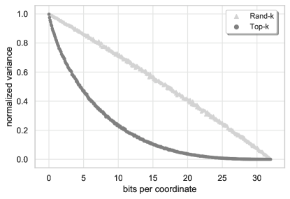
Figure 1: The comparison of Top-$k$ and Rand-$k$ sparsifiers with respect to normalized variance and the number of encoding bits used for each coordinate on average. Each point/marker represents a single $d=10^{4}$ dimensional vector drawn form Gaussian distribution and then compressed by the specified operator. Each curve was obtained by varying the free parameter $k\in\{1,2,\dots,d\}$. Plots for different $d$ look very similar. Notice that, for random sparsification the normalized variance is perfectly linear with respect to the number of bit per coordinate. Letting $b$ be the total number of bits to encode the compressed vector (say in binary32 system), the normalized variance produced by random sparsifier is almost $1-\tfrac{\nicefrac{{b}}{{d}}}{32}$. However, greedy sparsifier achieves exponentially lower variance $\approx 0.86^{\nicefrac{{b}}{{d}}}$ utilizing the same amount of bits.

First, we compare the savings $s_{top}^{k}$ and $s_{rnd}^{k}$ of these compressions. For random sparsification, we have

$${{\rm E}}\left[s_{rnd}^{k}(x)\right]=k\cdot(\sigma^{2}+\mu^{2}),$$

where $\mu$ and $\sigma^{2}$ are the mean and variance of the Gaussian distribution. For computing ${{\rm E}}\left[s_{top}^{k}(x)\right]$, we use the probability density function of $k$-th order statistics (see (31) or (2.2.2) of (Arnold et al., 1992)). Table 4 shows that Top-$3$ and Top-$5$ sparsifiers “save” $3\times$–$40\times$ more information in expectation and the factor grows with the dimension.

Next we compare normalized variances $\frac{\omega_{top}^{k}(x)}{\left\|x\right\|_{2}^{2}}$ and $\frac{\omega_{rnd}^{k}(x)}{\left\|x\right\|_{2}^{2}}$ for randomly generated Gaussian vectors. In an attempt to give a dimension independent comparison, we compare them against the average number of encoding bits per coordinate, which is quite stable with respect to the dimension. Figure 1 reveals the superiority of greedy sparsifier against the random one.

Practical distribution.

We obtained various gradient distributions via logistic regression (mushrooms LIBSVM dataset) and least squares. We used the sklearn package and built Gaussian smoothing of the practical gradient density. The second moments, i.e. energy “saving”, were already calculated from it by formula for density function of $k$-order statistics, see Appendix A.4 or (Arnold et al., 1992). We conclude experiments for Top-5 and Rand-5, see Figure 2 for details.

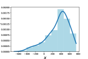
(a)
$s_{rnd}^{5}=9\cdot 10^{5}$,
$s_{top}^{5}=28\cdot 10^{5}$

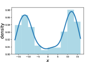
(b)
$s_{rnd}^{5}=624$,
$s_{top}^{5}=1357$

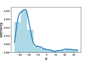
(c)
$s_{rnd}^{5}=11921$,
$s_{top}^{5}=23488$

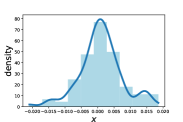
(d)
$s_{rnd}^{5}=2\cdot 10^{-4}$,
$s_{top}^{5}=17\cdot 10^{-4}$

Figure 2: Calculations of the Rand-5 and Top-5 energy “saving” for practical gradient distributions ((a),(b),(c): quadratic problem, (d): logistic regression). The results of Top-5 are 3–5$\times$ better.

4.2 New compressor: Top-$k$ combined with dithering

In Section 2.2 we gave a new biased compression operator (see (16)), where we combined Top-$k$ sparsification operator (see (11)) with the general exponential dithering (see (14)). Consider the composition operator with natural dithering, i.e., with base $b=2$. We showed that it belongs to $\mathbb{B}^{1}(\frac{k}{d},\frac{9}{8})$, $\mathbb{B}^{2}(\frac{k}{d},\frac{9}{8})$ and $\mathbb{B}^{3}(\frac{9d}{8k})$. Figure 3 empirically confirms that it attains the lowest compression parameter $\delta\geq 1$ among all other known compressors (see (5)). Furthermore, the iteration complexity ${\cal O}\left(\delta\tfrac{L}{\mu}\log\tfrac{1}{\varepsilon}\right)$ of CGD for ${\cal C}\in\mathbb{B}^{3}(\delta)$ implies that it enjoys fastest convergence.

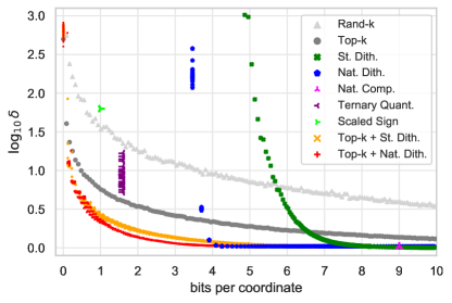
Figure 3: Comparison of various compressors (with and without free design parameters) with respect to the parameter $\delta\geq 1$ in $\log_{10}-$scale and the number of encoding bits used for each coordinate on average. Each point/marker represents a single $d=10^{4}$ dimensional vector $x$ drawn from Gaussian distribution and then compressed by the specified operator. Each curve was obtained by varying free parameters ($k\in\{1,2,\dots,d\}$ for sparsifiers, $s\geq 1$ for ditherings) of the specified compressor. Parameter-free compressors, such as ternary quantization and natural compression, have fixed communication budgets which explains the vertical arrangements of the points.

5 Distributed Setting

We now focus attention on a distributed setup with $n$ machines, each of which owns non-iid data defining one loss function $f_{i}$. Our goal is to minimize the average loss:

$$\min\limits_{x\in\mathbb{R}^{d}}\left\{f(x)\coloneqq\frac{1}{n}\sum\limits_{i=1}^{n}f_{i}(x)\right\}.$$ (17)

5.1 Distributed CGD with unbiased compressors

Perhaps the most straightforward extension of CGD to the distributed setting is to consider the method

$$x^{k+1}=x^{k}-\eta\frac{1}{n}\sum\limits_{i=1}^{n}{\cal C}^{k}_{i}(\nabla f_{i}(x^{k})).$$ (DCGD)

Indeed, for $n=1$ this method reduces to CGD. For unbiased compressors belonging to $\mathbb{U}(\zeta)$, this method converges under suitable assumptions on the functions. For instance, if $f_{i}$ are $L$-smooth and $f$ is $\mu$-strongly convex, then as long as the stepsize is chosen appropriately, the method converges to a ${\cal O}\left(\frac{\eta D(\zeta-1)}{\mu n}\right)$ neighborhood of the (necessarily unique) solution $x^{\star}$ with the linear rate

$${\cal O}\left(\left(\frac{L}{\mu}+\frac{L(\zeta-1)}{\mu n}\right)\log\frac{1}{\epsilon}\right),$$

where $D\coloneqq\frac{1}{n}\sum\limits_{i=1}^{n}\left\|\nabla f_{i}(x^{\star})\right\|_{2}^{2}$ (Gorbunov et al., 2020a). In particular, in the overparameterized setting when $D=0$, the method converges to the exact solution, and does so at the same rate as GD as long as $\zeta={\cal O}(n)$. These results hold even if a regularizer is considered, and a proximal step is added to DCGD. Moreover, as shown by Mishchenko et al. (2019) and Horváth et al. (2019b), a variance reduction technique can be devised to remove the neighborhood convergence and replace it by convergence to $x^{\star}$, at the negligible additional cost of ${\cal O}((\zeta-1)\log\frac{1}{\epsilon})$.

5.2 Failure of DCGD with biased compressors

However, as we now demonstrate by giving some counter-examples, DCGD may fail if the compression operators are allowed to be biased. In the first example below, DCGD used with the Top-1 compressor diverges at an exponential rate.

Example 1

Consider $n=d=3$ and define

$$f_{1}(x)=\langle a,x\rangle^{2}+\frac{1}{4}\left\|x\right\|_{2}^{2},\qquad f_{2}(x)=\langle b,x\rangle^{2}+\frac{1}{4}\left\|x\right\|_{2}^{2},\qquad f_{3}(x)=\langle c,x\rangle^{2}+\frac{1}{4}\left\|x\right\|_{2}^{2},$$

where $a=(-3,2,2)$, $b=(2,-3,2)$ and $c=(2,2,-3)$. Let the starting iterate be $x^{0}=(t,t,t)$, where $t>0$. Then

$$\nabla f_{1}(x^{0})=\frac{t}{2}(-11,9,9),\qquad\nabla f_{2}(x^{0})=\frac{t}{2}(9,-11,9),\qquad\nabla f_{3}(x^{0})=\frac{t}{2}(9,9,-11).$$

Using the Top-1 compressor, we get ${\cal C}(\nabla f_{1}(x^{0}))=\frac{t}{2}(-11,0,0)$, ${\cal C}(\nabla f_{2}(x^{0}))=\frac{t}{2}(0,-11,0)$ and ${\cal C}(\nabla f_{3}(x^{0}))=\frac{t}{2}(0,0,-11)$. The next iterate of DCGD is

$$x^{1}=x^{0}-\eta\frac{1}{3}\sum_{i=1}^{3}{\cal C}(\nabla f_{i}(x^{0}))=\left(1+\frac{11\eta}{6}\right)x^{0}.$$

Repeated application gives

$$x^{k}=\left(1+\frac{11\eta}{6}\right)^{k}x^{0}.$$

Since $\eta>0$, the entries of $x^{k}$ diverge exponentially fast to $+\infty$.

The above counter-example can be extended to the case of Top-$d_{1}$ when $d_{1}<\left\lceil\frac{d}{2}\right\rceil$.

Example 2

Fix the dimension $d\geq 3$ and let $n=\binom{d}{d_{1}}$ be the number of nodes, where $d_{1}<\left\lceil\frac{d}{2}\right\rceil$ and $d_{2}=d-d_{1}>d_{1}$. Choose positive numbers $b,\;c>0$ such that

$$-bd_{1}+cd_{2}=1,\;b>c+1.$$

One possible choice could be $b=d_{2}+\frac{d_{2}}{d_{1}},\;c=d_{1}+\frac{1}{d_{2}}+1$. Define vectors $a_{j}\in\mathbb{R}^{d},\;j\in[n]$ via

$$a_{j}=\sum_{i\in I_{j}}(-b)e_{i}+\sum_{i\in[d]\setminus I_{j}}ce_{i},$$

where sets $I_{j}\subset[d],\;j\in[n]$ are all possible $d_{1}$-subsets of $[d]$ enumerated in some way. Define

$$f_{j}(x)=\langle a_{j},x\rangle^{2}+\frac{1}{2}\left\|x\right\|_{2}^{2},\quad j\in[n]$$

and let the initial point be $x^{0}=te,\;t>0$, where $e=\sum_{i=1}^{d}e_{i}$ is the vector of all $1$s. Then

$$\nabla f_{j}(x^{0})=2\langle a_{j},x^{0}\rangle\cdot a_{j}+x^{0}=2t(-bd_{1}+cd_{2})\cdot a_{j}+te=t(2a_{j}+e).$$

Since $|2(-b)+1|>|2c+1|$, then using the Top-$d_{1}$ compressor, we get

$${\cal C}(\nabla f_{j}(x^{0}))=-t(2b-1)\sum_{i\in I_{j}}e_{i}.$$

Therefore, the next iterate of DCGD is

$$x^{1} = x^{0}-\eta\frac{1}{n}\sum_{j=1}^{n}{\cal C}(\nabla f_{j}(x^{0}))=x^{0}+\frac{\eta t(2b-1)}{n}\sum_{j=1}^{n}\sum_{i\in I_{j}}e_{i}$$

$$= x^{0}+\frac{\eta(2b-1)}{n}\binom{d}{d_{1}-1}x^{0}=\left(1+\frac{\eta(2b-1)d_{1}}{d_{2}+1}\right)x^{0},$$

which implies

$$x^{k}=\left(1+\frac{\eta(2b-1)d_{1}}{d_{2}+1}\right)^{k}x^{0}.$$

Since $\eta>0$ and $b>1$, the entries of $x^{k}$ diverge exponentially fast to $+\infty$.

Finally, we present more general counter-example with different type of failure for DCGD when non-randomized compressors are used.

Example 3

Let ${\cal C}\colon\mathbb{R}^{d}\to\mathbb{R}^{d}$ be any deterministic mapping for which there exist vectors $v_{1},v_{2},\dots,v_{m}\in\mathbb{R}^{d}$ such that

$$\sum_{i=1}^{m}v_{i}\neq 0,\qquad\text{and}\qquad\sum_{i=1}^{m}{\cal C}(v_{i})=0.$$ (18)

Consider the distributed optimization problem (17) with $n=m$ devices and with the following strongly convex loss functions

$$f_{i}(x)=\left\langle v_{i},x\right\rangle+\frac{1}{2}\|x\|^{2},\quad i\in[m].$$

Then $\nabla f_{i}(x)=v_{i}+x$ and $\nabla f(x)=\frac{1}{n}\sum_{i=1}^{n}v_{i}+x$. Hence, the optimal point $x^{*}=-\frac{1}{n}\sum_{i=1}^{n}v_{i}\neq 0$. However, it can be easily checked that, with initialization $x_{0}=0$, we have

$$x^{1}=x^{0}-\gamma\frac{1}{n}\sum_{i=1}^{n}{\cal C}(\nabla f_{i}(x^{0}))=x^{0}-\gamma\frac{1}{n}\sum_{i=1}^{n}{\cal C}(v_{i}+x^{0})=x^{0}.$$

Thus, when initialized at $x_{0}=0$, not only DCGD does not converge to the solution $x^{*}\neq 0$, it remains stuck at the same initial point for all iterates, namely $x^{k}=x^{0}=0$ for all $k\geq 1$.

Condition (18) can be easily satisfied for specific biased compressors. For instance, Top-$1$ satisfies (18) with $v_{1}=\left[\begin{smallmatrix}1\\ 4\end{smallmatrix}\right]$, $v_{2}=\left[\begin{smallmatrix}-1\\ -2\end{smallmatrix}\right]$, $v_{3}=\left[\begin{smallmatrix}1\\ -2\end{smallmatrix}\right]$.

The above examples suggests that one needs to devise a different approach to solving the distributed problem (17) with biased compressors. We resolve this problem by employing a memory feedback mechanism.

5.3 Error Feedback

We show that distributed version of Distributed SGD wtih Error-Feedback (Karimireddy et al., 2019b), displayed in Algorithm 1, is able to resolve the issue. Moreover, this algorithm allows for the computation of stochastic gradients. Each step starts with all machines $i$ in parallel computing a stochastic gradient $g_{i}^{k}$ of the form

$$g_{i}^{k}=\nabla f_{i}(x^{k})+\xi_{i}^{k},$$ (19)

where $\nabla f_{i}(x^{k})$ is the true gradient, and $\xi_{i}^{k}$ is a stochastic error. Then, this is multiplied by a stepsize $\eta^{k}$ and added to the memory/error-feedback term $e_{i}^{k}$, and subsequently compressed. The compressed messages are communicated and aggregated. The difference of message we wanted to send and its compressed version becomes stored as $e_{i}^{k+1}$ for further correction in the next communication round. The output $\overline{x}^{K}$ is an ergodic average of the form

$$\overline{x}^{K}\coloneqq\frac{1}{W^{K}}\sum_{k=0}^{K}w^{k}x^{k},\qquad W^{K}\coloneqq\sum_{k=0}^{K}w^{k}.$$ (20)

  Parameters: Compressors ${\cal C}_{i}^{k}\in\mathbb{B}^{3}(\delta)$; Stepsizes $\{\eta^{k}\}_{k\geq 0}$; Iteration count $K$

Initialization: Choose $x^{0}\in\mathbb{R}^{d}$ and $e_{i}^{0}=0$ for all $i$

  for $k=0,1,2,\ldots,K$  do

     Server sends $x^{k}$ to all $n$ machines

     All machines in parallel perform these updates:

$$\tilde{g}_{i}^{k}={\cal C}^{k}_{i}(e_{i}^{k}+\eta^{k}g_{i}^{k})$$ (21)

$$e_{i}^{k+1}=e_{i}^{k}+\eta^{k}g_{i}^{k}-\tilde{g}_{i}^{k}$$ (22)

     Each machine $i$ sends $\tilde{g}_{i}^{k}$ to the server

     Server performs aggregation:

$$x^{k+1}=x^{k}-\frac{1}{n}\sum\limits_{i=1}^{n}\tilde{g}_{i}^{k}$$ (23)

  end for

Output: Weighted average of the iterates: $\overline{x}^{K}$ (20)

Algorithm 1 Distributed SGD with Biased Compression and Error Feedback

5.4 Complexity theory

We assume the stochastic error $\xi_{i}^{k}$ in (19) satisfies the following condition.

Assumption 1

Stochastic error $\xi_{i}^{k}$ is unbiased, i.e. ${{\rm E}}\left[\xi_{i}^{k}\right]=0$, and for some constants $B,C\geq 0$

$${{\rm E}}\left[\left\|\xi_{i}^{k}\right\|_{2}^{2}\right]\leq B\left\|\nabla f_{i}(x^{k})\right\|_{2}^{2}+C,\qquad\forall i\in[n],k\geq 0.$$ (24)

Note that this assumption is much weaker than the bounded variance assumption (i.e., ${{\rm E}}\left[\left\|\xi_{i}^{k}\right\|_{2}^{2}\right]\leq C$) and bounded gradient assumption (i.e., ${{\rm E}}\left[\left\|g_{i}^{k}\right\|_{2}^{2}\right]\leq C$). We can now state the main result of this section. To the best of our knowledge, this was an open problem: we are not aware of any convergence results for distributed optimization that tolerate general classes of biased compression operators and have reasonable assumptions on the stochastic gradient.

Theorem 21 (Convergence guarantees for Algorithm 1)

Let $\{x^{k}\}_{k\geq 0}$ denote the iterates of Algorithm 1 for solving problem (1), where each $f_{i}$ is $L$-smooth and $\mu$-strongly convex. Let $x^{\star}$ be the minimizer of $f$ and let $f^{\star}\coloneqq f(x^{\star})$ and

$$D\coloneqq\frac{1}{n}\sum_{i=1}^{n}\left\|\nabla f_{i}(x^{\star})\right\|_{2}^{2}.$$

Assume the compression operator used by all nodes is in $\mathbb{B}^{3}(\delta)$. Then we have the following convergence rates under three different stepsize and iterate weighting regimes:

• ${\cal O}(\frac{1}{k})$ stepsizes & ${\cal O}(k)$ weights. Let, for all $k\geq 0$, the stepsizes and weights be set as $\eta^{k}=\frac{4}{\mu(\kappa+k)}$ and $w^{k}=\kappa+k$, respectively, where $\kappa=\frac{56(2\delta+B)L}{\mu}$. Then

  $$\boxed{{{\rm E}}\left[f(\bar{x}^{K})\right]-f^{\star}={\cal O}\left(\frac{A_{1}}{K^{2}}+\frac{A_{2}}{K}\right)}\,,$$

  where $A_{1}\coloneqq\frac{L^{2}(2\delta+B)^{2}}{\mu}\left\|x^{0}-x^{\star}\right\|_{2}^{2}$ and $A_{2}\coloneqq\frac{C\left(1+\nicefrac{{1}}{{n}}\right)+D\left(\nicefrac{{2B}}{{n}}+3\delta\right)}{\mu}$.

• ${\cal O}(1)$ stepsizes & ${\cal O}(e^{-k})$ weights. Let, for all $k\geq 0$, the stepsizes and weights be set as $\eta^{k}=\eta$ and $w^{k}=(1-\mu\eta/2)^{-(k+1)}$, respectively, where $\eta\leq\frac{1}{14(2\delta+B)L}$. Then

  $$\boxed{{{\rm E}}\left[f(\bar{x}^{K})\right]-f^{\star}=\tilde{\cal O}\left(A_{3}\exp\left[-\frac{K}{A_{4}}\right]+\frac{A_{2}}{K}\right)}\,,$$

  where $A_{3}\coloneqq L(2\delta+B)\left\|x^{0}-x^{\star}\right\|_{2}^{2}$ and $A_{4}\coloneqq\frac{28L(2\delta+B)}{\mu}$.

• ${\cal O}(1)$ stepsizes & equal weights. Let, for all $k\geq 0$, the stepsizes and weights be set as $\eta^{k}=\eta$ and $w^{k}=1$, respectively, where $\eta\leq\frac{1}{14(2\delta+B)L}$. Then

  $$\boxed{{{\rm E}}\left[f(\bar{x}^{K})\right]-f^{\star}={\cal O}\left(\frac{A_{3}}{K}+\frac{A_{5}}{\sqrt{K}}\right)}\,,$$

  where $A_{5}\coloneqq\sqrt{C\left(1+\nicefrac{{1}}{{n}}\right)+D\left(\nicefrac{{2B}}{{n}}+3\delta\right)}\left\|x^{0}-x^{\star}\right\|_{2}$.

Let us make a few observations on these results. First, Algorithm 1 employing general biased compressors and error feedback mechanism indeed resolves convergence issues of DCGD method by converging the optimal solution $x^{*}$. Second, note that the choice of stepsizes $\eta^{k}$ and weights $w^{k}$ leading to convergence is not unique and several schedules are feasible. Third, all the rates are sublinear and based on the second rate (ii) above, linear convergence is guaranteed if $C=D=0$. Based on (24), one setup when the condition $C=0$ holds is when all devices compute full local gradients (i.e., $g_{i}^{k}=\nabla f_{i}(x^{k})$). Furthermore, the condition $D=0$ is equivalent to $\nabla f_{i}(x^{\star})=0$ for all $i\in[n]$, which is typically satisfied for over-parameterized models. Lastly, under these two assumptions (i.e., devices can compute full local gradients and the model is over-parameterized), we show that distributed SGD method with error feedback converges with the same ${\cal O}\left(\delta\frac{L}{\mu}\log\frac{1}{\epsilon}\right)$ linear rate as single node CGD algorithm. To the best of our knowledge, this was the first regime where distributed first order method with biased compression is guaranteed to converge linearly.

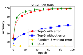
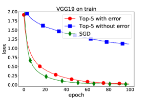
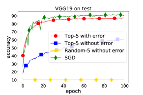
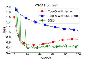
Figure 4: Training/Test loss and accuracy for VGG19 on CIFAR10 distributed among $4$ nodes for $4$ different compression operators.

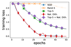
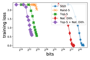
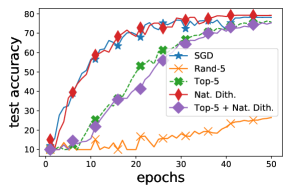
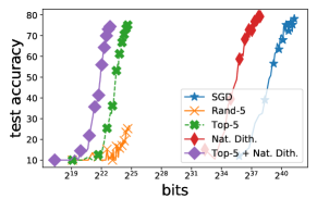
Figure 5: Training loss and test accuracy for VGG11 on CIFAR10 distributed among $4$ nodes for $5$ different compression operators.

6 Experiments

In Sections 6.1–6.4, we present our experiments, which are primarily focused on supporting our theoretical findings. Therefore, we simulate these experiments on one machine which enable us to do rapid direct comparisons against the prior methods. In more details, we use the machine with 24 Intel(R) Xeon(R) Gold 6146 CPU @ 3.20GHz cores and GPU GeForce GTX 1080 Ti. Section 6.5 is devoted to real experiments with a large model and big data. For these experiments, we use a computational cluster with 10 GPUs Tesla T4. We implement all methods in Python 3.7 using Pytorch Paszke et al. (2019).

6.1 Lower empirical variance induced by biased compressors during deep network training

Motivated by our theoretical results in Section 4, we show that similar behaviour can be seen in the empirical variance of gradients. We run 2 sets of experiments with Resnet18 on CIFAR10 dataset. In Figure 6, we display empirical variance, which is obtained by running a training procedure with specific compression. We compare unbiased and biased compressions with the same communication complexities–deterministic with classic/unbiased ${\cal C}_{\rm nat}$ and Top-$k$ with Rand-$k$ with $k$ to be $\nicefrac{{1}}{{5}}$ of coordinates. One can clearly see, that there is a gap in empirical variance between biased and unbiased methods, similar to what we have shown in theory, see Section 4.

6.2 Error-feedback is needed in distributed training with biased compression

The next experiment shows the need of error-feedback for methods with biased compression operators. Based on Example 1, error feedback is necessary to prevent divergence from the optimal solution. Figure 4 displays training/test loss and accuracy for VGG19 on CIFAR10 with data equally distributed among $4$ nodes. We use plain SGD with a default step size equal to $0.01$ for all methods, i.e. Top-$5$ with and without error feedback, Rand-$5$ and no compression. As suggested by the counterexample, not using error feedback can really hurt the performance when biased compressions are used. Also note, that performance of Rand-$5$ is significantly worse than Top-$5$.

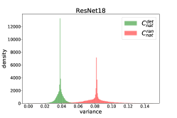
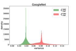
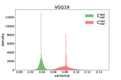
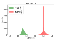
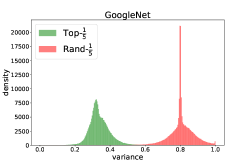
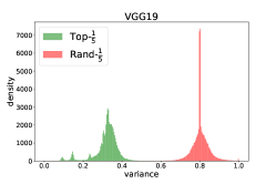
Figure 6: Comparison of empirical variance $\left\|{\cal C}(x)-x\right\|_{2}^{2}/\left\|x\right\|_{2}^{2}$ during training procedure for two pairs of method– deterministic with classic/unbiased ${\cal C}_{\rm nat}$ and Top-$k$ with Rand-$k$ with Top-$\nicefrac{{1}}{{5}}$ of coordinates. Both of the plots were produced using ResNet18, GoogleNet, and VGG19 on CIFAR10 dataset.

6.3 Top-$k$ mixed with natural dithering saves in communication significantly

Next, we experimentally show the superiority of our newly proposed compressor–Top-$k$ combined with natural dithering. We compare this against current state-of-the-art for low bandwidth approach Top-$k$ for some small $k$. In Figure 5, we plot comparison of $5$ methods–Top-$k$, Rand-$k$, natural dithering, Top-$k$ combined with natural dithering and plain SGD. We use $2$ levels with infinity norm for natural dithering and $k=5$ for sparsification methods. For all the compression operators, we train VGG11 on CIFAR10 with plain SGD as an optimizer and default step size equal to $0.01$. We can see that adding natural dithering after Top-$k$ has the same effect as the natural dithering comparing to no compression, which is a significant reduction in communications without almost no effect on convergence or generalization. Using this intuition, one can come to the conclusion that Top-$k$ with natural dithering is the best compression operator for any bandwidth, where we adjust to given bandwidth by adjusting $k$. This exactly matches with our previous theoretical variance estimates displayed in Figure 3.

6.4 Theoretical behavior predicts the actual performance in practice

In the next experiment, we provide numerical results to further show that our predicted theoretical behavior matches the actual performance observed in practice. We run two regression experiments optimized by gradient descent with step-size $\eta=\frac{1}{L}$. We use a slightly adjusted version of Theorem 19 with adaptive step-sizes, namely

$$\frac{f(x^{k})-f(x^{\star})}{f(x^{0})-f(x^{\star})}\leq\prod\limits_{i=1}^{k}\left(1-\frac{\mu}{L\delta_{i}}\right),$$

where

$$1-\frac{1}{\delta_{i}}=\frac{\left\|{\cal C}(\nabla f(x^{i}))-\nabla f(x^{i})\right\|_{2}^{2}}{\left\|\nabla f(x^{i})\right\|_{2}^{2}}.$$

Note that this is the direct consequence of our analysis. We apply this property to display the theoretical convergence. In the first experiment depicted in Figure 7, we randomly generate random square matrix $A$ of dimension $100$ where it is constructed in the following way: we sample random diagonal matrix $D$, which elements are independently sampled from the uniform distribution $(1,10)$, $(1,100)$, and $(1,1000)$, respectively. $A$ is then constructed using $Q^{\top}DQ$, where $P=QR$ is a random matrix and $QR$ is obtained using QR-decomposition. The label $y$ is generated the same way from the uniform distribution $(0,1)$. The optimization objective is then

$$\min_{x\in\mathbb{R}^{d}}x^{\top}Ax-y^{\top}x.$$

For the second experiment shown in Figure 8, we run standard linear regression on two scikit-learn datasets–Boston and Diabetes–and applied data normalization as the preprocessing step.

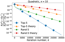
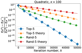
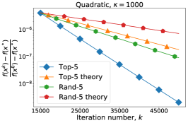
Figure 7: Theoretical vs. Practical Convergence of Compressed Gradient Descent on Quadratics problem with different condition number $\kappa$ for Top-5 and Rand-5 compression operators.

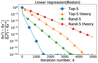
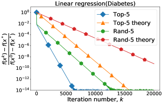
Figure 8: Theoretical vs. Practical Convergence of Compressed Gradient Descent on Linear Regression problem for Boston and Diabetes datasets with Top-5 and Rand-5 compression operators.

Looking into Figures 7 and 8, one can clearly see that as predicted by our theory, biased compression with less empirical variance leads to better convergence in practice and the gap almost matches the improvement.

6.5 Transformer training

In the last experiment, we work with a real big model. In particular, we train ALBERT-large (Lan et al., 2020) (18M parameters) with layer sharing on a combination of Bookcorpus (Zhu et al., 2015) and Wikipedia (Devlin et al., 2018) datasets. We use the same optimizer (LAMB) and the same tuning for it as in the original paper (Lan et al., 2020). Our goal is to find an unbiased and biased operators such that we maximize the improvement in terms of communication cost without losing much in terms of training quality. In this case, we include in the communication cost both the time to perform the communication round and the time to perform the compression and decompression operations. It is important to note that we do not compress packages with gradients corresponding to LayerNorm scales, but this is less than $1$ percent of the whole package. Among unbiased compressors, we try natural compression (Section 2.2 (g)) and random sparsification (Section 2.2 (a)). The best result is shown by natural compression, which compresses the packages by a factor of $4$. The Rand-$25$ operator (which also compresses the information by a factor of $4$) performs much worse even with the use of the error feedback technique. For communications with natural compression, we use the classical allreduce procedure. Among unbiased compressors, we try Top-$k$ sparsification (Section 2.2 (d)) and Power compression (Vogels et al., 2019). The best result is shown by Power compression with the rank parameter $r{=}8$ and the error feedback. The organization of communications (allreduce procedures) occurs as in the original paper (Vogels et al., 2019). We measure how the training loss changes (Figure 9) as well as at the end of training we evaluate the final performance for each model on several popular tasks from (Wang et al., 2018) (Table 5). The results show that the use of biased compression can significantly reduce the communication time cost compared to uncompressed and even unbiased compression setups. At the same time, the quality of the training does not drop much.

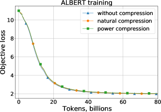
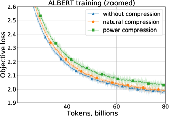
Figure 9: Training objective value for ALBERT-large with different compression operators.

Setup	Avg time	CoLA	MNLI	MRPC	QNLI	QQP	RTE	SST2	STS-B
Without compression	9.62 $\pm$ 0.03	46.2	81.1	82.5	87.9	88.0	66.3	85.1	88.0
Natural compression	4.05 $\pm$ 0.05	48.3	81.0	87.5	87.8	84.4	63.2	87.8	86.9
Power compression	1.04 $\pm$ 0.04	42.4	80.3	85.1	88.2	85.3	46.3	88.0	87.4

Table 5: Comparison of average time per one communication round and downstream evaluation scores on GLUE benchmark tasks.

Appendix

Appendix A Basic Facts and Inequalities

A.1 Strong convexity

Function $f$ is strongly convex on $\mathbb{R}^{d}$ when it is continuously differentiable and there is a constant $\mu>0$ such that the following inequality holds:

$$\frac{\mu}{2}\left\|x-y\right\|_{2}^{2}\leq f(x)-f(y)-\langle\nabla f(y),x-y\rangle,\qquad\forall x,y\in\mathbb{R}^{d}.$$ (25)

A.2 Smoothness

Function $f$ is called $L$-smooth in $\mathbb{R}^{d}$ with $L>0$ when it is differentiable and its gradient is $L$-Lipschitz continuous, i.e.

$$\left\|\nabla f(x)-\nabla f(y)\right\|_{2}\leq L\left\|x-y\right\|_{2},\qquad\forall x,y\in\mathbb{R}^{d}.$$

If convexity is assumed as well, then the following inequalities hold:

$$\frac{1}{2L}\left\|\nabla f(x)-\nabla f(y)\right\|_{2}^{2}\leq f(x)-f(y)-\langle\nabla f(y),x-y\rangle,\qquad\forall x,y\in\mathbb{R}^{d}$$ (26)

By plugging $y=x^{*}$ to (26), we get

$$\left\|\nabla f(x)\right\|_{2}^{2}\leq 2L(f(x)-f(x^{*})),\qquad\forall x\in\mathbb{R}^{d}.$$ (27)

A.3 Useful inequalities

For all $a,b,x_{1},\ldots,x_{n}\in\mathbb{R}^{d}$ and $\xi>0$ the following inequalities holds:

$$2\langle a,b\rangle\leq\frac{\left\|a\right\|_{2}^{2}}{\xi}+\xi\left\|b\right\|_{2}^{2},$$ (28)

$$\left\|a+b\right\|_{2}^{2}\leq\left(1+\frac{1}{\xi}\right)\left\|a\right\|_{2}^{2}+(1+\xi)\left\|b\right\|_{2}^{2},$$ (29)

$$\left\|\sum\limits_{i=1}^{n}x_{i}\right\|_{2}^{2}\leq n\cdot\sum\limits_{i=1}^{n}\left\|x_{i}\right\|_{2}^{2}.$$ (30)

A.4 Facts from order statistics

For i.i.d. samples $x_{1},x_{2},\ldots,x_{d}$ from an absolutely continuous distribution with probability density function $\phi$ and cumulative distribution function $\Phi$ let $x_{(1)}\leq x_{(2)}\leq\dots\leq x_{(d)}$ be the order statistics obtained by arranging samples in increasing order of magnitude. Then the following expressions give the density function of $x_{(i)}$ ($1\leq i\leq d$)

$$\phi_{x_{(i)}}(u)=\frac{d!}{(i-1)!(d-i)!}\{\Phi(u)\}^{i-1}\{1-\Phi(u)\}^{n-i}\phi(u),\quad-\infty<u<\infty,$$ (31)

and the joint density function of all $d$ order statistics

$$\phi_{x_{(1)},\dots,x_{(d)}}(u_{1},\dots,u_{d})=d!\prod\limits_{i=1}^{d}\phi(u_{i}),\quad-\infty<u_{1}\leq\dots\leq u_{d}<\infty.$$ (32)

Appendix B Proofs for Section 2.2

B.1 Proof of Lemma 8: Unbiased Random Sparsification

From the definition of $k$-nice sampling we have $p_{i}\coloneqq\operatorname{Prob}\left(i\in S\right)=\tfrac{k}{d}$. Hence

$${{\rm E}}\left[{\cal C}(x)\right] =\frac{d}{k}{{\rm E}}\left[\sum_{i\in S}x_{i}e_{i}\right]=\frac{d}{k}\sum_{i=1}^{d}p_{i}x_{i}e_{i}=\sum_{i=1}^{d}x_{i}e_{i}=x,$$

$${{\rm E}}\left[\left\|{\cal C}(x)\right\|_{2}^{2}\right] =\frac{d^{2}}{k^{2}}{{\rm E}}\left[\sum_{i\in S}x_{i}^{2}\right]=\frac{d^{2}}{k^{2}}\sum_{i=1}^{d}p_{i}x_{i}^{2}=\frac{d}{k}\sum_{i=1}^{d}x_{i}^{2}=\frac{d}{k}\left\|x\right\|_{2}^{2},$$

which implies ${\cal C}\in\mathbb{U}(\tfrac{d}{k})$.

B.2 Proof of Lemma 9: Biased Random Sparsification

Let $S\subseteq[d]$ be a proper sampling with probability vector $p=(p_{1},\dots,p_{d})$, where $p_{i}\coloneqq\operatorname{Prob}(i\in S)>0$ for all $i$. Then

$${{\rm E}}\left[{\cal C}(x)\right]=\mathbf{Diag}\left(p\right)x=\sum_{i=1}^{d}p_{i}x_{i}e_{i}\quad\text{and}\quad{{\rm E}}\left[\left\|{\cal C}(x)\right\|_{2}^{2}\right]=\sum_{i=1}^{d}p_{i}x_{i}^{2}.$$

Letting $q\coloneqq\min_{i}p_{i}$, we get

$$q\left\|x\right\|_{2}^{2}\leq\sum\limits_{i=1}^{d}p_{i}x_{i}^{2}={{\rm E}}\left[\left\|{\cal C}(x)\right\|_{2}^{2}\right]=\left\langle{{\rm E}}\left[{\cal C}(x)\right],x\right\rangle.$$

So, ${\cal C}\in\mathbb{B}^{1}(q,1)$ and ${\cal C}\in\mathbb{B}^{2}(q,1)$. For the third class, note that

$${{\rm E}}\left[\left\|{\cal C}(x)-x\right\|_{2}^{2}\right]=\sum\limits_{i=1}^{d}(1-p_{i})x_{i}^{2}\leq(1-q)\left\|x\right\|_{2}^{2}.$$

Hence, ${\cal C}\in\mathbb{B}^{3}(\tfrac{1}{q})$.

B.3 Proof of Lemma 10: Adaptive Random Sparsification

From the definition of the compression operator, we have

$${{\rm E}}\left[\left\|{\cal C}(x)\right\|_{2}^{2}\right] ={{\rm E}}\left[x_{i}^{2}\right]=\sum\limits_{i=1}^{d}\frac{|x_{i}|}{\left\|x\right\|_{1}}x_{i}^{2}=\frac{\left\|x\right\|_{3}^{3}}{\left\|x\right\|_{1}},$$

$${{\rm E}}\left[\langle{\cal C}(x),x\rangle\right] ={{\rm E}}\left[x_{i}^{2}\right]=\frac{\left\|x\right\|_{3}^{3}}{\left\|x\right\|_{1}},$$

whence $\beta=1$. Furthermore, by Chebychev’s sum inequality, we have

$$\tfrac{1}{d^{2}}\left\|x\right\|_{1}\left\|x\right\|_{2}^{2}=\left(\sum\limits_{i=1}^{d}\tfrac{1}{d}|x_{i}|\right)\left(\sum\limits_{i=1}^{d}\tfrac{1}{d}x_{i}^{2}\right)\leq\sum\limits_{i=1}^{d}\tfrac{1}{d}|x_{i}|x_{i}^{2}=\tfrac{1}{d}\left\|x\right\|_{3}^{3},$$

which implies that $\alpha=\frac{1}{d},\,\delta=d$. So, ${\cal C}\in\mathbb{B}^{1}(\frac{1}{d},1)$, ${\cal C}\in\mathbb{B}^{2}(\frac{1}{d},1)$, and ${\cal C}\in\mathbb{B}^{3}(d)$.

B.4 Proof of Lemma 11: Top-$k$ sparsification

Clearly, $\left\|{\cal C}(x)\right\|_{2}^{2}=\sum_{i=d-k+1}^{d}x_{(i)}^{2}$ and $\left\|{\cal C}(x)-x\right\|_{2}^{2}=\sum_{i=1}^{d-k}x_{(i)}^{2}$. Hence

$$\frac{k}{d}\left\|x\right\|_{2}^{2}\leq\left\|{\cal C}(x)\right\|_{2}^{2}=\langle{\cal C}(x),x\rangle\leq\left\|x\right\|_{2}^{2},\quad\left\|{\cal C}(x)-x\right\|_{2}^{2}\leq\left(1-\frac{k}{d}\right)\left\|x\right\|_{2}^{2}.$$

So, ${\cal C}\in\mathbb{B}^{1}(\frac{k}{d},1)$, ${\cal C}\in\mathbb{B}^{2}(\frac{k}{d},1)$, and ${\cal C}\in\mathbb{B}^{3}(\frac{d}{k})$.

B.5 Proof of Lemma 12: General Unbiased Rounding

The unbiasedness follows immediately from the definition (12)

$${{\rm E}}\left[{\cal C}(x)\right]=\sum_{i=1}^{d}{{\rm E}}\left[{\cal C}(x)_{i}\right]e_{i}=\sum_{i=1}^{d}\operatorname{sign}(x_{i})\left(a_{k}\frac{a_{k+1}-|x_{i}|}{a_{k+1}-a_{k}}+a_{k+1}\frac{|x_{i}|-a_{k}}{a_{k+1}-a_{k}}\right)e_{i}=\sum_{i=1}^{d}x_{i}e_{i}=x.$$ (33)

Since the rounding compression operator ${\cal C}$ applies to each coordinate independently, without loss of generality we can consider the compression of scalar values $x=t>0$ and show that ${{\rm E}}\left[{\cal C}(t)^{2}\right]\leq\zeta\cdot t^{2}$. From the definition we compute the second moment as follows

$${{\rm E}}\left[\mathcal{C}(t)^{2}\right]=a_{k}^{2}\frac{a_{k+1}-t}{a_{k+1}-a_{k}}+a_{k+1}^{2}\frac{t-a_{k}}{a_{k+1}-a_{k}}=(a_{k}+a_{k+1})t-a_{k}a_{k+1}=t^{2}+(t-a_{k})(a_{k+1}-t),$$ (34)

from which

$$\frac{{{\rm E}}\left[\mathcal{C}(t)^{2}\right]}{t^{2}}=1+\left(1-\frac{a_{k}}{t}\right)\left(\frac{a_{k+1}}{t}-1\right),\quad a_{k}\leq t\leq a_{k+1}.$$ (35)

Checking the optimality condition, one can show that the maximum is achieved at

$$t_{*}=\frac{2a_{k}a_{k+1}}{a_{k}+a_{k+1}}=\frac{2}{\frac{1}{a_{k}}+\frac{1}{a_{k+1}}},$$

which being the harmonic mean of $a_{k}$ and $a_{k+1}$, is in the range $[a_{k},a_{k+1}]$. Plugging it to the expression for variance we get

$$\frac{{{\rm E}}\left[\mathcal{C}(t_{*})^{2}\right]}{t_{*}^{2}}=1+\frac{1}{4}\left(1-\frac{a_{k}}{a_{k+1}}\right)\left(\frac{a_{k+1}}{a_{k}}-1\right)=\frac{1}{4}\left(\frac{a_{k}}{a_{k+1}}+\frac{a_{k+1}}{a_{k}}+2\right).$$

Thus, the parameter $\zeta$ for general unbiased rounding would be

$$\zeta=\sup_{t>0}\frac{{{\rm E}}\left[\mathcal{C}(t)^{2}\right]}{t^{2}}=\sup_{k\in\mathbb{Z}}\sup_{a_{k}\leq t\leq a_{k+1}}\frac{{{\rm E}}\left[\mathcal{C}(t)^{2}\right]}{t^{2}}=\frac{1}{4}\sup_{k\in\mathbb{Z}}\left(\frac{a_{k}}{a_{k+1}}+\frac{a_{k+1}}{a_{k}}+2\right)\geq 1.$$

B.6 Proof of Lemma 13: General Biased Rounding

From the definition (13) of compression operator ${\cal C}$ we derive the following inequalities

$$\inf_{k\in\mathbb{Z}}\left(\frac{2a_{k}}{a_{k}+a_{k+1}}\right)^{2}\|x\|_{2}^{2} \leq\|{\cal C}(x)\|_{2}^{2},$$

$$\|{\cal C}(x)\|_{2}^{2} \leq\sup_{k\in\mathbb{Z}}\frac{2a_{k+1}}{a_{k}+a_{k+1}}\langle{\cal C}(x),x\rangle,$$

$$\inf_{k\in\mathbb{Z}}\frac{2a_{k}}{a_{k}+a_{k+1}}\|x\|_{2}^{2} \leq\langle{\cal C}(x),x\rangle,$$

which imply that ${\cal C}\in\mathbb{B}^{1}(\alpha,\beta)$ and ${\cal C}\in\mathbb{B}^{2}(\gamma,\beta)$, with

$$\beta=\sup_{k\in\mathbb{Z}}\frac{2a_{k+1}}{a_{k}+a_{k+1}},\qquad\gamma=\inf_{k\in\mathbb{Z}}\frac{2a_{k}}{a_{k}+a_{k+1}},\qquad\alpha=\gamma^{2}.$$

For the third class $\mathbb{B}^{3}(\delta)$, we need to upper bound the ratio $\left\|{\cal C}(x)-x\right\|_{2}^{2}/\left\|x\right\|_{2}^{2}$. Again, as ${\cal C}$ applies to each coordinate independently, without loss of generality we consider the case when $x=t>0$ is a scalar. From definition (13), we get

$$\frac{({\cal C}(t)-t)^{2}}{t^{2}}=\min\left[\left(1-\frac{a_{k}}{t}\right)^{2},\left(1-\frac{a_{k+1}}{t}\right)^{2}\right],\qquad a_{k}\leq t\leq a_{k+1}.$$ (36)

It can be easily checked that $\left(1-\frac{a_{k}}{t}\right)^{2}$ is an increasing function and $\left(1-\frac{a_{k+1}}{t}\right)^{2}$ is a decreasing function of $t\in[a_{k},a_{k+1}]$. Thus, the maximum is achieved when they are equal. In contrast to unbiased general rounding, it happens at the middle of the interval,

$$t_{*}=\frac{a_{k}+a_{k+1}}{2}\in[a_{k},a_{k+1}].$$

Plugging $t_{*}$ into (36), we get

$$\frac{({\cal C}(t_{*})-t_{*})^{2}}{t_{*}^{2}}=\left(\frac{a_{k+1}-a_{k}}{a_{k+1}+a_{k}}\right)^{2}.$$

Given this, the parameter $\delta$ can be computed from

$$1-\frac{1}{\delta}=\sup_{k\in\mathbb{Z}}\sup_{a_{k}\leq t\leq a_{k+1}}\frac{({\cal C}(t)-t)^{2}}{t^{2}}=\sup_{k\in\mathbb{Z}}\left(\frac{a_{k+1}-a_{k}}{a_{k+1}+a_{k}}\right)^{2},$$

which gives

$$\delta=\sup_{k\in\mathbb{Z}}\frac{\left(a_{k}+a_{k+1}\right)^{2}}{4a_{k}a_{k+1}}\geq 1,$$

and ${\cal C}\in\mathbb{B}^{3}(\delta)$.

B.7 Proof of Lemma 15: General Exponential Dithering

The proof goes with the same steps as in Theorem 4 of Horváth et al. (2019a). To show the unbiasedness of ${\cal C}$, first we show the unbiasedness of $\xi(t)$ for $t\in[0,1]$ in the same way as (33) was done. Then we note that

$${{\rm E}}\left[{\cal C}(x)\right]=\operatorname{sign}(x)\times\|x\|_{p}\times{{\rm E}}\left[\xi\left(\frac{|x|}{\|x\|_{p}}\right)\right]=\operatorname{sign}(x)\times\|x\|_{p}\times\left(\frac{|x|}{\|x\|_{p}}\right)=x.$$

To compute the parameter $\zeta$, we first estimate the second moment of $\xi$ as follows:

$$\leq\mathbbm{1}\left(\frac{|x_{i}|}{\|x\|_{p}}\geq b^{1-s}\right)\cdot\frac{1}{4}\left(b+\frac{1}{b}+2\right)\frac{x_{i}^{2}}{\|x\|^{2}_{p}}+\mathbbm{1}\left(\frac{|x_{i}|}{\|x\|_{p}}<b^{1-s}\right)\cdot\frac{|x_{i}|}{\|x\|_{p}}b^{1-s}$$

$$\leq\frac{1}{4}\left(b+\frac{1}{b}+2\right)\frac{x_{i}^{2}}{\|x\|^{2}_{p}}+\mathbbm{1}\left(\frac{|x_{i}|}{\|x\|_{p}}<b^{1-s}\right)\cdot\frac{|x_{i}|}{\|x\|_{p}}b^{1-s}\,.$$

Then we use this bound to estimate the second moment of compressor ${\cal C}$:

$${{\rm E}}\left[\left\|{\cal C}(x)\right\|_{2}^{2}\right] = \|x\|_{p}^{2}\sum_{i=1}^{d}{{\rm E}}\left[\xi\left(\frac{|x_{i}|}{\|x\|_{p}}\right)^{2}\right]$$

$$\leq \|x\|_{p}^{2}\sum_{i=1}^{d}\left(\frac{1}{4}\left(b+\frac{1}{b}+2\right)\frac{x_{i}^{2}}{\|x\|^{2}_{p}}+\mathbbm{1}\left(\frac{|x_{i}|}{\|x\|_{p}}<b^{1-s}\right)\cdot\frac{|x_{i}|}{\|x\|_{p}}b^{1-s}\right)$$

$$= \frac{1}{4}\left(b+\frac{1}{b}+2\right)\left\|x\right\|_{2}^{2}+\sum_{i=1}^{d}\mathbbm{1}\left(\frac{|x_{i}|}{\|x\|_{p}}<b^{1-s}\right)\cdot|x_{i}|\|x\|_{p}b^{1-s}$$

$$\leq \frac{1}{4}\left(b+\frac{1}{b}+2\right)\left\|x\right\|_{2}^{2}+\min\left(\|x\|_{1}\|x\|_{p}b^{1-s},d\|x\|_{p}^{2}b^{2-2s}\right)$$

$$\leq \frac{1}{4}\left(b+\frac{1}{b}+2\right)\left\|x\right\|_{2}^{2}+\min\left(d^{\nicefrac{{1}}{{2}}}\|x\|_{2}\|x\|_{p}b^{1-s},d\|x\|_{p}^{2}b^{2-2s}\right)$$

$$\leq \left[\frac{1}{4}\left(b+\frac{1}{b}+2\right)+d^{\nicefrac{{1}}{{r}}}b^{1-s}\min\left(1,d^{\nicefrac{{1}}{{r}}}b^{1-s}\right)\right]\left\|x\right\|_{2}^{2}$$

$$= \zeta_{b}\left\|x\right\|_{2}^{2},$$

where $r=\min(p,2)$ and Hölder’s inequality is used to bound $\|x\|_{p}\leq d^{\nicefrac{{1}}{{p}}-\nicefrac{{1}}{{2}}}\left\|x\right\|_{2}$ in case of $0\leq p\leq 2$ and $\|x\|_{p}\leq\left\|x\right\|_{2}$ in the case $p\geq 2$.

B.8 Proof of Lemma 16: Top-$k$ Combined with Exponential Dithering

From the unbiasedness of general dithering operator ${\cal C}_{dith}$ we have

$${{\rm E}}\left[{\cal C}(x)\right]={{\rm E}}\left[{\cal C}_{dith}({\cal C}_{top}(x))\right]={\cal C}_{top}(x),$$

from which we conclude $\langle{{\rm E}}\left[{\cal C}(x)\right],x\rangle=\langle{\cal C}_{top}(x),x\rangle=\left\|{\cal C}_{top}(x)\right\|_{2}^{2}$. Next, using Lemma 15 on exponential dithering we get

$${{\rm E}}\left[\left\|{\cal C}(x)\right\|_{2}^{2}\right]\leq\zeta_{b}\cdot\left\|{\cal C}_{top}(x)\right\|_{2}^{2}=\zeta_{b}\cdot\langle{{\rm E}}\left[{\cal C}(x)\right],x\rangle,$$

which implies $\beta=\zeta_{b}$. Using Lemma 11 we show $\gamma=\tfrac{k}{d}$ as $\langle{{\rm E}}\left[{\cal C}(x)\right],x\rangle=\left\|{\cal C}_{top}(x)\right\|_{2}^{2}\geq\tfrac{k}{d}\left\|x\right\|_{2}^{2}$. Utilizing the derivations (34) and (35) it can be shown that ${{\rm E}}\left[\left\|{\cal C}_{dith}(x)\right\|_{2}^{2}\right]\geq\left\|x\right\|_{2}^{2}$ and therefore

$${{\rm E}}\left[\left\|{\cal C}(x)\right\|_{2}^{2}\right]\geq\left\|{\cal C}_{top}(x)\right\|_{2}^{2}\geq\tfrac{k}{d}\left\|x\right\|_{2}^{2}.$$

Hence, $\alpha=\tfrac{k}{d}$. To compute the parameter $\delta$ we use Theorem 6, which yields $\delta=\tfrac{\beta}{\gamma}=\tfrac{d}{k}\zeta_{b}$.

Appendix C Proofs for Section 3

We now perform analysis of CGD for compression operators in $\mathbb{B}^{1}$, $\mathbb{B}^{2}$ and $\mathbb{B}^{3}$, establishing Theorems 17, 18 and 19, respectively.

C.1 Analysis for ${\cal C}\in\mathbb{B}^{1}(\alpha,\beta)$

Lemma 22

Assume $f$ is $L$-smooth. Let ${\cal C}\in\mathbb{B}^{1}(\alpha,\beta)$. Then as long as $0\leq\eta\leq\frac{2}{\beta L}$, for each $x\in\mathbb{R}^{d}$ we have

$${{\rm E}}\left[f\left(x-\eta{\cal C}(\nabla f(x))\right)\right]\leq f(x)-\alpha\eta\left(1-\frac{\eta\beta L}{2}\right)\left\|\nabla f(x)\right\|_{2}^{2}.$$

Proof  Letting $g=\nabla f(x)$, we have

$${{\rm E}}\left[f\left(x-\eta{\cal C}(g)\right)\right] \leq {{\rm E}}\left[f(x)+\left\langle g,-\eta{\cal C}(g)\right\rangle+\frac{L}{2}\left\|-\eta{\cal C}(g)\right\|_{2}^{2}\right]$$

$$= f(x)-\eta\langle{{\rm E}}\left[{\cal C}(g)\right],g\rangle+\frac{\eta^{2}L}{2}{{\rm E}}\left[\left\|{\cal C}(g)\right\|_{2}^{2}\right]$$

$$\overset{\eqref{eq:alpha-beta}}{\leq} f(x)-\eta\langle{{\rm E}}\left[{\cal C}(g)\right],g\rangle+\frac{\eta^{2}\beta L}{2}\left\langle{{\rm E}}\left[{\cal C}(g)\right],g\right\rangle$$

$$= f(x)-\eta\left(1-\frac{\eta\beta L}{2}\right)\langle{{\rm E}}\left[{\cal C}(g)\right],g\rangle$$

$$\overset{\eqref{eq:alpha-beta}}{\leq} f(x)-\frac{\alpha}{\beta}\eta\left(1-\frac{\eta\beta L}{2}\right)\left\|g\right\|_{2}^{2}.$$

 

Proof of Theorem 17

Proof  Since $f$ is $\mu$-strongly convex, $\left\|\nabla f(x^{k})\right\|_{2}^{2}\geq 2\mu(f(x^{k})-f(x^{\star}))$. Combining this with Lemma 22 applied to $x=x^{k}$ and $g=\nabla f(x^{k})$, we get

$${{\rm E}}\left[f\left(x^{k}-\eta{\cal C}(\nabla f(x^{k}))\right)\right]-f(x^{\star}) \leq f(x^{k})-f(x^{\star})-\frac{\alpha}{\beta}\eta\mu\left(2-\eta\beta L\right)(f(x^{k})-f(x^{\star}))$$

$$= \left(1-\frac{\alpha}{\beta}\eta\mu\left(2-\eta\beta L\right)\right)(f(x^{k})-f(x^{\star})).$$

 

C.2 Analysis for ${\cal C}\in\mathbb{B}^{2}(\gamma,\beta)$

Lemma 23

Assume $f$ is $L$-smooth. Let ${\cal C}\in\mathbb{B}^{2}(\gamma,\beta)$. Then as long as $0\leq\eta\leq\frac{2}{\beta L}$, for each $x\in\mathbb{R}^{d}$ we have

$${{\rm E}}\left[f\left(x-\eta{\cal C}(\nabla f(x))\right)\right]\leq f(x)-\gamma\eta\left(1-\frac{\eta\beta L}{2}\right)\left\|\nabla f(x)\right\|_{2}^{2}.$$

Proof  Letting $g=\nabla f(x)$, we have

$${{\rm E}}\left[f\left(x-\eta{\cal C}(g)\right)\right] \leq {{\rm E}}\left[f(x)+\left<g,-\eta{\cal C}(g)\right>+\frac{L}{2}\left\|-\eta{\cal C}(g)\right\|_{2}^{2}\right]$$

$$= f(x)-\eta\left<{{\rm E}}\left[{\cal C}(g)\right],g\right>+\frac{\eta^{2}L}{2}{{\rm E}}\left[\left\|{\cal C}(g)\right\|_{2}^{2}\right]$$

$$\overset{\eqref{eq:alpha-betaII}}{\leq} f(x)-\eta\left(1-\frac{\eta\beta L}{2}\right)\left<{{\rm E}}\left[{\cal C}(g)\right],g\right>$$

$$\overset{\eqref{eq:alpha-betaII}}{\leq} f(x)-\gamma\eta\left(1-\frac{\eta\beta L}{2}\right)\left\|g\right\|_{2}^{2}.$$

 

Proof of Theorem 18

Proof  Since $f$ is $\mu$-strongly convex, $\left\|\nabla f(x^{k})\right\|_{2}^{2}\geq 2\mu(f(x^{k})-f(x^{\star}))$. Combining this with Lemma 23 applied to $x=x^{k}$ and $g=\nabla f(x^{k})$, we get

$${{\rm E}}\left[f\left(x^{k}-\eta{\cal C}(\nabla f(x^{k}))\right)\right]-f(x^{\star}) \leq f(x^{k})-f(x^{\star})-\mu\gamma\eta(2-\eta\beta L)(f(x^{k})-f(x^{\star}))$$

$$= \left(1-\mu\gamma\eta(2-\eta\beta L)\right)(f(x^{k})-f(x^{\star})).$$

 

C.3 Analysis for ${\cal C}\in\mathbb{B}^{3}(\delta)$

Lemma 24

Assume $f$ is $L$-smooth. Let ${\cal C}\in\mathbb{B}^{3}(\delta)$. Then as long as $0\leq\eta\leq\frac{1}{L}$, for each $x\in\mathbb{R}^{d}$ we have

$${{\rm E}}\left[f\left(x-\eta{\cal C}(\nabla f(x))\right)\right]\leq f(x)-\frac{\eta}{2\delta}\left\|\nabla f(x)\right\|_{2}^{2}.$$

Proof  Letting $g=\nabla f(x)$, note that for any stepsize $\eta\in\mathbb{R}$ we have

$${{\rm E}}\left[f\left(x-\eta{\cal C}(g)\right)\right] \leq {{\rm E}}\left[f(x)+\left\langle g,-\eta{\cal C}(g)\right\rangle+\frac{L}{2}\left\|-\eta{\cal C}(g)\right\|_{2}^{2}\right]$$ (37)

$$= f(x)-\eta\langle{{\rm E}}\left[{\cal C}(g)\right],g\rangle+\frac{\eta^{2}L}{2}{{\rm E}}\left[\left\|{\cal C}(g)\right\|_{2}^{2}\right].$$

Since ${\cal C}\in\mathbb{B}^{3}(\delta)$, we have ${{\rm E}}\left[\left\|{\cal C}(g)-g\right\|_{2}^{2}\right]\leq\left(1-\frac{1}{\delta}\right)\left\|g\right\|_{2}^{2}$. Expanding the square, we get

$$\left\|g\right\|_{2}^{2}-2{{\rm E}}\left[\langle{\cal C}(g),g\rangle\right]+{{\rm E}}\left[\left\|{\cal C}(g)\right\|_{2}^{2}\right]\leq\left(1-\frac{1}{\delta}\right)\left\|g\right\|_{2}^{2}.$$

Subtracting $\left\|g\right\|_{2}^{2}$ from both sides, and multiplying both sides by $\frac{\eta}{2}$ (now we assume that $\eta>0$), we get

$$-\eta\langle{{\rm E}}\left[{\cal C}(g)\right],g\rangle+\frac{\eta}{2}{{\rm E}}\left[\left\|{\cal C}(g)\right\|_{2}^{2}\right]\leq-\frac{\eta}{2\delta}\left\|g\right\|_{2}^{2}.$$

Assuming that $\eta L\leq 1$, we can combine this with (37) and the lemma is proved.

 

Proof of Theorem 19

Proof  Since $f$ is $\mu$-strongly convex, $\left\|\nabla f(x^{k})\right\|_{2}^{2}\geq 2\mu(f(x^{k})-f(x^{\star}))$. Combining this with Lemma 24 applied to $x=x^{k}$ and $g=\nabla f(x^{k})$, we get

$${{\rm E}}\left[f\left(x^{k}-\eta{\cal C}(\nabla f(x^{k}))\right)\right]-f(x^{\star}) \leq f(x^{k})-f(x^{\star})-\frac{\eta\mu}{\delta}(f(x^{k})-f(x^{\star}))$$

$$= \left(1-\frac{\eta\mu}{\delta}\right)(f(x^{k})-f(x^{\star})).$$

 

Appendix D Proofs for Section 4

Proof [Proof of Lemma 20] (a) As it was already mentioned, we have the following expressions for $\omega_{rnd}^{k}$ and $\omega_{top}^{k}$:

$$\omega^{k}_{rnd}(x)=\left(1-\frac{k}{d}\right)\sum_{i=1}^{d}x_{i}^{2},\quad\omega^{k}_{top}(x)=\sum_{i=1}^{d-k}x_{(i)}^{2}.$$

The expected variance ${{\rm E}}\left[\omega_{rnd}^{k}\right]$ for Rand-$k$ is easy to compute as all coordinates are independent and uniformly distributed on $[0,1]$:

$${{\rm E}}\left[x_{i}^{2}\right]\equiv\int_{[0,1]^{d}}x_{i}^{2}\,dx=\int_{0}^{1}x_{i}^{2}\,dx_{i}=\frac{1}{3},$$ (38)

which implies

$${{\rm E}}\left[\omega_{rnd}^{k}(x)\right]=\left(1-\frac{k}{d}\right)\sum_{i=1}^{d}{{\rm E}}\left[x_{i}^{2}\right]=\left(1-\frac{k}{d}\right)\frac{d}{3}=\frac{d-k}{3}.$$ (39)

In order to compute the expected variance ${{\rm E}}\left[\omega_{top}^{k}\right]$ for Top-$k$, we use the following formula from order statistics (see (31), (32) or (2.2.2), (2.2.3) of Arnold et al. (1992))

$${{\rm E}}\left[x^{2}_{(i)}\right]\equiv\int_{[0,1]^{d}}x_{(i)}^{2}\,dx=\frac{\Gamma(i+2)\Gamma(d+1)}{\Gamma(i)\Gamma(d+3)}=\frac{i(i+1)}{(d+1)(d+2)},$$ (40)

from which we derive

$$\begin{split}{{\rm E}}\left[\omega_{top}^{k}\right]&=\sum_{i=1}^{d-k}{{\rm E}}\left[x^{2}_{(i)}\right]=\frac{1}{(d+1)(d+2)}\sum_{i=1}^{d-k}i(i+1)\\ &=\frac{1}{(d+1)(d+2)}\cdot\frac{(d-k)(d-k+1)(d-k+2)}{3}\\ &=\frac{d-k}{3}\left(1-\frac{k}{d+1}\right)\left(1-\frac{k}{d+2}\right).\end{split}$$ (41)

Combining (39) and (41) completes the first relation. Thus, on average (w.r.t. uniform distribution) Top-$k$ has roughly $\left(1-\nicefrac{{k}}{{d}}\right)^{2}$ times less variance than Rand-$k$.

For the second relation, we use (38) and (40) for $i=d$ and get

$$\frac{{{\rm E}}\left[s^{1}_{top}(x)\right]}{{{\rm E}}\left[s^{1}_{rnd}(x)\right]}=\frac{{{\rm E}}\left[x^{2}_{(d)}\right]}{{{\rm E}}\left[x_{d}^{2}\right]}=\frac{\tfrac{d(d+1)}{(d+1)(d+2)}}{\tfrac{1}{3}}=\frac{3d}{d+2}.$$

Clearly, one can extend this for any $k\in[d]$.

(b) Recall that for the standard exponential distribution (with $\lambda=1$) probability density function (PDF) is given as follows:

$$\phi(t)=e^{-t},\quad t\in[0,\infty).$$

Both mean and variance can be shown to be equal to $1$. The expected saving ${{\rm E}}\left[s^{1}_{rnd}\right]$ can be computed directly:

$${{\rm E}}\left[s^{1}_{rnd}(x)\right]={{\rm E}}\left[x_{d}^{2}\right]=\operatorname{Var}{[x_{d}]}+{{\rm E}}\left[x_{d}\right]^{2}=2.$$

To compute the expected saving ${{\rm E}}\left[s^{1}_{top}(x)\right]={{\rm E}}\left[x^{2}_{(d)}\right]$ we prove the following lemma:

Lemma 25

Let $x_{1},\,x_{2},\,\dots,\,x_{d}$ be an i.i.d. sample from the standard exponential distribution and

$$y_{i}\coloneqq(d-i+1)(x_{(i)}-x_{(i-1)}),\quad 1\leq i\leq d,$$

where $x_{(0)}\coloneqq 0$. Then $y_{1},\,y_{2},\,\dots,\,y_{d}$ is an i.i.d. sample from the standard exponential distribution.

Proof  The joint density function of $x_{(1)},\ldots,x_{(d)}$ is given by (see (32))

$$\phi_{x_{(1)},\dots,x_{(d)}}(u_{1},\dots,u_{d})=d!\prod\limits_{i=1}^{d}\phi(u_{i})=d!\exp{\left(-\sum\limits_{i=1}^{d}u_{i}\right)},\quad 0\leq u_{1}\leq\ldots\leq u_{d}<\infty.$$

Next we express variables $x_{(i)}$ using new variables $y_{i}$

$$x_{(1)}=\frac{y_{1}}{d},\;x_{(2)}=\frac{y_{1}}{d}+\frac{y_{2}}{d-1},\;\ldots,\;x_{(d)}=\frac{y_{1}}{d}+\frac{y_{2}}{d-1}+\ldots+y_{d},$$

with the transformation matrix

$$A=\begin{pmatrix}\frac{1}{d}&0&\ldots&0\\ \frac{1}{d}&\frac{1}{d-1}&\ldots&0\\ \vdots&\vdots&\ddots&\vdots\\ \frac{1}{d}&\frac{1}{d-1}&\ldots&1\end{pmatrix}$$

Then the joint density $\psi_{y_{1},\ldots,y_{d}}(u)=\psi_{y_{1},\ldots,y_{d}}(u_{1},\dots,u_{d})$ of new variables $y_{1},\ldots,y_{d}$ is given as follows

$$\psi_{y_{1},\ldots,y_{d}}(u)=\frac{\phi_{x_{(1)},\ldots,x_{(d)}}(Au)}{|\textrm{det}\,A^{-1}|}=|\textrm{det}\,A|\cdot\phi_{x_{(1)},\ldots,x_{(d)}}(Au)$$

Notice that $\sum\limits_{i=1}^{d}u_{i}=\sum\limits_{i=1}^{d}(Au)_{i}$ and $|\textrm{det}\,A|=\nicefrac{{1}}{{d!}}$. Hence

$$\psi_{y_{1},\ldots,y_{d}}(u)=\exp{\left(-\sum\limits_{i=1}^{d}u_{i}\right)},\quad 0\leq u_{1}\leq\ldots\leq u_{d}\leq\infty,$$

which means that variables $y_{1},\ldots y_{d}$ are independent and have standard exponential distribution.  

Using this lemma we can compute the mean and the second moment of $x_{(d)}=\sum_{i=1}^{d}\frac{y_{i}}{d-i+1}$ as follows

$${{\rm E}}\left[x_{(d)}\right] =\sum_{i=1}^{d}{{\rm E}}\left[\frac{y_{i}}{d-i+1}\right]=\sum_{i=1}^{d}\frac{{{\rm E}}\left[y_{i}\right]}{d-i+1}=\sum\limits_{i=1}^{d}\frac{1}{i},$$

$$\operatorname{Var}{[x_{(d)}]} =\sum_{i=1}^{d}\operatorname{Var}\left[{\frac{y_{i}}{d-i+1}}\right]=\sum_{i=1}^{d}\frac{\operatorname{Var}{[y_{i}]}}{(d-i+1)^{2}}=\sum\limits_{i=1}^{d}\frac{1}{i^{2}},$$

from which we conclude the lemma as

$${{\rm E}}\left[s^{1}_{top}(x)\right]={{\rm E}}\left[x^{2}_{(d)}\right]=\operatorname{Var}{[x_{(d)}]}+{{\rm E}}\left[x_{(d)}\right]^{2}=\sum\limits_{i=1}^{d}\frac{1}{i^{2}}+\left(\sum\limits_{i=1}^{d}\frac{1}{i}\right)^{2}\approx{\cal O}(\log^{2}d).$$

 

D.1 Proof of Theorem 21 (Convergence guarantees for Algorithm 1)

In this section, we include our analysis for the Distributed SGD with biased compression. Our analysis is closely related to the analysis of Stich and Karimireddy (2019).

We start with the definition of some auxiliary objects:

Definition 26

The sequence $\{a^{k}\}_{k\geq 0}$ of positive values is $\tau$-slow decreasing for parameter $\tau$:

$$a^{k+1}\leq a^{k},\quad a^{k+1}\left(1+\frac{1}{2\tau}\right)\geq a^{k},\quad\forall k\geq 0$$ (42)

The sequence $\{a^{k}\}_{k\geq 0}$ of positive values is $\tau$-slow increasing for parameter $\tau$:

$$a^{k+1}\geq a^{k},\quad a^{k+1}\leq a^{k}\left(1+\frac{1}{2\tau}\right),\quad\forall k\geq 0$$ (43)

And let:

$$\tilde{x}^{k}=x^{k}-\frac{1}{n}\sum\limits_{i=1}^{n}e_{i}^{k}\,,\quad\forall k\geq 0$$ (44)

$$g^{k}=\frac{1}{n}\sum\limits_{i=1}^{n}g_{i}^{k}$$ (45)

It is easy to see:

$$\tilde{x}^{k+1} = x^{k+1}-\frac{1}{n}\sum\limits_{i=1}^{n}e_{i}^{k+1}$$ (46)

$$\stackrel{{\scriptstyle\eqref{error},\eqref{step}}}{{=}} \left(x^{k}-\frac{1}{n}\sum\limits_{i=1}^{n}\tilde{g}_{i}^{k}\right)-\left(\frac{1}{n}\sum\limits_{i=1}^{n}[e_{i}^{k}+\eta^{k}g_{i}^{k}-\tilde{g}_{i}^{k}]\right)$$

$$= \tilde{x}^{k}-\frac{\eta^{k}}{n}\sum\limits_{i=1}^{n}g_{i}^{k}$$

Lemma 27

If $\eta^{k}\leq\frac{1}{4L\left(1+\nicefrac{{2B}}{{n}}\right)}$, $\forall k\geq 0$, then for $\{\tilde{x}^{k}\}_{k\geq 0}$ defined as in (44),

$${{\rm E}}\left[\left\|\tilde{x}^{k+1}-x^{*}\right\|_{2}^{2}\right] \leq \left(1-\frac{\mu\eta^{k}}{2}\right){{\rm E}}\left[\left\|\tilde{x}^{k}-x^{*}\right\|_{2}^{2}\right]-\frac{\eta^{k}}{2}{{\rm E}}\left[f(x^{k})-f^{*}\right]$$ (47)

$$~{}+~{}3L\eta^{k}{{\rm E}}\left[\left\|x^{k}-\tilde{x}^{k}\right\|_{2}^{2}\right]+(\eta^{k})^{2}\frac{C+2BD}{n}$$

Proof  We consider the following equalities, using the relationship between $\tilde{x}_{k+1}$ and $\tilde{x}_{k}$:

$$\left\|\tilde{x}^{k+1}-x^{*}\right\|_{2}^{2} \stackrel{{\scriptstyle\eqref{gt},\eqref{eq:tilde}}}{{=}} \left\|\tilde{x}^{k}-x^{*}\right\|_{2}^{2}-2\eta^{k}\langle g^{k},\tilde{x}^{k}-x^{*}\rangle+(\eta^{k})^{2}\left\|g^{k}\right\|_{2}^{2}$$

$$= \left\|\tilde{x}^{k}-x^{*}\right\|_{2}^{2}-2\eta^{k}\langle g^{k},x^{k}-x^{*}\rangle+(\eta^{k})^{2}\left\|g^{k}\right\|_{2}^{2}+2\eta^{k}\langle g^{k},x^{k}-\tilde{x}^{k}\rangle.$$

Taking the conditional expectation conditioned on previous iterates, we get

$${{\rm E}}\left[\left\|\tilde{x}^{k+1}-x^{*}\right\|_{2}^{2}\right]$$

$$= \left\|\tilde{x}^{k}-x^{*}\right\|_{2}^{2}-2\eta^{k}\langle{{\rm E}}\left[g^{k}\right],x^{k}-x^{*}\rangle+(\eta^{k})^{2}\cdot{{\rm E}}\left[\left\|g^{k}\right\|_{2}^{2}\right]+2\eta^{k}\langle{{\rm E}}\left[g^{k}\right],x^{k}-\tilde{x}^{k}\rangle$$

$$\stackrel{{\scriptstyle\eqref{stgr1_main},\eqref{gt}}}{{=}} \left\|\tilde{x}^{k}-x^{*}\right\|_{2}^{2}-2\eta^{k}\langle{{\rm E}}\left[g^{k}\right],x^{k}-x^{*}\rangle$$

$$+(\eta^{k})^{2}\cdot{{\rm E}}\left[\left\|\nabla f(x^{k})+\frac{1}{n}\sum\limits_{i=1}^{n}\xi_{i}^{k}\right\|_{2}^{2}\right]+2\eta^{k}\langle{{\rm E}}\left[g^{k}\right],x^{k}-\tilde{x}^{k}\rangle$$

$$= \left\|\tilde{x}^{k}-x^{*}\right\|_{2}^{2}-2\eta^{k}\langle{{\rm E}}\left[g^{k}\right],x^{k}-x^{*}\rangle$$

$$+(\eta^{k})^{2}\cdot{{\rm E}}\left[\left\|\nabla f(x^{k})\right\|_{2}^{2}+2\langle\nabla f(x^{k}),\frac{1}{n}\sum\limits_{i=1}^{n}\xi_{i}^{k}\rangle+\left\|\frac{1}{n}\sum\limits_{i=1}^{n}\xi_{i}^{k}\right\|_{2}^{2}\right]+2\eta^{k}\langle{{\rm E}}\left[g^{k}\right],x^{k}-\tilde{x}^{k}\rangle.$$

Given the unbiased stochastic gradient (${{\rm E}}\left[\xi_{i}^{k}\right]=0$):

$${{\rm E}}\left[\left\|\tilde{x}^{k+1}-x^{*}\right\|_{2}^{2}\right] \stackrel{{\scriptstyle}}{{=}} \left\|\tilde{x}^{k}-x^{*}\right\|_{2}^{2}-2\eta^{k}\langle\nabla f(x^{k}),x^{k}-x^{*}\rangle$$

$$+(\eta^{k})^{2}\left\|\nabla f(x^{k})\right\|_{2}^{2}+(\eta^{k})^{2}\cdot{{\rm E}}\left[\left\|\frac{1}{n}\sum\limits_{i=1}^{n}\xi_{i}^{k}\right\|_{2}^{2}\right]+2\eta^{k}\langle\nabla f(x^{k}),x^{k}-\tilde{x}^{k}\rangle$$

Using that $\xi_{i}^{k}$ mutually independent and ${{\rm E}}\left[\xi_{i}^{k}\right]=0$ we have:

$$\stackrel{{\scriptstyle\eqref{sum_sqr}}}{{\leq}} \left\|\tilde{x}^{k}-x^{*}\right\|_{2}^{2}-2\eta^{k}\langle\nabla f(x^{k}),x^{k}-x^{*}\rangle$$ (48)

$$+(\eta^{k})^{2}\cdot\left\|\nabla f(x^{k})\right\|_{2}^{2}+(\eta^{k})^{2}\cdot\frac{1}{n^{2}}\sum\limits_{i=1}^{n}{{\rm E}}\left[\left\|\xi_{i}^{k}\right\|_{2}^{2}\right]+2\eta^{k}\langle\nabla f(x^{k}),x^{k}-\tilde{x}^{k}\rangle$$

$$\stackrel{{\scriptstyle\eqref{stgr3_main}}}{{\leq}} \left\|\tilde{x}^{k}-x^{*}\right\|_{2}^{2}-2\eta^{k}\langle\nabla f(x^{k}),x^{k}-x^{*}\rangle$$

$$+(\eta^{k})^{2}\cdot\left\|\nabla f(x^{k})\right\|_{2}^{2}+\frac{(\eta^{k})^{2}}{n^{2}}\sum\limits_{i=1}^{n}\left[B\left\|\nabla f_{i}(x^{k})\right\|_{2}^{2}\right]+\frac{(\eta^{k})^{2}}{n}C$$

$$+2\eta^{k}\langle\nabla f(x^{k}),x^{k}-\tilde{x}^{k}\rangle$$

$$\stackrel{{\scriptstyle\eqref{L-smooth4}}}{{\leq}} \left\|\tilde{x}^{k}-x^{*}\right\|_{2}^{2}-2\eta^{k}\langle\nabla f(x^{k}),x^{k}-x^{*}\rangle$$

$$+(\eta^{k})^{2}\cdot 2L(f(x^{k})-f(x^{*}))+\frac{(\eta^{k})^{2}}{n^{2}}\sum\limits_{i=1}^{n}\left[B\left\|\nabla f_{i}(x^{k})\right\|_{2}^{2}\right]+\frac{(\eta^{k})^{2}}{n}C$$

$$+2\eta^{k}\langle\nabla f(x^{k}),x^{k}-\tilde{x}^{k}\rangle.$$

All $f_{i}$ are $L$-smooth and $\mu$-strongly convex, thus $f$ is $L$-smooth and $\mu$-strongly convex. We can rewrite $\frac{1}{n}\sum\limits_{i=1}^{n}\left\|\nabla f_{i}(x^{k})\right\|_{2}^{2}$:

$$\frac{1}{n}\sum\limits_{i=1}^{n}\left\|\nabla f_{i}(x^{k})\right\|_{2}^{2} = \frac{1}{n}\sum\limits_{i=1}^{n}\left\|\nabla f_{i}(x^{k})-\nabla f_{i}(x_{*})+\nabla f_{i}(x^{*})\right\|_{2}^{2}$$

$$\stackrel{{\scriptstyle\eqref{sum_sqr}}}{{\leq}} \frac{2}{n}\sum\limits_{i=1}^{n}\left(\left\|\nabla f_{i}(x^{k})-\nabla f_{i}(x^{*})\right\|_{2}^{2}+\left\|\nabla f_{i}(x^{*})\right\|_{2}^{2}\right)$$

$$\stackrel{{\scriptstyle\eqref{L-smooth3}}}{{\leq}} \frac{2}{n}\sum\limits_{i=1}^{n}\left[2L\left(f_{i}(x^{k})-f_{i}(x^{*})-\langle\nabla f_{i}(x^{*}),x^{k}-x^{*}\rangle\right)+\left\|\nabla f_{i}(x^{*})\right\|_{2}^{2}\right].$$

Using definition of $D=\frac{1}{n}\sum_{i=1}^{n}\left\|\nabla f_{i}(x^{*})\right\|_{2}^{2}$:

$$\frac{1}{n}\sum\limits_{i=1}^{n}\left\|\nabla f_{i}(x^{k})\right\|_{2}^{2} \stackrel{{\scriptstyle}}{{\leq}} 4L\left(f(x^{k})-\nabla f(x^{*})\right)+2D$$ (49)

Substituting (49) to (48):

$${{\rm E}}\left[\left\|\tilde{x}^{k+1}-x^{*}\right\|_{2}^{2}\right] = \left\|\tilde{x}^{k}-x^{*}\right\|_{2}^{2}-2\eta^{k}\langle\nabla f(x^{k}),x^{k}-x^{*}\rangle+(\eta^{k})^{2}\cdot 2L\left(1+\frac{2B}{n}\right)(f(x^{k})-f(x^{*}))$$ (50)

$$+(\eta^{k})^{2}\frac{C+2BD}{n}+2\eta^{k}\langle\nabla f(x^{k}),x^{k}-\tilde{x}^{k}\rangle$$

By (25) we have for $f$:

$$-2\langle\nabla f(x^{k}),x^{k}-x^{*}\rangle\leq-\mu\left\|x^{k}-x^{*}\right\|_{2}^{2}-2(f(x^{k})-f^{*}).$$ (51)

Using (28) with $\xi=\nicefrac{{1}}{{2L}}$ and $L$-smothness of $f$ (27):

$$2\langle\nabla f(x^{k}),\tilde{x}^{k}-x^{k}\rangle\leq\frac{1}{2L}\left\|\nabla f(x^{k})\right\|_{2}^{2}+2L\left\|x^{k}-\tilde{x}^{k}\right\|_{2}^{2}\leq f(x^{k})-f^{*}+2L\left\|x^{k}-\tilde{x}^{k}\right\|_{2}^{2}.$$ (52)

By (30) for $\left\|\tilde{x}^{k}-x^{*}\right\|_{2}^{2}$, we get:

$$-\left\|x^{k}-x^{*}\right\|_{2}^{2}\leq-\frac{1}{2}\left\|\tilde{x}^{k}-x^{*}\right\|_{2}^{2}+\left\|x^{k}-\tilde{x}^{k}\right\|_{2}^{2}.$$ (53)

Plugging (51), (52), (53) into (50):

$$\left\|\tilde{x}^{k+1}-x^{*}\right\|_{2}^{2} \leq \left(1-\frac{\mu\eta^{k}}{2}\right)\left\|\tilde{x}^{k}-x^{*}\right\|_{2}^{2}-\eta^{k}\left[1-\eta^{k}\cdot 2L\left(1+\frac{2B}{n}\right)\right](f(x^{k})-f^{*})$$

$$+\eta^{k}(2L+\mu)\left\|x^{k}-\tilde{x}^{k}\right\|_{2}^{2}+(\eta^{k})^{2}\frac{C+2BD}{n}$$

The lemma follows by the choice $\eta^{k}\leq\frac{1}{4L\left(1+\nicefrac{{2B}}{{n}}\right)}$ and $L\geq\mu$.  

Lemma 28

$\eta^{k}\leq\frac{1}{14(2\delta+B)L}$, $\forall k\geq 0$ and $\{(\eta^{k})^{2}\}_{k\geq 0}$ – $2\delta$-slow decreasing. Then

$${{\rm E}}\left[\left\|\frac{1}{n}\sum\limits_{i=1}^{n}e_{i}^{k+1}\right\|_{2}^{2}\right] \leq \frac{(1-1/\delta)}{49L(2\delta+B)}\sum_{j=0}^{k}\left[\left(1-\frac{1}{4\delta}\right)^{k-j}(f(x^{j})-f(x^{*}))\right]$$ (54)

$$\qquad+\eta^{k}\frac{2(\delta-1)}{7L}\left(2D+\frac{C}{2\delta+B}\right)\,.$$

Furthermore, for any $4\delta$-slow increasing non-negative sequence $\{w^{k}\}_{k\geq 0}$ it holds:

$$3L\cdot\sum\limits_{k=0}^{K}w^{k}\cdot{{\rm E}}\left[\left\|\frac{1}{n}\sum\limits_{i=1}^{n}e_{i}^{k}\right\|_{2}^{2}\right]\leq\frac{1}{4}\sum\limits_{k=0}^{K}w^{k}({{\rm E}}\left[f(x^{k})\right]-f(x_{*}))+\left(3\delta D+\frac{3C}{4}\right)\sum\limits_{k=0}^{K}w^{k}\eta^{k}.$$ (55)

Proof 

We prove the first part of the statement:

$${{\rm E}}\left[\left\|\frac{1}{n}\sum\limits_{i=1}^{n}e_{i}^{k+1}\right\|_{2}^{2}\right] \stackrel{{\scriptstyle\eqref{sum_sqr}}}{{\leq}} \frac{1}{n}{{\rm E}}\left[\sum\limits_{i=1}^{n}\left\|e_{i}^{k+1}\right\|_{2}^{2}\right]$$

$$\stackrel{{\scriptstyle\eqref{error}}}{{=}} \frac{1}{n}{{\rm E}}\left[\sum\limits_{i=1}^{n}\left\|e_{i}^{k}+\eta^{k}g^{k}_{i}-\tilde{g}_{i}^{k}\right\|_{2}^{2}\right]$$

$$\stackrel{{\scriptstyle\eqref{comp_grad}}}{{=}} \frac{1}{n}\sum\limits_{i=1}^{n}{{\rm E}}\left[\left\|e_{i}^{k}+\eta^{k}g_{i}^{k}-{\cal C}(e_{i}^{k}+\eta^{k}g^{k}_{i})\right\|_{2}^{2}\right]$$

$$\stackrel{{\scriptstyle\eqref{eq:biasedIII}}}{{\leq}} \frac{1-1/\delta}{n}\sum\limits_{i=1}^{n}{{\rm E_{\nabla}}}\left[\left\|e_{i}^{k}+\eta^{k}g_{i}^{k}\right\|_{2}^{2}\right]$$

$$\stackrel{{\scriptstyle\eqref{stgr1_main}}}{{=}} \frac{1-1/\delta}{n}\sum\limits_{i=1}^{n}{{\rm E_{\nabla}}}\left[\left\|e_{i}^{k}+\eta^{k}\nabla f_{i}(x^{k})+\eta^{k}\xi_{i}^{k}\right\|_{2}^{2}\right]$$

Here we have taken into account that the operator of full expectation is a combination of operators of expectation by the randomness of the operator and the randomness of the stochastic gradient, i.e. ${{\rm E}}\left[\cdot\right]={{\rm E_{C}}}\left[{{\rm E_{\nabla}}}\left[\cdot\right]\right]$. Given the unbiased stochastic gradient (${{\rm E}}\left[\xi_{i}^{k}\right]=0$):

$${{\rm E}}\left[\left\|\frac{1}{n}\sum\limits_{i=1}^{n}e_{i}^{k+1}\right\|_{2}^{2}\right] \stackrel{{\scriptstyle}}{{\leq}} \frac{1-1/\delta}{n}\sum\limits_{i=1}^{n}\left[\left\|e_{i}^{k}+\eta^{k}\nabla f_{i}(x^{k})\right\|_{2}^{2}+{{\rm E_{\nabla}}}\left[\left\|\eta^{k}\xi_{i}^{k}\right\|_{2}^{2}\right]\right]$$

$$\stackrel{{\scriptstyle\eqref{stgr3_main}}}{{\leq}} \frac{1-1/\delta}{n}\sum\limits_{i=1}^{n}\left[\left\|e_{i}^{k}+\eta^{k}\nabla f_{i}(x^{k})\right\|_{2}^{2}+(\eta^{k})^{2}\left(B\left\|\nabla f_{i}(x^{k})\right\|_{2}^{2}+C\right)\right]$$

Using (29) with some $\xi$:

$${{\rm E}}\left[\left\|\frac{1}{n}\sum\limits_{i=1}^{n}e_{i}^{k+1}\right\|_{2}^{2}\right]$$

$$\leq \frac{1}{n}{{\rm E}}\left[\sum\limits_{i=1}^{n}\left\|e_{i}^{k+1}\right\|_{2}^{2}\right]$$

$$\leq \frac{1-\frac{1}{\delta}}{n}\sum\limits_{i=1}^{n}\left[(1+\xi)\left\|e_{i}^{k}\right\|_{2}^{2}+(\eta^{k})^{2}\left(1+\frac{1}{\xi}\right)\left\|\nabla f_{i}(x^{k})\right\|_{2}^{2}+(\eta^{k})^{2}B\left\|\nabla f_{i}(x^{k})\right\|_{2}^{2}+(\eta^{k})^{2}C\right]$$

$$= \left(1-\frac{1}{\delta}\right)\left[(1+\xi)\left(\frac{1}{n}\sum\limits_{i=1}^{n}\left\|e_{i}^{k}\right\|_{2}^{2}\right)+(\eta^{k})^{2}\left(1+\frac{1}{\xi}+B\right)\left(\frac{1}{n}\sum\limits_{i=1}^{n}\left\|\nabla f_{i}(x^{k})\right\|_{2}^{2}\right)+(\eta^{k})^{2}C\right]$$

$$\stackrel{{\scriptstyle\eqref{sum_sqr_grad}}}{{\leq}} \left(1-\frac{1}{\delta}\right)\left[(1+\xi)\left(\frac{1}{n}\sum\limits_{i=1}^{n}\left\|e_{i}^{k}\right\|_{2}^{2}\right)\right]$$

$$\quad+\left(1-\frac{1}{\delta}\right)\left[(\eta^{k})^{2}\left(1+\frac{1}{\xi}+B\right)\left(4L(f(x^{k})-f(x^{*}))+2D\right)+(\eta^{k})^{2}C\right]$$

Using the recurrence for $\frac{1}{n}\sum\limits_{i=1}^{n}\left\|e_{i}^{k}\right\|_{2}^{2}$ , and let $\xi=\frac{1}{2(\delta-1)}$, then $(1+1/\xi)\leq 2\delta$, and $(1-1/\delta)(1+\xi)=(1-\nicefrac{{1}}{{2\delta}})$ we have

$${{\rm E}}\left[\left\|\frac{1}{n}\sum\limits_{i=1}^{n}e_{i}^{k+1}\right\|_{2}^{2}\right]$$

$$\leq \frac{1}{n}{{\rm E}}\left[\sum\limits_{i=1}^{n}\left\|e_{i}^{k+1}\right\|_{2}^{2}\right]$$

$$\leq \left(1-\frac{1}{\delta}\right)\sum_{j=0}^{k}(\eta^{j})^{2}\left[\left(1-\frac{1}{\delta}\right)(1+\xi)\right]^{k-j}\left(1+\frac{1}{\xi}+B\right)\left(4L({{\rm E}}\left[f(x^{j})\right]-f(x^{*}))+2D\right)$$

$$\quad+\left(1-\frac{1}{\delta}\right)\sum_{j=0}^{k}(\eta^{j})^{2}\left[\left(1-\frac{1}{\delta}\right)(1+\xi)\right]^{k-j}C$$

$$\leq \left(1-\frac{1}{\delta}\right)\sum_{j=0}^{k}(\eta^{j})^{2}\left(1-\frac{1}{2\delta}\right)^{k-j}\left(\left(2\delta+B\right)\left(4L({{\rm E}}\left[f(x^{j})\right]-f(x^{*}))+2D\right)+C\right)\,.$$

For $2\delta$-slow decreasing $\{(\eta^{k})^{2}\}_{k\geq 0}$ by definition (42) we get that $(\eta^{j})^{2}\leq(\eta^{k})^{2}\left(1+\frac{1}{4\delta}\right)^{k-j}$. Due to the fact that $(1-\nicefrac{{1}}{{2\delta}})(1+\nicefrac{{1}}{{4\delta}})\leq(1-\nicefrac{{1}}{{4\delta}})$, we have:

$${{\rm E}}\left[\left\|\frac{1}{n}\sum\limits_{i=1}^{n}e_{i}^{k+1}\right\|_{2}^{2}\right]$$

$$\leq \frac{1}{n}{{\rm E}}\left[\sum\limits_{i=1}^{n}\left\|e_{i}^{k+1}\right\|_{2}^{2}\right]$$

$$\leq \left(1-\frac{1}{\delta}\right)\sum_{j=0}^{k}(\eta^{k})^{2}\left(1+\frac{1}{4\delta}\right)^{k-j}\left(1-\frac{1}{2\delta}\right)^{k-j}\left(2\delta+B\right)\left(4L({{\rm E}}\left[f(x^{j})\right]-f(x^{*}))+2D\right)$$

$$\quad+\left(1-\frac{1}{\delta}\right)\sum_{j=0}^{k}(\eta^{k})^{2}\left(1+\frac{1}{4\delta}\right)^{k-j}\left(1-\frac{1}{2\delta}\right)^{k-j}C$$

$$\leq (\eta^{k})^{2}\left(1-\frac{1}{\delta}\right)\left(2\delta+B\right)\sum_{j=0}^{k}\left[\left(1-\frac{1}{4\delta}\right)^{k-j}4L\left({{\rm E}}\left[f(x^{j})\right]-f(x^{*})\right)\right]$$

$$+ (\eta^{k})^{2}\left(1-\frac{1}{\delta}\right)4\delta[C+2D(2\delta+B)]\,.$$

As the last step, we use formula for geometric progression in the following way:

$$\sum\limits_{j=0}^{k}\left(1-\frac{1}{4\delta}\right)^{k-j}=\sum\limits_{j=0}^{k}\left(1-\frac{1}{4\delta}\right)^{j}\leq\sum\limits_{j=0}^{\infty}\left(1-\frac{1}{4\delta}\right)^{j}=4\delta$$

By observing that the choice of the stepsize $\eta^{k}\leq\frac{1}{14(2\delta+B)L}$:

$${{\rm E}}\left[\left\|\frac{1}{n}\sum\limits_{i=1}^{n}e_{i}^{k+1}\right\|_{2}^{2}\right] \leq \frac{1}{n}{{\rm E}}\left[\sum\limits_{i=1}^{n}\left\|e_{i}^{k+1}\right\|_{2}^{2}\right]$$

$$\leq \frac{(1-1/\delta)}{49L(2\delta+B)}\sum_{j=0}^{k}\left[\left(1-\frac{1}{4\delta}\right)^{k-j}({{\rm E}}\left[f(x^{j})\right]-f(x^{*}))\right]$$

$$\qquad+\eta^{k}\frac{2(\delta-1)}{7L}\left(2D+\frac{C}{2\delta+B}\right)\,,$$

which concludes the proof of (54). For the second part, we use the previous results. Summing over all $k$:

$$\sum_{k=0}^{K}w^{k}\cdot{{\rm E}}\left[\left\|\frac{1}{n}\sum\limits_{i=1}^{n}e_{i}^{k}\right\|_{2}^{2}\right] \stackrel{{\scriptstyle\eqref{eq:sparse_bound1}}}{{\leq}} \frac{(1-1/\delta)}{49L(2\delta+B)}\sum_{k=0}^{K}w^{k}\sum_{j=0}^{k-1}\left(1-\frac{1}{4\delta}\right)^{k-j-1}\left({{\rm E}}\left[f(x^{j})\right]-f(x^{*})\right)$$

$$+\frac{2(\delta-1)}{7L}\left(2D+\frac{C}{2\delta+B}\right)\sum_{k=0}^{K}w^{k}\eta^{k-1}$$

For $2\delta$-slow decreasing $\{(\eta^{k})^{2}\}_{k\geq 0}$, it holds $(\eta^{k-1})^{2}\leq(\eta^{k})^{2}\bigl{(}1+\frac{1}{4\delta}\bigr{)}$ which follows from (42) and $\eta^{k-1}\leq\eta^{k}\bigl{(}1+\frac{1}{4\delta}\bigr{)}$ and for $4\delta$-slow increasing $\{w^{k}\}_{k\geq 0}$ by (43) we have $w^{k}\leq w^{k-j}\bigl{(}1+\frac{1}{8\delta}\bigr{)}^{j}$. Then

$$\sum_{k=0}^{K}w^{k}\cdot{{\rm E}}\left[\left\|\frac{1}{n}\sum\limits_{i=1}^{n}e_{i}^{k}\right\|_{2}^{2}\right] \stackrel{{\scriptstyle\eqref{eq:sparse_bound1}}}{{\leq}} \frac{(1-1/\delta)}{49L(2\delta+B)}\sum_{k=0}^{K}w^{k}\sum_{j=0}^{k-1}\left(1-\frac{1}{4\delta}\right)^{k-j-1}\left({{\rm E}}\left[f(x^{j})\right]-f(x^{*})\right)$$

$$+\frac{2(\delta-1)}{7L}\left(2D+\frac{C}{2\delta+B}\right)\left(1+\frac{1}{4\delta}\right)\sum_{k=0}^{K}w^{k}\eta^{k}$$

$$\leq \frac{(1-1/\delta)}{49L(2\delta+B)}\sum_{k=0}^{K}\sum_{j=0}^{k-1}w^{j}\left(1+\frac{1}{8\delta}\right)^{k-j}\left(1-\frac{1}{4\delta}\right)^{k-j}\left({{\rm E}}\left[f(x^{j})\right]-f(x^{*})\right)$$

$$+\frac{\delta-1}{2L}\left(2D+\frac{C}{2\delta+B}\right)\sum\limits_{k=0}^{K}w^{k}\eta^{k}$$

$$\leq \frac{(1-1/\delta)}{49L(2\delta+B)}\sum_{k=0}^{K}\sum_{j=0}^{k-1}w_{j}\left(1-\frac{1}{8\delta}\right)^{k-j}\left({{\rm E}}\left[f(x^{j})\right]-f(x^{*})\right)$$

$$+\frac{\delta-1}{2L}\left(2D+\frac{C}{2\delta+B}\right)\sum\limits_{k=0}^{K}w^{k}\eta^{k}$$

$$\leq \frac{(1-1/\delta)}{49L(2\delta+B)}\sum_{k=0}^{K}w^{k}\left({{\rm E}}\left[f(x^{k})\right]-f(x^{*})\right)\sum_{j=0}^{\infty}\left(1-\frac{1}{8\delta}\right)^{j}$$

$$+\frac{\delta-1}{2L}\left(2D+\frac{C}{2\delta+B}\right)\sum\limits_{k=0}^{K}w^{k}\eta^{k}\,.$$

Observing $\sum_{j=0}^{\infty}(1-\nicefrac{{1}}{{8\delta}})^{j}\leq 8\delta$ and using $\nicefrac{{\delta-1}}{{2\delta+B}}\leq\nicefrac{{1}}{{2}}$ concludes the proof.  

Lemma 29 (Lemma 11, Stich and Karimireddy (2019))

For decreasing stepsizes $\bigl{\{}\eta^{k}\coloneqq\frac{2}{a(\kappa+k)}\bigr{\}}_{k\geq 0}$, and weights $\{w_{k}\coloneqq(\kappa+k)\}_{k\geq 0}$ for parameters $\kappa\geq 1$, it holds for every non-negative sequence $\{r^{k}\}_{k\geq 0}$ and any $a>0$, $c\geq 0$ that

$$\Psi^{K}\coloneqq\frac{1}{W^{K}}\sum_{k=0}^{K}\left(\frac{w^{k}}{\eta^{k}}\left(1-a\eta^{k}\right)r^{k}-\frac{w^{k}}{\eta^{k}}r^{k+1}+c\eta^{k}w^{k}\right)\leq\frac{a\kappa^{2}r^{0}}{K^{2}}+\frac{4c}{aK}\,,$$

where $W^{K}\coloneqq\sum_{k=0}^{K}w^{k}$.

Proof  We start by observing that

$$\frac{w^{k}}{\eta^{k}}\left(1-a\eta^{k}\right)r^{k}=\frac{a}{2}(\kappa+k)(\kappa+k-2)r^{k}=\frac{a}{2}\left((\kappa+k-1)^{2}-1\right)\leq\frac{a}{2}(\kappa+k-1)^{2}\,.$$ (56)

By plugging in the definitions of $\eta^{k}$ and $w^{k}$ in $\Psi^{K}$, we end up with the following telescoping sum:

$$\Psi^{K}\stackrel{{\scriptstyle\eqref{eq:424}}}{{\leq}}\frac{1}{W^{K}}\sum_{k=0}^{K}\left(\frac{a}{2}(\kappa+k-1)^{2}r^{k}-\frac{a}{2}(\kappa+k)^{2}r^{k+1}\right)+\sum_{k=0}^{K}\frac{2c}{aW^{K}}\leq\frac{a(\kappa-1)^{2}r^{0}}{2W^{K}}+\frac{2c(K+1)}{aW^{K}}.$$

The lemma now follows from $(\kappa-1)^{2}\leq\kappa^{2}$ and $W^{K}=\sum_{k=0}^{K}(\kappa+k)=\frac{(2\kappa+K)(K+1)}{2}\geq\frac{K(K+1)}{2}\geq\frac{K^{2}}{2}$.  

Lemma 30 (Lemma 12, Stich and Karimireddy (2019))

For every non-negative sequence $\{r^{k}\}_{k\geq 0}$ and any parameters $d\geq a>0$, $c\geq 0$, $K\geq 0$, there exists a constant $\eta\leq\frac{1}{d}$, such that for constant stepsizes $\{\eta^{k}=\eta\}_{k\geq 0}$ and weights $w^{k}\coloneqq(1-a\eta)^{-(k+1)}$ it holds

$$\Psi^{K}\coloneqq\frac{1}{W^{K}}\sum_{k=0}^{K}\left(\frac{w^{k}}{\eta^{k}}\left(1-a\eta^{k}\right)r^{k}-\frac{w^{k}}{\eta^{k}}r^{k+1}+c\eta^{k}w^{k}\right)=\tilde{\cal O}\left(dr_{0}\exp\left[-\frac{aK}{d}\right]+\frac{c}{aK}\right)\,.$$

Proof  By plugging in the values for $\eta^{k}$ and $w^{k}$, we observe that we again end up with a telescoping sum and estimate

$$\Psi^{K}=\frac{1}{\eta W^{K}}\sum_{k=0}^{K}\left(w^{k-1}r^{k}-w^{k}r^{k+1}\right)+\frac{c\eta}{W^{K}}\sum_{k=0}^{K}w^{k}\leq\frac{r^{0}}{\eta W^{K}}+c\eta\leq\frac{r^{0}}{\eta}\exp\left[-a\eta K\right]+c\eta\,,$$

where we used the estimate $W^{K}\geq w^{K}\geq(1-a\eta)^{-K}\geq\exp[a\eta K]$ for the last inequality. The lemma now follows by carefully tuning $\eta$.  

Lemma 31 (Lemma 13, Stich and Karimireddy (2019))

For every non-negative sequence $\{r^{k}\}_{k\geq 0}$ and any parameters $d\geq 0$, $c\geq 0$, $K\geq 0$, there exists a constant $\eta\leq\frac{1}{d}$, such that for constant stepsizes $\{\eta^{k}=\eta\}_{k\geq 0}$ it holds:

$$\Psi^{K}\coloneqq\frac{1}{K+1}\sum_{k=0}^{K}\left(\frac{(1-a\eta^{k})r^{k}}{\eta^{k}}-\frac{r^{k+1}}{\eta^{k}}+c\eta^{k}\right)\leq\frac{(d-a)r^{0}}{K+1}+\frac{2\sqrt{cr^{0}}}{\sqrt{K+1}}$$

Proof  For constant stepsizes $\eta^{t}=\eta$ we can derive the estimate

$$\Psi^{K}=\frac{1}{\eta(K+1)}\sum_{k=0}^{K}\left((1-a\eta)r^{k}-r^{k+1}\right)+c\eta\leq\frac{(1-a\eta)r^{0}}{\eta(K+1)}+c\eta\,.$$

We distinguish two cases: if $\frac{r^{0}}{c(K+1)}\leq\frac{1}{d^{2}}$, then we chose the stepsize $\eta=\sqrt{\frac{r^{0}}{c(K+1)}}$ and get

$$\Psi^{K}\leq\frac{\sqrt{r^{0}}}{(K+1)}(2\cdot\sqrt{c(K+1)}-a\sqrt{r^{0}})\,,$$

on the other hand, if $\frac{r^{0}}{c(K+1)}>\frac{1}{d^{2}}$, then we choose $\eta=\frac{1}{d}$ and get

$$\Psi^{K}\leq\frac{r^{0}(d-a)}{K+1}+\frac{c}{d}\leq\frac{r^{0}(d-a)}{K+1}+\frac{\sqrt{cr^{0}}}{\sqrt{K+1}}\,,$$

which concludes the proof.  

The proof of the main theorem follows

Proof [Proof of the Theorem 21] It is easy to see that $\nicefrac{{1}}{{14(2\delta+B)L}}\leq\nicefrac{{1}}{{4L(1+2B/n)}}$. This means that the Lemma 27 is satisfied. With the notation $r^{k}\coloneqq{{\rm E}}\left[\left\|\tilde{x}^{k+1}-x^{\star}\right\|_{2}^{2}\right]$ and $s^{k}\coloneqq{{\rm E}}\left[f(x^{k})\right]-f^{\star}$ we have for any $w^{k}>0$:

$$\frac{w^{k}}{2}s^{k}\stackrel{{\scriptstyle\eqref{eq:main}}}{{\leq}}\frac{w^{k}}{\eta^{k}}\left(1-\frac{\mu\eta^{k}}{2}\right)r^{k}-\frac{w^{k}}{\eta^{k}}r^{k+1}+\eta^{k}w^{k}\frac{C+2BD}{n}+3w^{k}L\cdot{{\rm E}}\left[\left\|\frac{1}{n}\sum\limits_{i=1}^{n}e_{i}^{k}\right\|_{2}^{2}\right]\,.$$

Substituting (55) and summing over $k$ we have:

$$\frac{1}{2}\sum_{k=0}^{K}w^{k}s^{k}\leq\sum_{k=0}^{K}\left(\frac{w^{k}}{\eta^{k}}\left(1-\frac{\mu\eta^{k}}{2}\right)r^{k}-\frac{w^{k}}{\eta^{k}}r^{k+1}+\eta^{k}w^{k}\tilde{C}\right)+\frac{1}{4}\sum_{k=0}^{K}w^{k}s^{k}\,.$$

where $\tilde{C}=C\left(1+\frac{1}{n}\right)+D\left(\frac{2B}{n}+3\delta\right)$ .

This can be rewritten as

$$\frac{1}{W^{K}}\sum_{k=0}^{K}w^{k}s^{k}\leq\frac{4}{W^{K}}\sum_{k=0}^{K}\left(\frac{w^{k}}{\eta^{k}}\left(1-\frac{\mu\eta^{k}}{2}\right)r^{k}-\frac{w^{k}}{\eta^{k}}r^{k+1}+\eta^{k}w^{k}\tilde{C}\right).$$

First, when the stepsizes $\eta^{k}=\frac{4}{\mu(\kappa+k)}$, it is easy to see that $\eta^{k}\leq\frac{1}{14(2\delta+B)L}$:

$$\eta^{k}\leq\eta^{0}=\frac{4}{\mu\kappa}\leq\frac{4}{\mu}\cdot\frac{\mu}{56(2\delta+B)L}=\frac{1}{14(2\delta+B)L}$$

Not difficult to check that $\{(\eta^{k})^{2}\}_{k\geq 0}$ is $2\delta$ slow decreasing:

$$\frac{(\eta^{k+1})^{2}}{(\eta^{k})^{2}}=\left(\frac{\kappa+k+1}{\kappa+k}\right)^{2}\leq\left(1+\frac{1}{\kappa+k}\right)^{2}\leq\left(1+\frac{1}{\kappa}\right)^{2}=\left(1+\frac{\mu}{56(2\delta+B)L}\right)^{2}\leq 1+\frac{1}{4\delta}$$

Furthermore, the weights $\{w^{k}=\kappa+k\}_{k\geq 0}$ are $4\delta$-slow increasing:

$$\frac{w^{k+1}}{w^{k}}=\frac{\kappa+k+1}{\kappa+k}=1+\frac{1}{\kappa+k}\leq 1+\frac{1}{\kappa}=1+\frac{\mu}{56(2\delta+B)L}\leq 1+\frac{1}{8\delta}.$$

The conditions for Lemma 29 are satisfied, and we obtain the desired statement. For the second case, the conditions of Lemma 30 are easy to check (see the previous paragraph). The claim follows by this lemma. Finally, for the third claim, we invoke Lemma 31.

References

- Agarwal et al. (2020) Saurabh Agarwal, Hongyi Wang, Kangwook Lee, Shivaram Venkataraman, and Dimitris Papailiopoulos. Accordion: Adaptive gradient communication via critical learning regime identification. arXiv preprint arXiv:2010.16248, 2020.
- Ajalloeian and Stich (2021) Ahmad Ajalloeian and Sebastian U. Stich. On the Convergence of SGD with Biased Gradients. arXiv preprint arXiv:2008.00051, 2021.
- Alistarh et al. (2017) Dan Alistarh, Demjan Grubic, Jerry Li, Ryota Tomioka, and Milan Vojnovic. QSGD: Communication-efficient sgd via gradient quantization and encoding. In Advances in Neural Information Processing Systems, pages 1709–1720, 2017.
- Alistarh et al. (2018) Dan Alistarh, Torsten Hoefler, Mikael Johansson, Sarit Khirirat, Nikola Konstantinov, and Cédric Renggli. The convergence of sparsified gradient methods. In Advances in Neural Information Processing Systems, pages 5977–5987, 2018.
- Allen-Zhu (2017) Zeyuan Allen-Zhu. Katyusha: The first direct acceleration of stochastic gradient methods. In Proceedings of the 49th Annual ACM SIGACT Symposium on Theory of Computing, pages 1200–1205. ACM, 2017.
- Arnold et al. (1992) Barry C. Arnold, N. Balakrishnan, and H. N. Nagaraja. A First Course in order Statistics. John Wiley and Sons Inc., 1992.
- Beck and Teboulle (2009) Amir Beck and Marc Teboulle. A fast iterative shrinkage-thresholding algorithm for linear inverse problems. SIAM Journal on Imaging Sciences, 2(1):183–202, 2009.
- Brown et al. (2020) Tom B. Brown et al. Language models are few-shot learners. arXiv preprint arXiv:2005.14165, 2020.
- Cordonnier (2018) Jean-Baptiste Cordonnier. Convex optimization using sparsified stochastic gradient descent with memory. Technical report, École Polytechnique Fédérale de Lausanne, 2018.
- Devlin et al. (2018) Jacob Devlin, Ming-Wei Chang, Kenton Lee, and Kristina Toutanova. Bert: Pre-training of deep bidirectional transformers for language understanding. arXiv preprint arXiv:1810.04805, 2018.
- Fatkhullin et al. (2021) Ilyas Fatkhullin, Igor Sokolov, Eduard Gorbunov, Zhize Li, and Peter Richtárik. EF21 with Bells & Whistles: Practical Algorithmic Extensions of Modern Error Feedback. arXiv preprint arXiv:2110.03294, 2021.
- Gorbunov et al. (2020a) Eduard Gorbunov, Filip Hanzely, and Peter Richtárik. A unified theory of SGD: Variance reduction, sampling, quantization and coordinate descent. In The 23rd International Conference on Artificial Intelligence and Statistics, 2020a.
- Gorbunov et al. (2020b) Eduard Gorbunov, Dmitry Kovalev, Dmitry Makarenko, and Peter Richtárik. Linearly converging error compensated SGD. In 34th Conference on Neural Information Processing Systems, 2020b.
- Horváth and Richtárik (2021) Samuel Horváth and Peter Richtárik. A better alternative to error feedback for communication-efficient distributed learning. In International Conference on Learning Representations, 2021. URL https://openreview.net/forum?id=vYVI1CHPaQg.
- Horváth et al. (2019a) Samuel Horváth, Chen-Yu Ho, Ľudovít Horváth, Atal Narayan Sahu, Marco Canini, and Peter Richtárik. Natural compression for distributed deep learning. arXiv preprint arXiv:1905.10988, 2019a.
- Horváth et al. (2019b) Samuel Horváth, Dmitry Kovalev, Konstantin Mishchenko, Sebastian Stich, and Peter Richtárik. Stochastic distributed learning with gradient quantization and variance reduction. arXiv preprint arXiv:1904.05115, 2019b.
- Kairouz and et al (2019) Peter Kairouz and et al. Advances and open problems in federated learning. arXiv preprint arXiv:1912.04977, 2019.
- Karimireddy et al. (2019a) Sai Praneeth Karimireddy, Satyen Kale, Mehryar Mohri, Sashank J. Reddi, Sebastian U. Stich, and Ananda Theertha Suresh. Scaffold: Stochastic controlled averaging for on-device federated learning. ArXiv, abs/1910.06378, 2019a.
- Karimireddy et al. (2019b) Sai Praneeth Karimireddy, Quentin Rebjock, Sebastian U Stich, and Martin Jaggi. Error feedback fixes SignSGD and other gradient compression schemes. arXiv preprint arXiv:1901.09847, 2019b.
- Khaled et al. (2020a) Ahmed Khaled, Konstantin Mishchenko, and Peter Richtárik. Tighter theory for local SGD on identical and heterogeneous data. In The 23rd International Conference on Artificial Intelligence and Statistics (AISTATS 2020), 2020a.
- Khaled et al. (2020b) Ahmed Khaled, Othmane Sebbouh, Nicolas Loizou, Robert M Gower, and Peter Richtárik. Unified analysis of stochastic gradient methods for composite convex and smooth optimization. arXiv preprint arXiv:2006.11573, 2020b.
- Konečný et al. (2016) Jakub Konečný, H. Brendan McMahan, Felix Yu, Peter Richtárik, Ananda Theertha Suresh, and Dave Bacon. Federated learning: strategies for improving communication efficiency. In NIPS Private Multi-Party Machine Learning Workshop, 2016.
- Lan et al. (2020) Zhen-Zhong Lan, Mingda Chen, Sebastian Goodman, Kevin Gimpel, Piyush Sharma, and Radu Soricut. Albert: A lite bert for self-supervised learning of language representations. In International Conference on Learning Representations, 2020.
- Li et al. (2019) Tian Li, Anit Kumar Sahu, Ameet Talwalkar, and Virginia Smith. Federated learning: challenges, methods, and future directions. arXiv preprint arXiv:1908.07873, 2019.
- Li and Richtárik (2020) Zhize Li and Peter Richtárik. A unified analysis of stochastic gradient methods for nonconvex federated optimization. arXiv preprint arXiv:2006.07013, 2020.
- Lim et al. (2018) Hyeontaek Lim, David G Andersen, and Michael Kaminsky. 3lc: Lightweight and effective traffic compression for distributed machine learning. arXiv preprint arXiv:1802.07389, 2018.
- Lin et al. (2017a) Yujun Lin, Song Han, Huizi Mao, Yu Wang, and William J. Dally. Deep gradient compression: Reducing the communication bandwidth for distributed training. CoRR, abs/1712.01887, 2017a. URL http://arxiv.org/abs/1712.01887.
- Lin et al. (2017b) Yujun Lin, Song Han, Huizi Mao, Yu Wang, and William J Dally. Deep gradient compression: Reducing the communication bandwidth for distributed training. arXiv preprint arXiv:1712.01887, 2017b.
- Lin et al. (2018) Yujun Lin, Song Han, Huizi Mao, Yu Wang, and Bill Dally. Deep gradient compression: Reducing the communication bandwidth for distributed training. In ICLR 2018 - International Conference on Learning Representations, 2018.
- McMahan et al. (2017) H Brendan McMahan, Eider Moore, Daniel Ramage, Seth Hampson, and Blaise Agüera y Arcas. Communication-efficient learning of deep networks from decentralized data. In Proceedings of the 20th International Conference on Artificial Intelligence and Statistics (AISTATS), 2017.
- Mishchenko et al. (2019) Konstantin Mishchenko, Eduard Gorbunov, Martin Takáč, and Peter Richtárik. Distributed learning with compressed gradient differences. arXiv preprint arXiv:1901.09269, 2019.
- Nesterov (2013) Yurii Nesterov. Introductory lectures on convex optimization: A basic course, volume 87. Springer Science & Business Media, 2013.
- Paszke et al. (2019) Paszke, Sam Gross, Francisco Massa, Adam Lerer, James Bradbury, Gregory Chanan, Trevor Killeen, Zeming Lin, Natalia Gimelshein, Luca Antiga, Alban Desmaison, Andreas Kopf, Edward Yang, Zachary DeVito, Martin Raison, Alykhan Tejani, Sasank Chilamkurthy, Benoit Steiner, Lu Fang, Junjie Bai, and Soumith Chintala. Pytorch: An imperative style, high-performance deep learning library. In H. Wallach, H. Larochelle, A. Beygelzimer, F. dAlché Buc, E. Fox, and R. Garnett, editors, Advances in Neural Information Processing Systems 32, pages 8024–8035. Curran Associates, Inc., 2019.
- Richtárik and Takáč (2016) Peter Richtárik and Martin Takáč. Parallel coordinate descent methods for big data optimization. Mathematical Programming, 156(1-2):433–484, 2016.
- Richtárik et al. (2021) Peter Richtárik, Igor Sokolov, and Ilyas Fatkhullin. EF21: A New, Simpler, Theoretically Better, and Practically Faster Error Feedback. In 35nd Conference on Neural Information Processing Systems, 2021.
- Safaryan and Richtárik (2021) Mher Safaryan and Peter Richtárik. Stochastic sign descent methods: New algorithms and better theory. In Proceedings of the 38th International Conference on Machine Learning (ICML), 2021.
- Sapio et al. (2019) Amedeo Sapio, Marco Canini, Chen-Yu Ho, Jacob Nelson, Panos Kalnis, Changhoon Kim, Arvind Krishnamurthy, Masoud Moshref, Dan R. K. Ports, and Peter Richtárik. Scaling distributed machine learning with in-network aggregation. arXiv preprint arXiv:1903.06701, 2019.
- Seide et al. (2014) Frank Seide, Hao Fu, Jasha Droppo, Gang Li, and Dong Yu. 1-bit stochastic gradient descent and application to data-parallel distributed training of speech dnns. In Interspeech 2014, September 2014.
- Stich and Karimireddy (2019) Sebastian U. Stich and Sai Praneeth Karimireddy. The error-feedback framework: Better rates for SGD with delayed gradients and compressed communication. arXiv preprint arXiv:1909.05350, 2019.
- Stich et al. (2018) Sebastian U Stich, Jean-Baptiste Cordonnier, and Martin Jaggi. Sparsified sgd with memory. In S. Bengio, H. Wallach, H. Larochelle, K. Grauman, N. Cesa-Bianchi, and R. Garnett, editors, Advances in Neural Information Processing Systems 31, pages 4447–4458. Curran Associates, Inc., 2018. URL http://papers.nips.cc/paper/7697-sparsified-sgd-with-memory.pdf.
- Sun et al. (2019) Haobo Sun, Yingxia Shao, Jiawei Jiang, Bin Cui, Kai Lei, Yu Xu, and Jiang Wang. Sparse gradient compression for distributed SGD. In Guoliang Li, Jun Yang, Joao Gama, Juggapong Natwichai, and Yongxin Tong, editors, Database Systems for Advanced Applications, pages 139–155, Cham, 2019. Springer International Publishing. ISBN 978-3-030-18579-4.
- Vaswani et al. (2019) Sharan Vaswani, Francis Bach, and Mark Schmidt. Fast and faster convergence of SGD for over-parameterized models and an accelerated perceptron. In 22nd International Conference on Artificial Intelligence and Statistics, volume 89 of PMLR, pages 1195–1204, 2019.
- Vogels et al. (2019) Thijs Vogels, Sai Praneeth Karimireddy, and Martin Jaggi. PowerSGD: Practical low-rank gradient compression for distributed optimization. In Advances in Neural Information Processing Systems 32 (NeurIPS), 2019.
- Wang et al. (2018) Alex Wang, Amanpreet Singh, Julian Michael, Felix Hill, Omer Levy, and Samuel R Bowman. Glue: A multi-task benchmark and analysis platform for natural language understanding. arXiv preprint arXiv:1804.07461, 2018.
- Wen et al. (2017) Wei Wen, Cong Xu, Feng Yan, Chunpeng Wu, Yandan Wang, Yiran Chen, and Hai Li. Terngrad: Ternary gradients to reduce communication in distributed deep learning. In Advances in Neural Information Processing Systems, pages 1509–1519, 2017.
- Wu et al. (2018) Jiaxiang Wu, Weidong Huang, Junzhou Huang, and Tong Zhang. Error compensated quantized SGD and its applications to large-scale distributed optimization. In Jennifer Dy and Andreas Krause, editors, Proceedings of the 35th International Conference on Machine Learning, volume 80 of Proceedings of Machine Learning Research, pages 5325–5333, Stockholmsmässan, Stockholm Sweden, 10–15 Jul 2018. PMLR.
- Zhang et al. (2017) Hantian Zhang, Jerry Li, Kaan Kara, Dan Alistarh, Ji Liu, and Ce Zhang. ZipML: Training linear models with end-to-end low precision, and a little bit of deep learning. In Doina Precup and Yee Whye Teh, editors, Proceedings of the 34th International Conference on Machine Learning, volume 70 of Proceedings of Machine Learning Research, pages 4035–4043, International Convention Centre, Sydney, Australia, 06–11 Aug 2017. PMLR.
- Zhao et al. (2019) Shen-Yi Zhao, Yinpeng Xie, Hao Gao, and Wu-Jun Li. Global momentum compression for sparse communication in distributed SGD. arXiv preprint arXiv:1905.12948, 2019.
- Zhu et al. (2015) Yukun Zhu, Ryan Kiros, Rich Zemel, Ruslan Salakhutdinov, Raquel Urtasun, Antonio Torralba, and Sanja Fidler. Aligning books and movies: Towards story-like visual explanations by watching movies and reading books. In Proceedings of the IEEE international conference on computer vision, pages 19–27, 2015.