Quantum Quasi-Monte Carlo Technique for Many-Body Perturbative Expansions

Abstract

High order perturbation theory has seen an unexpected recent revival for controlled calculations of quantum many-body systems, even at strong coupling. We adapt integration methods using low-discrepancy sequences to this problem. They greatly outperform state-of-the-art diagrammatic Monte Carlo. In practical applications, we show speed-ups of several orders of magnitude with scaling as fast as $1/N$ in sample number $N$; parametrically faster than $1/\sqrt{N}$ in Monte Carlo. We illustrate our technique with a solution of the Kondo ridge in quantum dots, where it allows large parameter sweeps.

The exponential complexity of quantum many-body systems is at the heart of many remarkable phenomena. Advances in correlated materials and recently developed synthetic quantum systems – e.g. atomic gases Gross and Bloch (2017), trapped ions Blatt and Roos (2012), and nanoelectronic devices Goldhaber-Gordon et al. (1998a, b); Cronenwett et al. (1998); Iftikhar et al. (2018) – have allowed many-body states to be characterized and controlled with unprecedented precision. The latest of these systems, quantum computing chips, are highly engineered out-of-equilibrium many-body systems, where the interacting dynamics performs computational tasks Bernien et al. (2017). However, our understanding of these many-body systems is limited by their intrinsic complexity. While uncontrolled approximations can give insight into possible behaviors, there is a growing effort to develop controlled, high-precision methods LeBlanc et al. (2015), especially ones that apply far from equilibrium Cohen et al. (2015); Profumo et al. (2015); Bertrand et al. (2019a). These allow us to make quantitative predictions about the physics of many-body systems and to uncover qualitatively new effects at strong coupling.

Among theoretical approaches, perturbative expansions in the interaction strength have seen an unexpected recent revival, in particular using a family of “diagrammatic” Quantum Monte Carlo (DiagQMC) methods Prokof’ev and Svistunov (1998, 2008); Mishchenko et al. (2001); Van Houcke et al. (2012); Profumo et al. (2015); Wu et al. (2017); Rossi (2017); Chen and Haule (2019); Bertrand et al. (2019a, b); Moutenet et al. (2019); Rossi et al. . Using various techniques Prokof’ev and Svistunov (1998); Chen and Haule (2019); Bertrand et al. (2019a); Rossi et al. , it is now possible to sum perturbative series beyond their radius of convergence and thus access strongly correlated regimes. The effects of strong interactions have been studied in diverse systems, including unitary quantum gases Van Houcke et al. (2012), polarons Prokof’ev and Svistunov (1998), quantum dots Profumo et al. (2015); Bertrand et al. (2019a, b), and pseudo-gap metals Wu et al. (2017).

DiagQMC is currently the preferred strategy for computing series coefficients at large perturbation order $n$, as this involves integrals of dimension proportional to $n$ (practically around $5-30$). High dimensional integration is notoriously difficult, and Monte Carlo provides a robust and flexible solution with errors that scale as $1/\sqrt{N}$ independently of the dimension; here $N$ is the number of sample points.

Nonetheless, there has been tremendous progress in integration methods for problems that lie in-between traditional quadrature (very low dimensions) and Monte Carlo (high dimensions). In intermediate dimensions (typically 5-200), ‘Quasi-Monte Carlo’ methods have become well established. These sample the integrand in a deterministic and structured way that ensures improved uniformity and better convergence rates. In favorable cases they can achieve error scalings of $1/N$ or even $1/N^{2}$, far outperforming traditional Monte Carlo Dick et al. (2013); Nuyens ; Dick and Pillichshammer (2010); L’Ecuyer (2018).

Figure 1: Comparison of the convergence rates for QQMC and DiagQMC. Here $Q_{n}(N)$ is the expansion coefficient of the occupation number of the Anderson impurity model at order $n$ as a function of the number of integrand evaluations $N$. Each result is normalized to the exact analytic result $Q^{\mathrm{Bethe}}_{n}$.

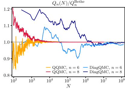
In this paper we show how to apply these integration techniques to perturbative expansions for quantum many-body systems. Our “Quantum Quasi-Monte Carlo” (QQMC) approach is broadly applicable. It can be formulated for both equilibrium and non-equilibrium cases and extended to various lattices and dimensions. Here we demonstrate it on a quantum dot model and show computational accelerations of several orders of magnitude compared to state-of-the-art DiagQMC Profumo et al. (2015); Bertrand et al. (2019a) (Fig. 1). A crucial ingredient of QQMC is the warping of the integral. This is a multi-dimensional change of variables constructed from a model function that approximates the integrand. We show that a simple model already yields remarkable results and propose directions for future optimizations. We demonstrate convergence as fast as $1/N$ in a high-precision benchmark against an exact Bethe Ansatz solution, to order $n=12$. To illustrate the power of QQMC, we calculate the finite-bias current through a quantum dot in the Kondo regime, sweeping electrostatic gating and interaction strength as parameters. This experimentally relevant calculation was computationally unfeasible for previous techniques.

Formalism. In perturbative calculations, an observable $F(U)$ such as a current or susceptibility is expressed as a power series in the interaction $U$:

$$F(U)=\sum_{n=0}^{\infty}F_{n}U^{n},$$ (1)

where the coefficients $F_{n}$ are $n$-dimensional integrals

$$F_{n}=\int\!\textrm{d}^{n}\boldsymbol{u}\,\,f_{n}(u_{1},u_{2},\ldots,u_{n}).$$ (2)

The integrands $f_{n}(\boldsymbol{u})$ are time-ordered correlators expressed in terms of $2^{n}$ determinants (Wick’s theorem), in both Schwinger-Keldysh Profumo et al. (2015) and Matsubara formalisms Rossi (2017). The exponential complexity of evaluating $f_{n}(\boldsymbol{u})$ leads us to seek fast integration methods. Here the $u_{i}$ specify the locations of interaction vertices in space and time. We present the formalism generally and will specialize to a concrete application later.

We will perform the integral Eq. (2) by direct sampling using quasi-Monte Carlo. The crucial step is to warp the integral, i.e. to make a change of variables $\boldsymbol{u}(\boldsymbol{x})$ that maps the hypercube $\boldsymbol{x}\in[0,1]^{n}$ onto the $\boldsymbol{u}$ domain. The integral Eq. (2) becomes

$$F_{n}=\int_{[0,1]^{n}}\!\!\mathrm{d}^{n}\boldsymbol{x}\,\,f_{n}\left[\boldsymbol{u}(\boldsymbol{x})\right]\left|\frac{\partial\boldsymbol{u}}{\partial\boldsymbol{x}}\right|,$$ (3)

where $\left|{\partial\boldsymbol{u}}/{\partial\boldsymbol{x}}\right|$ is the associated Jacobian.

The most important property of the warping is to make the function $\bar{f}_{n}(\boldsymbol{x})=f_{n}\left[\boldsymbol{u}(\boldsymbol{x})\right]\left|{\partial\boldsymbol{u}}/{\partial\boldsymbol{x}}\right|$ as smooth as possible in the new variables $\boldsymbol{x}$. If $f_{n}$ were positive, the perfect change of variables would make $\bar{f}_{n}$ constant and thus trivial to integrate with a single sample. That would be tantamount to ideal sampling from the distribution $f_{n}(\boldsymbol{u})$ and it is as challenging as the original integration. Instead, a judicious warping must provide sufficient smoothing while remaining efficiently computable.

Mathematically, convergence theorems can only be established for $\bar{f}_{n}(\boldsymbol{x})$ that belong to specific smooth function spaces, or whose Fourier coefficients have rapid asymptotic decay properties Dick et al. (2013); Dick and Pillichshammer (2010). Although we cannot prove that our warped integrands satisfy assumptions of this kind, in practice we find that the change of variables are good enough to provide excellent error scaling.

To warp the integral, we consider a positive model function $p_{n}(\boldsymbol{u})$, which should be viewed as an approximation of $|f_{n}|$. The inverse change of variables $\boldsymbol{x}(\boldsymbol{u})$ is then defined by (for $1\leq m\leq n$)

$$x_{m}(u^{\prime}_{m},u_{m+1},\ldots,u_{n})=\dfrac{\int_{0}^{u^{\prime}_{m}}\mathrm{d}u_{m}\int_{0}^{\infty}\prod_{i=1}^{m-1}\mathrm{d}u_{i}\,\,p_{n}(\boldsymbol{u})}{\int_{0}^{\infty}\mathrm{d}u_{m}\int_{0}^{\infty}\prod_{i=1}^{m-1}\mathrm{d}u_{i}\,\,p_{n}(\boldsymbol{u})}$$ (4)

Here we adopt a case where $u_{i}$ is defined on the interval $[0,\infty)$. Since $x_{m}(\boldsymbol{u})$ only depends on $u_{m},\ldots,u_{n}$, the Jacobian is $\left|{\partial\boldsymbol{u}}/{\partial\boldsymbol{x}}\right|=[\int\mathrm{d}\boldsymbol{u}\,\,p_{n}(\boldsymbol{u})]/p_{n}(\boldsymbol{u})$ (see Appendix D). In quasi-Monte Carlo, the integral Eq. (3) is approximated by a sum over the first $N$ points of a low-discrepancy sequence $\boldsymbol{\bar{x}_{i}}$. This is a deterministic sequence of points with specific properties that uniformly samples the hypercube Dick et al. (2013); Dick and Pillichshammer (2010). We have

$$F_{n}\approx F_{n}(N)=\frac{\mathcal{C}}{N}\sum_{i=0}^{N}\dfrac{f_{n}\left[\boldsymbol{u}(\boldsymbol{\bar{x}_{i}})\right]}{p_{n}\left[\boldsymbol{u}(\boldsymbol{\bar{x}_{i}})\right]}$$ (5)

where $\mathcal{C}=\int\mathrm{d}\boldsymbol{u}\,\,p_{n}(\boldsymbol{u})$ is a constant. Here we use a Sobol’ sequence Sobol’ (1967); Kuo and Nuyens (2016) to obtain $\boldsymbol{\bar{x}_{i}}$.

The model function $p_{n}(\boldsymbol{u})$ should have two key properties. First, it should approximate $|f_{n}(\boldsymbol{u})|$ well. Second, its form should be simple enough for the partial integrals Eq. (4) to be evaluated exactly and quickly. This allows the reciprocal function $\boldsymbol{u}(\boldsymbol{x})$ to be computed by first inverting the one-dimensional function $x_{n}(u_{n})$, then inverting $x_{n-1}(u_{n},u_{n-1})$ for fixed $u_{n}$, and so on (see Appendix D).

Many classes of model functions are possible, as discussed later. This paper applies the method to impurity models, using a real-time Schwinger-Keldysh formalism, in which the $u_{i}$ are the times of the interaction vertices. We consider the simple form

$$p_{n}(\boldsymbol{u})=\prod_{i=1}^{n}h^{(i)}\bigl{(}u_{i-1}-u_{i}\bigr{)}.$$ (6)

with $0<u_{n}<u_{n-1}<\ldots<u_{1}<u_{0}$. Here $u_{0}=t$ is defined to be the measurement time and the $h^{(i)}$ are positive scalar functions. (They may depend on $n$, but we omit this index). The factored structure allows Eq. (4) to be inverted rapidly (see Appendix D).

Anderson Impurity. We illustrate our method on the Anderson impurity model coupled to two leads. This is the canonical model for a quantum dot with Coulomb repulsion and the associated Kondo effect. It has been realized in many nanoelectronic experiments Goldhaber-Gordon et al. (1998b, a); Cronenwett et al. (1998); Iftikhar et al. (2018). Importantly, some quantities including the electron occupation on the dot $Q$ can be computed analytically in the universal limit with the Bethe ansatz Tsvelick and Wiegmann (1983); Okiji and Kawakami (1984). This provides us with a high-precision benchmark for QQMC at any perturbation order $n$.

We consider an infinite one-dimensional chain with the impurity at site $i=0$. The non-interacting Hamiltonian is $H_{0}=\sum_{i,\sigma}(\gamma_{i}c^{{\dagger}}_{i,\sigma}c^{{\phantom{\dagger}}}_{i+1,\sigma}+\mathrm{H.c.})+\varepsilon_{d}\sum_{\sigma}c^{{\dagger}}_{0\sigma}c^{{\phantom{\dagger}}}_{0\sigma}$, where $\sigma=\uparrow,\downarrow$ is the electronic spin and $\varepsilon_{d}$ represents a capacitive gate coupled to the dot. The local Coulomb repulsion is $H_{\mathrm{int}}=Uc^{{\dagger}}_{0\uparrow}c^{{\phantom{\dagger}}}_{0\uparrow}c^{{\dagger}}_{0\downarrow}c^{{\phantom{\dagger}}}_{0\downarrow}$. The electron tunneling between the leads and dot is $\gamma_{0}=\gamma_{-1}=\gamma$. All other $\gamma_{i}=D/2$, corresponding to hopping within the leads; the lead half-bandwidth $D$ is a constant. We perform the perturbative expansion in powers of $U$ (see Appendix E).

Benchmark. To validate the QQMC method, we consider the special case solved by the Bethe Ansatz. For this, we set temperature $T=0$, capacitive gate $\varepsilon_{d}=0$, and half-bandwidth $D\rightarrow+\infty$ such that $\Gamma=4\gamma^{2}/D=1$ is the unit of energy. The measurement time $t=30/\Gamma$ is sufficiently long that the system reaches steady-state. We compute the expansion of the occupation number $Q(U)=\langle c^{{\dagger}}_{0\uparrow}c^{{\phantom{\dagger}}}_{0\uparrow}+c^{{\dagger}}_{0\downarrow}c^{{\phantom{\dagger}}}_{0\downarrow}\rangle$. The system is particle-hole symmetric for $\varepsilon_{d}=-U/2$ so the non-interacting case is $Q_{0}=1$. For higher-order $Q_{n}$, particle-hole symmetry is broken, but the expansion stays in the symmetric regime $(U+2\varepsilon_{d})\ll\sqrt{U\Gamma}$ Tsvelick and Wiegmann (1983).

Figure 2 shows the relative error between $Q_{n}(N)$ using QQMC and the exact result $Q^{\mathrm{Bethe}}_{n}$ (see Appendix F), as a function of the number of integrand evaluations $N$. Following an initial transient, we enter an asymptotic regime in which there is rapid convergence: for $n=4$ this is consistent with pure $1/N$ while for $n=8,12$ it is $1/N^{\delta}$ with $\delta\simeq 0.9,0.8$. These calculations used the product model function Eq. (6) with a single exponential $h^{(i)}(v_{i})=\exp(-v_{i}/\tau)$, where $\tau=0.95$. The same set-up was used in Fig. 1. The level of precision that we obtained revealed limitations in the conventional evaluation of the non-interacting Green functions, which warranted special consideration (see Appendix E).

\begin{overpic}[scale={1}]{fig2_Qn_convergence_orders.pdf} \put(10.0,10.0){\includegraphics[scale={0.4}]{imp_cartoon.pdf}} \end{overpic}

Figure 2: Expansion coefficients $Q_{n}$ for the Anderson impurity occupation number relative to the analytic result $Q^{\mathrm{Bethe}}_{n}$. QQMC converges at rates close to $1/N$ with the number of integrand evaluations $N$. For visibility, the data has been smoothed (see Appendix H). The black lines indicate exact $1/N$ (dotted) and $1/\sqrt{N}$ (dashed) convergence. Each run was performed with one Sobol’ sequence. Inset: Cartoon of quantum dot set-up.

It is expected that the convergence rate gradually slows as $n$ increases. First, the quality of the warping decreases as the disparity between the increasingly-severe requirements of convergence theory and the behavior of our integrands grows. This can be mitigated by constructing more expressive model functions, which we discuss below. Second, for larger $n$ the integrands generally become more oscillatory. The model functions Eq. (4) were not designed to handle cases with massive cancellation, and this may become a limiting factor. We will see this effect below for calculations with $\varepsilon_{d}/U>0.5$, although in practice enough orders can be computed accurately to obtain the desired physical results (see Appendix E).

In Quasi-Monte Carlo methods, a standard technique to estimate errors is to perform computations using Eq. (5) with several ‘randomized’ low-discrepancy sequences Dick et al. (2013); Nuyens ; Dick and Pillichshammer (2010); L’Ecuyer (2018) and we use this method below (see Appendix G).

Having made these technical points, let us reiterate the lessons of Fig. 1 and Fig. 2: (i) QQMC provides a dramatic speed-up with better asymptotic error scaling than DiagQMC; (ii) the speed-up persists up to at least order $n=12$, which is what is needed for practical applications.

Coulomb Diamond. We now apply QQMC to solve a topical physics problem. We explore the current-voltage characteristic $I(V)$ across the quantum dot for finite bias and varying $U$. Since quantum dots are considered promising platforms for building qubit systems, it is of primary importance to understand how many-body effects influence their properties, especially the phase coherence.

Quantum dots can be in three different experimentally accessible regimes Tans et al. (1997); Nygård et al. (2000); Liang et al. (2001); Roch et al. (2008): Fabry-Pérot (small $U$), Kondo (intermediate $U$) and Coulomb blockade (large $U$). The Fabry-Pérot and Coulomb blockade limits are well described by, respectively, non-interacting and semi-classical theories; the out-of-equilibrium Kondo regime is more challenging. Two controlled approaches have recently appeared, but both are too slow for some applications: the Schwinger-Keldysh DiagQMC used in Figs. 1 and 4 Profumo et al. (2015); Bertrand et al. (2019a) and the real-time inchworm algorithm Cohen et al. (2015); Ridley et al. (2019); Krivenko et al. (2019). QQMC provides the speed and precision to allow large parameter sweeps, which is mandatory to make good contact with experiments. In Bertrand et al. (2019a), some of us studied the Kondo ridge close to $\varepsilon_{d}=-U/2$. QQMC allows us to present results scanning the entire $(U,\varepsilon_{d})$ phase diagram, including slowly converging regions with even numbers of electrons or near the degeneracy points.

Figure 3: Current at finite bias voltage through the Anderson impurity at $T=0$, sweeping through several interaction regimes. Each point is a different QQMC calculation up to order $n=10$, including series resummation Bertrand et al. (2019a). The error bars are a combination of integration error and truncation error of the resummation; the latter dominates. By construction, the data is symmetric with respect to the particle-hole symmetric point $\varepsilon_{d}=-U/2$. Inset: Coulomb diamond in the Coulomb blockade picture (large $U$). Regions where current can flow are shaded grey. The dashed line indicates the scan shown in the main plot (varying $\varepsilon_{d}$ for fixed $V/U=1/7$).

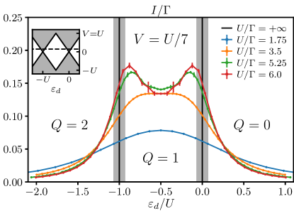
Figure 3 (inset) shows a cartoon of the differential conductance for varying $(\varepsilon_{d},V)$ as predicted by Coulomb blockade theory Beenakker (1991) and seen experimentally at low temperatures and large $U$ Hofheinz et al. (2007). At small bias, the Coulomb blockade forbids current flows except at two special points: $\varepsilon_{d}=0$, where the dot energies for $Q=0$ and $Q=1$ electrons are degenerate, and $\varepsilon_{d}=-U$ (likewise for $Q=1,2$). At intermediate $U$, the Kondo effect changes this picture drastically: the zero-bias Kondo resonance forms in the ‘forbidden’ region of odd $Q$ and enables current flow.

Figure 3 shows the current $I$ versus gate voltage $\varepsilon_{d}$ for $V=U/7$ and temperature $T=0$. We choose a finite half-bandwidth $D/\Gamma=20$ (see Appendix E). Sweeping the interaction $U/\Gamma$ shows several regimes. For $U/\Gamma=1.75,3.5$ a current plateau emerges in the local moment regime ($Q=1$) due to Kondo resonance formation. The current develops new local maxima seen for $U/\Gamma=5.25,6.00$. These grow toward the Coulomb blockade limit at larger $U$ (black lines); at the same time, current around $\varepsilon_{d}/U=-0.5$ reaches a maximum and decreases. This is a competition between resonance formation and narrowing. At small $U$, the Kondo temperature $T_{K}$ is much larger than the bias $V$ and we are in the linear response regime. In this regime near $\varepsilon_{d}=-U/2$ we approach perfect transmission $I=V/\pi$; see Ref. Bertrand et al. (2019a). At larger $U\gtrsim 4\Gamma$, $T_{K}$ decreases exponentially with $U$ and become smaller than $V$, leaving the linear response regime. Throughout, as $U$ increases, the already-small current in the side regions ($Q=0,2$) is increasingly suppressed.

Figure 4: Comparison of convergence of $Q_{8}$ for different methods of integration: evaluating unwarped integrand with a Sobol’ sequence (cyan), DiagQMC (red), warped integral sampled with Mersenne Twister pseudo-random numbers (green) or Sobol’ sequence (blue). For the warped cases, we used Eq. (6) with $h^{(i)}(v_{i})=\exp(-v_{i}/\tau),\tau=0.95$. After an initial warping with exponential functions $\tau=1.1$, we can apply an additional warping obtained by projection (orange); see Appendix I. For visibility, data (except Sobol’ and DiagQMC) has been smoothed in the same way as in Fig. 2.

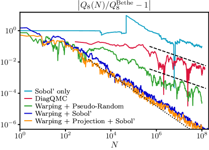
Model Function. Let us reexamine the importance of integral warping and model functions. Figure 4 shows the convergence of $Q_{8}(N)$ using different integration methods; parameters are identical to Fig. 2. When the integral is evaluated using Sobol’ points without warping (‘Sobol’ only’) the convergence is poor, showing that naively applying low-discrepancy sequences provides little benefit for these integrands. Next, contrast regular DiagQMC with the warped integrand using pseudo-random numbers. As expected for pure Monte Carlo approaches, both show $1/\sqrt{N}$ convergence. Nonetheless, sampling the warped integrand still converges faster than DiagQMC, despite the fact that the latter uses importance sampling via the Metropolis algorithm. As anticipated, QQMC using Sobol’ points and the model function Eq. (6) based on exponential $h^{(i)}$ converges even more rapidly.

How can the model function Eq. (6) with simple $h^{(i)}$ provide such dramatic convergence improvements? Our integrands describe physical correlators that are highly structured and have decaying exponential or power-law tails; see Appendix I and Refs. Profumo et al. (2015); Bertrand et al. (2019b). The tail contributions become ever more important as the dimension increases. The model function properly describes the long-time asymptotics (see Appendix I). We also emphasize the importance of a well-chosen coordinate system in the model function: the differences of closest times $v_{i}=u_{i-1}-u_{i}$ used to parametrize the $h^{(i)}$.

Optimization of the model function should allow further performance gains, particularly at higher orders $n$. One possibility is to better adapt the functions $h^{(i)}$ to $f_{n}$. To illustrate this, we apply a second warping constructed by sampling points from the first warping. These samples are projected along the dimensions of $v$ space and smoothed; see Appendix I for details. As shown in Fig. 4, this optimization reduces the error by a factor of $\simeq 2$. More importantly, it automatically gives robust convergence without the need to manually optimize the $\tau$ parameter.

Finally, other families of model functions exist beyond Eq. (6), that provide versatile and expressive approximations while still allowing for fast inversion of Eq. (4). One such family is Matrix Product States (MPS) or functional tensor-trains Schollwöck (2011); Glasser et al. , of which Eq. (6) is just the simplest case:

$$p_{n}(\boldsymbol{u})=h^{(1)}_{a}(v_{1})h^{(2)}_{ab}(v_{2})\cdots h^{(n-1)}_{cd}(v_{n-1})h^{(n)}_{d}(v_{n}).$$ (7)

Here $h^{(i)}_{ab}$ are matrices and repeated indices are summed. Another promising family is $p_{n}(\boldsymbol{u})=\prod_{i=1}^{n-1}\bar{h}^{(i)}(v_{i+1},v_{i}).$

Conclusion. We have shown how to use sampling techniques based on low-discrepancy sequences to compute high orders of many-body perturbation theory. Although we cannot show that the integrands obey the assumptions of formal Quasi-Monte Carlo convergence theory, practical scaling as fast as $1/N$ is still achievable. This success was possible due to the warping of the integral based on a model function. Using benchmarks on exactly solvable quantities in the Anderson impurity model, we unambiguously validated the convergence of this ‘Quantum Quasi-Monte Carlo’ (QQMC) method at high-precision. This calculation was about $\sim 10^{4}$ times faster than the DiagQMC equivalent.

We can apply the techniques established here to models with interesting strongly correlated physics in all dimensions, for equilibrium and especially non-equilibrium situations. For continuum models, the integrands are smooth and warping should be particularly simple. For lattice models, the discrete summation may degrade convergence, although this may be addressed with sufficiently good model functions. QQMC can also be applied to other diagrammatic expansions, e.g. in hybridization Cohen et al. (2015). Constructing more expressive model functions should further increase speed and accuracy and is an ideal application for recent machine learning techniques in quantum systems.

Finally, we have shown in our calculations that the simple model function Eq. (6) captures the behavior of perturbation theory integrands in asymptotic large-coordinate regions. This is not accidental, but reveals a simplifying structure of the correlation functions arising from Wick’s theorem that was not previously appreciated in diagrammatic numerical simulations. For the real-time Schwinger-Keldysh calculations, the contour index means that the MPS structure Eq. (7) is the natural approximation for generic many-body systems. It can be used as a starting point to efficiently compute and integrate these functions, even beyond the Monte Carlo or QQMC sampling discussed here.

Appendix A Low-Discrepancy Sequences

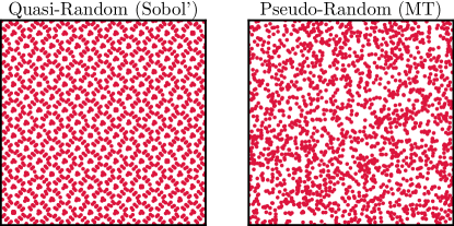
The integration technique for perturbation theory integrals we presented in the main manuscript is based on so-called ‘quasi-Monte Carlo’ methods, which use sampling with low-discrepancy sequences. Despite the naming, such quasi-random sequences are highly structured and deterministic, unlike the pseudo-random number sequences used in conventional Monte Carlo sampling (see Fig. 5). Here we briefly summarize the history of this field of mathematics as well as key features of these sequences.

Figure 5: Sampling the two-dimensional square $[0,1]^{2}$ with quasi-random numbers from a Sobol’ sequence (left) and pseudo-random numbers from a Mersenne-Twister sequence (right). The Sobol’ sequence gives a far more uniform sampling.

The roots of low-discrepancy and quasi-random sequences lie in the ancient field of Diophantine Approximation – the theory of approximating sets of real numbers by rational ones, especially in its modern form pioneered by Roth Roth (1954) – and in Weyl’s early efforts to characterize uniformity of distributions Weyl (1916). These methods were applied to practical multidimensional integration in the late 1950’s and 1960’s, with contributions from, among many others, Korobov Korobov (1957) and Sobol’ Sobol’ (1967) in the USSR and Hammersley Hammersley (1960) (building on work by van der Corput van der Corput (1935)), Halton Halton (1960) and Haselgrove Haselgrove (1961) in the UK. There was even an unsuccessful attempt to use them as a component of Markov Chain Monte Carlo simulation for multi-point physical integrals in 1951 Richtmyer (1952). Niederreiter Niederreiter (1978) surveys much of the early work in this area. Since that time, quasi-Monte Carlo methods have become standard in many fields including, for example, computational chemistry Conroy (1967). Indeed, convergence rate improvements analogous to, but smaller than, ours are seen in molecular excitation computations Berblinger and Schlier (1991). Most of the early applications had relatively low dimensions $\lesssim 10$. However, the field was rejuvenated in the late 1990’s and early 2000’s by the discovery that quasi-Monte Carlo works unexpectedly well for certain high-dimensional financial integrals stemming from discretized stochastic partial differential equations Paskov and Traub (1995). This was followed by the application of Reproducing Kernel Hilbert Space theory to explain this success (see e.g. Ref. Wang and Sloan (2005)), and the advent of ‘fast component-by-component’ construction techniques to create optimized quasi-random generators for these problems Nuyens and Cools (2006). A survey of this more recent work appears in Ref. Dick et al. (2013).

The main strength of quasi-Monte Carlo relative to Markov Chain Monte Carlo is its greatly accelerated convergence rate in applications with well-behaved integrands. Its main disadvantage is its reduced flexibility. Quasi-Monte Carlo methods require highly symmetric integration domains – usually hypercubes – and careful preparation of the integrand. In our approach we implement this through a change of coordinates and warping. However, perhaps most importantly, they are intrinsically non-adaptive during a calculation: changing the distribution during the main sampling run destroys its carefully constructed uniformity properties, which typically reduces the convergence rate to Monte Carlo scaling $O(1/\sqrt{N})$. To handle generic integrands whose properties are unknown in advance, separate runs and analysis are needed before the main sampling run.

Finally, we note that the theory of quasi-Monte Carlo typically gives worst-case error bounds, but not average-case ones. This is because no stochastic averaging is done. An exception is when we perform averaging of random shifts. These worst-case bound are theoretically tight but often rather pessimistic compared to observed behavior. For pure Monte Carlo methods, the opposite situation is true and we typically have average-case but not worst-case bounds.

Appendix B Summary of the QQMC algorithm

Below, we summarize the QQMC algorithm. More details on the building blocks are given in other sections of this supplementary material. Note that unlike usual diagrammatic Monte Carlo techniques, the coefficients $F_{n}$ for different orders $n$ are calculated separately.

Preprocessing steps.

• Calculate non-interacting Green functions in real time. These functions form the basic elements from which the integrands are calculated. They can be obtained through Fourier transform of the real frequency Green functions which can be obtained analytically or numerically.

• Calculate Warping. Once a model function $p_{n}(\boldsymbol{u})$ has been selected and possibly adapted to the integrand (see projection method below), construct the mapping $\boldsymbol{x}(\boldsymbol{u})$ by computing the partial cumulative functions of the model function $p_{n}(\boldsymbol{u})$.

• For each component of the mapping $\boldsymbol{x}(\boldsymbol{u})$, invert it to obtain the inverse mapping $\boldsymbol{u}(\boldsymbol{x})$. This can be done, for example, be interpolating the original mapping $\boldsymbol{x}(\boldsymbol{u})$ on a sufficiently fine linear mesh and inverting.

• Initialize $r=0$.

Main computing loop. For each sample point $i\in 1\dots N$,

• Generate the low-discrepancy quasi-random vector $\boldsymbol{x}_{i}$. These vectors span uniformly the hypercube $[0,1]^{n}$.

• Calculate the corresponding point $\boldsymbol{u}_{i}=\boldsymbol{u}(\boldsymbol{x}_{i})$ in the original integration space.

• Calculate the corresponding value of the integrand $f^{(i)}=f_{n}(\boldsymbol{u}_{i})$ and the value of the model function $p^{(i)}=p_{n}(\boldsymbol{u}_{i})$.

• Update the result $r\rightarrow r+f^{(i)}/p^{(i)}$

Returns. The final estimate of the observable is $F_{n}\approx r/N$.

Appendix C Benchmarking at higher orders

Figure 6: Relative error (upper) an absolute error (lower) of $Q_{n}$ versus perturbation theory order $n$ for our benchmark calculation against Bethe ansatz results, up to $n=22$. Different curves correspond to different numbers of calculated points $N$. We used Eq. (6) with $h^{(i)}(v_{i})=\exp(-v_{i}/\tau)$ with $\tau=0.95$ for $n\leq 15$ and $\tau=0.90$ for $n\geq 16$. The parameters are the same as in Fig. 1.

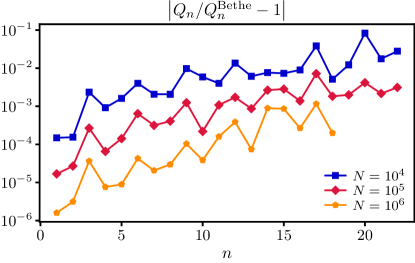
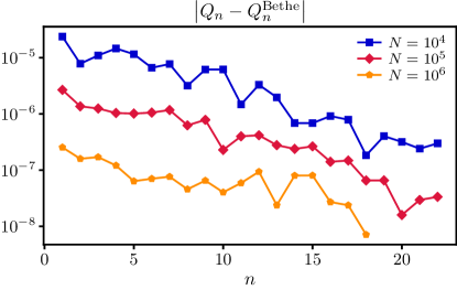
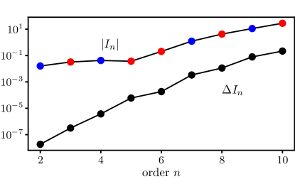
The main manuscript focuses on data for perturbation theory orders $n\lesssim 12$, where QQMC enables calculations with an unprecedented precision of up to six or seven digits. In this section, we show additional data for a smaller number of samples $N$. This enables us to calculate much larger orders up to $n=22$, well beyond previous diagrammatic quantum Monte Carlo techniques. We recall that the a single evaluation of the integrand $f_{n}(\boldsymbol{u})$ has an exponential complexity $\sim 2^{n}$, which has limited previous calculations to order $n\leq 15$ with less than two digits precisions. While $N=10^{5}$ is not yet deep into the asymptotic regime, we find that we could reach two to three digits of accuracy.

The data are presented in Fig. 6 respectively for the relative error (top panel) and absolute error (lower panel). Although the error deteriorates with the order $n$, the speed up provided by QQMC more than compensates for the imperfection of the model function. We find that the absolute error actually decreases with $n$ as the $Q_{n}$ gets smaller at large $n$.

Appendix D Model Function Properties

Here we expand on the properties of the change of variables $\boldsymbol{x}(\boldsymbol{u})$ arising from the model $p_{n}(\boldsymbol{u})$. These were defined in the main text as:

$$x_{m}(u^{\prime}_{m},\ldots,u_{n})=\dfrac{\int_{0}^{u^{\prime}_{m}}\mathrm{d}u_{m}\int_{0}^{\infty}\prod_{i=1}^{m-1}\mathrm{d}u_{i}\,\,p_{n}(\boldsymbol{u})}{\int_{0}^{\infty}\mathrm{d}u_{m}\int_{0}^{\infty}\prod_{i=1}^{m-1}\mathrm{d}u_{i}\,\,p_{n}(\boldsymbol{u})}$$ (4^′)

To understand the structure of Eq. (4^′) and how it can be useful when sampling from $p_{n}(\boldsymbol{u})$, let us consider the explicit transformation for small orders $n$.

For $n=1$, Eq. (4^′) is simply the normalized cumulative function $x_{1}(u_{1})=\int_{0}^{u_{1}}\mathrm{d}\bar{u}_{1}p_{1}(\bar{u}_{1})/\int_{0}^{\infty}\mathrm{d}\bar{u}_{1}p_{1}(\bar{u}_{1})$ which upon differentiation gives,

$$dx_{1}=\frac{p_{1}(u_{1})\mathrm{d}u_{1}}{\int_{0}^{\infty}\mathrm{d}\bar{u}_{1}\,\,p_{1}(\bar{u}_{1})}.$$ (8)

This means that uniformly sampling $x_{1}$ leads to the sampling of $p(u_{1})$. In practice, one need to invert the cumulative distribution $x_{1}(u_{1})$ which can be done through interpolation techniques.

Next, let us consider the procedure for $n=3$ using a model function $p_{3}(u_{1},u_{2},u_{3})$. The reverse coordinate transform $\boldsymbol{x}(\boldsymbol{u})$ is

$$x_{1}(u_{1},u_{2},u_{3}) =\frac{\int_{0}^{u_{1}}\mathrm{d}\bar{u}_{1}\,\,p_{3}(\bar{u}_{1},u_{2},u_{3})}{\int_{0}^{\infty}\mathrm{d}\bar{u}_{1}\,\,p_{3}(\bar{u}_{1},u_{2},u_{3})}$$

$$x_{2}(u_{2},u_{3}) =\frac{\int_{0}^{u_{2}}\mathrm{d}\bar{u}_{2}\,\,\int_{0}^{\infty}\mathrm{d}\bar{u}_{1}\,\,p_{3}(\bar{u}_{1},\bar{u}_{2},u_{3})}{\int_{0}^{\infty}\mathrm{d}\bar{u}_{2}\,\,\int_{0}^{\infty}\mathrm{d}\bar{u}_{1}\,\,p_{3}(\bar{u}_{1},\bar{u}_{2},u_{3})}$$ (9)

$$x_{3}(u_{3}) =\frac{\int_{0}^{u_{3}}\mathrm{d}\bar{u}_{3}\int_{0}^{\infty}\mathrm{d}\bar{u}_{2}\int_{0}^{\infty}\mathrm{d}\bar{u}_{1}\,\,p_{3}(\bar{u}_{1},\bar{u}_{2},\bar{u}_{3})}{\int_{0}^{\infty}\mathrm{d}\bar{u}_{3}\int_{0}^{\infty}\mathrm{d}\bar{u}_{2}\int_{0}^{\infty}\mathrm{d}\bar{u}_{1}\,\,p_{3}(\bar{u}_{1},\bar{u}_{2},\bar{u}_{3})}$$

The consecutive coordinate integration, gives the coordinate transformation a special structure: $x_{3}(u_{3})$ does not depend on $u_{1},u_{2}$ and $x_{2}(u_{3},u_{2})$ does not depend on $u_{1}$. This means that the Jacobian matrix for the reverse coordinate transformation $\boldsymbol{x}(\boldsymbol{u})$ has an upper-triangular form

$$\left[\frac{\partial\boldsymbol{x}}{\partial\boldsymbol{u}}\right]=\left[\begin{array}[]{ccc}({\partial x_{1}}/{\partial u_{1}})&({\partial x_{1}}/{\partial u_{2}})&({\partial x_{1}}/{\partial u_{3}})\\ 0&({\partial x_{2}}/{\partial u_{2}})&({\partial x_{2}}/{\partial u_{3}})\\ 0&0&({\partial x_{3}}/{\partial u_{3}})\end{array}\right]$$ (10)

so that the Jacobian determinant is simply

$$\left|\frac{\partial\boldsymbol{x}}{\partial\boldsymbol{u}}\right|=\frac{\partial x_{1}}{\partial u_{1}}\cdot\frac{\partial x_{2}}{\partial u_{2}}\cdot\frac{\partial x_{3}}{\partial u_{3}}.$$ (11)

Differentiating Eq. (9), cancelling common factors and using $\left|{\partial\boldsymbol{u}}/{\partial\boldsymbol{x}}\right|=1/\left|{\partial\boldsymbol{x}}/{\partial\boldsymbol{u}}\right|$ gives

$$\left|\frac{\partial\boldsymbol{u}}{\partial\boldsymbol{x}}\right|= \frac{\int_{0}^{\infty}\mathrm{d}u_{3}\int_{0}^{\infty}\mathrm{d}u_{2}\int_{0}^{\infty}\mathrm{d}u_{1}\,\,p_{3}(u_{1},u_{2},u_{3})}{p_{3}(u_{1},u_{2},u_{3})}.$$ (12)

The same procedure straightforwardly generalizes to an arbitrary number of dimensions $n$. This reproduces the result quoted in main text:

$$\left|\frac{\partial\boldsymbol{u}}{\partial\boldsymbol{x}}\right|=\frac{\int_{0}^{\infty}\prod_{i=1}^{n}\mathrm{d}u_{i}\,\,p_{n}(\boldsymbol{u})}{p_{n}(\boldsymbol{u})}.$$ (13)

In practice, we uniformly sample the hypercube $[0,1]^{3}$ using Sobol’ sequence to obtain $(x_{1},x_{2},x_{3})$. From $x_{3}$ one obtains $u_{3}$ by inverting the one dimensional equation $x_{3}(u_{3})$. With the obtained value of $u_{3}$, the equation $x_{2}(u_{2},u_{3})$ becomes a one dimensional function of $u_{2}$ which can be inverted. Last with the obtained $(u_{2},u_{3})$, one can invert $x_{1}(u_{1},u_{2},u_{3})$ to obtain $u_{1}$.

Product Model. While the coordinate transform described above is very general, it is only useful if the multiple integrals in Eq. (4^′) can be performed efficiently. Otherwise, it is as or more costly than the actual integral of the perturbation series coefficient that we wish to compute.

The product model function

$$p_{n}(\boldsymbol{u})=\prod_{i=1}^{n}h^{(i)}\bigl{(}u_{i-1}-u_{i}\bigr{)},$$ (6^′)

is particularly efficient. It is simpler to view this as a composition of two transforms. First, we change variables $v_{i}=u_{i-1}-u_{i}$, which has Jacobian $\left|{\partial\boldsymbol{u}}/{\partial\boldsymbol{v}}\right|=1$. Second, in the $v_{i}$ variables, the coordinate transform Eq. (4^′) separates entirely, so that each $x_{m}$ only depends on a single variable $v_{m}$:

$$x_{m}(v_{m})=\frac{\int_{0}^{v_{m}}\mathrm{d}\bar{v}_{m}\,\,h^{(m)}(\bar{v}_{m})}{\int_{0}^{\infty}\mathrm{d}\bar{v}_{m}\,\,h^{(m)}(\bar{v}_{m})}$$ (14)

These one-dimensional integrals can be integrated quickly and precisely analytically or using quadrature algorithms. We then invert $x_{m}(v_{m})$ numerically to find the coordinate transform $v_{m}(x_{m})$. In practice, it is possible to completely pre-compute these integrals on a fine mesh for fast evaluation during calculation.

We note that the product form Eq. (6^′) is known for importance sampling in Monte Carlo applications, e.g. as part of the VEGAS algorithm Lepage (1978, 1980). The choice of coordinate system $v_{i}$ as compared to $u_{i}$ affects the quality of model function and is an important physical consideration.

MPS Model. The model function Eq. (7) can also be efficiently computed using the above algorithm and standard MPS techniques Schollwöck (2011). Unlike the product model, the integrations for different $v_{i}$ have to be performed in sequence, with a matrix-vector multiplication at each step.

Appendix E Explicit expressions of the integrands

In this appendix, we will describe the Anderson impurity model as well as the perturbation expansion formalism of our calculations in more detail.

E.1 Model

The Hamiltonian of the Anderson impurity model is $H=H_{0}+H_{\rm int}\theta(t)$, with the non-interacting term:

$$H_{0}=\sum_{i,\sigma}\left(\gamma_{i}c^{\dagger}_{i,\sigma}c^{\phantom{\dagger}}_{i+1,\sigma}+H.c.\right)+E_{d}\sum_{\sigma}c^{\dagger}_{0\sigma}c^{\phantom{\dagger}}_{0\sigma}.$$ (15)

The hopping parameters are all $\gamma_{i}=D/2$, except at the impurity ($i=0$) where $\gamma_{0}=\gamma_{-1}=\gamma$. The interaction term is

$$H_{\rm int}=U(c^{\dagger}_{0\uparrow}c^{\phantom{\dagger}}_{0\uparrow}-\alpha)(c^{\dagger}_{0\downarrow}c^{\phantom{\dagger}}_{0\downarrow}-\alpha),$$ (16)

where $\alpha$ is a quadratic shift to the perturbation. This shift means that the $U$ expansion is performed about a different starting point, and is commonly used to improve perturbation series convergence Profumo et al. (2015); Rubtsov and Lichtenstein (2004); Wu et al. (2017). Note that the energy of a single electron localized on the impurity is $\varepsilon_{d}=E_{d}-\alpha U$. A symmetric voltage bias $V$ is applied between the two leads. As is standard in the Keldysh formalism, $H_{\mathrm{int}}$ is turned on at time $t=0$ and observables are computed after a large time $t$ when the stationary regime has been reached.

By integrating out the leads, their effect on the dot is represented by a retarded hybridization function $\Delta(\omega)$. The non-interacting dot retarded Green function is $g^{R}(\omega)\equiv 1/(\omega-E_{d}-\Delta(\omega))$. By symmetry, all Green functions are the same for spin up and down.

The density of states of the leads is semi-circular with half-bandwidth $D$. An important parameter of the non-interacting model is the tunneling rate from the impurity to the leads at the (equilibrium) Fermi level $\Gamma=4\gamma^{2}/D$. In terms of $D$ and $\Gamma$, the hybridization function is

$$\Delta(\omega)=\frac{\Gamma}{D}\times\begin{cases}\left(\omega+\sqrt{\omega^{2}-D^{2}}\right)&\text{for $\omega<-D$}\\ \left(\omega-i\sqrt{D^{2}-\omega^{2}}\right)&\text{for $-D<\omega<D$}\\ \left(\omega-\sqrt{\omega^{2}-D^{2}}\right)&\text{for $\omega>D$}\end{cases}$$ (17)

The Bethe ansatz provides results only in the universal regime, where $D\rightarrow+\infty$ with $\Gamma$ fixed. In this limit, the density of states becomes independent of energy (flat band). The hybridization function is simply $\Delta(\omega)=-i\Gamma$. When comparing results to the Bethe ansatz, we we will always work in this regime.

E.2 Expressions for the integrands of series expansions

To obtain the number of electrons $Q$ or the current $I$, we compute a perturbation series in $U$ for the equal-time lesser Green function $G^{<}_{0i}(t,t)=-i\langle c^{\dagger}_{0\uparrow}(t)c^{\phantom{\dagger}}_{i\uparrow}(t)\rangle$, where the creation and annihilation operators are in the Heisenberg picture. We take $i=0$ (on-site) to obtain $Q$, and $i=1$ (dot-lead) to obtain $I$ Meir and Wingreen (1992).

For $\alpha=0$, this series can be written compactly using the “Wick determinant” notation introduced in Ref. Bertrand et al. (2019b):

$$G^{<}_{0i}(t,t)=\sum_{n\geq 0}\frac{i^{n}U^{n}}{n!}\int_{0}^{t}\prod_{k=1}^{n}du_{k}\\ \times\sum_{a_{1},\ldots,a_{n}}(-1)^{\sum a_{k}}\left\llbracket\begin{matrix}(0,t,0),U_{1},\ldots,U_{n}\\ (i,t,1),U_{1},\ldots,U_{n}\end{matrix}\right\rrbracket\left\llbracket\begin{matrix}U_{1},\ldots,U_{n}\\ U_{1},\ldots,U_{n}\end{matrix}\right\rrbracket,$$ (18)

where $a_{k}\in\{0,1\}$ are Keldysh indices, and $U_{k}=(0,u_{k},a_{k})$ represents a point on the Keldysh contour composed of a site index (here $0$ for the impurity), a time $u_{k}$ and a Keldysh index $a_{k}$. The Wick determinant $\left\llbracket\begin{matrix}\ldots\\ \end{matrix}\right\rrbracket$ is defined, for $A_{1},\ldots,A_{m}$ and $B_{1},\ldots,B_{m}$ any set of points on the Keldysh contour, in the case $\alpha=0$, the Wick determinant

$$\left\llbracket\begin{matrix}A_{1},\ldots,A_{m}\\ B_{1},\ldots,B_{m}\end{matrix}\right\rrbracket=\begin{vmatrix}{g}(A_{1},B_{1})&\ldots&{g}(A_{1},B_{m})\\ \vdots&\ddots&\vdots\\ {g}(A_{m},B_{1})&\ldots&{g}(A_{m},B_{m})\end{vmatrix},$$ (19)

where

$$g[(x,u,a),(x^{\prime},u^{\prime},a^{\prime})]=\begin{pmatrix}g^{T}_{xx^{\prime}}(t,t^{\prime})&g^{<}_{xx^{\prime}}(t,t^{\prime})\\ g^{>}_{xx^{\prime}}(t,t^{\prime})&g^{\bar{T}}_{xx^{\prime}}(t,t^{\prime})\end{pmatrix}_{aa^{\prime}},$$ (20)

is the non-interacting one-particle Keldysh Green function. Here $g^{T}$, $g^{\bar{T}}$, $g^{<}$ and $g^{>}$ are respectively the time-ordered, anti-time-ordered, lesser and greater Green functions. In Eq. (18), the determinant on the left is from spin up operators, while the one on the right is from spin down operators. Nevertheless, by spin symmetry their elements share the same Green functions $g$.

The case $\alpha\neq 0$ is similar, but the diagonal terms of the Wick determinants in Eq. (18) must be shifted by $-i\alpha$, except the one connecting to the measurement point (involving the Green function at time $t$) Profumo et al. (2015).

Provided that the non-interacting Green function $g$ is known as a function of time, Eq. (18) explicitly defines the integrand that we refer to in the main text of this article. We compute the time domain Green functions by Fourier transform of the Green functions $g^{<}(\omega)$ and $g^{>}(\omega)$. These can be derived in the Schwinger–Keldysh formalism Meir and Wingreen (1992):

$$g_{00}^{<}(\omega)= 2i|g^{R}(\omega)|^{2}\textrm{Im}[\Delta(\omega)]$$ (21)

$$\times\left[n_{\rm F}\left(\omega-\frac{V}{2}\right)+n_{\rm F}\left(\omega+\frac{V}{2}\right)\right]$$

$$g_{00}^{>}(\omega)= g_{00}^{<}(\omega)-4i|g^{R}(\omega)|^{2}\textrm{Im}[\Delta(\omega)]$$ (22)

$$\gamma g_{01}^{<}(\omega)= \frac{\Delta(\omega)}{2}g^{<}_{00}(\omega)-2i\;n_{\rm F}\!\left(\omega+\frac{V}{2}\right)\textrm{Im}[\Delta(\omega)]g^{R}(\omega)^{*}$$ (23)

Here $n_{\mathrm{F}}(\omega)$ is the Fermi function. Note that the function $g_{0i}^{>}$ is not used in Eq. (18).

$n$	Occupation Number $Q^{\mathrm{Bethe}}_{n}$
$0$	$1$	$\phantom{-}1.000000000000000000000000$
$1$	$-\frac{1}{\pi}$	$-0.3183098861837906715377675$
$2$	$\frac{1}{\pi^{2}}$	$\phantom{-}0.1013211836423377714438795$
$3$	$\frac{\pi^{2}-9}{3\pi^{3}}$	$\phantom{-}0.009348692094998422959323018$
$4$	$\frac{90-11\pi^{2}}{6\pi^{4}}$	$-0.03176576952402088647648727$
$5$	$-\frac{9450-1175\pi^{2}+18\pi^{4}}{90\pi^{5}}$	$\phantom{-}0.01428453978718527764087931$
$6$	$\frac{945}{\pi^{6}}-\frac{3185}{27\pi^{4}}+\frac{137}{60\pi^{2}}$	$\phantom{-}0.003296943760155087659102276$
$7$	$-\frac{10395}{\pi^{7}}+\frac{11690}{9\pi^{5}}-\frac{2653}{100\pi^{3}}+\frac{1}{7\pi}$	$-0.007417285598070720865765088$
$8$	$\frac{135135}{\pi^{8}}-\frac{912065}{54\pi^{6}}+\frac{524881}{1500\pi^{4}}-\frac{363}{140\pi^{2}}$	$\phantom{-}0.003074980697930490893903131$
$9$	$-\frac{2027025}{\pi^{9}}+\frac{41046005}{162\pi^{7}}-\frac{118576073}{22500\pi^{5}}+\frac{623873}{14700\pi^{3}}-\frac{1}{9\pi}$	$\phantom{-}0.001257173321207511996877863$
$10$	$\frac{34459425}{\pi^{10}}-\frac{348898550}{81\pi^{8}}+\frac{5045327287}{56250\pi^{6}}-\frac{761337511}{1029000\pi^{4}}+\frac{7129}{2520\pi^{2}}$	$-0.002096420663210080104411625$
$11$	$-\frac{654729075}{\pi^{11}}+\frac{19887342475}{243\pi^{9}}-\frac{287681226833}{168750\pi^{7}}+\frac{306048256943}{21609000\pi^{5}}-\frac{4785253}{79380\pi^{3}}+\frac{1}{11\pi}$	$\phantom{-}0.0007382700406215484131765644$
$12$	$\frac{13749310575}{\pi^{12}}-\frac{2505809831525}{1458\pi^{10}}+\frac{90628717412233}{2531250\pi^{8}}-\frac{84543422632097}{283618125\pi^{6}}+\frac{131145705977}{100018800\pi^{4}}-\frac{83711}{27720\pi^{2}}$	$\phantom{-}0.0004844375173694184755334739$

Table 1: Perturbation coefficients for the occupation number from the Bethe Ansatz.

E.3 Precision calculation of $g^{<}(t)$ and $g^{>}(t)$

Care has to be taken when performing the Fourier transform to obtain $g^{<}$ and $g^{>}$ in the time domain. As integration methods get increasingly precise, the accuracy of the integrand becomes more important. In order to provide benchmarks with relative error of $\sim 10^{-6}$ at order $n\sim 10$, and to rule out any bias due to inexact integrands, we need to refine the calculation of $g(t)$. In particular, using a Fast Fourier Transform (FFT) algorithm produces an error which decreases too slowly with the number of samples for functions with sharp features or power law tails, such as the ones we encounter here.

One approach to high precision is to compute the Fourier transform using adaptive quadrature methods. This is precise enough if a system has a finite bandwidth and the integrand is proportional to the density of states of the leads and therefore has bounded support. In general, however, the integrand decays slowly and oscillates at high frequencies, which renders direct integration methods inaccurate. Alternatively, when the tails are dominated by simple poles, it is possible to separate them out analytically and perform the finite remainder using a FFT. In our case, however, the tails are dominated by the Fermi functions, which have an essential singularities at $|\omega|=\infty$, and we must resort to other methods.

To circumvent this problem, we deform the integration path in the $\omega$ complex plane to find a more favorable integrand, and apply an adaptive quadrature method. We show that a path can be found for a generic class of problems which improves the decay rate and eliminates oscillations near infinity. We consider the general case of finite temperature, and denote the inverse temperature by $\beta$. We will work out the case for $g^{<}$, but $g^{>}$ can be treated equally by first applying a change of variable $\omega\rightarrow-\omega$. Specifically, at time $t$, the Fourier Transforms we are interested in can always be decomposed in a sum of integrals of the form:

$$\int d\omega^{\prime}\;\zeta(\omega^{\prime})n_{\rm F}(\omega^{\prime})e^{-i\omega^{\prime}t}$$ (24)

with $\omega^{\prime}=\omega\pm V/2$. The function $\zeta$ depends on $g^{R}$ and $\Delta$. Its exact form does not affect the choice of a new path, as long as it has no singularity at $|\omega^{\prime}|=\infty$. We will further assume that one can bound the complex singularities of $\zeta$ and $n_{\rm F}$ inside a vertical band $\omega^{-}<\textrm{Re}[\omega^{\prime}]<\omega^{+}$.

For $t\neq 0$, we compute the integral Eq. (24) along a new path parametrized by $x$ and defined as:

$$\omega^{\prime}(x)=\begin{cases}\omega^{-}-(x-\omega^{-})it,&\text{for $x<\omega^{-}$},\\ x,&\text{for $\omega^{-}<x<\omega^{+}$},\\ \omega^{+}+(x-\omega^{+})(\beta-it),&\text{for $x>\omega^{+}$}.\end{cases}$$ (25)

The new path is made of three pieces, joined together at $\omega^{\prime}=\omega^{\pm}$. The central one is simply a segment of the real axis, left unchanged to prevent crossing singularities. The other two are straight lines at an angle with the real axis, which have been chosen so that the integrand becomes asymptotically proportional to a decaying, oscillation-free, exponential. The points $\omega^{\pm}$ can be moved away from one another, in particular to avoid the $x<\omega^{-}$ piece being too close to singularities. For $\beta=+\infty$, the integrand is zero on the half-plane $\textrm{Re}[\omega^{\prime}]>0$, hence the $x>\omega^{+}$ piece of the path can be ignored. In the case $t=0$, the integrand is simply $g_{0i}^{<}(\omega)$, which is free of oscillations, and deforming the integration path would make some appear. Hence the integration path is left untouched in this case.

This technique is easily generalized to more complex impurity systems. However, it relies on an analytical continuation and knowledge of singularities. This may not be easily accessible for numerically computed Green functions.

Appendix F Bethe Ansatz Comparison

Here we briefly discuss the Bethe ansatz solution for the Anderson impurity model and how specifically we extract the coefficients $Q_{n}^{\mathrm{Bethe}}$ from the general solution (see Tsvelick and Wiegmann (1983); Okiji and Kawakami (1984) and references therein). We are interested in the case were $\varepsilon_{d}=0$ and we then perform a perturbative expansion in $U$. This always corresponds to the so-called symmetric limit $U/2+\varepsilon_{d}\ll\sqrt{U\Gamma}$.

We use the results of Wiegmann and Tsvelick (1983). In the symmetric limit, the occupation number $Q$ on the quantum dot is given by a series

$$Q=1-\sum_{n=0}^{\infty}\frac{\sqrt{2}}{\pi}\frac{(-1)^{n}}{(2n+1)}G^{(+)}[i\pi(2n+1)]\\ \cdot\int_{-\infty}^{\infty}dk\left\{\Delta(k)e^{-\pi(2n+1)[g(k)-\Lambda]}\right\}.$$ (26)

Here:

$$\Delta(k) =\frac{\Gamma}{\pi}\cdot\frac{1}{(k-\varepsilon_{d})^{2}+\Gamma^{2}},$$ (27)

$$g(k) =\frac{(k-\varepsilon_{d}-U/2)^{2}}{2U\Gamma},$$ (28)

$$G^{(+)}(\omega) =\frac{\sqrt{2\pi}}{\Gamma\left(\tfrac{1}{2}-\frac{1}{2\pi}i\omega\right)}\left(\frac{-i\omega+0}{2\pi e}\right)^{-i\omega/2\pi}$$ (29)

and $\Lambda$ is the energy cutoff. All other quantities are the same as in Appendix E. The cutoff $\Lambda$ is given implicitly by the series:

$$\frac{U/2+\varepsilon_{d}}{\sqrt{U\Gamma}}=\frac{1}{2}\cdot\frac{2}{\pi}\sum_{n=0}^{\infty}\frac{(-1)^{n}G^{(+)}[i\pi(2n+1)]e^{\pi\Lambda(2n+1)}}{(2n+1)^{3/2}}$$ (30)

We emphasize that Eq. (30) differs from the expression in Wiegmann and Tsvelick (1983) by a factor of $1/2$. The constraint on $\Lambda$ arises from imposing number conservation on the distribution function, which we take to be of the form used by Okiji and Kawakami (1984).

We now set $\varepsilon_{d}=0$, so that our expansion parameter is $\sqrt{U/\Gamma}\ll 1$. To extract the coefficients $Q_{n}$ we use the following procedure. First, write Eq. (30) as a polynomial in $x=e^{\Lambda\pi}$ up to order $N_{\mathrm{cutoff}}=30$. Second, perform polynomial inversion to find $x$ as a function of $\sqrt{U/\Gamma}$, repeatedly using the smallness of $\sqrt{U/\Gamma}$. Third, evaluate the $k$ integral in Eq. (26) analytically in an asymptotic expansion in $\sqrt{U/\Gamma}$ up to order $N_{\mathrm{cutoff}}$, (see e.g. Horvatić and Zlatić (1985)). Fourth, substitute the expansion of $x$, collecting terms of the same order in $U/\Gamma$. The final result is a power series expansion in $U/\Gamma$, with analytic coefficients. These are evaluated numerically with high precision arithmetic and shown in Table 1. For orders $n=0-5$, the analytic expressions match the results calculated explicitly in perturbation theory in Horvatić and Zlatić (1985).

Appendix G Error Calculation in Quasi-Monte Carlo

If we have reached the asymptotic regime for a single sequence $Q(N)$, we can estimate an error by fitting the approach to convergence. This is similar to error estimation for traditional quadrature.

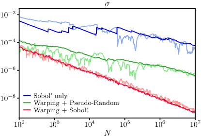
A more robust estimate of the error can be achieved by reintroducing a random component to the method – so-called Randomized Quasi-Monte Carlo Dick et al. (2013); Nuyens ; Dick and Pillichshammer (2010); L’Ecuyer (2018). Here we repeat the calculations with $K$ ‘randomly shifted’ sequences giving a distribution of values $Q_{k}$, from which we obtain an estimate of the mean and error as for conventional Monte Carlo. Typically one chooses only a moderate number of $K\sim 10-100$ as it is advantageous, for fixed computational time, to maximize $N$. In Fig. 7, we show this approach in practice for different methods of Fig. 4.

Figure 7: Absolute error of occupation number $Q_{6}(N)$, with curves matching three cases of Fig. 4. Here we perform calculations with $K=25$ shifted sequences. The pale curves show the convergence of the average over these runs to the Bethe ansatz result. The solid curves show the corresponding uncertainty estimates computed from the standard error of the mean over the shifted sequence values. We see that this procedure gives good estimates of the error.

Appendix H Details on the current $I$ calculation

This appendix gives details of the calculations made to obtain Fig. 3.

In this application, each lead has centered, semi-circular density of states with half-bandwidth $D=2$. The coupling to the leads is chosen so that $\Gamma=0.1$. A symmetric bias voltage $V$ is applied between the two leads. For each parameter set ($\varepsilon_{d},V,U$), $E_{d}$ and $\alpha$ are chosen so that the first order (Hartree term) of the perturbation series vanishes at $U=7\Gamma$, to improve its convergence radius. The series, defined in Appendix E, is computed at a time $t=10/\Gamma$ after switching the interaction on.

Due to the finite bandwidth $D$, the integrand decays polynomially at large times, but exponentially at intermediate times. We used an exponential warping with $\tau=1.5/\Gamma$, which was enough to capture the general shape of the integrand up to the observation time $t$.

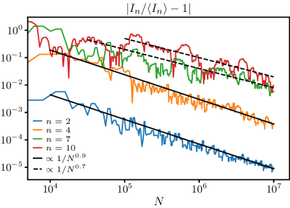
Figure 8 shows the convergence of the calculation for a system away from particle-hole symmetry ($E_{d}\approx 0.9\Gamma$, $\alpha\approx 0.27$, which in Fig. 3 corresponds to the point $\varepsilon_{d}/U\approx-0.12$ and $U=6\Gamma$). We observe a scaling slightly below $1/N$, which deteriorates with increasing order. Also, at large orders, the final scaling regime is reached at a later $N$.

Note that the data of Figs. 2, 4 and 8 have been smoothed for visibility: for $N>100$, we show the maximum of the error in a moving window around $N$ of fixed size in log-space ($5\%$ of $N$). This smoothing generates an upper bound of the error.

For each integration, digitally shifted Kuo and Nuyens (2016) generators are used to produce 10 different Sobol’ sequences from which we take the average to obtain the final result $\langle I_{n}\rangle$. The error is estimated by taking the standard deviation of the 10 results and dividing by $\sqrt{10}$. An example of a series computed with its estimated error is shown in Fig. 9. The error (black dots) on the coefficients (colored dots) is low enough so that only the truncation of the series limits the resummation accuracy.

The convergence radii of the series are about 3–4 $\Gamma$, so the series are resummed to obtain answers at larger interaction $U$. We use the conformal transform technique of Ref. Bertrand et al. (2019a) with the so-called parabola transform $W=-\tan^{2}(\sqrt{U/p})$. Here $p$ is a real negative parameter optimized for each series. Depending on their analytical structure, the series $I(U)$ or its inverse $1/I(U)$ is resummed, whichever gives smaller error. The integration error is propagated through the resummation process and added to the truncation error, the latter being estimated from the convergence radius of the resummed series. Unlike in Ref. Bertrand et al. (2019a), no Bayesian inference is used.

Figure 8: Convergence of the current $I_{n}$ with number of samples $N$ at different orders $n$. This data corresponds to a typical point of Fig. 3, away from particle-hole symmetry ($\varepsilon_{d}/U\approx-0.12$, $\alpha\approx 0.27$, $U=6\Gamma$). At low order (blue and orange lines) the relative error scales as $1/N^{0.9}$ (black plain line). At larger orders ($n=7$ and $10$, green and red lines), the convergence slows down and scales only as $1/N^{0.7}$ (dashed black line). Finally at order $n=10$, the final scaling starts at a larger number of function evaluations $N$ than for lower orders. For visibility, the data has been smoothed as described in Appendix H (see main text).

Figure 9: Perturbation series of the current for the same parameters as in Fig. 8. The upper line (colored symbols) gives the absolute values of the series coefficients $|I_{n}|$: positive coefficients are depicted in blue, and negative ones in red. The lower line (black symbols) is the estimated absolute error $\Delta I_{n}$. For all orders calculated, up to $n=10$, we obtained at least two digits of accuracy.

At large $\varepsilon_{d}$, the integrands become more difficult to integrate, but at the same time the summation of the series requires less orders for the same precision. When $\varepsilon_{d}/U>0.5$ (or $\varepsilon_{d}/U<-1.5$ by symmetry) we only computed and summed the series up to order $n=5$.

Finally, it is worth noting that small bias $V$ setups reach a stationary regime after a longer time. Hence performing the integration away from the linear response regime, at large $V$, is actually less expensive and less prone to sign problem. Physically, the voltage reduces the coherence of the system, which explains the reduction of almost exact cancellations in the numerical integration.

Appendix I Construction of the 1D Model Function

In this appendix, we explain how the $h^{(i)}$ functions are constructed in the model function defined in the main text,

$$p_{n}(\boldsymbol{u})=\prod_{i=1}^{n}h^{(i)}\bigl{(}u_{i-1}-u_{i}\bigr{)}.$$ (6^′)

for $0<u_{n}<u_{n-1}<\ldots<u_{2}<u_{1}$ and $u_{0}=t$ is defined to be the measurement time.

We are going to use successive changes of variable in this section:

$$\boldsymbol{u}\rightarrow\boldsymbol{v}\rightarrow\boldsymbol{w}\rightarrow\boldsymbol{x}$$ (31)

First, we change to the $v_{i}$ variables defined as $v_{i}\equiv u_{i-1}-u_{i}>0$ which are natural since the integrand only depends on time differences. The corresponding Jacobian is one. Note that the integration on $\boldsymbol{v}$ is performed on $[0,\infty)^{n}$. When going back to $\boldsymbol{u}$ space, this generates extra points that are not in the original $\boldsymbol{u}$ domain. The value of the integrand for these points is simply zero so that they induce no extra computational cost.

I.1 Exponential form for $h^{(i)}$

Our second change of variable $\boldsymbol{v}\rightarrow\boldsymbol{w}$ will be based on a model function with a simple analytic form for $h^{(i)}$, designed to correctly describe the asymptotics of the integrand. This asymptotic region becomes increasingly important at large order $n$, especially in the long time limit $t\rightarrow\infty$. We choose a simple form, independent of $i$

$$h^{(i)}_{\rm exp}(v)=e^{-v/\tau},\qquad\forall i.$$ (32)

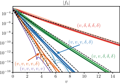
This choice is motivated by a direct study of the integrand. In Fig. 10, we plot the absolute value of the integrand $|f_{5}(v_{1},v_{2},v_{3},v_{4},v_{5})|$ of $Q_{5}$ with the parameters of our benchmark along various directions of the $5$ dimensional $\boldsymbol{v}$-space. The different colors correspond to different directions: red corresponds to $(v,\delta,\delta,\delta,\delta)$ where $\delta$ is fixed to $\delta=0.5$ and $v$ is varied. The 5 different curves correspond to different permutations of the $v$ with respect to the $\delta$. Green curves correspond to the 10 different permutations of $(v,v,\delta,\delta,\delta)$ and so on. The dashed line corresponds to Eq. (32) with $\tau=0.95$. Remarkably, such a simple ansatz with a single parameter, already captures the integrand asymptotics well, in various directions in 5 dimensions.

Figure 10: Comparison between the absolute value of the order 5 integrand $|f_{5}(\boldsymbol{v})|$ in Eq. (2) (colored lines) and the model function $p_{5}(\boldsymbol{v})$ of Eq. (6^′) (black dashed lines, $\tau=0.95$) along various directions in $\boldsymbol{v}$-space. Each color corresponds to $\boldsymbol{v}=(v,\ldots,\delta)$ as indicated in the figure. Lines of the same color correspond to different permutations within a given direction (see main text). The parameters are the same as in Fig. 1.

For a fixed number of integrand evaluations $N$, the error made in the calculation of $Q_{n}$ is very sensitive to the choice of the parameter $\tau$ as shown in Fig. 11. For $N=10^{6}$, Fig. 11 shows the relative error as a function of $\tau$ for various orders $n=5,6,7$ and $10$. The error possesses a sharp minimum around $\tau=0.85$ (note the log scale). If $\tau$ is too small, we under-sample the tails of the function leading to potentially incorrect results. If $\tau$ is too large, the calculation is correct, but less efficient since the sampling puts a lot of points in regions which contribute little to the result. We will now see how to make the computation more robust regarding the choice of $\tau$.

I.2 Learning $h^{(i)}$ from the integrand

In this section, we make an additional change of variable $\boldsymbol{w}\rightarrow\boldsymbol{x}$. To approximate the new integrand $\tilde{f}_{n}(\boldsymbol{w})$ in the $\boldsymbol{w}$ variable, we search for a new model function $\tilde{p}_{n}(\boldsymbol{w})$, again having the form:

$$\tilde{p}_{n}(\boldsymbol{w})=\prod_{i=1}^{n}\tilde{h}^{(i)}\bigl{(}w_{i}\bigr{)}.$$ (33)

If we assume that the integrand $\tilde{f}_{n}(\boldsymbol{w})$ is well approximated by such a simple form, we estimate the functions $\tilde{h}^{(i)}$ by projecting in each dimension

$$\tilde{h}^{(i)}_{\rm proj}(y)\equiv\int\mathrm{d}^{n}\boldsymbol{w}\tilde{f}_{n}(\boldsymbol{w})\delta(w_{i}-y).$$ (34)

In practice, we calculate $M$ values of the integrand $\tilde{f}(\boldsymbol{w}_{\alpha})$, $\alpha\in 1...M$ generated by sampling the $\boldsymbol{w}$ space using the Sobol’ sequence, and bin them in each dimension with $N_{b}$ bins. The function that we obtain is rather noisy due to the binning, so in a second step, we use a Gaussian kernel smoothing

$$\tilde{h}^{(i)}_{\rm proj}(w)\rightarrow\frac{\sum_{l=1}^{N_{b}}K_{\lambda}\left(w,\frac{l}{N_{b}}\right)\tilde{h}^{(i)}_{\rm proj}\left(\frac{l}{N_{b}}\right)}{\sum_{l=1}^{N_{b}}K_{\lambda}\left(w,\frac{l}{N_{b}}\right)}$$ (35)

where

$$K_{\lambda}(w,w^{\prime})=e^{{-(w-w^{\prime})^{2}/\lambda^{2}}}.$$ (36)

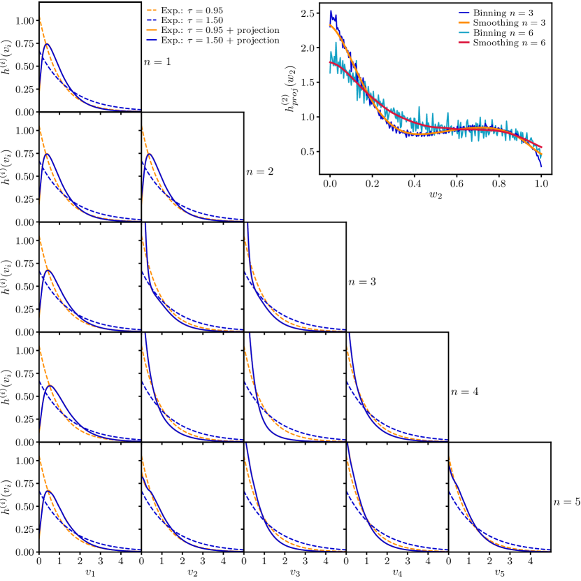
The upper right plot of Fig. 12 shows an example of the smoothing procedure.

Figure 11: Exact relative error of $Q_{n}$ computed with $N=10^{6}$ points as a function of the model function parameter $\tau$. The dashed lines are for a model defined by a single exponential function $h^{(i)}(v_{i})=\exp(-v_{i}/\tau)$, at different orders. The red solid curve is the new error after optimization of $h^{(i)}$ by projection (see section I.2), at order $n=7$. The parameters are the same as in Fig. 1.

Figure 12: Examples of functions $h^{(i)}(v_{i})$ for various $n$ and $1\leq i\leq n$: exponential form (dashed lines) and after projection (plain lines, on top of each other). We used $N_{b}=250$ bins, $M=20000$ samples and $\lambda=0.05$; see text. An example of binned values and smoothing for $h^{(2)}_{\rm proj}$ for order $n=3,6$ is shown in the upper right inset. The parameters are the same as in Fig. 1.

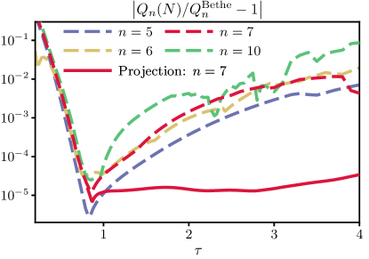
The change of variable based on $\tilde{h}^{(i)}_{\rm proj}$ was used to compute the continuous line in Fig. 11 for order $n=7$ ($N_{b}=100,M=10^{5},\lambda=0.05$). The error is improved at the optimum point $\tau=0.95$ only by approximately a factor 2. However, it remains largely independent of the value $\tau$ selected for the $\boldsymbol{v}\rightarrow\boldsymbol{w}$ change of variable, showing that the method has become much more robust. The projection automatically fits the exponential tails, without manual adjustment (as long as $\tau$ is not too small, to avoid under-sampling as explained above). Note that in Fig. 11, only $M=10^{5}$ values of the integrand were used for the learning step. This is 1% of the total number of function calls, hence negligible. If $\tau$ is increased, the sampling of the integrand decreases in quality, as the tails are over-sampled. Correcting this in the learning step becomes increasingly more demanding. Therefore the change of variable $\boldsymbol{v}\rightarrow\boldsymbol{w}$ with a good initial guess for $\tau$ is essential to the success of the projection.

Because we only used model functions of the form Eq. (6^′), according to Eq. (14), $x_{m}$ only depends on $w_{m}$, which itself only depends on $v_{m}$. In this special situation, the change of variable $\boldsymbol{v}\rightarrow\boldsymbol{x}$ can be represented by a model function of the form Eq. (6^′), and compared to the simpler $\boldsymbol{v}\rightarrow\boldsymbol{w}$. As a result, Fig. 12 shows $h^{(i)}_{\rm proj}(v_{i})$ along with the initial exponential guess, for all $i$ and $n\leq 5$, and for two values of $\tau=0.95$ and $\tau=1.5$. $h^{(i)}_{\rm proj}$ computed from two different initial guess for $\tau$ are indistinguishable (plain lines, on top of each other), showing that the result is independent of the initial choice of $\tau$. At small $v$, they are quite different from a pure exponential. Finally, we note that the projected model functions vary only slightly with $n$ for most values of $i$. This could be turned into an advantage by reusing the $h$ functions from a lower dimension to a higher one in future developments.

I.3 Comparison to VEGAS algorithm

The form of model function Eq. (6^′) and the projection procedure described above are related to the VEGAS algorithm Lepage (1978, 1980). However, simply applying this algorithm to perform the perturbation theory integrals produces poor results. Here we describe the essential differences between VEGAS and our approach.

The standard VEGAS algorithm uses random numbers to sample the integrand. It generates a weight function by projecting samples onto coordinate axes, which is analogous to the procedure we described. During the sampling steps, VEGAS uses the information it obtained to continuously improve the weight function.

To have a meaningful comparison, we will add physics information in the form of the $\boldsymbol{u}\to\boldsymbol{v}$ coordinate mapping (see above). The form Eq. (6^′) is only a good approximation to our integrand in the $\boldsymbol{v}$ variables. Although in our case VEGAS converges poorly in both $\boldsymbol{u}$ and $\boldsymbol{v}$ variables, it is far worse in $\boldsymbol{u}$.

Our approach still differs from VEGAS in two essential ways. First, a key feature of our approach is to correctly capture the decaying asymptotic structure in the model function analytically. As we have shown in Fig. 11, a pure projection method is prohibitively inefficient in sampling the long tails and leads to poor convergence. It is only useful as a small correction to a good starting point. Second, the continuous change of model function of VEGAS cannot be used together with low-discrepancy sequences, since it breaks their special properties. For QQMC to work and achieve $1/N$ convergence, it is essential to construct the model function entirely before the full calculation is performed. Samples cannot be “reused” as in Monte Carlo sampling. This again requires an numerically efficient way to construct the model function which is not a priori provided by VEGAS.

Finally, we note that the idea of the model function is more general than the product form of Eq. (6^′) and VEGAS. Although they were sufficient for the Anderson impurity model calculations presented here, more general model function such as an MPS Eq. (7) are important for more complex many-body systems.

References

- Gross and Bloch (2017) Christian Gross and Immanuel Bloch, “Quantum simulations with ultracold atoms in optical lattices,” Science 357, 995 (2017).
- Blatt and Roos (2012) R. Blatt and C. F. Roos, “Quantum simulations with trapped ions,” Nature Phys 8, 277 (2012).
- Goldhaber-Gordon et al. (1998a) D. Goldhaber-Gordon, Hadas Shtrikman, D. Mahalu, David Abusch-Magder, U. Meirav, and M. A. Kastner, “Kondo effect in a single-electron transistor,” Nature 391, 156 (1998a).
- Goldhaber-Gordon et al. (1998b) D. Goldhaber-Gordon, J. Göres, M. A. Kastner, Hadas Shtrikman, D. Mahalu, and U. Meirav, “From the Kondo regime to the mixed-valence regime in a single-electron transistor,” Phys. Rev. Lett. 81, 5225–5228 (1998b).
- Cronenwett et al. (1998) Sara M. Cronenwett, Tjerk H. Oosterkamp, and Leo P. Kouwenhoven, “A tunable Kondo effect in quantum dots,” Science 281, 540–544 (1998).
- Iftikhar et al. (2018) Z. Iftikhar, A. Anthore, A. K. Mitchell, F. D. Parmentier, U. Gennser, A. Ouerghi, A. Cavanna, C. Mora, P. Simon, and F. Pierre, “Tunable quantum criticality and super-ballistic transport in a “charge” Kondo circuit,” Science 360, 1315 (2018).
- Bernien et al. (2017) Hannes Bernien, Sylvain Schwartz, Alexander Keesling, Harry Levine, Ahmed Omran, Hannes Pichler, Soonwon Choi, Alexander S. Zibrov, Manuel Endres, Markus Greiner, Vladan Vuletić, and Mikhail D. Lukin, “Probing many-body dynamics on a 51-atom quantum simulator,” Nature 551, 579 (2017).
- LeBlanc et al. (2015) J. P. F. LeBlanc, Andrey E. Antipov, Federico Becca, Ireneusz W. Bulik, Garnet Kin-Lic Chan, Chia-Min Chung, Youjin Deng, Michel Ferrero, Thomas M. Henderson, Carlos A. Jiménez-Hoyos, E. Kozik, Xuan-Wen Liu, Andrew J. Millis, N. V. Prokof’ev, Mingpu Qin, Gustavo E. Scuseria, Hao Shi, B. V. Svistunov, Luca F. Tocchio, I. S. Tupitsyn, Steven R. White, Shiwei Zhang, Bo-Xiao Zheng, Zhenyue Zhu, and Emanuel Gull (Simons Collaboration on the Many-Electron Problem), “Solutions of the two-dimensional Hubbard model: Benchmarks and results from a wide range of numerical algorithms,” Phys. Rev. X 5, 041041 (2015).
- Cohen et al. (2015) Guy Cohen, Emanuel Gull, David R. Reichman, and Andrew J. Millis, “Taming the dynamical sign problem in real-time evolution of quantum many-body problems,” Phys. Rev. Lett. 115, 266802 (2015).
- Profumo et al. (2015) Rosario E. V. Profumo, Christoph Groth, Laura Messio, Olivier Parcollet, and Xavier Waintal, “Quantum Monte Carlo for correlated out-of-equilibrium nanoelectronic devices,” Phys. Rev. B 91, 245154 (2015), arXiv:1504.02132 .
- Bertrand et al. (2019a) Corentin Bertrand, Serge Florens, Olivier Parcollet, and Xavier Waintal, “Reconstructing nonequilibrium regimes of quantum many-body systems from the analytical structure of perturbative expansions,” Phys. Rev. X 9, 041008 (2019a), arXiv:1903.11646 .
- Prokof’ev and Svistunov (1998) Nikolai V. Prokof’ev and Boris V. Svistunov, “Polaron problem by diagrammatic quantum Monte Carlo,” Phys. Rev. Lett. 81, 2514 (1998), arXiv:cond-mat/9804097 .
- Prokof’ev and Svistunov (2008) N. V. Prokof’ev and B. V. Svistunov, “Bold diagrammatic Monte Carlo: A generic sign-problem tolerant technique for polaron models and possibly interacting many-body problems,” Phys. Rev. B 77, 125101 (2008), arXiv:0801.0911 .
- Mishchenko et al. (2001) A. S. Mishchenko, N. V. Prokof’ev, B. V. Svistunov, and A. Sakamoto, “Comprehensive study of Fröhlich polaron,” Int. J. Mod. Phys. B 15, 3940–3943 (2001).
- Van Houcke et al. (2012) K. Van Houcke, F. Werner, E. Kozik, N. Prokof’ev, B. Svistunov, M. J. H. Ku, A. T. Sommer, L. W. Cheuk, A. Schirotzek, and M. W. Zwierlein, “Feynman diagrams versus Fermi-gas Feynman emulator,” Nature Phys 8, 366 (2012), arXiv:1110.3747 .
- Wu et al. (2017) Wei Wu, Michel Ferrero, Antoine Georges, and Evgeny Kozik, “Controlling Feynman diagrammatic expansions: Physical nature of the pseudogap in the two-dimensional Hubbard model,” Phys. Rev. B 96, 041105 (2017), arXiv:1608.08402 .
- Rossi (2017) Riccardo Rossi, “Determinant diagrammatic Monte Carlo algorithm in the thermodynamic limit,” Phys. Rev. Lett. 119, 045701 (2017), arXiv:1612.05184 .
- Chen and Haule (2019) Kun Chen and Kristjan Haule, “A combined variational and diagrammatic quantum Monte Carlo approach to the many-electron problem,” Nat Commun 10, 3725 (2019), arXiv:1809.04651 .
- Bertrand et al. (2019b) Corentin Bertrand, Olivier Parcollet, Antoine Maillard, and Xavier Waintal, “Quantum Monte Carlo algorithm for out-of-equilibrium Green’s functions at long times,” Phys. Rev. B 100, 125129 (2019b), arXiv:1903.11636 .
- Moutenet et al. (2019) Alice Moutenet, Priyanka Seth, Michel Ferrero, and Olivier Parcollet, “Cancellation of vacuum diagrams and the long-time limit in out-of-equilibrium diagrammatic quantum Monte Carlo,” Phys. Rev. B 100, 085125 (2019), arXiv:1904.11969 .
- (21) Riccardo Rossi, Fedor Simkovic, and Michel Ferrero, “Renormalized perturbation theory at large expansion orders,” arXiv:2001.09133 .
- Dick et al. (2013) Josef Dick, Frances Y. Kuo, and Ian H. Sloan, “High-dimensional integration: The quasi-Monte Carlo way,” Acta Numer. 22, 133 (2013).
- (23) Dirk Nuyens, “The construction of good lattice rules and polynomial lattice rules,” arXiv:1308.3601 .
- Dick and Pillichshammer (2010) Josef Dick and Friedrich Pillichshammer, Digital Nets and Sequences: Discrepancy Theory and Quasi–Monte Carlo Integration (Cambridge University Press, Cambridge, 2010).
- L’Ecuyer (2018) Pierre L’Ecuyer, “Randomized quasi-Monte Carlo: An introduction for practitioners,” in Monte Carlo and Quasi-Monte Carlo Methods, edited by Art B. Owen and Peter W. Glynn (Springer International Publishing, Cham, 2018) pp. 29–52.
- Sobol’ (1967) I.M Sobol’, “On the distribution of points in a cube and the approximate evaluation of integrals,” USSR Computational Mathematics and Mathematical Physics 7, 86 (1967).
- Kuo and Nuyens (2016) Frances Y. Kuo and Dirk Nuyens, “Application of quasi-Monte Carlo methods to elliptic pdes with random diffusion coefficients: A survey of analysis and implementation,” Found Comput Math 16, 1631 (2016).
- Tsvelick and Wiegmann (1983) A.M. Tsvelick and P.B. Wiegmann, “Exact results in the theory of magnetic alloys,” Advances in Physics 32, 453 (1983).
- Okiji and Kawakami (1984) Ayao Okiji and Norio Kawakami, “Thermodynamic properties of the Anderson model (invited),” Journal of Applied Physics 55, 1931 (1984).
- Tans et al. (1997) Sander J. Tans, Michel H. Devoret, Hongjie Dai, Andreas Thess, Richard E. Smalley, L. J. Geerligs, and Cees Dekker, “Individual single-wall carbon nanotubes as quantum wires,” Nature 386, 474 (1997).
- Nygård et al. (2000) Jesper Nygård, David Henry Cobden, and Poul Erik Lindelof, “Kondo physics in carbon nanotubes,” Nature 408, 342 (2000).
- Liang et al. (2001) Wenjie Liang, Marc Bockrath, Dolores Bozovic, Jason H. Hafner, M. Tinkham, and Hongkun Park, “Fabry - Perot interference in a nanotube electron waveguide,” Nature 411, 665 (2001).
- Roch et al. (2008) Nicolas Roch, Serge Florens, Vincent Bouchiat, Wolfgang Wernsdorfer, and Franck Balestro, “Quantum phase transition in a single-molecule quantum dot,” Nature 453, 633 (2008).
- Ridley et al. (2019) Michael Ridley, Michael Galperin, Emanuel Gull, and Guy Cohen, “Numerically exact full counting statistics of the energy current in the Kondo regime,” Phys. Rev. B 100, 165127 (2019), arXiv:1907.09546 .
- Krivenko et al. (2019) Igor Krivenko, Joseph Kleinhenz, Guy Cohen, and Emanuel Gull, “Dynamics of Kondo voltage splitting after a quantum quench,” Phys. Rev. B 100, 201104 (2019), arXiv:1904.11527 .
- Beenakker (1991) C. W. J. Beenakker, “Theory of Coulomb-blockade oscillations in the conductance of a quantum dot,” Phys. Rev. B 44, 1646 (1991).
- Hofheinz et al. (2007) M. Hofheinz, X. Jehl, M. Sanquer, G. Molas, M. Vinet, and S. Deleonibus, “Capacitance enhancement in Coulomb blockade tunnel barriers,” Phys. Rev. B 75, 235301 (2007).
- Schollwöck (2011) Ulrich Schollwöck, “The density-matrix renormalization group in the age of matrix product states,” Annals of Physics 326, 96 (2011), arXiv:1008.3477 .
- (39) Ivan Glasser, Ryan Sweke, Nicola Pancotti, Jens Eisert, and J. Ignacio Cirac, “Expressive power of tensor-network factorizations for probabilistic modeling, with applications from hidden Markov models to quantum machine learning,” arXiv:1907.03741 .
- Parcollet et al. (2015) Olivier Parcollet, Michel Ferrero, Thomas Ayral, Hartmut Hafermann, Igor Krivenko, Laura Messio, and Priyanka Seth, “TRIQS: A toolbox for research on interacting quantum systems,” Computer Physics Communications 196, 398 – 415 (2015).
- Roth (1954) K. F. Roth, “On irregularities of distribution,” Mathematika 1, 73–79 (1954).
- Weyl (1916) Hermann Weyl, “Über die Gleichverteilung von Zahlen mod. Eins,” Mathematische Annalen 77, 313–352 (1916).
- Korobov (1957) N. M. Korobov, “Approximate calculation of repeated integrals by number-theoretical methods,” Doklady Akademii Nauk SSSR 115, 1062–1065 (1957).
- Hammersley (1960) J. M. Hammersley, “Monte Carlo methods for solving multivariable problems,” Annals of the New York Academy of Sciences 86, 844–874 (1960).
- van der Corput (1935) J. C. van der Corput, “Verteilungsfunktionen,” Nederl. Akad. Wetensch. Proc. 38, 813–821, 1058–1066 (1935).
- Halton (1960) J. H. Halton, “On the efficiency of certain quasi-random sequences of points in evaluating multi-dimensional integrals,” Numerische Mathematik 2, 84–90 (1960).
- Haselgrove (1961) C. B. Haselgrove, “A method for numerical integration,” Mathematics of Computation 15, 323–337 (1961).
- Richtmyer (1952) R D Richtmyer, The evaluation of definite integrals, and a quasi-Monte-Carlo method based on the properties of algebraic numbers, Tech. Rep. LA-1342 (Los Alamos Scientific Lab., Los Alamos, NM, 1952).
- Niederreiter (1978) Harald Niederreiter, “Quasi-Monte Carlo methods and pseudo-random numbers,” Bulletin of the American Mathematical Society 84, 957–1041 (1978).
- Conroy (1967) Harold Conroy, “Molecular Schrödinger equation. VIII. A new method for the evaluation of multidimensional integrals,” The Journal of Chemical Physics 47, 5307–5318 (1967).
- Berblinger and Schlier (1991) Michael Berblinger and Christoph Schlier, “Monte Carlo integration with quasi-random numbers: some experience,” Computer Physics Communications 66, 157–166 (1991).
- Paskov and Traub (1995) Spassimir H. Paskov and Joseph F. Traub, “Faster Valuation of Financial Derivatives,” J. Portf. Manag. 22, 113–123 (1995).
- Wang and Sloan (2005) Xiaoqun Wang and Ian H. Sloan, “Why are high-dimensional finance problems often of low effective dimension?” SIAM Journal on Scientific Computing 27, 159–183 (2005).
- Nuyens and Cools (2006) Dirk Nuyens and Ronald Cools, “Fast algorithms for component-by-component construction of rank-1 lattice rules in shift-invariant reproducing kernel Hilbert spaces,” Mathematics of Computation 75, 903–920 (2006).
- Lepage (1978) G. Peter Lepage, “A new algorithm for adaptive multidimensional integration,” Journal of Computational Physics 27, 192 (1978).
- Lepage (1980) G. Peter Lepage, VEGAS - an adaptive multi-dimensional integration program, Tech. Rep. CLNS-447 (Cornell Univ. Lab. Nucl. Stud., Ithaca, NY, 1980).
- Rubtsov and Lichtenstein (2004) A. N. Rubtsov and A. I. Lichtenstein, “Continuous-time quantum Monte Carlo method for fermions: Beyond auxiliary field framework,” Journal of Experimental and Theoretical Physics Letters 80, 61–65 (2004).
- Meir and Wingreen (1992) Yigal Meir and Ned S. Wingreen, “Landauer formula for the current through an interacting electron region,” Phys. Rev. Lett. 68, 2512–2515 (1992).
- Wiegmann and Tsvelick (1983) P B Wiegmann and A M Tsvelick, “Exact solution of the Anderson model: I,” J. Phys. C: Solid State Phys. 16, 2281 (1983).
- Horvatić and Zlatić (1985) B. Horvatić and V. Zlatić, “Equivalence of the perturbative and Bethe-Ansatz solution of the symmetric Anderson Hamiltonian,” J. Phys. France 46, 1459–1467 (1985).