Theoretical Models of Learning to Learn*

Abstract

A Machine can only learn if it is biased in some way. Typically the bias is supplied by hand, for example through the choice of an appropriate set of features. However, if the learning machine is embedded within an environment of related tasks, then it can learn its own bias by learning sufficiently many tasks from the environment [4, 6]. In this paper two models of bias learning (or equivalently, learning to learn) are introduced and the main theoretical results presented. The first model is a PAC-type model based on empirical process theory, while the second is a hierarchical Bayes model.

Department of Systems Engineering Research School of Information Science and Engineering Australian National University Canberra 0200 Australia

Keywords: Learning to Learn, Bias Learning, Empirical Processes, Hierarchical Bayes

1 Introduction

Hume’s analysis [10] shows that there is no a priori basis for induction. In a machine learning context, this means that a learner must be biased in some way for it to generalise well [11]. Typically such bias is introduced by hand through the skill and insights of experts, but despite many notable successes, this process is limited by the experts’ abilities. Hence a desirable goal is to find ways of automatically learning the bias. Bias learning is a form of learning to learn, and the two expressions will be used interchangeably throughout this document.

The purpose of this chapter is to present an overview of two models of supervised bias learning. The first [4, 3] is based on Empirical Process theory (henceforth the EP model) and the second [6] is based on Bayesian inference and information theory (henceforth the Bayes model). Empirical process theory is a general theory that includes the analysis of pattern classification first introduced by Vapnik and Chervonenkis [13, 12]. Note that these are models of supervised bias learning and as such have little to say about learning to learn in a reinforcement learning setting.

In this introduction a high level overview of the features common to both models will be presented, and then in later sections the details and main results of each model will be discussed.

In ordinary models of machine learning the learner is presented with a single task. Learning the “right bias” in such a model does not really make sense, because the ultimate bias is one which completely solves the task. Thus in single-task learning, bias learning or learning to learn is the same as learning.

In order to learn bias one has introduce extra assumptions about the learning process. The central assumption of both the Bayes model and the EP model of bias learning is that the learner is embedded within an environment of related problems. The learner’s task is to find a bias that is appropriate for the entire environment, not just for a single task.

A simple example of an environment of learning problems with a common bias is handwritten character recognition. A preprocessing stage that identifies and removes any (small) rotations, dilations and translations of an image of a character will be advantageous for recognising all characters. If the set of all individual character recognition problems is viewed as an environment of learning tasks, this preprocessor represents a bias that is appropriate to all tasks in the environment.

Preprocessing can also be viewed as feature extraction, and there are many classes of learning problems that possess common feature sets. For example, one can view face recognition as a collection of related learning problems, one for each possible face classifier, and it is likely that there exists sets of features that are good for learning all faces. A similar conclusion applies to other domains such as speech recognition (all the individual word classifiers may be viewed as separate learning problems possessing a common feature set), fingerprint recognition, and so on. The classical approach to statistical pattern recognition in these domains is to first guess a set of features and then to learn each problem by estimating a simple (say linear) function of the features. The choice of features represents the learner’s bias, thus in bias learning the goal is to get the learner to learn the features instead of guessing them.

In order to perform a theoretical analysis of bias learning, we assume the tasks in the environment are generated according to some underlying probability distribution. For example, if the learner is operating in an environment where it must learn to recognise faces, the distribution over learning tasks will have its support restricted to face recognition type problems. The learner acquires information about the environment by sampling from this distribution to generate multiple learning problems, and then sampling from each learning problem to generate multiple training sets. The learner can then search for bias that is appropriate for learning all the tasks.

In the EP model, the learner is provided with a family of hypothesis spaces and it searches for an hypothesis space that contains good solutions to all the training sets. Such a hypothesis space can then be used to learn novel tasks drawn from the same environment. The key result of the EP model (theorem 2 in section 3) gives a bound on the number of tasks and number of examples of each task required to ensure that a hypothesis space containing good solutions to all training sets will, with high probability, contain good solutions to novel tasks drawn from the same environment. This ability to learn novel tasks after seeing sufficiently many examples of sufficiently many tasks is the formal definition of learning to learn under the EP model.

The Bayes model is the same as the EP model in that the learner is assumed to be embedded within an environment of related tasks and can sample from the environment to generate multiple training sets corresponding to different tasks. However, the Bayes bias learner differs in the way it uses the information from the multiple training sets. In the Bayes model, the distribution over learning tasks in the environment is interpreted as an objective prior distribution. The learner does not know this distribution, but does have some idea of a set $\Pi$ of possible prior distributions to which the true distribution belongs. The learner starts out with a hyper-prior distribution on $\Pi$ and based on the data in the training sets, updates the hyper-prior to a hyper-posterior using Bayes’ rule. The hyper-posterior is then used as a prior distribution when learning novel tasks. In section 4 results will be presented showing how the information needed to learn each task (in a Shannon sense) decays to the minimum possible for the environment as the number of tasks and number of examples of each tasks seen already grows. Within the Bayes model, this is the formal definition of learning to learn.

Before moving on to the details of these models, it is worth pausing to assess what bias learning solves, and what it doesn’t—and in a sense can never—solve. On face value, being able to learn the right bias appears to violate Hume’s conclusion that there can be no a priori basis for induction. However this is not the case, for the bias learner learner is still fundamentally limited by the possible choices of bias available. For example, if a learner is learning a set of features for an environment in which there are in fact no small feature sets, then any bias it comes up with (i.e. any feature set) will be a very poor bias for that environment. Thus, there is still guesswork involved in determining the appropriate way to hyper-bias the learner. The main advantage of bias learning is that this hyper-bias can be much weaker than the bias: the right hyper-bias for many environments is just that there exists a set of features, whereas specifying the right bias means actually finding the features.

2 Statistical Models of Ordinary Learning

To understand how bias learning can be modeled from a statistical perspective, it is necessary to first understand how ordinary learning is modeled from a statistical perspective. The empirical process (EP) process approach and the Bayes approach will be discussed in turn.

2.1 The empirical process (EP) approach

The empirical process (EP) approach to modeling ordinary (single-task) learning has the following essential ingredients:

• An input space $X$ and an output space $Y$,

• a probability distribution $P$ on $X\times Y$,

• a loss function $l\colon Y\times Y\to{R}$, and

• a hypothesis space ${\cal H}$ which is a set of hypotheses or functions $h\colon X\to Y$.

As an example, if the problem is to learn to recognize images of Mary’s face using a neural network, then $X$ would be the set of all images (typically represented as a subset of ${R}^{d}$ where each component is a pixel intensity), $Y$ would be the set $\{0,1\}$, and the distribution $P$ would be peaked over images of different faces and the correct class labels. The learner’s hypothesis space ${\cal H}$ would be a class of neural networks mapping the input space (${R}^{d}$) to $\{0,1\}$.

$$l(y,y^{\prime}):=\left\{\begin{array}[]{ll}1&\mbox{if $y\neq y^{\prime}$}\\ 0&\mbox{if $y=y^{\prime}$}\end{array}\right.$$ (1)

Using the loss function allows us to present a unified treatment of both concept learning ($Y=\{0,1\}$, $l$ as above), and real-valued function learning (e.g. regression) in which $Y={R}$ and $l(y,y^{\prime})=(y-y^{\prime})^{2}$.

The goal of the learner is to select a hypothesis $h\in{\cal H}$ with minimum expected loss:

$${\mbox{er}}_{P}(h):=\int_{X\times Y}l(h(x),y)\,dP(x,y).$$ (2)

For classifying Mary’s face, the $h\in{\cal H}$ with minimum value of ${\mbox{er}}_{P}(h)$ is the one that makes the fewest number of mistakes on average. Of course, the learner does not know $P$ and so it cannot search through ${\cal H}$ for an $h$ minimizing ${\mbox{er}}_{P}(h)$. In practice, the learner samples repeatedly from the distribution $P$ to generate a training set

$$z:=\{(x_{1},y_{1}),\dots,(x_{m},y_{m})\},$$ (3)

and instead of minimizing ${\mbox{er}}_{P}(h)$, the learner searches for an $h\in{\cal H}$ minimizing the empirical loss on sample $z$:

$${\hat{{\mbox{er}}}}_{z}(h):=\frac{1}{m}\sum_{i=1}^{m}l(h(x_{i}),y_{i}).$$ (4)

Of course, there are more intelligent things to do with the data than simply minimizing empirical error—for example one can add regularisation terms to avoid over-fitting. However we do not consider those issues here as they do not substantially alter the discussion.

Minimizing ${\hat{{\mbox{er}}}}_{z}(h)$ is only a sensible thing to do if there is some guarantee that ${\hat{{\mbox{er}}}}_{z}(h)$ is close to expected loss ${\mbox{er}}_{P}(h)$. This will in turn depend on the “richness” of the class ${\cal H}$ and the size of the training set ($m$). If ${\cal H}$ contains every possible function then clearly there can never be any guarantee that ${\hat{{\mbox{er}}}}_{z}(h)$ is close to ${\mbox{er}}_{P}(h)$. The conditions ensuring convergence between ${\hat{{\mbox{er}}}}_{z}(h)$ and ${\mbox{er}}_{P}(h)$ are by now well understood; in the case Boolean function learning ($Y=\{0,1\}$), convergence is controlled by ${\mbox{VCdim}}({\cal H})$—the VC-dimension of ${\cal H}$ (see e.g. [1, 12]). The following is typical of the theorems in this area.

Theorem 1

Let $P$ be any probability distribution on $X\times\{0,1\}$ and suppose $z=\{(x_{1},y_{1}),\dots,(x_{m},y_{m})\}$ is generated by sampling $m$ times from $X\times\{0,1\}$ according to $P$. Let $d:={\mbox{VCdim}}({\cal H})$. Then with probability at least $1-\delta$ (over the choice of the training set $z$), all $h\in{\cal H}$ will satisfy

$${\mbox{er}}_{P}(h)\leq{\hat{{\mbox{er}}}}_{z}(h)+\left[\frac{32}{m}\left(d\ln\frac{2em}{d}+\ln\frac{4}{\delta}\right)\right]^{1/2}$$ (5)

There are a number of key points about this theorem:

1. We can never say for certain that ${\mbox{er}}_{P}(h)$ and ${\hat{{\mbox{er}}}}_{z}(h)$ are close, only that they are close with high probability ($1-\delta$). This is because no matter how large the training set, there is always a chance that we will get unlucky and generate a highly unrepresentative sample $z$.

2. Keeping the confidence parameter $\delta$ fixed, and ignoring $\log$ factors, (5) shows that the difference between the empirical estimate ${\hat{{\mbox{er}}}}_{z}(h)$ and the true loss ${\mbox{er}}_{P}(h)$ decays like $\sqrt{d/m}$, uniformly for all $h\in{\cal H}$. Thus, for sufficiently large training sets $z$ and if $d={\mbox{VCdim}}({\cal H})$ is finite, we can be confident that an $h$ with small empirical error will generalise well.

3. If ${\cal H}$ contains an $h$ with zero error, and the learner always chooses an $h$ consistent with the training set, then the rate of convergence of ${\hat{{\mbox{er}}}}_{z}(h)$ and ${\mbox{er}}_{P}(h)$ can be improved to $d/m$.

4. Often results such as theorem 1 are called uniform convergence results, because they provide bounds for all $h\in{\cal H}$.

Theorem 1 only provides conditions under which the deviation between ${\mbox{er}}_{P}(h)$ and ${\hat{{\mbox{er}}}}_{z}$ is small, it does not guarantee that the true error ${\mbox{er}}_{P}(h)$ will actually be small. This is governed by the choice of ${\cal H}$. If ${\cal H}$ contains a solution with small error and the learner minimizes error on the training set, then with high probability ${\mbox{er}}_{P}(h)$ will be small. However, a bad choice of ${\cal H}$ will mean there is no hope of achieving small error. Thus, the bias of the learner in the EP model is represented by the choice of ${\cal H}$.

2.2 The Bayes approach

The Bayes approach and the EP approach are not all that different. In fact, the EP approach can be understood as a maximum likelihood approximation to the Bayes solution. The essential ingredients of the Bayes approach to modeling ordinary (single-task) learning are:

• An input space $X$ and an output space $Y$,

• a set of probability distributions $P_{\theta}$ on $X\times Y$, parameterised by $\theta\in\Theta$, and

• a prior distribution $p(\theta)$ on $\Theta$.

The hypothesis space ${\cal H}$ of the EP model has been replaced with a set of distributions $\{P_{\theta}\colon\theta\in\Theta\}$. As with the EP model, the learning task is represented by a distribution $P_{\theta^{*}}$ on $X\times Y$, only this time we assume realizability, i.e. that $\theta^{*}\in\Theta$. The prior distribution $p(\theta)$ represents the learner’s initial beliefs about the relative plausibility of each $P_{\theta}$. The richness of the set $\{P_{\theta}\colon\theta\in\Theta\}$ and the prior $p(\theta)$ represent the bias of the learner.

Again the learner does not know $\theta^{*}$, but has access to a training set $z=\{(x_{1},y_{1}),\dots,(x_{m},y_{m})\}$ of pairs $(x_{i},y_{i})$ sampled according to $P_{\theta^{*}}$. Upon receipt of the data $z$, the learner updates its prior distribution $p(\theta)$ to a posterior distribution $p(\theta|z)$ using Bayes rule:

$$p(\theta|z) := \frac{p(z|\theta)p(\theta)}{p(z)}$$

$$= \frac{\prod_{i=1}^{m}p(x_{i},y_{i}|\theta)p(\theta)}{\int_{\Theta}p(z|\theta)p(\theta)\,d\theta}.$$

Often we are not interested in modeling the input distribution, only the conditional distribution on $Y$ given $X$. In that case, $p(x,y|\theta)$ will factor into $p(x)p(y|x;\theta)$. The posterior distribution $p(\theta|z)$ can be used to predict the output $y$ of a novel input $x^{*}$ by averaging:

$$p(y|x^{*};z):=\int_{\Theta}p(y|x^{*};\theta)p(\theta|z)\,d\theta.$$ (7)

One would hope that as the data increases, predictions made in this way would become increasingly accurate. There are many ways to measure what we mean by “accurate” in this setting. The one considered here is the Kullback-Liebler (KL) divergence between the true distribution $P_{\theta^{*}}$ on $X\times Y$, and the posterior distribution $P_{m}$ on $X\times Y$ with density

$$p(x,y|z):=\int_{\Theta}p(x,y|\theta)p(\theta|z)\,d\theta.$$ (8)

The KL divergence between $P_{\theta^{*}}$ and $P_{m}$ is defined to be

$$D_{K}(P_{\theta}^{*}\|P_{m}):=\int_{X\times Y}p(x,y|\theta^{*})\log\frac{p(x,y|\theta^{*})}{p(x,y|z)}\,dx\,dy$$ (9)

Note that if $p(x,y|\theta)=p(x)p(y|\theta)$ as above then

$$D_{K}(P_{\theta}^{*}\|P_{m})=\int_{X\times Y}p(x)p(y|x;\theta^{*})\log\frac{p(y|x;\theta^{*})}{p(y|x;z)}\,dx\,dy.$$ (10)

This form of the KL divergence has a natural interpretation: it is (within one bit) the expected extra number of bits needed to encode the output $y$ using a code generated by the posterior $p(y|x;z)$, over and above what would be required using an optimal code (one generated from $p(y|x;\theta^{*})$). The expectation is over all pairs $(x,y)$ drawn according to the true distribution $P_{\theta^{*}}$. This quantity is only zero if the posterior is equal to the true distribution.

In [8, 2] an analysis of $D_{K}(P_{\theta^{*}}\|P_{m})$ was given for the limit of large training set size $(m)$. They showed that if $\Theta$ is a compact subset of ${R}^{d}$, and under certain extra restrictions which we won’t discuss here:

$$D_{K}(P_{\theta^{*}}\|P_{m})=\frac{d}{m}+o\left(\frac{1}{m}\right)$$ (11)

where $o(1/m)$ stands for a function $f(m)$ for which $mf(m)\rightarrow 0$ as $m\rightarrow\infty$.

There is a strong similarity between this result and theorem 1 in the zero error case (see note 3 after the theorem). $D_{K}(P_{\theta^{*}}\|P_{m})$ is the analogue of $|{\mbox{er}}_{z}(h)-{\mbox{er}}_{P}(h)|$ in this case, but because we have assumed realizability, ${\mbox{er}}_{z}(h)=0$. So theorem 1 says that choosing any hypothesis consistent with the data will guarantee you an error of no more than $d/m$, where $d$ is the VC dimension of the learner’s hypothesis space. Although the error measure is different, equation (11) says essentially the same thing: if you classify novel data using a posterior generated according to Bayes rule, you will suffer an error of no more than $d/m$, where now $d$ is the dimension of the $\Theta$.

3 The empirical process (EP) model of learning to learn

Recall from the introduction that the main extra assumption of both the Bayes and EP models of bias learning is that the learner is embedded in an environment of related tasks, and can sample from the environment to generate multiple training sets belonging to multiple different tasks. In the EP model of ordinary (single-task) learning, the learning problem is represented by a distribution $P$ on $X\times Y$. So in the EP model of bias learning, an environment of learning problems is represented by a pair $({\cal P},Q)$ where ${\cal P}$ is the set of all probability distributions on $X\times Y$ (i.e. ${\cal P}$ is the set of all possible learning problems), and $Q$ is a distribution on ${\cal P}$. $Q$ controls which learning problems the learner is likely to see. For example, if the learner is in a face recognition environment, $Q$ will be highly peaked over face-recognition-type problems, whereas if the learner is in a character recognition environment $Q$ will be peaked over character-recognition-type problems.

Recall from the end of section 2.1 that the learner’s bias is represented by its choice of hypothesis space ${\cal H}$. So to enable the learner to learn the bias, it is supplied with a family or set of hypothesis spaces ${\mbox{\boldmath$\bf H$}}:=\{{\cal H}\}$. As each ${\cal H}$ is itself a set of functions $h\colon X\to Y$, $\bf H$ is a set of sets of functions.

Putting this together, formally a learning to learn or bias learning problem consists of:

• an input space $X$ and an output space $Y$,

• a loss function $l\colon Y\times Y\to{R}$,

• an environment $({\cal P},Q)$ where ${\cal P}$ is the set of all probability distributions on $X\times Y$ and $Q$ is a distribution on ${\cal P}$,

• a hypothesis space family ${\mbox{\boldmath$\bf H$}}=\{{\cal H}\}$ where each ${\cal H}\in{\mbox{\boldmath$\bf H$}}$ is a set of functions $h\colon X\to Y$.

The goal of a bias learner is to find a hypothesis space ${\cal H}\in{\mbox{\boldmath$\bf H$}}$ minimizing the loss (recall equation (2))

$${\mbox{er}}_{Q}({\cal H}) := \int_{\cal P}\inf_{h\in{\cal H}}{\mbox{er}}_{P}(h)\,dQ(P)$$

$$= \int_{\cal P}\inf_{h\in{\cal H}}\int_{X\times Y}l(h(x),y)\,dP(x,y)\,dQ(P).$$

The only way ${\mbox{er}}_{Q}({\cal H})$ can be small is if, with high $Q$-probability, ${\cal H}$ contains a good solution to any problem $P$ drawn at random according to $Q$. In this sense ${\mbox{er}}_{Q}({\cal H})$ measures how appropriate the bias embodied by ${\cal H}$ is for the environment $({\cal P},Q)$.

In general the learner will not know $Q$, so it will not be able to find an ${\cal H}$ minimizing ${\mbox{er}}_{Q}({\cal H})$ directly. However, the learner can sample from the environment in the following way:

• Sample $n$ times from ${\cal P}$ according to $Q$ to yield:
  $P_{1},\dots,P_{n}$.

• Sample $m$ times from $X\times Y$ according to each $P_{i}$ to yield:
  $z_{i}=\{(x_{i1},y_{i1})\dots,(x_{im},y_{im})\}$.

• The learner receives the $(n,m)$-sample:

  $$\begin{array}[]{ccccc}&(x_{11},y_{11})&\cdots&(x_{1m},y_{1m})&=z_{1}\\ {\mbox{\boldmath$\bf z$}}:=&\vdots&\ddots&\vdots&\vdots\\ &(x_{n1},y_{n1})&\cdots&(x_{nm},y_{nm})&=z_{n}\end{array}$$ (13)

Note that an $(n,m)$-sample is simply $n$ training sets $z_{1},\dots,z_{n}$ sampled from $n$ different learning tasks $P_{1},\dots,P_{n}$, where each task is selected according to the environmental probability distribution $Q$.

Instead of minimizing ${\mbox{er}}_{Q}({\cal H})$, the learner searches for an ${\cal H}\in{\mbox{\boldmath$\bf H$}}$ minimizing the empirical loss on the sample $\bf z$, where this is defined by:

$${\hat{{\mbox{er}}}}_{\mbox{\boldmath$\bf z$}}({\cal H}) := \frac{1}{n}\sum_{i=1}^{n}\inf_{h\in{\cal H}}{\mbox{er}}_{z_{i}}(h)$$

$$= \frac{1}{n}\sum_{i=1}^{n}\inf_{h\in{\cal H}}\frac{1}{m}\sum_{j=1}^{m}l\left(h_{i}(x_{ij}),y_{ij}\right)$$

(recall equation (4)). Note that ${\hat{{\mbox{er}}}}_{\mbox{\boldmath$\bf z$}}({\cal H})$ is a biased estimate of ${\mbox{er}}_{Q}({\cal H})$.

The question of generalisation within this framework now becomes: How many tasks ($n$) and how many examples of each task ($m$) do we need to ensure that ${\hat{{\mbox{er}}}}_{\mbox{\boldmath$\bf z$}}({\cal H})$ and ${\mbox{er}}_{Q}({\cal H})$ are close with high probability?

Or, informally, how many tasks and how many examples of each task are required to ensure that a hypothesis space with good solutions to all the training tasks will contain good solutions to novel tasks drawn from the same environment?

In order to present the main theorem answering this question, some extra definitions must be introduced.

Definition 1

For any hypothesis $h\colon X\to Y$, define $h_{l}\colon X\times Y\to{R}$ by

$$h_{l}(x,y):=l(h(x),y)$$ (15)

For any hypothesis space ${\cal H}$ in the hypothesis space family $\bf H$, define

$${\cal H}_{l}:=\{h_{l}\colon h\in{\cal H}\}.$$ (16)

For any sequence of $n$ hypotheses $(h_{1},\dots,h_{n})$, define $(h_{1},\dots,h_{n})_{l}\colon(X\times Y)^{n}\to{R}$ by

$$(h_{1},\dots,h_{n})_{l}(x_{1},y_{1},\dots,x_{n},y_{n}):=\frac{1}{n}\sum_{i=1}^{n}l(h_{i}(x_{i}),y_{i}).$$ (17)

We will also use ${\mbox{\boldmath$\bf h$}}_{l}$ to denote $(h_{1},\dots,h_{n})_{l}$. For any ${\cal H}$ in the hypothesis space family $\bf H$, define

$${\cal H}^{n}_{l}:=\{(h_{1},\dots,h_{n})_{l}\colon h_{1},\dots,h_{n}\in{\cal H}\}.$$ (18)

Define

$${\mbox{\boldmath$\bf H$}}^{n}_{l}:=\bigcup_{{\cal H}\in{\mbox{\boldmath$\bf H$}}}{\cal H}^{n}_{l}.$$ (19)

In the first part of the definition above, hypotheses $h\colon X\to Y$ are turned into functions $h_{l}$ mapping $X\times Y\to{R}$ using the loss function. ${\cal H}_{l}$ is then just the collection of all such functions where the original hypotheses come from ${\cal H}$. ${\cal H}_{l}$ is often called a loss-function class. In our case we are interested in the average loss across $n$ tasks, where each of the $n$ hypotheses is chosen from a fixed hypothesis space ${\cal H}$. This motivates the definition of ${\mbox{\boldmath$\bf h$}}_{l}$ and ${\cal H}^{n}_{l}$. Finally, ${\mbox{\boldmath$\bf H$}}^{n}_{l}$ is the collection of all $(h_{1},\dots,h_{n})_{l}$, with the restriction that all $h_{1},\dots,h_{n}$ belong to a single hypothesis space ${\cal H}\in{\mbox{\boldmath$\bf H$}}$.

Definition 2

For each ${\cal H}\in{\mbox{\boldmath$\bf H$}}$, define ${\cal H}^{*}\colon{\cal P}\to{R}$ by

$${\cal H}^{*}(P):=\inf_{h\in{\cal H}}{\mbox{er}}_{P}(h).$$ (20)

For the hypothesis space family $\bf H$, define

$${\mbox{\boldmath$\bf H$}}^{*}:=\{{\cal H}^{*}\colon{\cal H}\in{\mbox{\boldmath$\bf H$}}\}.$$ (21)

It is the “size” of ${\mbox{\boldmath$\bf H$}}^{n}_{l}$ and ${\mbox{\boldmath$\bf H$}}^{*}$ that controls how large the $(n,m)$-sample $\bf z$ must be to ensure ${\mbox{er}}_{\mbox{\boldmath$\bf z$}}({\cal H})$ and ${\mbox{er}}_{Q}({\cal H})$ are close uniformly over all ${\cal H}\in{\mbox{\boldmath$\bf H$}}$. Their size will be defined in terms of certain covering numbers, and in order to define the covering numbers, we need first to define how to measure the distance between elements of ${\mbox{\boldmath$\bf H$}}^{n}_{l}$ and also between elements of ${\mbox{\boldmath$\bf H$}}^{*}$.

Definition 3

Let ${\mbox{\boldmath$\bf P$}}=(P_{1},\dots,P_{n})$ be any sequence of $n$ probability distributions on $X\times Y$. For any ${\mbox{\boldmath$\bf h$}}_{l},{\mbox{\boldmath$\bf h$}}^{\prime}_{l}\in{\mbox{\boldmath$\bf H$}}^{n}_{l}$, define

$$\begin{array}[]{ll}d_{\mbox{\boldmath$\bf\scriptstyle P$}}({\mbox{\boldmath$\bf h$}}_{l},{\mbox{\boldmath$\bf h$}}^{\prime}_{l}):=\int_{(X\times Y)^{n}}|{\mbox{\boldmath$\bf h$}}_{l}(x_{1},y_{1},\dots,x_{n},y_{n})&-{\mbox{\boldmath$\bf h$}}^{\prime}_{l}(x_{1},y_{1},\dots,x_{n},y_{n})|\\ &\,dP_{1}(x_{1},y_{1})\dots dP_{n}(x_{n},y_{n})\end{array}$$ (22)

For any ${\cal H}_{1}^{*},{\cal H}_{2}^{*}\in{\mbox{\boldmath$\bf H$}}^{*}$, define

$$d_{Q}({\cal H}_{1}^{*},{\cal H}_{2}^{*}):=\int_{\cal P}\left|{\cal H}_{1}^{*}(P)-{\cal H}_{2}^{*}(P)\right|\,dQ(P)$$ (23)

It is easily verified that $d_{\mbox{\boldmath$\bf\scriptstyle P$}}$ is a pseudo-metric on ${\mbox{\boldmath$\bf H$}}^{n}_{l}$, and similarly that $d_{Q}$ is a pseudo-metric on ${\mbox{\boldmath$\bf H$}}^{*}$. A pseudo-metric is simply a metric without the condition that $\rho(x,y)=0\Rightarrow x=y$. For example, $d_{Q}({\cal H}^{*}_{1},{\cal H}^{*}_{2})$ could equal $0$ simply because the distribution $Q$ puts mass one on some distribution $P$ for which ${\cal H}^{*}_{1}(P)={\cal H}^{*}_{2}(P)$, and not because ${\cal H}_{1}^{*}={\cal H}_{2}^{*}$.

Definition 4

An ${\varepsilon}$-cover of $({\mbox{\boldmath$\bf H$}}^{*},d_{Q})$ is a set $\{{\cal H}^{*}_{1},\dots,{\cal H}^{*}_{N}\}$ such that for all ${\cal H}^{*}\in{\mbox{\boldmath$\bf H$}}^{*}$, $d_{Q}({\cal H}^{*},{\cal H}_{i})\leq{\varepsilon}$ for some $i=1\dots N$. Let ${N}({\varepsilon},{\mbox{\boldmath$\bf H$}}^{*},d_{Q})$ denote the size of the smallest such cover. Set

$${\cal C}({\varepsilon},{\mbox{\boldmath$\bf H$}}^{*}):=\sup_{Q}{N}({\varepsilon},{\mbox{\boldmath$\bf H$}}^{*},d_{Q}).$$ (24)

We can define ${N}({\varepsilon},{\mbox{\boldmath$\bf H$}}^{n}_{l},d_{\mbox{\boldmath$\bf\scriptstyle P$}})$ in a similar way, using $d_{\mbox{\boldmath$\bf\scriptstyle P$}}$ in place of $d_{Q}$. Again, set:

$${\cal C}({\varepsilon},{\mbox{\boldmath$\bf H$}}^{n}_{l}):=\sup_{{\mbox{\boldmath$\bf\scriptstyle P$}}}{N}({\varepsilon},{\mbox{\boldmath$\bf H$}}^{n}_{l},d_{\mbox{\boldmath$\bf\scriptstyle P$}}).$$ (25)

Now we have enough machinery to state the main theorem.

Theorem 2

Let $Q$ be any probability distribution on ${\cal P}$, the set of all distributions on $X\times Y$. Suppose $\bf z$ is an $(n,m)$-sample generated by sampling $n$ times from ${\cal P}$ according to $Q$ to give $P_{1},\dots,P_{n}$, and then sampling $m$ times from each $P_{i}$ to generate $z_{i}=\{(x_{i1},y_{i1}),\dots,(x_{im},y_{im})\}$, $i=1,\dots,n$. Suppose the loss function $l\colon Y\times Y\to{R}$ has range $[0,1]$ (any bounded loss function can be rescaled so this is true). Let ${\mbox{\boldmath$\bf H$}}=\{{\cal H}\}$ be any hypothesis space family. If the number of tasks $n$ satisfies

$$n\geq\frac{288}{{\varepsilon}^{2}}\ln\frac{8{\cal C}\left(\frac{{\varepsilon}}{48},{\mbox{\boldmath$\bf H$}}^{*}\right)}{\delta},$$ (26)

and the number of examples $m$ of each task satisfies

$$m\geq{\mbox{\rm max}}\left\{\frac{288}{n{\varepsilon}^{2}}\ln\frac{8{\cal C}(\frac{{\varepsilon}}{48},{\mbox{\boldmath$\bf H$}}^{n}_{l})}{\delta},\frac{18}{{\varepsilon}^{2}}\right\}$$ (27)

then with probability at least $1-\delta$ (over the $(n,m)$-sample $\bf z$), all ${\cal H}\in{\mbox{\boldmath$\bf H$}}$ will satisfy

$${\mbox{er}}_{Q}({\cal H})\leq{\hat{{\mbox{er}}}}_{\mbox{\boldmath$\bf z$}}({\cal H})+{\varepsilon}$$ (28)

For a proof of a similar theorem to this one, see the proof of theorem 7 in [3]. Note that the constants in this theorem have not been heavily optimized.

There are several important points to note about theorem 2:

1. In order to learn to learn (in the sense that ${\mbox{er}}_{Q}({\cal H})$ and ${\hat{{\mbox{er}}}}_{\mbox{\boldmath$\bf z$}}({\cal H})$ are close uniformly over all ${\cal H}\in{\mbox{\boldmath$\bf H$}}$), both the number of tasks $n$ and the number of examples of each task $m$ must be sufficiently large.

2. We can never say for certain that ${\mbox{er}}_{Q}({\cal H})$ and ${\hat{{\mbox{er}}}}_{\mbox{\boldmath$\bf z$}}({\cal H})$ are close, only that they are close with high probability ($1-\delta$). Regardless of the size of the $(n,m)$ sample $\bf z$, we still might get unlucky and generate unrepresentative learning problems $P_{1},\dots,P_{n}$ or unrepresentative examples of those learning problems, although the chance of being unlucky diminishes as $m$ and $n$ grow.

3. Once the learner has found an ${\cal H}\in{\mbox{\boldmath$\bf H$}}$ with a small value of ${\hat{{\mbox{er}}}}_{\mbox{\boldmath$\bf z$}}({\cal H})$, it will then use ${\cal H}$ to learn novel tasks $P$ drawn according to $Q$. Assuming that the learner is always able to find an $h\in{\cal H}$ minimizing ${\mbox{er}}_{P}(h)$, theorem 2 tells us that with probability at least $1-\delta$, the expected value of ${\mbox{er}}_{P}(h)$ on a novel task $P$ will be less than ${\hat{{\mbox{er}}}}_{\mbox{\boldmath$\bf z$}}({\cal H})+{\varepsilon}$. Of course, this does not rule out really bad performance on some tasks $P$. However, the probability of generating such “bad” tasks can be bounded. In particular, note that ${\mbox{er}}_{Q}({\cal H})$ is just the expected value of the function ${\cal H}^{*}$ over ${\cal P}$, and so by Markov’s inequality, for $\gamma>0$,

   $$\Pr\left\{P\colon\inf_{h\in{\cal H}}{\mbox{er}}_{P}(h)\geq\gamma\right\} = \Pr\left\{P\colon{\cal H}^{*}(P)\geq\gamma\right\}$$

   $$\leq \frac{E_{Q}{\cal H}^{*}}{\gamma}$$

   $$= \frac{{\mbox{er}}_{Q}({\cal H})}{\gamma}$$

   $$\leq \frac{{\hat{{\mbox{er}}}}_{\mbox{\boldmath$\bf z$}}({\cal H})+{\varepsilon}}{\gamma}\quad\mbox{\rm(with probability $1-\delta$)}$$

4. Keeping the accuracy and confidence parameters ${\varepsilon},\delta$ fixed, note that the number of examples of each task required for good generalisation obeys

   $$m=O\left(\frac{1}{n}\ln{\cal C}\left({\varepsilon},{\mbox{\boldmath$\bf H$}}^{n}_{l}\right)\right).$$ (29)

   So provided $\ln{\cal C}\left({\varepsilon},{\mbox{\boldmath$\bf H$}}^{n}_{l}\right)$ increases sublinearly with $n$, the upper bound on the number of examples required of each task will decrease as the number of tasks increases. This is discussed further after theorem 3 below.

Theorem 2 only provides conditions under which ${\hat{{\mbox{er}}}}_{\mbox{\boldmath$\bf z$}}({\cal H})$ and ${\mbox{er}}_{Q}({\cal H})$ are close, it does not guarantee that ${\mbox{er}}_{Q}({\cal H})$ is actually small. This is governed by the choice of $\bf H$. If $\bf H$ contains a hypothesis space ${\cal H}$ with a small value of ${\mbox{er}}_{Q}({\cal H})$, and the learner minimizes error on the $(n,m)$ sample $\bf z$, then with high probability ${\mbox{er}}_{Q}({\cal H})$ will be small. However, a bad choice of $\bf H$ will mean there is no hope of finding an ${\cal H}$ with small error. In this sense the choice of $\bf H$ represents the hyper-bias of the learner.

It may seem that we have simply replaced the problem of selecting the right bias (i.e. selecting the right hypothesis space ${\cal H}$) with the equally difficult problem of selecting the right hyper-bias (i.e. the right hypothesis space family $\bf H$). However, in many cases selecting the right hyper-bias is far easier than selecting the right bias. For example, in section 3.2 we will see how the feature selection problem may be viewed as a bias selection problem. Selecting the right features can be extremely difficult if one knows little about the environment, but specifying only that a set of features should exist and then learning those features is far simpler.

3.1 Learning multiple tasks

It may be that the learner is not interested in learning to learn, but simply wants to learn $n$ tasks from the environment $({\cal P},Q)$. As in the previous section, we assume the learner starts out with a hypothesis space family $\bf H$, and also that it receives an $(n,m)$-sample $\bf z$ generated from the $n$ distributions $P_{1},\dots,P_{n}$. This time, however, the learner is simply looking for $n$ hypotheses $(h_{1},\dots,h_{n})$, all contained in the same hypothesis space ${\cal H}$, such that the average training set error of the $n$ hypotheses is minimal. Denoting $(h_{1},\dots,h_{n})$ by $\bf h$, this error is defined by

$${\hat{{\mbox{er}}}}_{\mbox{\boldmath$\bf z$}}({\mbox{\boldmath$\bf h$}}) := \frac{1}{n}\sum_{i=1}^{n}{\hat{{\mbox{er}}}}_{z_{i}}(h_{i})$$

$$= \frac{1}{n}\sum_{i=1}^{n}\frac{1}{m}\sum_{j=1}^{m}l(h_{i}(x_{ij}),y_{ij})$$

For any hypothesis space ${\cal H}$, let ${\cal H}^{n}:=\{(h_{1},\dots,h_{n})\colon h_{i}\in{\cal H},i=1,\dots,n\}$. Let ${\mbox{\boldmath$\bf H$}}^{n}:=\cup_{{\cal H}\in{\mbox{\boldmath$\bf H$}}}{\cal H}^{n}$. ${\mbox{\boldmath$\bf H$}}^{n}$ is simply the set of all possible sequences $(h_{1},\dots,h_{n})$ where all the $h_{i}^{\prime}s$ come from the same hypothesis space ${\cal H}$ (recall the definition of ${\mbox{\boldmath$\bf H$}}^{n}_{l}$ for a similar concept). Writing ${\mbox{\boldmath$\bf P$}}=(P_{1},\dots,P_{n})$, the learner’s generalisation error in this context is measured by the average generalisation error across the $n$ tasks:

$${\mbox{er}}_{\mbox{\boldmath$\bf\scriptstyle P$}}({\mbox{\boldmath$\bf h$}}) := \frac{1}{n}\sum_{i=1}^{n}{\mbox{er}}_{P_{i}}(h_{i})$$

$$= \frac{1}{n}\sum_{i=1}^{n}\int_{X\times Y}l(h_{i}(x),y)\,dP_{i}(x,y)$$

Recall definition 4 for the meaning of ${\cal C}({\varepsilon},{\mbox{\boldmath$\bf H$}}^{n}_{l})$.

Theorem 3

Let ${\mbox{\boldmath$\bf P$}}=(P_{1},\dots,P_{n})$ be $n$ probability distributions on $X\times Y$ and let $\bf z$ be an $(n,m)$-sample generated by sampling $m$ times from $X\times Y$ according to each $P_{i}$. Suppose the loss function $l\colon Y\times Y\to{R}$ has range $[0,1]$ (any bounded loss function can be rescaled so this is true). Let ${\mbox{\boldmath$\bf H$}}=\{{\cal H}\}$ be any hypothesis space family. If the number of examples $m$ of each task satisfies

$$m\geq{\mbox{\rm max}}\left\{\frac{72}{n{\varepsilon}^{2}}\ln\frac{4{\cal C}(\frac{{\varepsilon}}{24},{\mbox{\boldmath$\bf H$}}^{n}_{l})}{\delta},\frac{18}{{\varepsilon}^{2}}\right\}$$ (32)

then with probability at least $1-\delta$ (over the choice of $\bf z$), any ${\mbox{\boldmath$\bf h$}}\in{\mbox{\boldmath$\bf H$}}^{n}$ will satisfy

$${\mbox{er}}_{\mbox{\boldmath$\bf\scriptstyle P$}}({\mbox{\boldmath$\bf h$}})\leq{\hat{{\mbox{er}}}}_{\mbox{\boldmath$\bf z$}}({\mbox{\boldmath$\bf h$}})+{\varepsilon}$$ (33)

Notes:

1. Note that the bound on $m$ in theorem 3 is virtually identical to the bound on $m$ in theorem 2.

2. The important thing about the bound on $m$ is that it depends inversely on the number of tasks $n$ (assuming that the first part of the “max” expression is the dominate one). In fact, it is easy to show that for any hypothesis space family $\bf H$,

   $${\cal C}\left({\varepsilon},{\mbox{\boldmath$\bf H$}}^{1}_{l}\right)\leq{\cal C}\left({\varepsilon},{\mbox{\boldmath$\bf H$}}^{n}_{l}\right)\leq{\cal C}\left({\varepsilon},{\mbox{\boldmath$\bf H$}}^{1}_{l}\right)^{n}.$$ (34)

   Thus

   $$\ln{\cal C}\left({\varepsilon},{\mbox{\boldmath$\bf H$}}^{1}_{l}\right)\leq\ln{\cal C}\left({\varepsilon},{\mbox{\boldmath$\bf H$}}^{n}_{l}\right)\leq n\ln{\cal C}\left({\varepsilon},{\mbox{\boldmath$\bf H$}}^{1}_{l}\right).$$ (35)

   So keeping the accuracy parameters ${\varepsilon}$ and $\delta$ fixed, and plugging (35) into (32), we see that the upper bound on the number of examples required of each task never increases with the number of tasks, and at best decreases as $O\left(\frac{1}{n}\right)$. Although only an upper bound, this provides a strong hint that learning multiple related tasks should be advantageuos on a “number of examples required per task” basis.

3. In section 3.2 it will be shown that all types of behaviour, from no advantage at all to $O(\frac{1}{n})$ decrease, are possible.

3.2 Feature learning with neural networks

Consider the following quote:

The classical approach to estimating multidimensional functional dependencies is based on the following belief:

Real-life problems are such that there exists a small number of “strong features,” simple functions of which (say linear combinations) approximate well the unknown function. Therefore, it is necessary to carefully choose a low-dimensional feature space and then to use regular statistical techniques to construct an approximation.

(from “The Nature of Statistical Learning Theory”, Vapnik 1996.) It must be pointed out that Vapnik advocates an alternative approach in his book: that of using an extremely large number of simple features but choosing a hypothesis with maximum classification margin. However his approach cannot be viewed as a form of bias learning or learning to learn, whereas the strong feature approach can, so here we will concentrate on the latter.

The aim of this section is to use the ideas of the previous section to show how neural-network feature sets can be learnt for an environment of related tasks.

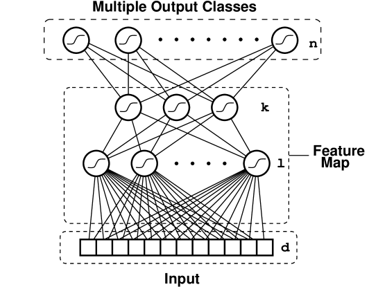
Figure 2: Neural network for feature learning. The feature map is implemented by the first two hidden layers. The $n$ output nodes correspond to the $n$ different tasks in the $(n,m)$-sample $\bf z$.

In general, a set of features may be viewed as a map from the (typically high-dimensional) input space ${R}^{d}$ to a much smaller dimensional space ${R}^{k}$ ($k\ll d$). Any such bounded feature map can be approximated to arbitrarily high accuracy by a one-hidden-layer neural network with $k$ output nodes. This is illustrated in Figure 2. Fixing the number of nodes in the first hidden layer, let $\Phi_{w}\colon{R}^{d}\to{R}^{k}$ denote the feature map computed by the the neural network with weights $w$. The set of all such feature maps is $\{\Phi_{w}\colon w\in{R}^{W}\}$ where $W$ is the number of weights in the first two layers.

For argument’s sake, assume the “simple functions” of the features (mentioned in the above quote) are squashed linear maps. Denoting the $k$ components of the feature map $\Phi_{w}$ by $\phi_{w,1},\dots,\phi_{w,k}$, each setting of the feature map weights generates a hypothesis space ${\cal H}_{w}$ by

$${\cal H}_{w}:=\left\{\sigma\left(\sum_{i=1}^{k}\alpha_{i}\phi_{w,i}\right)\colon(\alpha_{1},\dots,\alpha_{k})\in{R}^{k}\right\},$$ (36)

where $\sigma\colon{R}\to{R}$ is the squashing function. ${\cal H}_{w}$ is simply the set of all squashed linear functions of the features $\Phi_{w}$. The set of all such hypothesis spaces,

$${\mbox{\boldmath$\bf H$}}:=\{{\cal H}_{w}\colon w\in{R}^{W}\}$$ (37)

is a hypothesis space family.

Finding the right set of features for the environment $({\cal P},Q)$ is equivalent to finding the right hypothesis space ${\cal H}_{w}\in{\mbox{\boldmath$\bf H$}}$.

As in the previous section, the correct set of features may be learnt by finding a hypothesis space with small error on a sufficiently large $(n,m)$-sample $\bf z$ (recall that an $(n,m)$-sample is simply $n$ training sets corresponding to $n$ different learning tasks). Specializing to squared loss, in the present framework the error of ${\cal H}_{w}$ on $\bf z$ (equation (3)) is given by

$${\hat{{\mbox{er}}}}_{\mbox{\boldmath$\bf z$}}({\cal H}_{w})=\frac{1}{n}\sum_{i=1}^{n}\inf_{(\alpha_{1},\dots,\alpha_{k})\in{R}^{k}}\frac{1}{m}\sum_{j=1}^{m}\left[\sigma\left(\sum_{l=1}^{k}\alpha_{l}\phi_{w,l}(x_{ij})\right)-y_{ij}\right]^{2}$$ (38)

Using gradient descent and an $n$ output node network as in figure 2, output weights $(\alpha_{1},\dots,\alpha_{k})$ and feature weights $w$ minimizing (38) can be found. For details see [4].

The size of $\bf z$ ensuring that the resulting features will be good for learning novel tasks from the same environment is given by theorem 2. All we have to do is compute the logarithm of the covering numbers ${\cal C}({\varepsilon},{\mbox{\boldmath$\bf H$}}^{n}_{l})$ and ${\cal C}({\varepsilon},{\mbox{\boldmath$\bf H$}}^{*})$. If the feature weights $w$ and the output weights $\alpha_{1},\dots,\alpha_{k}$ are bounded, and the squashing function $\sigma$ is Lipschitz, then there exist constants $\kappa,\kappa^{\prime}$ (independent of ${\varepsilon},W$ and $k$) such that for all ${\varepsilon}>0$,

$$\ln{\cal C}({\varepsilon},{\mbox{\boldmath$\bf H$}}^{n}_{l}) \leq 2\left(kn+W\right)\ln\frac{\kappa}{{\varepsilon}}$$

$$\ln{\cal C}({\varepsilon},{\mbox{\boldmath$\bf H$}}^{*}) \leq 2W\ln\frac{\kappa^{\prime}}{{\varepsilon}}$$

(see [5] for a proof). Plugging these expressions into theorem 2 gives the following theorem.

Theorem 4

Let ${\mbox{\boldmath$\bf H$}}=\{{\cal H}_{w}\}$ be a hypothesis space family where each hypothesis space ${\cal H}_{w}$ is a set of squashed linear maps composed with a neural network feature map, as above. Suppose the number of features is $k$, and the total number of feature weights is W. Assume all feature weights and output weights are bounded, and the squashing function $\sigma$ is Lipschitz. Let $\bf z$ be an $(n,m)$-sample generated from the environment $({\cal P},Q)$. If

$$n\geq O\left(\frac{1}{{\varepsilon}^{2}}\left[W+\log\frac{1}{\delta}\right]\right),$$ (39)

and

$$m\geq O\left(\frac{1}{{\varepsilon}^{2}}\left[k+\frac{1}{n}\left(W+\log\frac{1}{\delta}\right)\right]\right)$$ (40)

then with probability at least $1-\delta$ any ${\cal H}_{w}$ will satisfy

$${\mbox{er}}_{Q}({\cal H}_{w})\leq{\mbox{er}}_{\mbox{\boldmath$\bf z$}}({\cal H}_{w})+{\varepsilon}.$$ (41)

Notes:

1. Keeping the accuracy paramters ${\varepsilon}$ and $\delta$ fixed, the upper bound on the number of examples required of each task behaves like $O(k+W/n)$. The same upper bound also applies in theorem 3.

2. Once the feature map is learnt, only the output weights have to be estimated to learn a novel task. Again keeping the accuracy parameters fixed, this requires no more that $O(k)$ examples.

3. Thus, as the number of tasks learnt increseas, the upper bound on the number of examples required of each task decays to the minimum possible, $O(k)$.

4. If the “small number of strong features” assumption is correct, then $k$ will be small. However, typically we will have very little idea of what the features are, so the size of the feature network will have to be huge, so $W\gg k$.

5. $O(k+W/n)$ decreases most rapidly with increasing $n$ when $W\gg k$, so at least in terms of the upper bound on the number of examples required per task, learning small feature sets is an ideal application for learning to learn.

6. Note that if we do away with the feature map altogether then $W=0$ and the upper bound on $m$ becomes $O(k)$, independent of $n$. So in terms of the upper bound, learning $n$ tasks becomes just as hard as learning one task. At the other extreme, if we fix the output weights then effctively $k=0$ and the number of examples required of each task decreases as $O(W/n)$. Thus a range of behaviour in the number of examples required of each task is possible: from no improvement at all to an $O(1/n)$ decrease as the number of tasks $n$ increases.

7. To rigorously conclude that learning $n$ tasks is better than learning one, we would have to show a matching lower bound of $\Omega(k+W/n)$ on the number of examples required of each task. Rather than search for lower bounds within the EP model (which are difficult to prove), we discuss a Bayes model of learning to learn in the next section where simultaneous upper and lower bounds appear more naturally.

4 The Bayes model of learning to learn

Recall from section 2.2 that in Bayesian models of ordinary learning the learner’s bias is represented by the space of possible distributions $\{P_{\theta}\colon\theta\in\Theta\}$ along with the choice of prior $p(\theta)$. The learning task $P$ is assumed to be equal to some $P_{\theta^{*}}$ where $\theta^{*}\in\Theta$.

Observe that $p(\theta)$ is a subjective prior distribution over a set of distributions $\{P_{\theta}\}$. It is subjective because it simply reflects the prior beliefs of the learner, not some objective stochastic phenomenon. Now note that the environment $({\cal P},Q)$ consists of a set of distributions ${\cal P}$, and a distribution $Q$ on ${\cal P}$, and furthermore that ${\cal P}$ can be sampled according to $Q$ to generate multiple tasks $P_{1},\dots,P_{n}$ (recall the discussion in section 3). This makes $Q$ an objective prior distribution. Objective in the sense that it can be sampled, i.e. it corresponds to some objective stochastic phenomenon.

If we assume ${\cal P}=\{P_{\theta}\colon\theta\in\Theta\}$ (so now ${\cal P}$ is a restricted subset of all possible distributions on $X\times Y$), the goal of a bias learner in this framework is to find the right prior distribution $Q$. To do this, the learner must have available a set of possible prior distributions $\{P_{\pi}\colon\pi\in\Pi\}$ from which to choose. Each $P_{\pi}$ is a distribution on $\Theta$. We assume realizability, so that $Q=P_{\pi^{*}}$ for some $\pi^{*}\in\Pi$.

To summarize, the Bayes model of learning to learn consists of the following ingredients:

• An input space $X$ and an output space $Y$,

• a set of probability distributions $P_{\theta}$ on $X\times Y$, parameterised by $\theta\in\Theta$,

• a set of prior distributions $P_{\pi}$ on $\Theta$, parameterised by $\pi\in\Pi$.

• an objective or environmental prior distribution $P_{\pi^{*}}$ where $\pi^{*}\in\Pi$.

• To complete the model, the learner also has a subjective hyper-prior distribution $P_{\Pi}$ on $\Pi$.

The two-tiered structure with a set of possible priors $\{P_{\pi}\colon\pi\in\Pi\}$ and a hyper-prior $p(\pi)$ on $\Pi$ makes this model an example of a hierarchical Bayesian model [7, 9].

As with the EP model, the learner receives an $(n,m)$-sample $\bf z$, generated by first sampling $n$ times from $\Theta$ according $P_{\pi^{*}}$ to give $\theta_{1},\dots,\theta_{n}$, and then sampling $m$ times from each $X\times Y$ according to each $P_{\theta_{i}}$ to generate $z_{i}=(x_{i1},y_{i1}),\dots,(x_{im},y_{im})$. To simplify the notation in this section, let $Z:=X\times Y$ and $z_{ij}:=(x_{ij},y_{ij})$. As it will be necessary to distinguish between $(n,m-1)$ samples and $(n,m)$ samples, this will be made explicit in the notation by writing ${z^{(n,m)}}$ instead of $\bf z$:

$${z^{(n,m)}}=\begin{array}[]{ccc}z_{11}&\cdots&z_{1m}\\ \vdots&\ddots&\vdots\\ z_{n1}&\cdots&z_{nm}\end{array}$$ (42)

4.1 Loss as the extra information required to predict the next observation

Recall that in the Bayes model of single task learning (section 2.2), the learner’s loss was measured by the amount of extra information needed to encode novel examples of the task. So one way to measure the advantage in learning $n$ tasks together is by the rate at which the learner’s loss in predicting novel examples decays for each task. This question is similar to that addressed by theorem 3.

So fix the number of tasks $n$, sample $n$ tasks $\theta^{n}=\theta_{1},\dots,\theta_{n}$ according to the true prior $P_{\pi^{*}}$, and then for each $m=1,2,\dots$ the learner has already seen $m-1$ examples of each task:

$${z^{(n,m-1)}}=\begin{array}[]{ccc}z_{11}&\cdots&z_{1m-1}\\ \vdots&\ddots&\vdots\\ z_{n1}&\cdots&z_{nm-1}\end{array}$$ (43)

where each row is drawn according to $P^{m-1}_{\theta_{i}}$ (or equivalently, each column is drawn according to $P_{\theta^{n}}$). The learner then:

• generates the posterior distribution $p(\theta^{n}|{z^{(n,m-1)}})$ on the set of all $n$ tasks, $\Theta^{n}$, according to Bayes’ rule:

  $$p(\theta^{n}|{z^{(n,m-1)}}) = \frac{p({z^{(n,m-1)}}|\theta^{n})p(\theta^{n})}{p({z^{(n,m-1)}})}$$ (44)

  $$= \frac{p(\theta^{n})\prod_{i=1}^{n}\prod_{j=1}^{m-1}p(z_{ij}|\theta_{i})}{p({z^{(n,m-1)}})}$$

  where $p({z^{(n,m-1)}})=\int_{\Theta^{n}}p(\theta^{n})\prod_{i=1}^{n}\prod_{j=1}^{m-1}p(z_{ij}|\theta_{i})\,d\theta^{n}$.

• uses the posterior distribution to generate a predictive distribution on $Z^{n}$,

  $$p(z^{n}|{z^{(n,m-1)}})=\int_{\Theta^{n}}p(z^{n}|\theta^{n})p(\theta^{n}|{z^{(n,m-1)}})\,d\theta^{n},$$ (45)

• and suffers a loss, ${\overline{L}}_{n,m}$, equal to the expected amount of extra information needed per task to encode a novel example of each task using the predictive distribution $p(z^{n}|{z^{(n,m-1)}})$, over and above the minimum amount of information, i.e. the information required using the true distribution, $p(z^{n}|\theta^{n})$:

  $${\overline{L}}_{n,m}:=\frac{1}{n}E_{{Z^{n}}|\theta^{n}}\log\frac{p(z^{n}|\theta^{n})}{p(z^{n}|{z^{(n,m-1)}})}.$$ (46)

Note that the loss at the first trial is:

$${\overline{L}}_{n,1}:=E_{{Z^{n}}|\theta^{n}}\log\frac{p(z^{n}|\theta^{n})}{p(z^{n})},$$ (47)

where $p(z^{n})$ is the learner’s initial distribution on ${Z^{n}}$ before any data has arrived,

$$p(z^{n})=\int_{\Theta^{n}}p(z^{n}|\theta^{n})p(\theta^{n})\,d\theta^{n}=\int_{\Pi}\int_{\Theta^{n}}p(z^{n}|\theta^{n})p(\theta^{n}|\pi)\,d\theta^{n}\,p(\pi)\,d\pi$$ (48)

To understand better the meaning of ${\overline{L}}_{n,m}$, consider the loss associated with learning a single classification task. In this case $Z=X\times\{0,1\}$. If we assume that only the conditional distribution on class labels is affected by the model, then $p(z|\theta)=p(x)p(y|x,\theta)$, and for the predictive distribution, $p(z|z^{m})=p(x)p(y|x,z^{m})$. Let $\alpha(x):=p(y=1|x,\theta)$ and $\beta(x):=p(y=1|x,z^{m})$. Substituting these expressions into (46) and simplifying yields

$${\overline{L}}_{1,m}=E_{X}\left[\alpha(x)\log\frac{\alpha(x)}{\beta(x)}+(1-\alpha(x))\log\frac{1-\alpha(x)}{1-\beta(x)}\right].$$ (49)

The expression in square brackets is zero if $\alpha(x)=\beta(x)$, i.e. if the conditional distributions on class labels are the same for the true and predictive distributions. It increases slowly as $\alpha(x)$ and $\beta(x)$ diverge.

It turns out that ${\overline{L}}_{n,m}$ is difficult to analyse, so instead we look at the cumulative loss over a sequence of trials:

$${\overline{C}}_{n,m,\pi^{*}}:=\sum_{k=0}^{m-1}E_{\Theta^{n}|\pi^{*}}E_{Z^{(n,k)}|\theta^{n}}{\overline{L}}_{n,k+1},$$ (50)

i.e. the expected total loss incurred by the learner after $m$ steps of the above process. Note that the expectation is over all sequences of $n$ tasks $\theta^{n}$ drawn according to $P_{\pi^{*}}$ and all $(n,k)$-samples drawn according to $p(z^{n}|\theta^{n})$.

4.2 $\bf(a,b)$ models

In [6], the asymptotic behaviour of ${\overline{C}}_{n,m,\pi^{*}}$ as a function of $m$ was analysed for general hierarchical models. To illustrate the results, and to show how they apply to the feature learning example of section 3.2, here we will restrict our attention to $(a,b)$-models. The concept of an $(a,b)$-model was formally defined in [6] as follows:

Definition 5

An $(a,b)$-model is a hierarchical model in which $\Pi={R}^{b}$, $\Theta={R}^{a}\times{R}^{b}$ and the following conditions hold:

1. The priors $p(\theta|\pi)$ are of the form

   $$p(\theta=(x^{a},x^{b})|\pi)=\delta(x^{b}-\pi)g_{\pi}(x_{a})$$ (51)

   where $\delta(\cdot)$ is the $b$-dimensional Dirac delta function and $g_{\pi}$ is a continuous function on ${R}^{a}$ that also varies continuously with $\pi$.

2. The hyper-prior on $\Pi$, $P_{\Pi}$ has continuous density $p(\pi)$ and the true prior $\pi^{*}$ has positive density $p(\pi^{*})$.

3. The conditional distributions $p(z|\theta)$ are twice continuously differentiable functions of $\theta$.

The definition of an $(a,b)$-model in [6] contains two technical conditions which have been omitted in the above definition. The interested reader is referred to that paper for a full discussion. Condition 1 of an $(a,b)$-model formalizes the idea of a hierarchical model in which there are $a+b$ parameters, $b$ of which are effectively hyper-parameters and are fixed by the prior and the remaining $a$ of which are model parameters. Conditions 2 and 3 ensure realizability and an appropriate level of smoothness.

The following definition is needed to state the main theorem.

Definition 6

Let $(X,\Sigma,P)$ be a measure space and $f,g\colon N\times X\to{R}$ ($N$ is the positive integeres) be two real-valued functions on $N\times X$ such that for all $n\in N$, $f(n,\cdot)$ and $g(n,\cdot)$ are measurable functions on $X$. Set $X_{n}:=\{x\colon f(n,x)=g(n,x)\}$ for each $n\in N$. We say

$$f(n,x)\doteq_{(X,P)}g(n,x)$$ (52)

if $\lim_{n\rightarrow\infty}P(X_{n})=1$. This will be abbreviated to $f(n,x)\doteq g(n,x)$ when $X$ and $P$ are clear from the context.

For the following theorem, fix $n$ and take all limiting behaviour with respect to $m$.

Theorem 5 ([6],Theorem 6)

In an $(a,b)$-model, the learner’s cumulative risk (50) satisfies

$${\overline{C}}_{n,m,\pi^{*}}\doteq_{\Pi,P_{\Pi}}\frac{\log m}{2}\left(a+\frac{b}{n}\right)+o\left(\log m\right).$$ (53)

If the true prior $\pi^{*}$ is known then

$${\overline{C}}_{n,m,\pi^{*}}=\frac{\log m}{2}\left(a\right)+o\left(\log m\right).$$ (54)

Note that equation (54) is an equality. In [6] it was stated as a $\doteq$ relation but in fact the stronger expression holds.

Comparing (53) and (54), we see that as the number of tasks $n$ increases, the effect of lack of knowledge of the true prior can be made arbitrarily small. Also, learning multiple tasks is most advantageous when $b\gg a$, i.e. when the true model is quite small but our uncertainty concerning the true model is large. This is a similar conclusion to the one reached in section 3.2 (see note 3 after theorem 3.

4.3 Learning features within the Bayes model

Consider the feature learning model of section 3.2 (recall figure 2). In this case, $\Theta$ is the set of all possible neural networks implementable by fixing the feature weights and the weights of a single output node. As there are $k$ output weights and $W$ feature weights, $\Theta={R}^{k+W}$. The realizability assumption means there exists a fixed set of features such that all tasks in the environment can be implemented by composing a squashed linear map with the feature set. Thus, the true prior distribution $p(\theta|\pi^{*})$ is a delta-function over the correct feature weight setting, combined with an appropriate distribution over the $k$ output weights (one that generates the tasks in the environment with the correct frequency). Assuming the output-weight distribution is continuous, the true prior is of the form (51), with $a=k$ and $b=W$. The set of all such priors is simply the set of all distributions that are a delta function over some feature weight setting, combined with a continuous distribution over the output weights. To complete the model, suppose that for each $\theta\in{R}^{k+W}$, $p(z|\theta)$ is of the form

$$p(y=1,x|\theta) = p(x)f_{\theta}(x)$$

$$p(y=0,x|\theta) = p(x)(1-f_{\theta}(x))$$

where $f_{\theta}(x)$ is the output of the network with weights $\theta$ and input $x$, and $p(x)$ is a continuous density on some compact subset of ${R}^{d}$. Assume the sigmoid on the hidden nodes is $\sigma(x)=\tanh(x)$, and on the output node is $\sigma(x)=(1+\tanh(x))/2$.

With these assumptions, the neural network feature learning model is a $(k,W)$-model in the sense of definition 5. Unfortunately, the neural network feature model does not satisfy the technical conditions mentioned after definition 5, so a straightforward application of theorem 5 is not possible. However, the difficulties are not insurmountable (see [6] for the details) and so we obtain the following theorem:

Theorem 6

For the neural-network feature learning model as above, the cumulative risk (50) satisfies

$${\overline{C}}_{n,m,\pi^{*}}\doteq\frac{\log m}{2}\left(k+\frac{W}{n}\right)+o\left(\log m\right).$$ (55)

If the true prior is known (i.e. the true feature weights are known), then

$${\overline{C}}_{n,m,\pi^{*}}=\frac{\log m}{2}\left(k\right)+o\left(\log m\right).$$ (56)

Note the reappearance of the factor $k+W/n$ (recall theorem 3 and the notes afterwards). Comparing equations (55) and (56) we see again that the effect of ignorance of the true prior (in this case ignorance of the right features) can be made arbitrarily small by learning sufficiently many tasks. The improvement is greatest when the number of features ($k$) is small, but our uncertainty as to what the right feature set should be is large.

5 Conclusion

Two mathematical models of bias learning (or learning to learn) have been discussed: one based on Empirical process theory and the other a Hierarchical Bayesian model. Both models show that if a learning machine is embedded within an environment of related learning tasks, then it can learn its own bias for the environment by learning sufficiently many tasks. Bounds were given on the number of tasks and number of examples of each task needed to ensure good generalisation from a bias learner. Good generalisation in this case means that with high probability the learner’s choice of hypothesis space will contain good solutions to novel tasks drawn from the same environment. The theory was specialised to the case of feature learning with neural networks.

There are many pattern classification problems that can be viewed as consisting of large number of related tasks and that seem to possess small feature sets. Speech recognition, character recognition, face recognition and fingerprint recognition all fit this bill. Feature learning in these domains should be particularly successful.

References

- [1] Martin Anthony and Norman Biggs. Computational Learning Theory. Cambridge University Press, Cambridge, 1992.
- [2] Andrew Barron and Bertrand Clarke. Jeffreys’ Prior is Asymptotically Least Favourable under Entropy Risk. Journal of Statistical Planning and Inference, 41:37–60, 1994.
- [3] Jonathan Baxter. A Model of Bias Learning. Technical Report LSE-MPS-97, London School of Economics, Centre for Discrete and Applicable Mathematics, November 1995. Submitted for publication. Copy available from http://keating.anu.edu.au/jon/papers/lse.ps.gz.
- [4] Jonathan Baxter. Learning Internal Representations. In Proceedings of the Eighth International Conference on Computational Learning Theory, pages 311–320. ACM Press, 1995.
- [5] Jonathan Baxter. Learning Internal Representations. PhD thesis, Department of Mathematics and Statistics, The Flinders University of South Australia, 1995. Copy available from http://keating.anu.edu.au/jon/papers/thesis.ps.gz.
- [6] Jonathan Baxter. A Bayesian/Information Theoretic Model of Learning to Learn via Multiple Task Sampling. Machine Learning, 1997. To Appear.
- [7] James O Berger. Multivariate Estimation: Bayes, Empirical Bayes, and Stein Approaches. SIAM, 1986.
- [8] Bertrand Clarke and Andrew Barron. Information-Theoretic Asymptotics of Bayes Methods. IEEE Transactions on Information Theory, 36:453–471, 1990.
- [9] I J Good. Some History of the Hierarchical Bayesian Methodology. In J M Bernado, M H De Groot, D V Lindley, and A F M Smith, editors, Bayesian Statistics II. University Press, Valencia, 1980.
- [10] David Hume. A Treatise of Human Nature. 1737.
- [11] Tom M Mitchell. The need for biases in learning generalisations. In Tom G Dietterich and Jude Shavlik, editors, Readings in Machine Learning. Morgan Kaufmann, 1991.
- [12] V N Vapnik. Estimation of Dependences based on Empirical Data. Springer-Verlag, New York, 1982.
- [13] V N Vapnik and A Ya Chervonenkis. On the uniform convergence of relative frequencies of events to their probabilities. Theory Probab. Appl., 16:264–280, 1971.