Sub-Goal Trees – a Framework for Goal-Based Reinforcement Learning

Abstract

Many AI problems, in robotics and other domains, are goal-based, essentially seeking trajectories leading to various goal states. Reinforcement learning (RL), building on Bellman’s optimality equation, naturally optimizes for a single goal, yet can be made multi-goal by augmenting the state with the goal. Instead, we propose a new RL framework, derived from a dynamic programming equation for the all pairs shortest path (APSP) problem, which naturally solves multi-goal queries. We show that this approach has computational benefits for both standard and approximate dynamic programming. Interestingly, our formulation prescribes a novel protocol for computing a trajectory: instead of predicting the next state given its predecessor, as in standard RL, a goal-conditioned trajectory is constructed by first predicting an intermediate state between start and goal, partitioning the trajectory into two. Then, recursively, predicting intermediate points on each sub-segment, until a complete trajectory is obtained. We call this trajectory structure a sub-goal tree. Building on it, we additionally extend the policy gradient methodology to recursively predict sub-goals, resulting in novel goal-based algorithms. Finally, we apply our method to neural motion planning, where we demonstrate significant improvements compared to standard RL on navigating a 7-DoF robot arm between obstacles.

1 Introduction

Many AI problems can be characterized as learning or optimizing goal-based trajectories of a dynamical system, for example, robot skill learning and motion planning (Mülling et al., 2013; Gu et al., 2017; LaValle, 2006; Qureshi et al., 2018). The reinforcement learning (RL) formulation, a popular framework for trajectory optimization based on Bellman’s dynamic programming (DP) equation (Bertsekas & Tsitsiklis, 1996), naturally addresses the case of a single goal, as specified by a single reward function. RL formulations for multiple goals have been proposed (Schaul et al., 2015; Andrychowicz et al., 2017), typically by augmenting the state space to include the goal as part of the state, but without changing the underlying DP structure.

On the other hand, in deterministic shortest path problems, multi-goal trajectory optimization is most naturally represented by the all-pairs shortest path (APSP) problem (Russell & Norvig, 2010). In this formulation, augmenting the state and using Bellman’s equation is known to be sub-optimal, and dedicated APSP algorithms such as Floyd-Warshall (Floyd, 1962) build on different DP principles. Motivated by this, we propose a goal-based RL framework that builds on an efficient APSP solution, and is also applicable to large or continuous state spaces using function approximation.

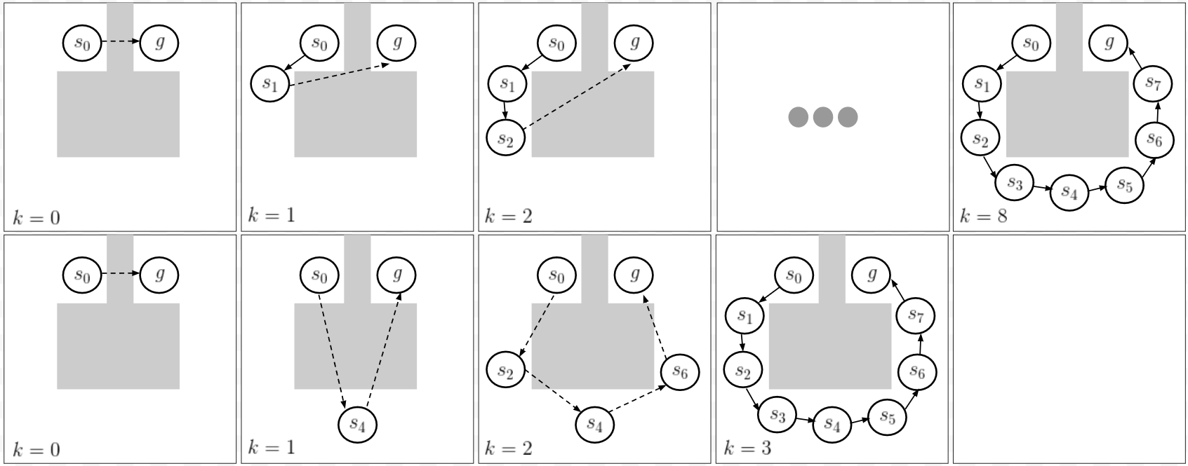
Figure 1: Trajectory prediction methods. Upper row: a conventional Sequential representation. Lower row: Sub-Goal Tree representation. Solid arrows indicate predicted segments, while dashed arrows indicate segments that still require to be predicted. By concurrently predicting sub-goals, a Sub-Goal Tree only requires $3$ sequential computations, while the sequential requires $8$.

Our key idea is that a goal-based trajectory can be constructed in a divide-and-conquer fashion. First, predict a sub-goal between start and goal, partitioning the trajectory into two. Then, recursively, predict intermediate sub-goals on each sub-segment, until a complete trajectory is obtained. We call this trajectory structure a sub-goal tree (Figure 1), and we develop a DP equation for APSP that builds on it and is compatible with function approximation. We further bound the error of following the sub-goal tree trajectory in the presence of approximation errors, and show favorable results compared to the conventional RL method, intuitively, due to the sub-goal tree’s lower sensitivity to drift.

The sub-goal tree can also be seen as a general parametric structure for a trajectory, where a parametric model, e.g., a neural network, is used to predict each sub-goal given its predecessors. Based on this view, we develop a policy gradient framework for sub-goal trees, and show that conventional policy-gradient techniques such as control variates and trust regions (Greensmith et al., 2004; Schulman et al., 2015) naturally apply here as well.

Finally, we present an application of our approach to neural motion planning – learning to navigate a robot between obstacles (Qureshi et al., 2018; Jurgenson & Tamar, 2019). Using our policy gradient approach, we demonstrate navigating a 7-DoF continuous robot arm safely between obstacles, obtaining marked improvement in performance compared to conventional RL approaches.

2 Related work

In RL, the idea of sub-goals has mainly been investigated under the options framework (Sutton et al., 1999). In this setting, the goal is typically fixed (i.e., given by the reward in the MDP), and useful options are discovered using some heuristic such as bottleneck states (McGovern & Barto, 2001; Menache et al., 2002) or changes in the value function (Konidaris et al., 2012). While hierarchical RL using options seems intuitive, theoretical results for their advantage are notoriously difficult to establish, and current results require non-trivial assumptions on the option structure (Mann & Mannor, 2014; Fruit et al., 2017). Interestingly, by investigating the APSP setting, we obtain general and strong results for the advantage of sub-goals.

Universal value functions (Schaul et al., 2015; Andrychowicz et al., 2017) learn a goal-conditioned value function using the Bellman equation. In contrast, in this work we propose a principled motivation for sub-goals based on the APSP problem, and develop a new RL formulation based on this principle. A connection between RL and the APSP has been suggested by Kaelbling (1993); Dhiman et al. (2018), based on the Floyd-Warshall algorithm. However, as discussed in Section 4.2, these approaches become unstable once function approximation is introduced. Goal-conditioned policies are also related to universal plans in the classical planning literature (Schoppers, 1989; Kaelbling, 1988; Ginsberg, 1989), and in this sense SGTs can be used to approximate universal plans using learning.

Sub-goal trees can be seen as a form of trajectory representation (as we discuss in Section 5.2). Such has been investigated for learning robotic skills (Mülling et al., 2013; Sung et al., 2018) and navigation (Qureshi et al., 2018). A popular approach, dynamical movement primitives  (Ijspeert et al., 2013), represents a continuous trajectory as a dynamical system with an attractor at the goal, and was successfully used for RL (Kober et al., 2013; Mülling et al., 2013; Peters & Schaal, 2008). The temporal segment approach of Mishra et al. (2017), on the other hand, predicts segments of a trajectory sequentially. In the context of video prediction, Jayaraman et al. (2019) proposed to predict salient frames in a goal-conditioned setting by a supervised learning loss that focuses on the ‘best’ frames. This was used to predict a list of sub-goals for a tracking controller. In contrast, we investigate the RL problem, and predict sub-goals recursively.

Approximate APSP solutions have been traditionally explored in the non-learning setting. Approaches such as in Thorup & Zwick (2005); Chan (2010); Williams (2014) compute $k$-optimal paths ($k>1$) in running time that is sub-cubic in the number of vertices in the graph. These methods require full knowledge of the graph and process each vertex at least once. In contrast, our learning-based approach can generalize to unseen states (vertices) by learning from similar states, potentially scaling to very large or even continuous state spaces, as we demonstrate in our experiments.

3 Problem Formulation and Notation

We are interested in optimizing goal-conditioned tasks in dynamical systems. We restrict ourselves to deterministic, stationary, and finite time systems, and consider both discrete and continuous state formulations.

In the discrete state setting, we study the all-pairs shortest path (APSP) problem on a graph. Consider a directed and weighted graph with $N$ nodes $s_{1},\dots,s_{N}$, and denote by $c(s,s^{\prime})\geq 0$ the weight of edge $s\to s^{\prime}$. By definition, we set $c(s,s)=0$, such that the shortest path from a node to itself is zero. To simplify notation, we can replace unconnected edges by edges with weight $\infty$. Thus, without loss of generality, throughout this work we assume that the graph is complete. The APSP problem seeks the shortest paths (i.e., a path with minimum sum of costs) from any start node $s$ to any goal node $g$ in the graph:

$$\min_{T,s_{0}=s,s_{1},\dots,s_{T-1},s_{T}=g}\sum_{t=0}^{T-1}c(s_{t},s_{t+1}).$$ (1)

In the continuous state case, we consider a deterministic controlled dynamical system in discrete time, defined over a state space $S$ and an action space $U$: where $s_{t},s_{t+1}\in S$ are the states at time $t$ and $t+1$, respectively, $u_{t}\in U$ is the control at time $t$, and $f$ is a stationary state transition function. Given an initial state $s_{0}$ and a goal $g$, an optimal trajectory reaches $g$ while minimizing the sum of non-negative costs $\bar{c}(s,u)\geq 0$:

$$\min_{T,u_{0},\dots,u_{T}}\sum_{t=0}^{T}\bar{c}(s_{t},u_{t}),\textrm{ s.t. }{s_{t+1}}\!=\!{f}({s_{t}},{u_{t}}),{s_{T}}\!=\!g.$$ (2)

To unify our treatment of problems (1) and (2), in the remainder of this paper we abstract away the actions as follows. Let $c(s,s^{\prime})=\min_{u}\bar{c}(s,u)\textrm{ s.t. }{s^{\prime}}={f}({s},{u})$, and $c(s,s^{\prime})=\infty$ if no transition from $s$ to $s^{\prime}$ is possible. Then, for any start and goal states $s,g$, Eq. (2) is equivalent to:

$$\min_{T,s_{0}=s,s_{1},\dots,s_{T-1},s_{T}=g}\sum_{t=0}^{T-1}c(s_{t},s_{t+1}).$$ (3)

Note the similarity of Problem (3) to the APSP problem (1), where feasible transitions of the dynamical system are represented by edges between states in the graph. In the rest of this paper, we study solutions for (1) and (3), for all start and goal pairs $s,g$. We are particularly interested in large problems, where exact solutions are intractable, and approximations are required.

Notation: Let $\tau\!=\!s_{0},\dots,s_{T}$ denote a state trajectory. Also, denote $c_{i:j}\!=\!\sum_{t=i}^{j-1}{\!c(s_{t},s_{t+1})}$, the cost of several subsequent states and $c_{\tau}=c_{0:T}$ as the total trajectory cost. Let $\tau(s_{0},s_{m})\!\!=\!\!s_{0},\dots,s_{m}$ denote the segment of $\tau$ starting at $s_{0}$ and ending at $s_{m}$. We denote the trajectory concatenation as $\tau\!\!=\!\![\tau(s_{0},s_{m}),\tau(s_{m},s_{T})]$, where it is implied that $s_{m}$ appears only once. For a stochastic trajectory distribution conditioned on start and goal, we denote $\Pr_{\pi}[s_{i},\dots,s_{j}|s,g]$ as shorthand for $\Pr_{\pi}[s_{i},\dots,s_{j}|s_{i}\!=\!s,\!s_{j}\!=\!g]$.

4 Approximate Dynamic Programming

In this section we study a dynamic programming principle for the APSP problem (1). We will later extend our solution to the continuous case (3) using function approximation.

One way to solve (1) is to solve a single-goal problem for every possible goal state. The RL equivalent of this approach is UVFA, suggested by Schaul et al. (2015), where the state space is augmented with the goal state, and a goal-based value function is introduced. The UVFA is optimized using standard (single-goal) RL, by learning over different goals. Alternatively, our approach builds on an efficient APSP dynamic programming algorithm, as we propose next.

4.1 Sub-Goal Tree Dynamic Programming

By our definition of non-negative costs, the shortest path between any two states is of length at most $N$. The main idea in our approach is that a trajectory between $s$ and $g$ can be constructed in a divide-and-conquer fashion: first predict a sub-goal between start and goal that optimally partitions the trajectory to two segments of length $N/2$ or less: $s,\dots,s_{N/2}$ and $s_{N/2},\dots,g$. Then, recursively, predict intermediate sub-goals on each sub-segment, until a complete trajectory is obtained. We term this composition a sub-goal tree (SGT), and we formalize it as follows.

Let $V_{k}(s,s^{\prime})$ denote the shortest path from $s$ to $s^{\prime}$ in $2^{k}$ steps or less. Note that by our convention about unconnected edges above, if there is no such trajectory in the graph then $V_{k}(s,s^{\prime})=\infty$. We observe that $V_{k}$ obeys the following dynamic programming relation, which we term sub-goal tree dynamic programming (SGTDP).

Theorem 1.

Consider a weighted graph with $N$ nodes and no negative cycles. Let $V_{k}(s,s^{\prime})$ denote the cost of the shortest path from $s$ to $s^{\prime}$ in $2^{k}$ steps or less, and let $V^{*}(s,s^{\prime})$ denote the cost of the shortest path from $s$ to $s^{\prime}$. Then, $V_{k}$ can be computed according to the following equations:

$$\begin{split}V_{0}(s,s^{\prime})&=c(s,s^{\prime}),\quad\forall s,s^{\prime}:s\neq s^{\prime};\\ V_{k}(s,s)\text{ }&=0,\quad\forall s;\\ V_{k}(s,s^{\prime})&=\!\min_{s_{m}}\!\left\{V_{k-1}(s,s_{m})\!+\!V_{k-1}(s_{m},s^{\prime})\right\}\!,\forall s,\!s^{\prime}\!\!:\!s\!\neq\!s^{\prime}\!.\end{split}$$ (4)

Furthermore, for $k\geq\log_{2}(N)$ we have that $V_{k}(s,s^{\prime})=V^{*}(s,s^{\prime})$ for all $s,s^{\prime}$.

The proof of Theorem 1, along with all other proofs in this paper, is reported in the supplementary material.

Given $V_{0},\dots,V_{\log_{2}(N)}$, Theorem 1 prescribes the following recipe for computing a shortest path for every $s,g$, which we term the greedy SGT trajectory:

$$s_{0} =s,\text{ }s_{N}=g$$ (5)

$$s_{N/2} \in\operatorname*{arg\,min}_{s_{m}}\!\left\{\!V_{\log_{2}(N)-1}(\!s_{0},s_{m}\!)\!+\!V_{\log_{2}(N)-1}(s_{m},s_{N})\!\right\}\!,$$

$$s_{N/4} \in\operatorname*{arg\,min}_{s_{m}}\!\left\{\!V_{\log_{2}(N)-2}(\!s_{0},s_{m}\!)\!+\!V_{\log_{2}(N)-2}(s_{m},s_{N/2})\!\right\}\!,$$

$$s_{3N/4} \in\operatorname*{arg\,min}_{s_{m}}\!\left\{\!V_{\log_{2}(N)-2}(\!s_{N/2},s_{m}\!)\!+\!V_{\log_{2}(N)-2}(s_{m},s_{N})\!\right\}\!,$$

$$\dots$$

The SGT can be seen as a general divide-and-conquer representation of a trajectory, by recursively predicting sub-goals. In contrast, the construction of a greedy trajectory in conventional RL (using the Bellman equation) proceeds sequentially, by predicting state (or action) after state. This is illustrated in Figure 1. We next investigate the advantages of the SGT structure compared to the sequential approach.

In conventional RL, it is well known that in the presence of errors, following a greedy policy may suffer from drift – accumulating errors that may hinder performance (Ross et al., 2011). In the goal-based setting, intuitively, the error magnitude scales with the distance from the goal. Our main observation is that the SGT is less sensitive to drift, as the sub-goals break the trajectory into smaller segments with exponentially decreasing errors. We next formalize this idea, by analyzing an approximate DP formulation.

4.2 SGT Approximate DP

Similar to standard dynamic programming algorithms, the SGTDP algorithm iterates over all states in the graph, which becomes infeasible for large, or continuous state spaces. For such cases, inspired by the approximate dynamic programming (ADP) literature (Bertsekas, 2005), we investigate ADP methods based on SGTDP.

Let $T$ denote the SGTDP operator, $(TV)(s,s^{\prime})=\min_{s_{m}}\left\{V(s,s_{m})+V(s_{m},s^{\prime})\right\}$. From Theorem 1, we have that $V^{*}=T^{\log_{2}(N)}V_{0}$. Similarly to standard ADP analysis (Bertsekas, 2005), we assume an $\epsilon$-approximate SGTDP operator that generates a sequence of approximate value functions $\hat{V}_{0},\dots,\hat{V}_{\log_{2}(N)}$ that satisfy:

$$\|\hat{V}_{k+1}-T\hat{V}_{k}\|_{\infty}\leq\epsilon,\quad\quad\|\hat{V}_{0}-V_{0}\|_{\infty}\leq\epsilon,$$ (6)

where $\|x\|_{\infty}=\max_{s,s^{\prime}}|x(s,s^{\prime})|$. The next result provides an error propagation bound for SGTDP.

Proposition 1.

For the sequence $\hat{V}_{0},\dots,\hat{V}_{\log_{2}(N)}$ satisfying (6), we have that $\|\hat{V}_{\log_{2}(N)}-V^{*}\|_{\infty}\leq\epsilon(2N-1)$.

A similar $O(\epsilon N)$ error bound is known for ADP based on the approximate Bellman operator (Bertsekas & Tsitsiklis, 1996, Pg. 332). Thus, Proposition 1 shows that given the same value function approximation method, we can expect a similar error in the value function between the SGT and sequential approaches. However, the main importance of the value function is in deriving a policy, in this case, a trajectory from start to goal. As we show next, the shortest path derived from the approximate SGTDP value function can be significantly more accurate than a path derived using the Bellman value function.

We first discuss how to compute a greedy trajectory. Given a sequence of $\epsilon$-approximate SGTDP value functions $\hat{V}_{0},\dots,\hat{V}_{\log_{2}(N)}$ as described above, one can compute the greedy SGT trajectory by plugging the approximate value functions in (5) instead of their respective accurate value functions. We term this the approximate greedy SGT trajectory, and provide an error bound for it.

Proposition 2.

For a start and goal pair $s,g$, and sequence of value functions $\hat{V}_{0},\dots,\hat{V}_{\log_{2}(N)}$ generated by an $\epsilon$-approximate SGTDP operator, let $s_{0},\dots,s_{N}$ denote the approximate greedy SGT trajectory as described above. We have that $\sum_{i=0}^{N-1}c(s_{i},s_{i+1})\leq V^{*}(s,g)+4N\log_{2}{(N)}\epsilon$.

Thus, the error of the greedy SGT trajectory is $O(N\log_{2}{(N)})$. In contrast, for the greedy trajectory according to the standard finite-horizon Bellman equation, a tight $O(N^{2})$ bound holds (Ross et al., 2011, we also provide an independent proof in the supplementary material). Thus, the SGT approach provides a strong improvement in handling errors compared to the sequential method. In addition, the SGT approach requires us to compute and store only $\log_{2}(N)$ different value functions. In comparison, a standard finite horizon approach would require storing $N$ value functions, which can be limiting for large $N$. Finally, during trajectory prediction, sub-goal predictions for different branches of the tree are independent and can be computed concurrently, allowing an $O(\log_{2}(N))$ prediction time, whereas sequentially predicting sub-goals is $O(N)$. We thus conclude that the SGT provides significant benefits in both approximation accuracy, prediction time, and space.

Why not use the Floyd-Warshall Algorithm?

At this point, the reader may question why we do not build on the Floyd-Warshall (FW) algorithm for the APSP problem. The FW method maintains a value function $V_{FW}(s,s^{\prime})$ of the shortest path from $s$ to $s^{\prime}$, and updates the value using the relaxation $V_{FW}(s,s^{\prime}):=\min\left\{V_{FW}(s,s^{\prime}),V_{FW}(s,s_{m})+V_{FW}(s_{m},s^{\prime})\right\}$. If the updates are performed over all $s_{m},s,$ and $s^{\prime}$ (in that sequence), $V_{FW}$ will converge to the shortest path, requiring $O(N^{3})$ computations, compared to $O(N^{3}\log N)$ for SGTDP (Russell & Norvig, 2010). One can also perform relaxations in an arbitrary order, as was suggested by Kaelbling (1993), and more recently by Dhiman et al. (2018), to result in an RL style algorithm. However, as was already observed by Kaelbling (1993), the FW relaxation requires that the values always over-estimate the optimal costs, and any under-estimation error, due to noise or function approximation, gets propagated through the algorithm without any way of recovery, leading to instability. Our SGT approach avoids this problem by updating $V_{k}$ based on $V_{k-1}$, resembling finite horizon dynamic programming, and, as we proved, maintains stability in presence of errors. Furthermore, both Kaelbling (1993); Dhiman et al. (2018) showed results only for table-lookup value functions. In our experiments, we have found that replacing the SGTDP update with a FW relaxation (described in the supplementary) leads to instability when used with function approximation.

5 Sub-Goal Tree RL Algorithms

Motivated by the theoretical results of the previous section, we present algorithms for learning SGT policies. We start with a value-based batch-RL algorithm with function approximation in Section 5.1. Then, in Section 5.2, we present a policy gradient approach for SGTs.

5.1 Batch RL with Sub-Goal Trees

We now describe a batch RL algorithm with function approximation based on the SGTDP algorithm above. Our approach is inspired by the fitted-Q iteration (FQI) algorithm for finite horizon Markov decision processes (Tsitsiklis & Van Roy 2001; see also Ernst et al. 2005; Riedmiller 2005 for the discounted case). Similar to FQI, we are given a data set of $M$ random state transitions and their costs $\{(s_{i},s^{\prime}_{i},c_{i})\}_{i=1}^{M}$, and we want to estimate $V_{k}(s,s^{\prime})$ for arbitrary pairs $(s,s^{\prime})$. Assume that we have some estimate $\hat{V}_{k}(s,s^{\prime})$ of the value function of depth $k$ in SGTDP. Then, for any pair of start and goal states $s,g$, we can estimate $\hat{V}_{k+1}(s,g)$ as

$$\hat{V}_{k+1}(s,g)=\min_{s_{m}}\left\{\hat{V}_{k}(s,s_{m})+\hat{V}_{k}(s_{m},g)\right\}.$$ (7)

Thus, if our data consisted of start and goal pairs, we could use (7) to generate regression targets for the next value function, and use any regression algorithm to fit $\hat{V}_{k+1}(s,s^{\prime})$. This is the essence of the Fitted SGTDP algorithm (Algorithm 1). Since our data does not contain explicit goal states, we simply define goal states to be randomly selected states from within the data (lines 6,7 in Alg. 1).

The first iteration $k=0$ in Fitted SGTDP, however, requires special attention. We need to fit the cost function for connected states in the graph, yet make sure that states which are not reachable in a single transition have a high cost. To this end, we fit the observed costs $c$ to the observed transitions $s,s^{\prime}$ in the data (lines 2,5 in Alg. 1), and a high cost $C_{max}$ to transitions from the observed states to randomly selected states (lines 3,5 in Alg. 1). We also fit a cost of zero to self transitions (lines 4,5 in Alg. 1).

Our algorithm also requires a method to approximately solve the minimization problem in (7). In our experiments, we discretized the state space and performed a simple grid search. Other methods could be used in general. For example, if $V_{k}$ is represented as a neural network, then one can use gradient descent. Naturally, the quality of Fitted SGTDP will depend on the quality of solving this minimization problem.

Algorithm 1 Fitted SGTDP

Algorithm 

      54321 Input: dataset $D=\left\{s,c,s^{\prime}\right\}$, max path cost $C_{max}$
Create real transition data:
$D_{trans}=\left\{s,s^{\prime}\right\}$ with targets $T_{trans}=\left\{c\right\}$ from $D$
Create fake transition data:
$D_{random}=\left\{s,s_{rand}\right\}$ with targets $T_{random}=\left\{C_{max}\right\}$ with $s,s_{rand}$ random states from $D$
Create self transition data:
$D_{self}=\left\{s,s\right\}$ with targets $T_{self}=\left\{0\right\}$ with $s$ taken from $D$
Fit $\hat{V}_{0}(s,s^{\prime})$ to data in $D_{trans},D_{random},D_{self}$ and targets $T_{trans},T_{random},T_{self}$
for $k:1...K$ do

            76 Create goal data $D_{goal}\!=\!\left\{s,g\right\}$ and targets $T_{goal}\!=\!\{\min_{s_{m}}\!\!\{\hat{V}_{k-1}(s,s_{m})\!+\!\hat{V}_{k-1}(s_{m},g)\}\}$ with $s,g$ randomly chosen from states in $D$
Fit $\hat{V}_{k}(s,s^{\prime})$ to data in $D_{goal}$ and targets in $T_{goal}$

       end for

      

5.2 Sub-Goal Trees Policy-Gradient

The minimization over sub-goal states in Fitted SGTDP can be difficult for high-dimensional state spaces. A similar problem arises in standard RL with continuous actions (Bertsekas, 2005; Kalashnikov et al., 2018), and has motivated the study of policy search methods, which directly optimize the policy (Deisenroth et al., 2013). Following a similar motivation, we propose a policy search approach based on SGTs. Inspired by policy gradient (PG) algorithms in conventional RL (Sutton et al., 2000; Deisenroth et al., 2013), we propose a parametrized stochastic policy that approximates the optimal sub-goal prediction, and we develop a corresponding PG theorem for training the policy.

Stochastic SGT policies: A stochastic SGT policy $\pi(s^{\prime}|s_{1},s_{2})$ is a stochastic mapping from two endpoint states $s_{1},s_{2}\!\in\!S$ to a predicted sub-goal $s^{\prime}\!\in\!S$. Given a start state $s_{0}\!=\!s$ and goal $s_{T}\!=\!g$, the likelihood of $\tau\!=\!s_{0},s_{1},\dots,s_{T}$ under policy $\pi$ is defined recursively by:

$$\Pr_{\pi}[\tau|s,g]=\Pr_{\pi}[s_{0},\dots,s_{T}|s,g]$$ (8)

$$=\Pr_{\pi}[s_{0},\dots,s_{\frac{T}{2}}|s,s_{m}]\Pr_{\pi}[s_{\frac{T}{2}},\dots,s_{T}|s_{m},g]\pi(s_{m}|s,g),$$

where the base of the recursion is $\Pr_{\pi}[s_{t},s_{t+1}|s_{t},s_{t+1}]=1$ for all $t\in[0,T-1]$. This formulation assumes that sub-goal predictions within a segment depend only on states within the segment, and not on states before or after it. This is analogous to the Markov property in conventional RL, where the next state prediction depends only on the previous state, but adapted to a goal-conditioned setting.

Note that this recursive decomposition can be interpreted as a tree. Without loss of generality, we assume this tree has a depth of $D$ thus $T=2^{D}$ (repeating states to make the tree a full binary tree does not incur extra cost as $c(s,s)=0$).

We now define the PG objective. Let $\rho_{0}$ denote a distribution over start and goal pairs $s,g\in S$. our goal is to learn a stochastic policy $\pi_{\theta}(s^{\prime}|s_{1},s_{2})$, characterized by a parameter vector $\theta$, that minimizes the expected trajectory costs:

$$J(\theta)=J^{\pi_{\theta}}= \mathbb{E}_{\tau\sim\rho(\pi_{\theta})}\left[c_{\tau}\right],$$ (9)

where the trajectory distribution $\rho(\pi_{\theta})$ is defined by first drawing $(s,g)\sim\rho_{0}$, and then recursively drawing intermediate states as defined by Eq. (8). Our next result is a PG theorem for SGTs.

Theorem 2.

Let $\pi_{\theta}$ be a stochastic SGT policy, $\rho(\pi_{\theta})$ be a trajectory distribution defined above, and $T=2^{D}$. Then

$$\nabla_{\theta}J(\theta)=\mathbb{E}_{\rho(\pi_{\theta})}\left[c_{\tau}\cdot\nabla_{\theta}\log{\Pr_{\rho(\pi_{\theta})}[\tau]}\right]$$ (10)

$$=\mathbb{E}_{\rho(\pi_{\theta})}\left[\sum_{d=1}^{D}{\sum_{i=1}^{2^{D-d}}{C_{\tau}^{i,d}\!\cdot\!\nabla_{\theta}\log{\pi_{\theta}\left(s_{m}^{i,d}\bigg{|}s^{i,d},g^{i,d}\right)}}}\right]\!,$$

where $s^{i,d}=s_{(i-1)\cdot 2^{d}}$, $s_{m}^{i,d}=s_{(2i-1)\cdot 2^{d-1}}$, $g^{i,d}=s_{i\cdot 2^{d}}$, and $C_{\tau}^{i,d}=c_{(i-1)\cdot 2^{d}:i\cdot 2^{d}}$ is the sum of costs from $s^{i,d}$ to $g^{i,d}$ of $\tau$. Furthermore, let the baseline $b^{i,d}=b(s^{i,d},g^{i,d})$ be any fixed function $b^{i,d}:S^{2}\rightarrow R$, then $C_{\tau}^{i,d}$ in (10) can be replaced with $C_{\tau}^{i,d}-b^{i,d}$.

The main difference between Theorem 2 and the standard PG theorem (Sutton et al., 2000) is in the calculation of $\nabla_{\theta}\log{\Pr_{\rho(\pi_{\theta})}[\tau]}$, which in our case builds on the tree-based construction of the SGT trajectory. The summations over $i$ and $d$ in Theorem 2, are used to explicitly state individual sub-goal predictions: $d$ iterates over the depth of the tree, and $i$ iterates between sub-goals of the same depth.

Using Theorem 2, we can sample a trajectory $\tau$ using $\pi_{\theta}$, obtain its cost $c_{\tau}$, and estimate of the gradient of $J(\theta)$ using $c_{\tau}$ and the gradients of individual decisions of $\pi_{\theta}$.

In the policy gradients literature, variance reduction using control variates, and trust-region methods such as TRPO and PPO play a critical role (Greensmith et al., 2004; Schulman et al., 2015, 2017). The baseline reduction in Theorem 2 allows similar results to be derived for SGT, and we similarly find them to be important in practice. Due to space constraints, we report these in the supplementary.

5.3 The SGT-PG Algorithm

Algorithm 2 SGT-PG

Algorithm 

      321 Input: $D$ - depth, $N$ - episodes per cycle, $E$ - environment
init $\pi_{1},\dots,\pi_{D}$ with parameters $\theta_{1},\dots,\theta_{D}$
for $d:1...D$ do

            4 if $d>1$ then

                  5 $\theta_{d}\leftarrow\theta_{d-1}$ // init $\pi_{d}$ from $\pi_{d-1}$

             end if

            6while convergence criterion for $\pi_{d}$ not met  do

                  987 $\mathbb{D}=\{(\tau_{i},c_{\tau_{i}})\}_{i=1}^{N}\leftarrow$collect($d,N,E$)
$\nabla_{\theta_{d}}J(\theta_{d})\leftarrow$compute-PG($\theta_{d},\mathbb{D}$)
$\theta_{d}\leftarrow$optimizer.step($\theta_{d},\nabla_{\theta_{d}}J(\theta_{d})$)

             end while

            

       end for

      

Procedure collect($d$, $N$, $E$)

      1 for $i:1\dots N$ do

            5432 $(s^{i},g^{i})\sim\rho_{0}$
$s_{1}^{i},\dots,s_{2^{d}-1}^{i}\leftarrow$predict-subgoals($s^{i},g^{i},d$)
$\tau_{i}=[s^{i},s_{1}^{i},\dots,s_{2^{d}-1}^{i},g^{i}]$
$c_{\tau_{i}}=[c_{j:j+1}]_{j=1}^{2^{d}-1}\leftarrow E.$evaluate($\tau_{i}$)

       end for

      6return $\{(\tau_{i},c_{\tau_{i})}\}_{i=1}^{N}$

Following the theoretical results in Section 4.1, where the greedy SGT trajectory used a different value function to predict sub-goals at different depths of the tree, we can expect a stochastic SGT policy that depends on the depth in the tree ($d$ in Theorem 2) to perform better than a depth-independent policy. Theorem 2 holds true when $\pi$ depends on $d$, similarly to a time-dependent policy in standard PG literature. We denote such a depth dependent policy as $\pi_{d}$, for $d\in 1,\dots,D$. At depth $d=0$, no sub-goal is predicted resulting in $(s,g)$ being directly connected. Next, $\pi_{1}$ predicts a sub-goal $s_{m}$, segmenting the trajectory to two segments of depth 0: $(s,s_{m})$ and $(s_{m},g)$. The recursive construction continues, $\pi_{2}$ predicts a sub-goal and calls $\pi_{1}$ on the resulting segments, and so on until depth $D$.

An observation that we found important for improving training stability, is that the policies can be trained sequentially. Namely, we first train the $d$-depth policy, and only then start training $d+1$-depth policy, while freezing all policies of depth $\leq d$.

Our algorithm implementation, SGT-PG, is detailed in Algorithm 2. SGT-PG predicts sub-goals, and interacts with an environment $E$ that evaluates the cost of segments $(s,s^{\prime})$. SGT-PG maintains $D$ depth-specific policies: $\{\pi_{i}\}_{i=1}^{D}$ , each parametrized by $\{\theta_{i}\}_{i=1}^{D}$ respectively (i.e., we do not share parameters for policies at different depths, though this is possible in principle). The policies are trained in sequence, and every training cycle is comprised of on-policy data collection followed by policy update. The collect method collects on-policy data given $N$, the number of episodes to generate; $d$, the index of the policy being trained; and $E$, the environment. We found that for reducing noise when training $\pi_{d}$, it is best to sample from $\pi_{d}$ only and take the mean predictions of $\{\pi_{i}\}_{i=1}^{d-1}$. The compute-PG method, based on Eq. (10), uses the collected data $\mathbb{D}$, and estimates $\nabla_{\theta_{d}}J(\theta_{d})$. We found that similar to sequential RL, adding a trust region using the PPO optimization objective (Schulman et al., 2017) provides stable updates (see Section E.4 for specific loss function). Finally, optimizer.step updates $\theta_{d}$ according to any SGD optimizer algorithm, which completes a single training cycle for $\pi_{d}$. We proceed to train the next policy $\pi_{d+1}$ when a pre-specified convergence criterion is met, for instance, until the expected cost of predicted trajectories $\mathbb{E}\left[c_{\tau}\right]$ stops decreasing.

6 Experiments

In this section we compare our SGT approach with the conventional sequential method (i.e. predicting the next state of the trajectory). We consider APSP problems inspired by robotic motion planning, where the goal is to find a collision-free trajectory between a pair of start and goal states. We illustrate the SGT value functions and trajectories on a simple 2D point robot domain, which we solve using Fitted SGTDP (Section 6.1, code: https://github.com/tomjur/SGT_batch_RL.git). We then consider a more challenging domain with a simulated 7DoF robotic arm, and demonstrate the effectiveness of SGT-PG (Section 6.2 code: https://github.com/tomjur/SGT-PG.git).

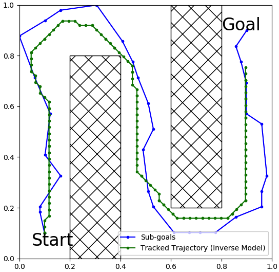
(a)

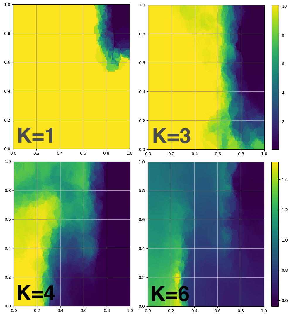
(b)

Figure 2: Batch RL experiment. (a) A robot needs to navigate between the (hatched) obstacles. Blue - SGT prediction, green - trajectory tracking sub-goals using an inverse model. (b) Approximate values $\hat{V}_{k}(s,g=[0.9,0.9])$ for several values of $k$. Note how the reachable region to the goal (non-yellow) grows with $k$.

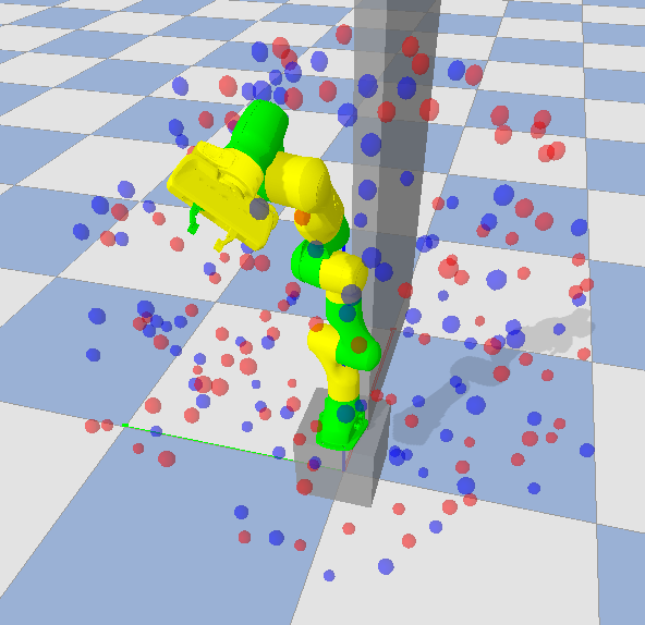
(a)

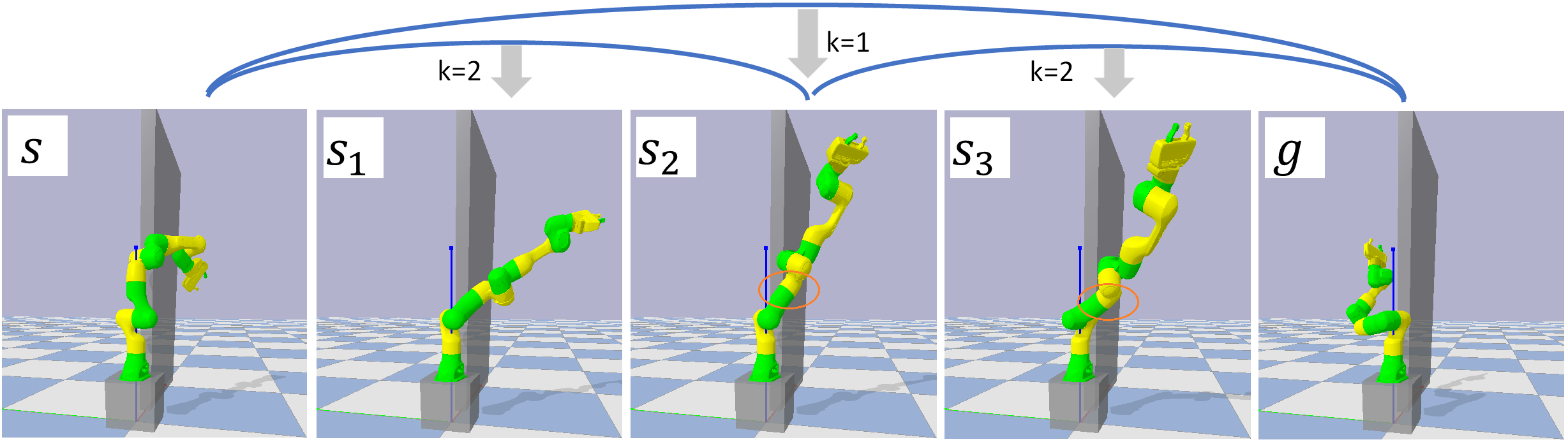
(b)

Figure 3: Motion planning with SGT-PG. (a) Illustration of start (red) and goal (blue) positions of the end effector in wall domain. (b) SGT Trajectory. Note a non-trivial rotation between $s_{2}$ to $s_{3}$ (marked with orange circles) allowing linear motion from $s_{3}$ to $g$. In the supplementary material we also show a 7 sub-goals path.

6.1 Fitted SGTDP Experiments

We start by evaluating the Fitted SGTDP algorithm. We consider a 2D particle moving in an environment with obstacles, as shown in Figure 2(a). The particle can move a distance of $0.025$ in one of the eight directions, and suffers a constant cost of $0.025$ in free space, and a large cost of $10$ on collisions. Its task is reaching from any starting point to within a $0.15$ distance of any goal point without collision. This simple domain is a continuous-state optimal control Problem (2), and for distant start and goal points, as shown in Figure 2(a), it requires relatively long-horizoned planning, making it suitable for studying batch RL algorithms.

To generate data, we sampled states and actions uniformly and independently, resulting in $125$K $(s,u,c,s^{\prime})$ tuples. As for function approximation, we opted for simplicity, and used K-nearest neighbors (KNN) for all our experiments, with K${}_{neighbors}=5$. To solve the minimization over states in Fitted SGTDP, we discretized the state space and searched over a $50\times 50$ grid of points.

A natural baseline in this setting is FQI (Ernst et al., 2005; Riedmiller, 2005). We verified that for a fixed goal, FQI obtains near perfect results with our data. Then, to make it goal-conditioned, we used a universal Q-function (Schaul et al., 2015), requiring only a minor change in the algorithm (see supplementary for pseudo-code).

To evaluate the different methods, we randomly chose 200 start and goal points, and measured the distance from the goal the policies reach, and whether they collide with obstacles along the way. For FQI, we used the greedy policy with respect to the learned Q function. The approximate SGTDP method, however, does not automatically provide a policy, but only a state trajectory to follow. Thus, we experimented with two methods for extracting a policy from the learned sub-goal tree. The first is training an inverse model $f_{IM}(s,s^{\prime})$ – a mapping from $s,s^{\prime}$ to $u$, using our data, and the same KNN function approximation. To reach a sub-goal $g$ from state $s$, we simply run $f_{IM}(s,g)$ until we are close enough to $g$ (we set the threshold to $0.15$). An alternative method is first using FQI to learn a goal-based policy, as described above, and then running this policy on the sub-goals. The idea here is that the sub-goals learned by approximate SGTDP can help FQI overcome the long-horizon planning required in this task. Note that all methods use exactly the same data, and the same function approximation (KNN), making for a fair comparison.

In Table 1 we report our results. FQI only succeed in reaching the very closest goals, resulting in a high average distance to goal. Fitted SGTDP (approx. SGTDP+IM), on the other hand, computed meaningful sub-goals for almost all test cases, resulting in a low average distance to goal when tracked by the inverse model. Figure 2 shows an example sub-goal tree and a corresponding tracked trajectory. The FQI policy did learn not to hit obstacles, resulting in the lowest collision rate. This is expected, as colliding leads to an immediate high cost, while the inverse model is not trained to take cost into account. Interestingly, combining the FQI policy with the sub-goals improves both long-horizon planning and short horizoned collision avoidance. In Figure 2(b) we plot the approximate value function $\hat{V}_{k}$ for different $k$ and a specific goal at the top right corner. Note how the reachable parts of the state space to the goal expand with $k$.

	Avg. Distance to Goal	Avg. Collision Rate
approx. SGTDP + IM	0.13	0.25
approx. SGTDP + FQI	0.29	0.06
FQI	0.58	0.02

Table 1: Results for controllers of batch-RL experiments.

6.2 Neural Motion Planning

An interesting application domain for our approach is neural motion planning (NMP, Qureshi et al., 2018) – learning to predict collision-free trajectories for a robot among obstacles. Here, we study NMP for the 7DoF Franka Panda robotic arm. Due to lack of space, full technical details of this section appear in supplementary Section E.1.

We follow an RL approach to NMP (Jurgenson & Tamar, 2019), using a cost function that incentivizes short, collision-free trajectories that reach the goal. The state space is the robot’s 7 joint angles, and actions correspond to predicting the next state in the plan. Given the next predicted state, the robot moves by running a fixed PID controller in simulation, tracking a linear joint motion from current to next state, and a cost is incurred based on the resulting motion.

We formulate NMP as approximate APSP as follows. A model predicts $T-1$ sub-goals, resulting in $T$ motion segments. Those segments are executed and evaluated independently, i.e. when evaluating segment $(s,s^{\prime})$ the robot first resets to $s$, and the resulting cost is based on its travel to $s^{\prime}$.

Our experiments include two scenarios: self-collision and wall. In self-collision, there are no obstacles and the challenge is to generate a minimal distance path while avoiding self-collisions between the robot links. The more challenging wall workspace contains a wall that partitions the space in front of the robot (see Figure 3). In wall, the shortest path is often nonmyopic, requiring to first move away from the goal in order to pass the obstacle.

We compare SGT-PG with a sequential baseline, Sequential sub-goals (SeqSG), which prescribes the sub-goals predictions sequentially. For appropriate comparison, both models use a PPO objective (Schulman et al., 2017), and a fixed architecture neural network to model the policy. All other hyper-parameters were specifically tuned for each model.

Model	# Sub- goals	self- collision	wall
SGT-PG	1	1.$\pm$0.	0.896$\pm$0.016
	3	1.$\pm$0.	0.973$\pm$0.007
	7	0.996$\pm$0.007	0.973$\pm$0.007
SeqSG	1	1.$\pm$0.	0.676$\pm$0.034
	3	0.983$\pm$0.007	0.593$\pm$0.047
	7	0.88$\pm$0.03	0.487$\pm$0.037

Table 2: Success rates for the NMP scenarios.

Table 2 compares SGT-PG and SeqSG, on predictions of 1, 3, and 7 sub-goals. We evaluate success rate (reaching goal without collision) on 100 random start-goal pairs that were held out during training (see Figure 3a). Each experiment was repeated 3 times and the mean and range are reported. Note that only 1 sub-goal is required to solve self-collision, and both models obtain perfect scores. For wall, on the other hand, more sub-goals are required, and here SGT significantly outperforms SeqSG, which was not able to accurately predict several sub-goals.

7 Conclusion

We presented a framework for multi-goal RL that is derived from a novel first principle – the SGT dynamic programming equation. For deterministic domains, we showed that SGTs are less prone to drift due to approximation errors, reducing error accumulation from $O(N^{2})$ to $O(N\log N)$. We further developed value-based and policy gradient RL algorithms for SGTs, and demonstrated that, in line with their theoretical advantages, SGTs demonstrate improved performance in practice.

Our work opens exciting directions for future research, including: (1) can our approach be extended to stochastic environments? (2) how to explore effectively based on SGTs? (3) can SGTs be extended to image-based tasks? Finally, we believe that our ideas will be important for robotics and autonomous driving applications, and other domains where goal-based predictions are important.

Appendix A Proofs

Proof of Theorem 1

Proof.

First, by definition, the shortest path from $s$ to itself is $0$. In the following, therefore, we assume that $s\neq s^{\prime}$.

We show by induction that each $V_{k}(s,s^{\prime})$ in Algorithm (4) is the cost of the shortest path from $s$ to $s^{\prime}$ in $2^{k}$ steps or less.

Let $\tau_{k}(s,s^{\prime})$ denote a shortest path from $s$ to $s^{\prime}$ in $2^{k}$ steps or less, and let $V_{k}(s,s^{\prime})$ denote its corresponding cost. Our induction hypothesis is that $V_{k-1}(s,s^{\prime})$ is the cost of the shortest path from $s$ to $s^{\prime}$ in $2^{k-1}$ steps or less. We will show that $V_{k}(s,s^{\prime})=\min_{s_{m}}\left\{V_{k-1}(s,s_{m})+V_{k-1}(s_{m},s^{\prime})\right\}$.

Assume by contradiction that there was some $s^{*}$ such that $V_{k-1}(s,s^{*})+V_{k-1}(s^{*},s^{\prime})<V_{k}(s,s^{\prime})$. Then, the concatenated trajectory $[\tau_{k-1}(s,s^{*}),\tau_{k-1}(s^{*},s^{\prime})]$ would have $2^{k}$ steps or less, contradicting the fact that $\tau_{k}(s,s^{\prime})$ is a shortest path from $s$ to $s^{\prime}$ in $2^{k}$ steps or less. So we have that $V_{k}(s,s^{\prime})\leq\left\{V_{k-1}(s,s_{m})+V_{k-1}(s_{m},s^{\prime})\right\}\quad\forall s_{m}$. Since the graph is complete, $\tau_{k}(s,s^{\prime})$ can be split into two trajectories of length $2^{k-1}$ steps or less. Let $s_{m}$ be a midpoint in such a split. Then we have that $V_{k}(s,s^{\prime})=\left\{V_{k-1}(s,s_{m})+V_{k-1}(s_{m},s^{\prime})\right\}$. So equality can be obtained and thus we must have $V_{k}(s,s^{\prime})=\min_{s_{m}}\left\{V_{k-1}(s,s_{m})+V_{k-1}(s_{m},s^{\prime})\right\}$.

To complete the induction argument, we need to show that $V_{0}(s,s^{\prime})=c(s,s^{\prime})$. This holds since for $k=0$, for each $s,s^{\prime}$, the only possible trajectory between them of length $1$ is the edge $s,s^{\prime}$.

Finally, since there are no negative cycles in the graph, for any $s,s^{\prime}$, the shortest path has at most $N$ steps. Thus, for $k=\log_{2}(N)$, we have that $V_{k}(s,s^{\prime})$ is the cost of the shortest path in $N$ steps or less, which is the shortest path between $s$ and $s^{\prime}$. ∎

Proof of Proposition 1

Proof.

The SGTDP Operator T is non-linear and not a contraction, but it is monotonic:

$$\forall s,g:V_{\alpha}(s,g)\leq V_{\beta}(s,g)\rightarrow\forall s,g:TV_{\alpha}(s,g)\leq TV_{\beta}(s,g).$$ (11)

To show (11), let $s_{m}^{\prime}=\arg\min_{s_{m}}{\{V_{\beta}(s,s_{m})+V_{\beta}(s_{m},g)\}}$. Then:

$$TV_{\alpha}(s,g) =\min_{s_{m}}{\{V_{\alpha}(s,s_{m})+V_{\alpha}(s_{m},g)\}}\leq V_{\alpha}(s,s_{m}^{\prime})+V_{\alpha}(s_{m}^{\prime},g)$$

$$\leq V_{\beta}(s,s_{m}^{\prime})+V_{\beta}(s_{m}^{\prime},g)=\min_{s_{m}}{\{V_{\beta}(s,s_{m})+V_{\beta}(s_{m},g)\}}=TV_{\beta}(s,g)$$

Back to the proof. By denoting $e=(1,1,1,1,...,1)$ we can write (6) as:

$$V_{0}-e\epsilon\leq\hat{V_{0}}\leq V_{0}+e\epsilon$$

Since T is monotonic, we can apply it on the inequalities:

$$T(V_{0}-e\epsilon)\leq T\hat{V_{0}}\leq T(V_{0}+e\epsilon)$$

Focusing on the left-hand side expression (the right-hand side is symmetric) we obtain:

$$T(V_{0}-e\epsilon)(s,s^{\prime})=\min_{s_{m}}\left\{(V_{0}-e\epsilon)(s,s_{m})+(V_{0}-e\epsilon)(s_{m},s^{\prime})\right\}=\min_{s_{m}}\left\{V_{0}(s,s_{m})+V_{0}(s_{m},s^{\prime})-2\epsilon\right\}=TV_{0}(s,s^{\prime})-2\epsilon$$

leading to:

$$TV_{0}-2e\epsilon\leq T\hat{V_{0}}\leq TV_{0}+2e\epsilon$$

Using (6):

$$TV_{0}-(2+1)e\epsilon\leq T\hat{V_{0}}-e\epsilon\leq\hat{V_{1}}\leq T\hat{V_{0}}+e\epsilon\leq TV_{0}+(2+1)e\epsilon$$

Proceeding similarly we obtain for $\hat{V_{2}}$:

$$T^{2}V_{0}-[2(2+1)+1]e\epsilon\leq\hat{V_{2}}\leq T^{2}V_{0}+[2(2+1)+1]e\epsilon$$

And for every $k\geq 1$:

$$T^{k}V_{0}-(2^{k+1}-1)e\epsilon\leq\hat{V_{k}}\leq T^{k}V_{0}+(2^{k+1}-1)e\epsilon$$

$$\|\hat{V}_{k}-V_{k}\|_{\infty}=\|\hat{V}_{k}-T^{k}V_{0}\|_{\infty}\leq(2^{k+1}-1)\epsilon$$ (12)

For $k=\log_{2}{N}$ we obtain:

$$\|\hat{V}_{\log_{2}{N}}-V^{*}\|_{\infty}=\|\hat{V}_{\log_{2}{N}}-V_{\log_{2}{N}}\|_{\infty}\leq\epsilon(2N-1)$$

∎

Proof of Proposition 2

Proof.

For every iteration $k$, the middle state of any greedy SGT path with length $2^{k}$ is $\hat{s}_{m}=\operatorname*{arg\,min}_{s_{m}}\left\{\hat{V}_{k-1}(s,s_{m})+\hat{V}_{k-1}(s_{m},g)\right\}$. Thereby $\hat{s}_{m}$ fulfils the identity $\hat{V}_{k-1}(s,\hat{s}_{m})+\hat{V}_{k-1}(\hat{s}_{m},g)=T\hat{V}_{k-1}(s,g)$, for every iteration $k$, where $T$ is the SGT operator. The next two relations then follow:

$$|\hat{V}_{k-1}(s,\hat{s}_{m})+\hat{V}_{k-1}(\hat{s}_{m},g)-V_{k}(s,g)| =|T\hat{V}_{k-1}(s,g)-V_{k}(s,g)|\leq$$

$$\leq|T\hat{V}_{k-1}(s,g)-\hat{V}_{k}(s,g)|+|\hat{V}_{k}(s,g)-V_{k}(s,g)|\leq$$ (13)

$$\leq\epsilon+(2^{k+1}-1)\epsilon=2^{k+1}\epsilon$$

$$|V_{k-1}(s,\hat{s}_{m})+V_{k-1}(\hat{s}_{m},g)-V_{k}(s,g)|\leq |\hat{V}_{k-1}(s,\hat{s}_{m})+\hat{V}_{k-1}(\hat{s}_{m},g)-V_{k}(s,g)|+$$

$$+|V_{k-1}(s,\hat{s}_{m})-\hat{V}_{k-1}(s,\hat{s}_{m})|+$$ (14)

$$+|V_{k-1}(\hat{s}_{m},g)-\hat{V}_{k-1}(\hat{s}_{m},g)|\leq$$

$$\leq |\hat{V}_{k-1}(s,\hat{s}_{m})+\hat{V}_{k-1}(\hat{s}_{m},g)-V_{k}(s,g)|+2\cdot(2^{k}-1)\epsilon$$

Combining the two inequalities yields:

$$|V_{k-1}(s,\hat{s}_{m})+V_{k-1}(\hat{s}_{m},g)-V_{k}(s,g)|\leq(2^{k+1}+2\cdot(2^{k}-1))\epsilon\leq 2^{k+2}\epsilon$$ (15)

Explicitly writing down relation (15) for all the different sub-paths we obtain:

$$|V_{\log_{2}(N/2)}(s_{0},s_{N/2}) +V_{\log_{2}(N/2)}(s_{N/2},s_{N}) -V_{\log_{2}(N)}(s_{0},s_{N}) |\leq 4N\epsilon$$

$$|V_{\log_{2}(N/4)}(s_{0},s_{N/4}) +V_{\log_{2}(N/4)}(s_{N/4},s_{N/2}) -V_{\log_{2}(N/2)}(s_{0},s_{N/2}) |\leq 2N\epsilon$$

$$|V_{\log_{2}(N/4)}(s_{N/2},s_{3N/4}) +V_{\log_{2}(N/4)}(s_{3N/4},s_{N}) -V_{\log_{2}(N/2)}(s_{N/2},s_{N}) |\leq 2N\epsilon$$

$$|V_{\log_{2}(N/8)}(s_{0},s_{N/8}) +V_{\log_{2}(N/8)}(s_{N/8},s_{N/4}) -V_{\log_{2}(N/4)}(s_{0},s_{N/4}) |\leq N\epsilon$$

$$|V_{\log_{2}(N/8)}(s_{N/4},s_{3N/8}) +V_{\log_{2}(N/8)}(s_{3N/8},s_{N/2}) -V_{\log_{2}(N/4)}(s_{N/4},s_{N/2}) |\leq N\epsilon$$

$$|V_{\log_{2}(N/8)}(s_{N/2},s_{5N/8}) +V_{\log_{2}(N/8)}(s_{5N/8},s_{3N/4}) -V_{\log_{2}(N/4)}(s_{N/2},s_{3N/4}) |\leq N\epsilon$$

$$|V_{\log_{2}(N/8)}(s_{3N/4},s_{7N/8}) +V_{\log_{2}(N/8)}(s_{7N/8},s_{N}) -V_{\log_{2}(N/4)}(s_{3N/4},s_{N}) |\leq N\epsilon$$

⋮

$$|V_{0}(s_{0},s_{1}) +V_{0}(s_{1},s_{2}) -V_{1}(s_{0},s_{2}) |\leq 8\epsilon$$

$$|V_{0}(s_{2},s_{3}) +V_{0}(s_{3},s_{4}) -V_{1}(s_{2},s_{4}) |\leq 8\epsilon$$

⋮

$$|V_{0}(s_{N-2},s_{N-1}) +V_{0}(s_{N-1},s_{N}) -V_{1}(s_{N-2},s_{N}) |\leq 8\epsilon$$

Summing all the inequalities, along with the triangle inequality, lead to the following:

$$|\sum_{i=0}^{N-1}V_{0}(s_{i},s_{i+1})-V_{\log_{2}(N)}(s_{0},s_{N})|\leq 4N\log_{2}{(N)}\epsilon$$

The identities $c(s_{i},s_{i+1})=V_{0}(s_{i},s_{i+1})$ and $V^{*}(s_{0},s_{N})=V_{\log_{2}{N}}(s_{0},s_{N})$ complete the proof. ∎

Proposition 2 provides a bound on the approximate shortest path using SGTDP. In contrast, we show that a similar bound for the sequential Bellman approach does not hold. For a start and goal pair $s,g$, and an approximate Bellman value function $\hat{V}^{B}$, let $s_{0}^{B},\dots,s_{N}^{B}$ denote the greedy shortest path according to the Bellman operator, i.e., $s_{0}=s,s_{N}=g$ and for $1\leq k<N$: $s_{k+1}=\operatorname*{arg\,min}_{s_{m}}\left\{c(s_{k},s_{m})+\hat{V}^{B}(s_{m},g)\right\}$. Note that the greedy Bellman update is not guaranteed to generate a trajectory that reaches the goal, therefore we add $g$ as the last state in the trajectory, following our convention that the graph is fully connected. When evaluating the greedy trajectory error in the sequential approach, we deal with two different implementation cases: Using one approximated value function or $N$ approximated value functions. The next proposition shows that when using one value function the greedy trajectory can be arbitrarily bad, regardless of $\epsilon$. Propositions (4) and (5) show that the error of the greedy trajectory, using $N$ value functions, have a tight $\mathcal{O}(N^{2})$ bound.

Proposition 3.

For any $\epsilon,\beta$, there exists a graph and an approximate value function $\hat{V}^{B}$ satisfying $\|\hat{V}^{B}-V^{*}\|_{\infty}\leq\epsilon N$, such that $\sum_{i=0}^{N-1}c(s_{i},s_{i+1})\geq V^{*}(s,g)+\beta$.

Proof.

We show a graph example (Figure 4), where a $\epsilon$-approximate Bellman value function $\hat{V}^{B}$ might form the path $s_{0},s_{0},\dots,s_{0},g$ with a total cost of infinity. (Reminder: The graph is fully connected, all the non-drawn edges have infinity cost), while the optimal path $s_{0},s_{1},\dots,s_{N-1},g$ has a total cost of $N\epsilon$.
As $\hat{V}^{B}$ is independent of the current time-step $k$, and the optimal values for $s$ and $s_{1}$ are $N\epsilon$ and $(N-1)\epsilon$ respectively, due to approximation error $\hat{V}^{B}$ (for every time-step) might suggest that the value of $s_{0}$ is lower than the value of $s_{1}$: $\hat{V}^{B}(s_{0},g)-N\epsilon\leq\hat{V}^{B}(s_{1},g)+N\epsilon$. The resulting policy will choose to stay in $s_{0}$ for the first $N-1$ steps. Since the maximum path length is $N$ and the path must end at the goal, the last step will be directly from $s_{0}$ to $g$, resulting in a cost of infinity.

∎

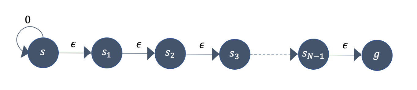
Figure 4: Example graph with a start and goal states $s,g$ where the optimal path has a total cost of $N\epsilon$ while $\epsilon$-approximated Bellman might form a path with total cost of infinity

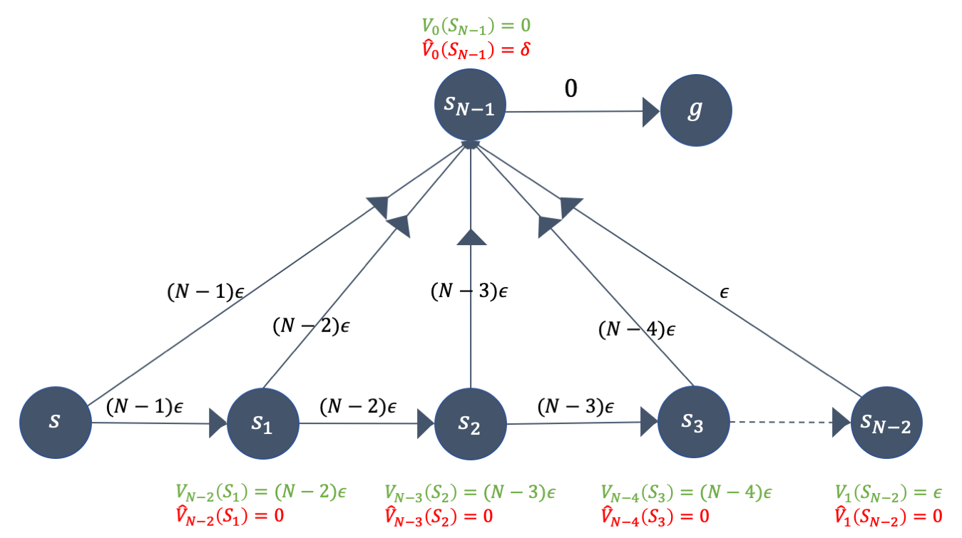
Figure 5: Example graph with a start and goal states $s,g$. The edges costs are marked in black labels, the Bellman value function at iteration k is marked in green and the $\epsilon$-approximated Bellman value is marked in red. The optimal path has a total cost of $V^{*}(s,g)=(N-1)\epsilon$ while the $\epsilon$-approximated Bellman might form the path going through all the states with a total cost of ${N^{2}-N}\epsilon/2=V^{*}(s,g)+\mathcal{O}(N^{2})$.

Proposition 4.

For a finite state graph, start and goal pair $s,g$, and sequence of $\epsilon$-approximate Bellman value functions $\hat{V}^{B}_{0},\dots,\hat{V}^{B}_{N}$ satisfying $\|\hat{V}^{B}_{k+1}-T^{B}\hat{V}^{B}_{k}\|_{\infty}\leq\epsilon$ and $\|\hat{V}^{B}_{0}-V_{0}\|_{\infty}\leq\epsilon$, let $s_{0},\dots,s_{N}$ denote the greedy Bellman path, that is: $s_{0}=s,s_{N}=g,s_{k+1}=\operatorname*{arg\,min}_{s_{k+1}}c(s_{k},s_{k+1})+\hat{V}^{B}_{N-k-2}(s_{k+1},g),$ etc. We have that $\sum_{i=0}^{N-1}c(s_{i},s_{i+1})\leq V^{*}(s,g)+(N^{2}-N)\epsilon=V^{*}(s,g)+\mathcal{O}(N^{2})$.

Proof.

Denote $V_{k}$ as the Bellman value function at iteration $k$, $\hat{V}_{k}$ as the $\epsilon$-approximated Bellman value function and $T_{B}$ as the Bellman operator. Using the properties $\|T_{B}\hat{V}_{k-1}-\hat{V_{k}}\|_{\infty}\leq\epsilon$ and $\|V_{k}-\hat{V_{k}}\|_{\infty}\leq k\epsilon$  (Bertsekas & Tsitsiklis, 1996, Pg. 332), the following relation holds:

for $0\leq k\leq N-2$:

$$c(s_{k},s_{k+1}) =c(s_{k},s_{k+1})+\hat{V}_{N-k-2}(s_{k+1},g)-\hat{V}_{N-k-2}(s_{k+1},g)$$

$$=(T_{B}\hat{V}_{N-k-2})(s_{k},g)-\hat{V}_{N-k-2}(s_{k+1},g)$$

$$\leq(\hat{V}_{N-k-1}(s_{k},g)+\epsilon)-\hat{V}_{N-k-2}(s_{k+1},g)$$

$$\leq V_{N-k-1}(s_{k},g)+(N-k-1)\epsilon+\epsilon-V_{N-k-2}(s_{k+1},g)+(N-k-2)\epsilon$$

$$\leq V_{N-k-1}(s_{k},g)-V_{N-k-2}(s_{k+1},g)+2(N-k-1)\epsilon$$

for $k=N-1$:

$$c(s_{k},s_{k+1}) =c(s_{N-1},g)=V_{0}(s_{N-1},g)$$

Summing all the path costs:

$$\sum_{k=0}^{N-1}c(s_{k},s_{k+1}) =V_{0}(s_{N-1},g)+\sum_{k=0}^{N-2}c(s_{k},s_{k+1})$$

$$\leq V_{0}(s_{N-1},g)+\sum_{k=0}^{N-2}V_{N-k-1}(s_{k},g)-V_{N-k-2}(s_{k+1},g)+2(N-k-1)\epsilon$$

$$=V_{0}(s_{N-1},g)+V_{N-1}(s_{0},g)-V_{0}(s_{N-1},g)+(N^{2}-N)\epsilon=V^{*}(s_{0},g)+(N^{2}-N)\epsilon$$

∎

Proposition 5.

The error bound stated in Proposition(4), $\sum_{i=0}^{N-1}c(s_{i},s_{i+1})-V^{*}(s,g)\leq\mathcal{O}(N^{2})$, is indeed a tight bound.

Proof.

We show a graph example (Figure 5),where a sequence of $\epsilon$-approximate Bellman value functions $\hat{V}_{0},\dots,\hat{V}_{N-1}$ might form the path from the start to the goal state, going through all the available states, with a total cost of $(N^{2}-N)/2=\mathcal{O}(N^{2})$, while the optimal path $(s_{0},s_{N-1},s_{N})$ has a total cost of $V^{*}(s,g)=(N-1)\epsilon$.
The Bellman value of every state $s_{k}$, $0\leq k\leq s_{N-3}$: $V_{N-k-1}(s_{k},g)=(N-k-1)\epsilon$, where $N-k-1$ is the time horizon from state $s_{k}$ to the goal. Since the $\epsilon$-approximate Bellman value function at every state $s_{k}$ might have a maximum approximation error of $(N-k-1)\epsilon$, it might suggest that $\hat{V}_{N-k-1}(s_{k},g)=0$ for every $1\leq k\leq N-2$. The Bellman value for state $s_{N-1}$ is 0 and the $\epsilon$-approximate Bellman value might be $\delta$ for some $0<\delta\leq\epsilon$. The greedy Bellman policy has to determine at every state $s_{k}$, $0\leq k\leq s_{N-3}$, whether to go to $s_{k+1}$ or to $s_{N-1}$. Since both possible actions have an immediate cost of $(N-k-1)\epsilon$, the decision will only be based on the evaluation of $s_{k+1}$ and $s_{N-1}$ with the $\epsilon$-approximate Bellman value function: $\hat{V}_{N-k-1}(s_{k},g)=0<\delta=\hat{V}_{0}(s_{N-1},g)$. Therefore, the greedy bellman policy will decide at every state $s_{k}$ to go to $s_{k+1}$, forming the path with a total cost of $\sum_{k=1}^{N-1}k\epsilon={N^{2}-N}\epsilon/2$
∎

Appendix B Policy Gradient Theorem for Sub-goal Trees

In this section we provide the mathematical framework and tool we used in the Policy Gradient Theorem 2 in Section 5.2 which allows us to formulate the SGT-PG algorithm (Section 5.2). The SGT the prediction process (Eq.(8)) no-longer decomposes sequentially like a MDP, therefore, we provide a different mathematical construct:

Finite-depth Markovian sub-goal tree (FD-MSGT) is a process predicting sub-goals (or intermediate states) of a trajectory in a dynamical system as described in (3). The process evolves trajectories recursively (as we describe in detail below), inducing a tree-like decomposition for the probability of a trajectory as described Eq. (8). In this work we consider trees with fixed levels $D$ (corresponding to finite-horizon MDP in sequential prediction RL with horizon $T=2^{D}$) . Formally, a FD-MSGT is comprised of $(S,\rho_{0},c,D)$ where $S$ is the state space, $\rho_{0}$ is the initial start-goal pairs distribution, $c$ is a non-negative cost function obeying Eq. (3), and $D$ is the depth of the tree .

Recursive evolution of FD-MSGT: Formally, an initial pair $(s_{0}=s,s_{T}=g)\sim\rho_{0}$ is sampled, defining the root of the tree. Next, a policy $\pi(s_{\frac{T}{2}}|s_{0},s_{T})$ is used to predict the sub-goal $s_{\frac{T}{2}}$, creating two new tree nodes of depth $D$ corresponding to the segments $(s_{0},s_{\frac{T}{2}})$ and $(s_{\frac{T}{2}},s_{T})$. Recursively each segment is again partitioned using $\pi$ resulting in four tree nodes of level $D-1$ corresponding to segments $(s_{0},s_{\frac{T}{4}})$, $(s_{\frac{T}{4}},s_{\frac{T}{2}})$, $(s_{\frac{T}{2}},s_{\frac{3T}{4}})$ and $(s_{\frac{3T}{4}},s_{T})$. The process continues recursively until the depth of the tree is $1$. This results in Eq.(8), namely,

$$\Pr_{\pi}[\tau|s,g]=\Pr_{\pi}[s_{0},\dots,s_{T}|s,g]=\Pr_{\pi}[s_{0},\dots,s_{\frac{T}{2}}|s,s_{m}]\Pr_{\pi}[s_{\frac{T}{2}},\dots,s_{T}|s_{m},g]\pi(s_{m}|s,g).$$

FD-MSGT results in $\sum_{d=0}^{D-1}{2^{d}}=2^{D}-1$ sub-goals, and $2^{D}+1$ overall states (including $s$ and $g$), setting $T=2^{D}$. Finally, $c$ defines the cost of the prediction $c(\tau)=c_{0:T}$, and is evaluated on the leaves of the FD-MSGT tree according to Eq. (3). Figure 3(b) illustrates a FD-MSGT of $D=2$. The objective of FD-MSGT is to find a policy $\pi:S^{2}\rightarrow S$ minimizing the expected cost of a trajectory $J^{\pi}=\mathbb{E}_{\tau\sim\rho(\pi)}\left[c_{\tau}\right]$.

Non-recursive formulation for trajectory likelihood: We next derive a non-recursive formulation of Eq. (8), using the notations defined in Theorem 2, namely, $s^{i,d}=s_{(i-1)\cdot 2^{d}}$, $s_{m}^{i,d}=s_{(2i-1)\cdot 2^{d-1}}$, $g^{i,d}=s_{i\cdot 2^{d}}$, and $C_{\tau}^{i,d}=c_{(i-1)\cdot 2^{d}:i\cdot 2^{d}}$ is the sum of costs from $s^{i,d}$ to $g^{i,d}$ of $\tau$. We re-arrange the terms in (8) grouping by depth resulting in a non-recursive formula,

$$\Pr_{\pi}[\tau|s,g]=\Pr_{\pi}[s_{0},\dots s_{T}|s,g]=\prod_{d=1}^{D}{\prod_{i=1}^{2^{D-d}}{\pi\left(s_{m}^{i,d}\bigg{|}s^{i,d},g^{i,d}\right).}}$$ (16)

For example consider a FD-MSGT with $D=3$ ($T=8)$. Given $s_{0}=s$ and $s_{8}=g$, the sub-goals will be $s_{1},\dots s_{7}$. We enumerate the two products in Eq. (16) resulting in:

1. $D=3$: Results in a single iteration of $i=1=2^{3-3}$.

   $$s^{1,3}=s_{(1-1)\cdot 2^{3}}=s_{0},\quad s_{m}^{1,3}=s_{(2\cdot 1-1)\cdot 2^{3-1}}=s_{4},\quad g^{1,3}=s_{1\cdot 2^{3}}=s_{8}$$

2. $D=2$: In this case $i\in[1,2^{3-2}=2]$.

   $$s^{1,2}=s_{(1-1)\cdot 2^{2}}=s_{0},\quad s_{m}^{1,2}=s_{(2\cdot 1-1)\cdot 2^{2-1}}=s_{2},\quad g^{1,2}=s_{1\cdot 2^{2}}=s_{4}$$

   $$s^{2,2}=s_{(2-1)\cdot 2^{2}}=s_{4},\quad s_{m}^{2,2}=s_{(2\cdot 2-1)\cdot 2^{2-1}}=s_{6},\quad g^{2,2}=s_{2\cdot 2^{2}}=s_{8}$$

3. $D=1$: Finally, predicts the leaves resulting in $i\in[1,2^{3-1}=4]$.

   $$s^{1,1}=s_{(1-1)\cdot 2^{1}}=s_{0},\quad s_{m}^{1,1}=s_{(2\cdot 1-1)\cdot 2^{1-1}}=s_{1},\quad g^{1,1}=s_{1\cdot 2^{1}}=s_{2}$$

   $$s^{2,1}=s_{(2-1)\cdot 2^{1}}=s_{2},\quad s_{m}^{2,1}=s_{(2\cdot 2-1)\cdot 2^{1-1}}=s_{3},\quad g^{2,1}=s_{2\cdot 2^{1}}=s_{4}$$

   $$s^{3,1}=s_{(3-1)\cdot 2^{1}}=s_{4},\quad s_{m}^{3,1}=s_{(2\cdot 3-1)\cdot 2^{1-1}}=s_{5},\quad g^{3,1}=s_{3\cdot 2^{1}}=s_{6}$$

   $$s^{4,1}=s_{(4-1)\cdot 2^{1}}=s_{6},\quad s_{m}^{4,1}=s_{(2\cdot 4-1)\cdot 2^{1-1}}=s_{7},\quad g^{4,1}=s_{4\cdot 2^{1}}=s_{8}$$

Allowing us to assert the equivalence of the explicit and recursive formulations in this case.

B.1 Proof of Theorem 2

Let $\pi_{\theta}$ be a policy with parameters $\theta$, we next prove a policy gradient theorem (Theorem 3) for computing $\nabla_{\theta}J^{\pi_{\theta}}$, using the following proposition:

Proposition 6.

Let $\pi_{\theta}$ be a policy with parameters $\theta$ of a FD-MSGT with depth $D$, then

$$\nabla_{\theta}\log{\Pr_{\rho(\pi_{\theta})}[\tau]}=\sum_{d=1}^{D}{\sum_{i=1}^{2^{D-d}}{\nabla_{\theta}\log{\pi_{\theta}\left(s_{m}^{i,d}\bigg{|}s^{i,d},g^{i,d}\right)}}}$$ (17)

Proof.

First, we express $\Pr_{\rho(\pi_{\theta})}[\tau]$ using Eq. 16 and $\rho_{0}$ obtaining,

$$\Pr_{\rho(\pi_{\theta})}[\tau]=\rho(s_{0},s_{T})\cdot\prod_{d=1}^{D}{\prod_{i=1}^{2^{D-d}}{\pi_{\theta}\left(s_{m}^{i,d}\bigg{|}s^{i,d},g^{i,d}\right).}}$$

Next, by taking the log we have,

$$\log{\Pr_{\rho(\pi_{\theta})}[\tau]}=\log{\rho(s_{0},s_{T})}+\sum_{d=1}^{D}{\sum_{i=1}^{2^{D-d}}{\log{\pi_{\theta}\left(s_{m}^{i,d}\bigg{|}s^{i,d},g^{i,d}\right)}}}.$$

and taking the gradient w.r.t $\theta$ yields Eq. (17) ∎

Proposition 6 shows that the gradient of a trajectory w.r.t. $\theta$ does not depend on the initial distribution. This allows us to derive a policy gradient theorem:

Theorem 3.

Let $\pi_{\theta}$ be a stochastic SGT policy, $\rho(\pi_{\theta})$ be a trajectory distribution defined above, and $T=2^{D}$. Then

$$\nabla_{\theta}J(\theta)=\mathbb{E}_{\rho(\pi_{\theta})}\left[c_{\tau}\cdot\nabla_{\theta}\log{\Pr_{\rho(\pi_{\theta})}[\tau]}\right]=\mathbb{E}_{\rho(\pi_{\theta})}\left[c_{\tau}\cdot\sum_{d=1}^{D}{\sum_{i=1}^{2^{D-d}}{\nabla_{\theta}\log{\pi_{\theta}\left(s_{m}^{i,d}\bigg{|}s^{i,d},g^{i,d}\right)}}}\right]\!.$$

Proof.

To obtain $\nabla_{\theta}J(\theta)$ we write Eq. (9) as an explicit expectation and use $\nabla_{x}f(x)=f(x)\cdot\nabla_{x}\log{f(x)}$:

$$\nabla_{\theta}J(\theta)= \sum_{\tau}{c(\tau)\cdot\nabla_{\theta}\Pr_{\rho(\pi_{\theta})}[\tau]}=\sum_{\tau}{c(\tau)\cdot\Pr_{\rho(\pi_{\theta})}[\tau]\cdot\nabla_{\theta}\log{\Pr_{\rho(\pi_{\theta})}[\tau]}}=\mathbb{E}_{\rho(\pi_{\theta})}\left[c(\tau)\nabla_{\theta}\log{\Pr_{\rho(\pi_{\theta})}[\tau]}\right]$$

This proves the first equality. For the second equality we substitute $\nabla_{\theta}\log{\Pr_{\rho(\pi_{\theta})}[\tau]}$ according to Eq. (17). ∎

The policy gradient theorem allows estimating $\nabla J(\theta)$ from on policy data collected using $\pi_{\theta}$. We next show how to improve the estimate in Theorem 3 using control variates (baselines). We start with the following baseline-reduction proposition.

Proposition 7.

Let $\pi_{\theta}$ be a policy with parameters $\theta$ of a FD-MSGT with depth $D$, and let $b^{i,d}=b(s^{i,d},g^{i,d})$ be any fixed function $b^{i,d}:S^{2}\rightarrow R$, then

$$\mathbb{E}_{\rho(\pi_{\theta})}\left[\sum_{d=1}^{D}{\sum_{i=1}^{2^{D-d}}{b^{i,d}\cdot\nabla_{\theta}\log{\pi_{\theta}\left(s_{m}^{i,d}\bigg{|}s^{i,d},g^{i,d}\right)}}}\right]=0.$$ (18)

Proof.

First we establish a useful property. Let $p_{\theta}(z)$ be some parametrized distribution. Differentiating $\sum\nolimits_{z}{{p_{\theta}}(z)}=1$ yields

$$\sum\nolimits_{z}{(\nabla\log{p_{\theta}}({z})}){p_{\theta}}({z})={\mathbb{E}^{\theta}}(\nabla\log{p_{\theta}}({z}))=0.$$ (19)

Then we expand the left-hand side of Eq. (18), and use Eq. (19) in the last row:

$$\mathbb{E}_{\rho(\pi_{\theta})}\left[\sum_{d=1}^{D}{\sum_{i=1}^{2^{D-d}}{b^{i,d}\cdot\nabla_{\theta}\log{\pi_{\theta}\left(s_{m}^{i,d}\bigg{|}s^{i,d},g^{i,d}\right)}}}\right]= \sum_{d=1}^{D}{\sum_{i=1}^{2^{D-d}}{\mathbb{E}_{\rho(\pi_{\theta})}\left[b^{i,d}\cdot\nabla_{\theta}\log{\pi_{\theta}\left(s_{m}^{i,d}\bigg{|}s^{i,d},g^{i,d}\right)}\right]}}=$$

$$\sum_{d=1}^{D}{\sum_{i=1}^{2^{D-d}}{\mathbb{E}_{\rho(\pi_{\theta})}\left[\mathbb{E}_{\rho(\pi_{\theta})}\left[b^{i,d}\cdot\nabla_{\theta}\log{\pi_{\theta}\left(s_{m}^{i,d}\bigg{|}s^{i,d},g^{i,d}\right)}\big{|}s^{i,d},g^{i,d}\right]\right]}}=$$

$$\sum_{d=1}^{D}{\sum_{i=1}^{2^{D-d}}{\mathbb{E}_{\rho(\pi_{\theta})}\left[b^{i,d}\cdot\mathbb{E}_{\rho(\pi_{\theta})}\left[\nabla_{\theta}\log{\pi_{\theta}\left(s_{m}^{i,d}\bigg{|}s^{i,d},g^{i,d}\right)}\big{|}s^{i,d},g^{i,d}\right]\right]}}=$$

$$\sum_{d=1}^{D}{\sum_{i=1}^{2^{D-d}}{\mathbb{E}_{\rho(\pi_{\theta})}\left[b^{i,d}\cdot 0\right]}}=0,$$

which concludes the proof.

∎

We define $b:S^{2}\rightarrow R$ as a segment-dependent baseline if $b$ is a fixed function that operates on a pair of states $s$ and $g$. The last proposition allows us to reduce segment-dependent baselines, $b^{i,d}$, from the estimations of $\nabla J(\theta)$ without bias. Finally, in the next proposition we show that instead of estimating $\nabla J(\theta)$ using $c_{\tau}$ we can instead use $C^{i,d}$ as follows:

Proposition 8.

Let $\pi_{\theta}$ be a policy with parameters $\theta$ of a FD-MSGT with depth $D$, then:

$$\nabla_{\theta}J(\theta)=\sum_{d=1}^{D}{\sum_{i=1}^{2^{D-d}}{\mathbb{E}_{\rho(\pi_{\theta})}\left[c_{(i-1)\cdot 2^{d}:i\cdot 2^{d}}\cdot\nabla_{\theta}\log{\pi_{\theta}\left(s_{m}^{i,d}\bigg{|}s^{i,d},g^{i,d}\right)}\right]}}$$

Proof.

We have that:

$$\nabla_{\theta}J(\theta)= \mathbb{E}_{\rho(\pi_{\theta})}\left[c_{\tau}\cdot\sum_{d=1}^{D}{\sum_{i=1}^{2^{D-d}}{\nabla_{\theta}\log{\pi_{\theta}\left(s_{m}^{i,d}\bigg{|}s^{i,d},g^{i,d}\right)}}}\right]=\sum_{d=1}^{D}{\sum_{i=1}^{2^{D-d}}{\mathbb{E}_{\rho(\pi_{\theta})}\left[c_{\tau}\cdot\nabla_{\theta}\log{\pi_{\theta}\left(s_{m}^{i,d}\bigg{|}s^{i,d},g^{i,d}\right)}\right]}}$$

$$= \sum_{d=1}^{D}{\sum_{i=1}^{2^{D-d}}{\mathbb{E}_{\rho(\pi_{\theta})}\left[\mathbb{E}_{\rho(\pi_{\theta})}\left[c_{\tau}\cdot\nabla_{\theta}\log{\pi_{\theta}\left(s_{m}^{i,d}\bigg{|}s^{i,d},g^{i,d}\right)}\bigg{|}s_{0}\dots s^{i,d},g^{i,d}\dots s_{T}\right]\right]}}.$$ (20)

The first transition is the expectation of sums, and the second is the smoothing theorem. We next expand the inner expectation in Eq. (B.1), and partition the sum of cost $c_{\tau}$ into three sums: between indices $0$ to $(i-1)\cdot 2^{d}$, $(i-1)\cdot 2^{d}$ to $i\cdot 2^{d}$, and finally from $i\cdot 2^{d}$ to $T$.

$$\mathbb{E}_{\rho(\pi_{\theta})}\left[c_{\tau}\cdot\nabla_{\theta}\log{\pi_{\theta}\left(s_{m}^{i,d}\bigg{|}s^{i,d},g^{i,d}\right)}\bigg{|}s_{0}\dots s^{i,d},g^{i,d}\dots s_{T}\right]$$

$$=\mathbb{E}_{\rho(\pi_{\theta})}\left[\left(c_{0:(i-1)\cdot 2^{d}}+c_{i\cdot 2^{d}:T}\right)\cdot\nabla_{\theta}\log{\pi_{\theta}\left(s_{m}^{i,d}\bigg{|}s^{i,d},g^{i,d}\right)}\bigg{|}s_{0}\dots s^{i,d},g^{i,d}\dots s_{T}\right]$$

$$+\mathbb{E}_{\rho(\pi_{\theta})}\left[c_{(i-1)\cdot 2^{d}:i\cdot 2^{d}}\cdot\nabla_{\theta}\log{\pi_{\theta}\left(s_{m}^{i,d}\bigg{|}s^{i,d},g^{i,d}\right)}\bigg{|}s_{0}\dots s^{i,d},g^{i,d}\dots s_{T}\right].$$

Next, by the definition of FD-MSGT the costs between $s_{0}$ to $s_{(i-1)\cdot 2^{d}}$ and $s_{i\cdot 2^{d}}$ to $s_{T}$, are independent of the policy predictions between indices $(i-1)\cdot 2^{d}$ to $i\cdot 2^{d}$ – making them constants. As we showed in Proposition 7, we obtain that this expectation is 0. Thus the expression for $\nabla_{\theta}J(\theta)$ simplifies to:

$$\nabla_{\theta}J(\theta)= \sum_{d=1}^{D}{\sum_{i=1}^{2^{D-d}}{\mathbb{E}_{\rho(\pi_{\theta})}\left[\mathbb{E}_{\rho(\pi_{\theta})}\left[c_{\tau}\cdot\nabla_{\theta}\log{\pi_{\theta}\left(s_{m}^{i,d}\bigg{|}s^{i,d},g^{i,d}\right)}\bigg{|}s_{0}\dots s^{i,d},g^{i,d}\dots s_{T}\right]\right]}}$$

$$= \sum_{d=1}^{D}{\sum_{i=1}^{2^{D-d}}{\mathbb{E}_{\rho(\pi_{\theta})}\left[\mathbb{E}_{\rho(\pi_{\theta})}\left[c_{(i-1)\cdot 2^{d}:i\cdot 2^{d}}\cdot\nabla_{\theta}\log{\pi_{\theta}\left(s_{m}^{i,d}\bigg{|}s^{i,d},g^{i,d}\right)}\bigg{|}s_{0}\dots s^{i,d},g^{i,d}\dots s_{T}\right]\right]}}$$

$$= \sum_{d=1}^{D}{\sum_{i=1}^{2^{D-d}}{\mathbb{E}_{\rho(\pi_{\theta})}\left[c_{(i-1)\cdot 2^{d}:i\cdot 2^{d}}\cdot\nabla_{\theta}\log{\pi_{\theta}\left(s_{m}^{i,d}\bigg{|}s^{i,d},g^{i,d}\right)}\right]}}$$ (21)

∎

Finally, combining Propositions 7 and 8 in Theorem 3 provides us Theorem 2 in the main text.

Appendix C Batch RL Baselines

In Algorithm 3 we present a goal-based versions of fitted-Q iteration (FQI) (Ernst et al., 2005) using universal function approximation (Schaul et al., 2015), which we used as a baseline in our experiments.

Algorithm 3 Fitted Q with Universal Function Approximation

Algorithm 

      321 Input: dataset $D=\left\{s,u,c,s^{\prime}\right\}$, Goal reached threshold $\delta$
Create transition data set $D_{trans}=\left\{s,u,s^{\prime}\right\}$ and targets $T_{trans}=\left\{c\right\}$ with $s,s^{\prime},c$ taken from $D$
Fit $\hat{Q}(s,u,s^{\prime})$ to data in $D_{trans}$
for $k:1...K$ do

            54 Create random goal data set $D_{goal}=\left\{s,u,g\right\}$ and targets

$$T_{goal}=\left\{\left\{c(s,u)+\min_{u^{\prime}}\hat{Q}(s^{\prime},u^{\prime},g)_{||s^{\prime}-g||>\delta}\right\}\right\}$$

with $s,u,s^{\prime}$ taken from $D$ and $g$ randomly chosen from states in $D$
Fit $\hat{Q}(s,u,s^{\prime})$ to data in $D_{goal}$

       end for

      

Next, in Algorithm 4 we present an approximate dynamic programming version of Floyd-Warshall RL (Kaelbling, 1993) that corresponds to the batch RL setting we investigate. This algorithm was not stable in our experiments, as the value function converged to zero for all states (when removing the self transition fitting in line 7 of the algorithm, the values converged to a constant value).

Algorithm 4 Approximate Floyd Warshall

Algorithm 

      54321 Input: dataset $D=\left\{s,u,c,s^{\prime}\right\}$, Maximum path cost $C_{max}$
Create transition data set $D_{trans}=\left\{s,s^{\prime}\right\}$ and targets $T_{trans}=\left\{c\right\}$ with $s,s^{\prime},c$ taken from $D$
Create random transition data set $D_{random}=\left\{s,s_{rand}\right\}$ and targets $T_{random}=\left\{C_{max}\right\}$ with $s,s_{rand}$ randomly chosen from states in $D$
Create self transition data set $D_{self}=\left\{s,s\right\}$ and targets $T_{self}=\left\{0\right\}$ with $s$ taken from $D$
Fit $\hat{V}(s,s^{\prime})$ to data in $D_{trans},D_{random},D_{self}$
for $k:1...K$ do

            876 Create random goal and mid-point data set $D_{goal}=\left\{s,g\right\}$ and targets

$$T_{goal}=\left\{\min\left\{\hat{V}(s,g),\hat{V}(s,s_{m})+\hat{V}(s_{m},g)\right\}\right\}$$

with $s,s_{m},g$ randomly chosen from states in $D$
Create self transition data set $D_{self}=\left\{s,s\right\}$ and targets $T_{self}=\left\{0\right\}$ with $s$ taken from $D$
Fit $\hat{V}(s,s^{\prime})$ to data in $D_{goal},D_{self}$

       end for

      

Appendix D Learning SGT with Supervised Learning

In this section we describe how to learn SGT policies for deterministic, stationary, and finite time dynamical systems from labeled data generated by an expert. This setting is commonly referred to as Imitation Learning (IL). Specifically, we are given a dataset $D^{\pi^{*}}=\left\{\tau_{i}\right\}_{i=1}^{N}$ of $N$ trajectory demonstrations, provided by an expert policy $\pi^{*}$. Each trajectory demonstration $\tau_{i}$ from the dataset $D^{\pi^{*}}$, is a sequence of $T_{i}$ states, i.e. $\tau_{i}=s_{0}^{i},s_{1}^{i}\dots s_{T_{i}}^{i}$. In this work, we assume a goal-based setting, that is, we assume that the expert policy generates trajectories that lead to a goal state which is the last state in each trajectory demonstration. Our goal is to learn a policy that, given a pair of current state and goal state $(s,g)$, predicts the trajectory that $\pi^{*}$ would have chosen to reach $g$ from $s$.

D.1 Imitation learning with SGT

In this section, we describe the learning objectives for sequential and sub-goal tree prediction approaches under the IL settings. We focus on the Behavioral Cloning (BC)(Pomerleau, 1989) approach to IL, where a parametric model for a policy $\hat{\pi}$ with parameters $\theta$ is learned by maximizing the log-likelihood of observed trajectories in $D^{\pi^{*}}$, i.e.,

$$\theta^{*}=\arg\max_{\theta}{\mathbb{E}_{\tau_{i}\sim D^{\pi^{*}}}\left[\log P_{\hat{\pi}}(\tau_{i}=s_{0}^{i},s_{1}^{i},\dots s_{T}^{i}|s_{0}^{i},s_{T}^{i};\theta)\right]}.$$ (22)

Denote the horizon $T$ as the maximal number of states in a trajectory. For ease of notation we assume $T$ to be the same for all trajectories. Also, let $s_{i}=s_{0}^{i}$ and $g_{i}=s_{T_{i}}^{i}$ denote the start and goal states for $\tau_{i}$. We ask – how to best represent the distribution $P_{\hat{\pi}}(\tau|s,g;\theta)$?

The sequential trajectory representation (Pomerleau, 1989; Ross et al., 2011; Zhang et al., 2018; Qureshi et al., 2018), a popular approach, decomposes $P_{\hat{\pi}}(s_{0},s_{1},\dots s_{T}|s,g;\theta)$ by sequentially predicting states in the trajectory conditioned on previous predictions. Concretely, let $h_{t}=s_{0},s_{1},\dots,s_{t}$ denote the history of the trajectory at time index $t$, the decomposition assumed by the sequential representation is $P_{\hat{\pi}}(s_{0},s_{1},\dots s_{T}|s,g;\theta)=P_{\hat{\pi}}(s_{1}|h_{0},g;\theta)P_{\hat{\pi}}(s_{2}|h_{1},g;\theta)\dots P_{\hat{\pi}}(s_{T}|h_{T-1},g;\theta)$. Using this decomposition, (22) becomes:

$$\theta^{*}=\arg\max_{\theta}{\mathbb{E}_{\tau_{i}\sim D^{\pi^{*}}}\left[\sum_{t=1}^{T}{\log{P_{\hat{\pi}}(s_{t+1}^{i}|h_{t}^{i},g^{i};\theta)}}\right]}.$$ (23)

We can learn $P_{\hat{\pi}}$ using a batch stochastic gradient descent (SGD) method. To generate a sample $(s_{t},h_{t-1},g)$ in a training batch, a trajectory $\tau_{i}$ is sampled from $D^{\pi^{*}}$, and an observed state $s_{t}^{i}$ is further sampled from $\tau_{i}$. Next, the history $h_{t-1}^{i}$ and goal $g_{i}$ are extracted from $\tau_{i}$. After learning, sampling a trajectory between $s$ and $g$ is a straight-forward iterative process, where the first prediction is given by $s_{1}\sim P_{\hat{\pi}}(s|h_{0}=s,g;\theta)$, and every subsequent prediction is given by $s_{t+1}\sim P_{\hat{\pi}}(s|h_{t}=(s,s_{1},\dots s_{t}),g;\theta)$. This iterative process stops once some stopping condition is met (such as a target prediction horizon is reached, or a prediction is ’close-enough’ to $g$).

The Sub-Goal Tree Representation: In SGT we instead predict the middle-state in a divide-and-conquer approach. Following Eq. (8) we can redefine the maximum-likelihood objective as

$$\!\theta^{*}\!\!=\!\!\arg\max_{\theta}{\mathbb{E}_{\tau_{i}\sim D^{\pi^{*}}}\!\!\!\left[\log{P_{\hat{\pi}}(s_{T/2}^{i}|s^{i},g^{i};\theta)}\!\!+\!\log{P_{\hat{\pi}}(s_{T/4}^{i}|s^{i},s_{T/2}^{i};\theta)}\!\!+\!\log{P_{\hat{\pi}}(s_{3T/4}^{i}|s_{T/2}^{i},g^{i};\theta)}\!\dots\right]}.$$ (24)

To organize our data for optimizing Eq. (24), we first sample a trajectory $\tau_{i}$ from $D^{\pi^{*}}$ for each sample in the batch. From $\tau_{i}$ we sample two states $s_{a}^{i}$ and $s_{b}^{i}$ and obtain their midpoint $s_{\frac{a+b}{2}}^{i}$. Pseudo-code for sub-goal tree prediction and learning are provided in Algorithm 5 and Algorithm 6.

Algorithm 5 Sub-Goal Tree BC Trajectory Prediction

Algorithm 

      21 Input: parameters $\theta$ of parametric distribution $P_{\hat{\pi}}$, start state $s$, goal state $g$, max depth $K$
return [$s$] + PredictSGT($\theta$, $s$, $g$, $K$) +[$g$]

Procedure PredictSGT($\theta$, $s_{1}$, $s_{2}$, $k$)

       if $k>0$ then

            21 Predict midpoint $s_{m}\sim P_{\hat{\pi}}(s_{m}|s_{1},s_{2};\theta)$
return PredictSGT($\theta$, $s_{1}$, $s_{m}$, $k-1$) + [$s_{m}$] + PredictSGT($\theta$, $s_{m}$, $s_{2}$, $k-1$)

       end if

      

Algorithm 6 Sub-Goal Tree BC SGD-Based Training

Algorithm 

      21 Input: dataset $D=\left\{\tau_{i}=s_{0}^{i},s_{1}^{i}\dots s_{T_{i}}^{i}\right\}_{i=1}^{N}$, train steps $M$, batch size $B$
Initialize parameters $\theta$ for parametric distribution $P_{\hat{\pi}}(s_{m}|s,g;\theta)$
for $i:1...M$  do

            543 Sample batch of size $B$, each sample: $\tau_{i}\sim D$, $s_{1},s_{2}\sim\tau_{i}$
$s_{m}\leftarrow$ Get midpoint of $[s_{1},s_{2}]$ according to $\tau_{i}$ for all items in batch
Update $\theta$ by minimizing the negative log-likelihood loss:

$$L=-\frac{1}{B}\cdot\sum_{b=1}^{B}{\nabla_{\theta}\log{P_{\hat{\pi}}(s_{m}^{b}|s_{1}^{b},s_{2}^{b};\theta)}}$$

       end for

      return $\theta$

D.2 Imitation Learning Experiments

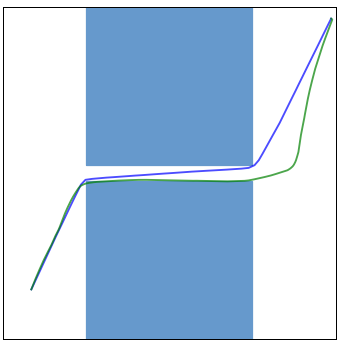
(a)

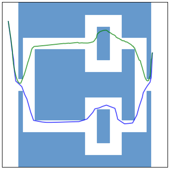
(b)

Figure 6: IL Experiment domains and results. The simple domain (a) and hard domain (b). A point robot should move only on the white free-space from a room on one side to the room on the other side while avoiding the blue obstacles. SGT plan (blue) executed successfully, sequential plan (green) collides with the obstacles.

We compare the sequential and Sub-Goal Tree (SGT) approaches for BC. Consider a point-robot motion-planning problem in a 2D world, with two obstacle scenarios termed simple and hard, as shown in Figure 6. In simple, the distribution of possible motions from left to right is uni-modal, while in hard, at least 4 modalities are possible.

For both scenarios we collected a set of 111K (100K train + 10K validation + 1K test) expert trajectories from random start and goal states using a state-of-the-art motion planner (OMPL’s(Şucan et al., 2012) Lazy Bi-directional KPIECE (Şucan & Kavraki, 2009) with one level of discretization). To account for different trajectory modalities, we chose a Mixture Density Network (MDN)(Bishop, 1994) as the parametric distribution of the predicted next state, both for the sequential and the SGT representations. We train the MDN by maximizing likelihood using Adam (Kingma & Ba, 2014). To ensure the same model capacity for both representations, we used the same network architecture, and both representations were trained and tested with the same data. Since the dynamical system is Markovian, the current and goal states are sufficient for predicting the next state in the plan, so we truncated the state history in the sequential model’s input to contain only the current state.

For simple, the MDNs had a uni-modal multivariate-Gaussian distribution, while for hard, we experimented with 2 and 4 modal multivariate-Gaussian distributions, denoted as hard-2G, and hard-4G, respectively. As we later show in our results the SGT representation captures the demonstrated distribution well even in the hard-2G scenario, by modelling a bi-modal sub-goal distribution.

We evaluate the models using unseen start-goal pairs taken from the test set. To generate a trajectory, we predict sub-goals, and connect them using linear interpolation. We call a trajectory successful if it does not collide with an obstacle en-route to the goal. For a failed trajectory, we further measure the severity of collision by the percentage of the trajectory being in collision.

Table 3 summarizes the results for both representations. The SGT representation is superior in all three evaluation criteria - motion planning success rate, trajectory prediction times (total time in seconds for the 1K trajectory predictions), and severity. Upon closer look at the two hard scenarios, the Sub Goal Tree with a bi-modal MDN outperforms sequential with 4-modal MDN, suggesting that the SGT trajectory decomposition better accounts for multi-modal trajectories.

	Success Rate		Prediction Times (Seconds)		Severity
	Sequential	SGT	Sequential	SGT	Sequential	SGT
Simple	0.541	0.946	487.179	28.641	0.0327	0.0381
Hard - 2G	0.013	0.266	811.523	52.22	0.0803	0.0666
Hard - 4G	0.011	0.247	1052.62	53.539	0.0779	0.0362

Table 3: Results for IL experiments.

Appendix E Technical Details for NMP Experiments Section 6.2

In this appendix we provide the full technical details of our policy gradient experiments presented in Section 6.2. We start by providing the explicit formulation of the NMP environment. We further provide a sequential-baseline not presented in the main text and its NMP environment and experimental results related to this baseline. We also present another challenging scenario – poles, and the results of SGT-PG and SeqSG in it. Finally, we conclude with modeling-related technical details .

E.1 Neural Motion Planning Formulation

In Section 6.2, we investigated the performance of SGT-PG and SeqSG executed in a NMP problem for the 7DoF Franka Panda robotic arm. That NMP formulation, denoted here as with-reset, allows for independent evaluations of motion segments, a requirement for FD-MSGT. The state $s\in\mathbb{R}^{9}$ describes the robot’s 7 joint angles and 2 gripper positions, normalized to $[-1,1]$. The models, SGT-PG and SeqSG, are tasked with predicting the states (sub-goals) in the plan.

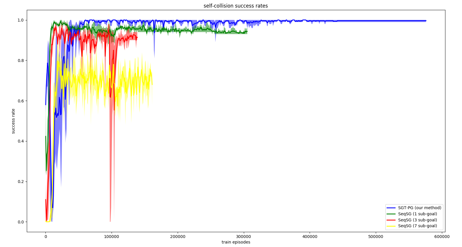
Figure 9: Success rates over training episodes of the self-collision scenario.

A segment $(s,s^{\prime})$ is evaluated by running a PID controller tracking a linear joint motion from $s$ to $s^{\prime}$. Let $s_{PID}$ denote the state after the PID controller was executed, and let $\alpha_{free}$ and $\alpha_{collision}$ be hyperparameters. We next define a cost function that encourages shorter paths, and discourages collisions; if a collision occurred during the PID execution, or 5000 simulation steps were not enough to reach $s^{\prime}$, a cost of $\alpha_{free}\cdot||s-s_{PID}||_{2}+\alpha_{collision}\cdot||s^{\prime}-s_{PID}||_{2}$ is returned. Otherwise, the motion was successful, and the segment cost is $\alpha_{free}\cdot||s-s^{\prime}||_{2}$. In our experiments we set $\alpha_{free}=1$ and $\alpha_{collision}=100$. Figures 9 and  10 show the training curves for the self-collision and wall scenarios respectively.

E.2 The SeqAction Baseline

We also evaluated a sequential baseline we denoted as SeqAction, which is more similar to classical RL approaches. Instead of predicting the next state, SeqAction predicts the next action to take (specifically the joint angles difference), and a position controller is executed for a single time-step instead of the PID controller of the previous methods.

SeqAction operates on a finite-horizon MDP (with horizon of $T=5000$ steps). We follow the sequential NMP formulation of Jurgenson & Tamar (2019); the agent gets a high cost on collisions, high reward when reaching close to the goal, or a small cost otherwise (to encourage shorter paths). We denote this NMP variant no-reset as segments are evaluated sequentially, without resetting the state between evaluations. To make the problem easier, after executing an action in no-reset, the velocity of all the links is manually set to 0.

Similarly to Jurgenson & Tamar (2019), we found that sequential RL agents are hard to train for neural motion planning with varying start and goal positions without any prior knowledge or inductive bias. We trained SeqAction in the self-collision scenario using PPO (Schulman et al., 2017), and although we achieved 100% success rate when fixing both the start and the goal (to all zeros and all ones respectively), the model was only able to obtain less than 0.1 success rate when varying the goal state, and showed no signs of learning when varying both the start and the goal.

E.3 The poles Scenario

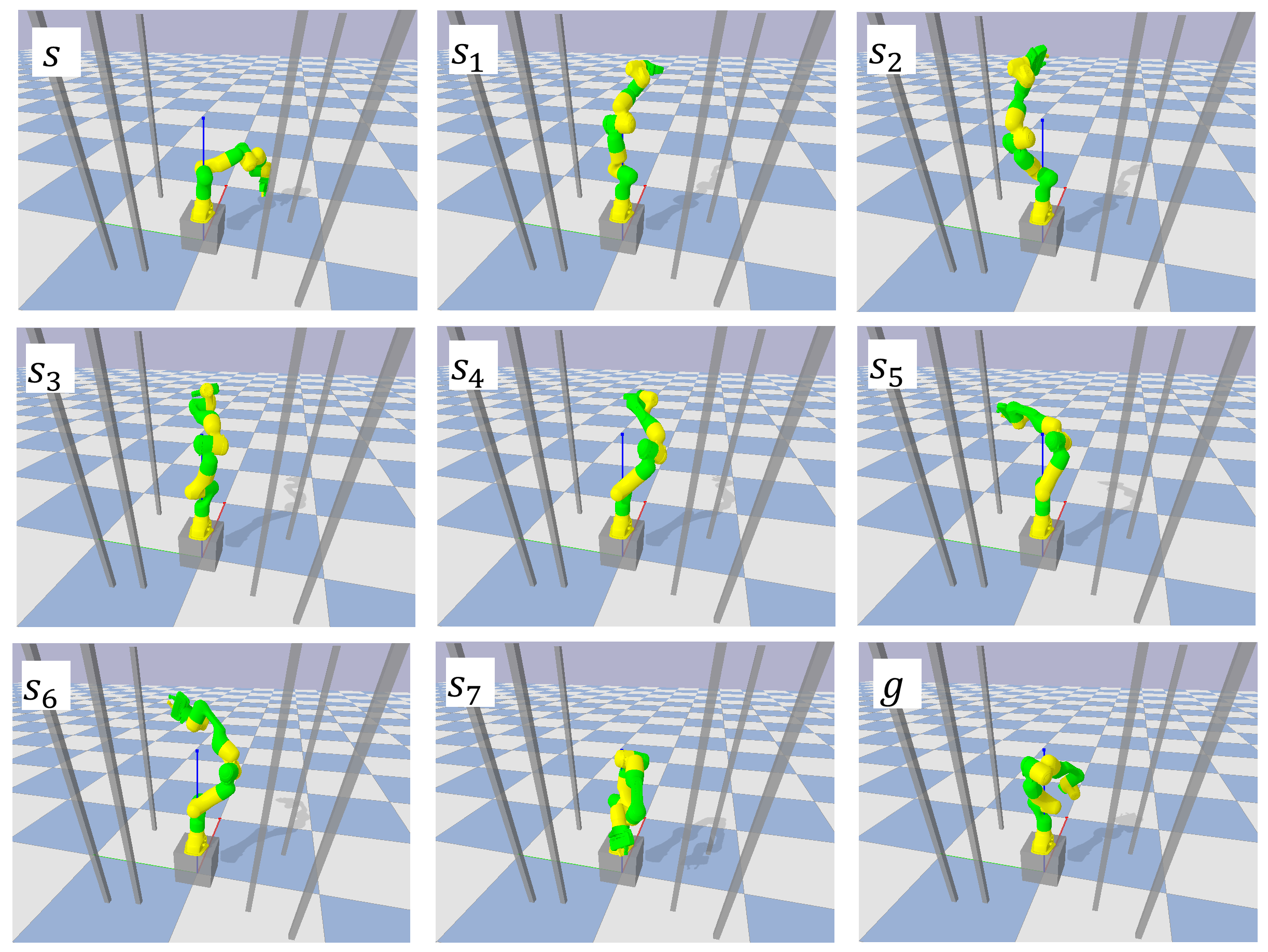
Figure 7: Robot trajectory poles scenario predicted with SGT-PG with 7 sub-goals. Top left start state, bottom right goal state. Notice that the two final segments $s_{6}$ to $s_{7}$ and $s_{7}$ to $g$ are longer than the rest, but are made possible by the robot getting into position in state $s_{6}$. Note that SGT-PG failed to find a trajectory for this $(s,g)$ pair with less sub-goals, indicating the hardness of the path.

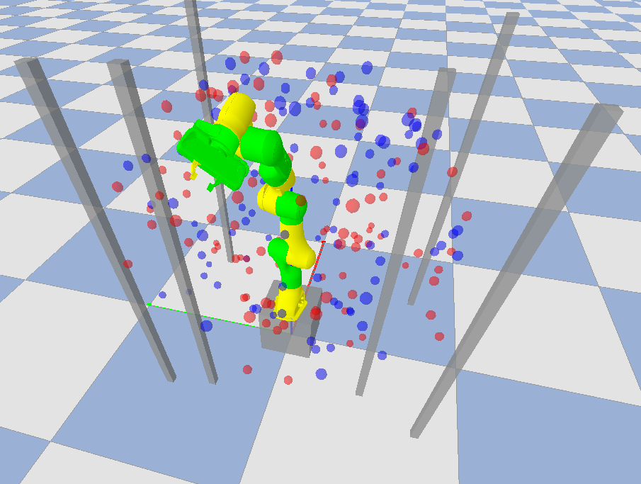
Figure 8: Start (blue) and goal (red) states in the test set of the poles scenario. Note that the agents are not exposed to these particular states during training.

model	# Sub-goals	Success rate
SGT-PG	1	0.646$\pm$0.053
	3	0.663$\pm$0.153
	7	0.696$\pm$0.116
SeqSG	1	0.616$\pm$0.013
	3	0.576$\pm$0.013
	7	0.49$\pm$0.02

Table 4: Success rate on the NMP poles scenario

We tested both SGT-PG and SeqSG on another scenario we call poles where the goal is to navigate the robot between poles as shown in Figures 7 and 8. Similar to the previous scenarios, Table 4 shows the success rates of both models for 1, 3, and 7 sub-goals. Again, we notice that SGT-PG attains much better results and improves as more sub-goals are added, while the performance of SeqSG deteriorates. Moreover, even for a single sub-goal, SGT-PG obtains better success rates compared to SeqSG. The high range displayed by SGT-PG is due to one random seed that obtained significantly lower scores.

E.4 Neural Network Architecture and Training Procedure

We next provide full technical details regarding the architecture and training procedure of SGT-PG and SeqSG described in Section 6.2.

Architecture and training of SGT-PG: The start and goal states, $s$ and $g$, are fed to a neural network with 3 hidden-layers of 20 neurons each and tanh activations. The network learns a multivariate Gaussian-distribution over the predicted sub-goal with a diagonal covariance matrix. Since the covariance matrix is diagonal, the size of the output layer is $18=2\cdot 9$, 9 elements learn the bias, and 9 learn the standard deviation in each direction. To predict the bias, a value of $\frac{s+g}{2}$ is added to the prediction of the network. To obtain the final standard deviation, we add two additional elements to the standard deviation predicted by the neural network : (1) a small value (0.05), to prevent learning too narrow distributions, and (2) a learnable coefficient in each of the directions that depends on the distance between $s$ and $g$, which allows large segments to predict a wider spread of sub-goals. These two changes were incorporated in order to mitigate log-likelihood evaluation issues.

SGT-PG trains on 30 $(s,g)$ pairs per training cycle, using the Adam optimizer (Kingma & Ba, 2014) with a learning rate of 0.005 on the PPO objective (Schulman et al., 2017) augmented with a max-entropy loss term with coefficient 1, and a PPO trust region of $\epsilon=0.2$. As mentioned in Section 5.2, when training level $d$ for a single $(s,g)$ pair, we sample $M$ sub-goals (in our experiments $M=10$) from the multivariate Gaussian described above, take the mean predictions of policies of depth $d-1$ and lower, and take the mean of costs as a $(s,g)$-dependent baseline. The repetition allows us to obtain a stable baseline without incorporating another learnable module – a value function. We found this method to be more stable than training on 300 different start-goal pairs (no repetitions). During test time we always take the mean prediction generated by the policies.

Architecture of SeqSG: This model has two components, a policy and a value function. The policy architecture is identical to that of SGT-PG. Note that only a single policy is maintained as the optimal policy is independent of the remaining horizon. We also found that learning the covaraince matrix causes stability issues for the algorithm, so the multivariate Gaussian only learns a bias term. The value function of SeqSG has 3 layers with 20 neurons each, and Elu activations. It predicts a single scalar which approximates $V(s,g)$, and is used as a state-dependent baseline to reduce the variance of the gradient estimation during training.

In order to compare apples-to-apples, SeqSG also trains on 30 $(s,g)$ pairs with 10 repetitions each. We trained the policy with the PPO objective (Schulman et al., 2017) with trust region of $\epsilon=0.05$. We used the Adam optimizer (Kingma & Ba, 2014), with learning rate of $0.005$ but we clipped the gradient with L2 norm of 10 to stabilize training. The value function is trained to predict the value with mean-squared error loss. We also trained it with Adam with a learning rate of $0.005$ but clipped the gradient L2 norm to 100.

We note that finding stable parameters for SeqSG was more challenging than for SGT-PG, as apparent by the gradient clippings, the lower trust region value, and our failure to learn the mutivariate Gaussian distribution covariance matrix.

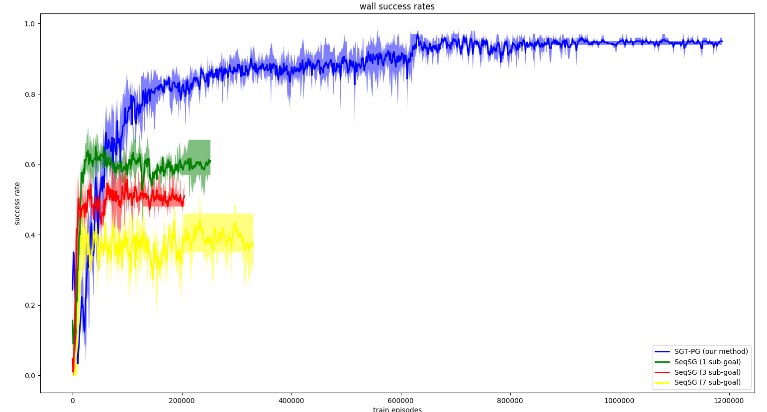
Figure 10: Success rates over training episodes of the wall scenario.

References

- Andrychowicz et al. (2017) Andrychowicz, M., Wolski, F., Ray, A., Schneider, J., Fong, R., Welinder, P., McGrew, B., Tobin, J., Abbeel, O. P., and Zaremba, W. Hindsight experience replay. In Advances in Neural Information Processing Systems, pp. 5048–5058, 2017.
- Bellemare et al. (2013) Bellemare, M. G., Naddaf, Y., Veness, J., and Bowling, M. The arcade learning environment: An evaluation platform for general agents. Journal of Artificial Intelligence Research, 47:253–279, 2013.
- Bertsekas (2005) Bertsekas, D. Dynamic programming and optimal control: Volume II. 2005.
- Bertsekas & Tsitsiklis (1996) Bertsekas, D. P. and Tsitsiklis, J. N. Neuro-dynamic programming. Athena Scientific, 1996.
- Bishop (1994) Bishop, C. M. Mixture density networks. Technical report, Citeseer, 1994.
- Chan (2010) Chan, T. M. More algorithms for all-pairs shortest paths in weighted graphs. SIAM Journal on Computing, 39(5):2075–2089, 2010.
- Deisenroth et al. (2013) Deisenroth, M. P., Neumann, G., Peters, J., et al. A survey on policy search for robotics. Foundations and Trends® in Robotics, 2(1–2):1–142, 2013.
- Dhiman et al. (2018) Dhiman, V., Banerjee, S., Siskind, J. M., and Corso, J. J. Floyd-warshall reinforcement learning learning from past experiences to reach new goals. arXiv preprint arXiv:1809.09318, 2018.
- Duan et al. (2016) Duan, Y., Chen, X., Houthooft, R., Schulman, J., and Abbeel, P. Benchmarking deep reinforcement learning for continuous control. In International Conference on Machine Learning, pp. 1329–1338, 2016.
- Ernst et al. (2005) Ernst, D., Geurts, P., and Wehenkel, L. Tree-based batch mode reinforcement learning. Journal of Machine Learning Research, 6(Apr):503–556, 2005.
- Floyd (1962) Floyd, R. W. Algorithm 97: shortest path. Communications of the ACM, 5(6):345, 1962.
- Fruit et al. (2017) Fruit, R., Pirotta, M., Lazaric, A., and Brunskill, E. Regret minimization in mdps with options without prior knowledge. In Advances in Neural Information Processing Systems, pp. 3166–3176, 2017.
- Ginsberg (1989) Ginsberg, M. L. Universal planning: An (almost) universally bad idea. AI magazine, 10(4):40–40, 1989.
- Greensmith et al. (2004) Greensmith, E., Bartlett, P. L., and Baxter, J. Variance reduction techniques for gradient estimates in reinforcement learning. Journal of Machine Learning Research, 5(Nov):1471–1530, 2004.
- Gu et al. (2017) Gu, S., Holly, E., Lillicrap, T., and Levine, S. Deep reinforcement learning for robotic manipulation with asynchronous off-policy updates. In 2017 IEEE international conference on robotics and automation (ICRA), pp. 3389–3396. IEEE, 2017.
- Ijspeert et al. (2013) Ijspeert, A. J., Nakanishi, J., Hoffmann, H., Pastor, P., and Schaal, S. Dynamical movement primitives: learning attractor models for motor behaviors. Neural computation, 25(2):328–373, 2013.
- Jayaraman et al. (2019) Jayaraman, D., Ebert, F., Efros, A. A., and Levine, S. Time-agnostic prediction: Predicting predictable video frames. In ICLR, 2019.
- Jurgenson & Tamar (2019) Jurgenson, T. and Tamar, A. Harnessing reinforcement learning for neural motion planning. In Robotics: Science and Systems (RSS), 2019.
- Kaelbling (1988) Kaelbling, L. P. Goals as parallel program specifications. In AAAI, volume 88, pp. 60–65, 1988.
- Kaelbling (1993) Kaelbling, L. P. Learning to achieve goals. In IJCAI, pp. 1094–1099. Citeseer, 1993.
- Kalashnikov et al. (2018) Kalashnikov, D., Irpan, A., Pastor, P., Ibarz, J., Herzog, A., Jang, E., Quillen, D., Holly, E., Kalakrishnan, M., Vanhoucke, V., et al. Qt-opt: Scalable deep reinforcement learning for vision-based robotic manipulation. arXiv preprint arXiv:1806.10293, 2018.
- Kingma & Ba (2014) Kingma, D. P. and Ba, J. Adam: A method for stochastic optimization. arXiv preprint arXiv:1412.6980, 2014.
- Kober et al. (2013) Kober, J., Bagnell, J. A., and Peters, J. Reinforcement learning in robotics: A survey. The International Journal of Robotics Research, 32(11):1238–1274, 2013.
- Konidaris et al. (2012) Konidaris, G., Kuindersma, S., Grupen, R., and Barto, A. Robot learning from demonstration by constructing skill trees. The International Journal of Robotics Research, 31(3):360–375, 2012.
- LaValle (2006) LaValle, S. M. Planning algorithms. Cambridge university press, 2006.
- Mann & Mannor (2014) Mann, T. and Mannor, S. Scaling up approximate value iteration with options: Better policies with fewer iterations. In International conference on machine learning, pp. 127–135, 2014.
- McGovern & Barto (2001) McGovern, A. and Barto, A. G. Automatic discovery of subgoals in reinforcement learning using diverse density. 2001.
- Menache et al. (2002) Menache, I., Mannor, S., and Shimkin, N. Q-cut—dynamic discovery of sub-goals in reinforcement learning. In European Conference on Machine Learning, pp. 295–306. Springer, 2002.
- Mishra et al. (2017) Mishra, N., Abbeel, P., and Mordatch, I. Prediction and control with temporal segment models. In Proceedings of the 34th International Conference on Machine Learning-Volume 70, pp. 2459–2468. JMLR. org, 2017.
- Mülling et al. (2013) Mülling, K., Kober, J., Kroemer, O., and Peters, J. Learning to select and generalize striking movements in robot table tennis. The International Journal of Robotics Research, 32(3):263–279, 2013.
- Munos & Szepesvári (2008) Munos, R. and Szepesvári, C. Finite-time bounds for fitted value iteration. Journal of Machine Learning Research, 9(May):815–857, 2008.
- Peters & Schaal (2008) Peters, J. and Schaal, S. Reinforcement learning of motor skills with policy gradients. Neural networks, 21(4):682–697, 2008.
- Pomerleau (1989) Pomerleau, D. A. ALVINN: An autonomous land vehicle in a neural network. In NIPS, pp. 305–313, 1989.
- Qureshi et al. (2018) Qureshi, A. H., Bency, M. J., and Yip, M. C. Motion planning networks. arXiv preprint arXiv:1806.05767, 2018.
- Riedmiller (2005) Riedmiller, M. Neural fitted q iteration–first experiences with a data efficient neural reinforcement learning method. In European Conference on Machine Learning, pp. 317–328. Springer, 2005.
- Ross et al. (2011) Ross, S., Gordon, G., and Bagnell, D. A reduction of imitation learning and structured prediction to no-regret online learning. In Proceedings of the fourteenth international conference on artificial intelligence and statistics, pp. 627–635, 2011.
- Russell & Norvig (2010) Russell, S. J. and Norvig, P. Artificial Intelligence - A Modern Approach (3. internat. ed.). Pearson Education, 2010.
- Schaul et al. (2015) Schaul, T., Horgan, D., Gregor, K., and Silver, D. Universal value function approximators. In International conference on machine learning, pp. 1312–1320, 2015.
- Schoppers (1989) Schoppers, M. J. Representation and automatic synthesis of reaction plans. PhD thesis, University of Illinois at Urbana-Champaign, 1989.
- Schulman et al. (2015) Schulman, J., Levine, S., Abbeel, P., Jordan, M., and Moritz, P. Trust region policy optimization. In International conference on machine learning, pp. 1889–1897, 2015.
- Schulman et al. (2017) Schulman, J., Wolski, F., Dhariwal, P., Radford, A., and Klimov, O. Proximal policy optimization algorithms. arXiv preprint arXiv:1707.06347, 2017.
- Şucan & Kavraki (2009) Şucan, I. A. and Kavraki, L. E. Kinodynamic motion planning by interior-exterior cell exploration. In Algorithmic Foundation of Robotics VIII, pp. 449–464. Springer, 2009.
- Şucan et al. (2012) Şucan, I. A., Moll, M., and Kavraki, L. E. The Open Motion Planning Library. IEEE Robotics & Automation Magazine, 19(4):72–82, December 2012. doi: 10.1109/MRA.2012.2205651. http://ompl.kavrakilab.org.
- Sung et al. (2018) Sung, J., Jin, S. H., and Saxena, A. Robobarista: Object part based transfer of manipulation trajectories from crowd-sourcing in 3d pointclouds. In Robotics Research, pp. 701–720. Springer, 2018.
- Sutton et al. (1999) Sutton, R. S., Precup, D., and Singh, S. Between mdps and semi-mdps: A framework for temporal abstraction in reinforcement learning. Artificial intelligence, 112(1-2):181–211, 1999.
- Sutton et al. (2000) Sutton, R. S., McAllester, D. A., Singh, S. P., and Mansour, Y. Policy gradient methods for reinforcement learning with function approximation. In Advances in neural information processing systems, pp. 1057–1063, 2000.
- Thorup & Zwick (2005) Thorup, M. and Zwick, U. Approximate distance oracles. Journal of the ACM (JACM), 52(1):1–24, 2005.
- Tsitsiklis & Van Roy (2001) Tsitsiklis, J. N. and Van Roy, B. Regression methods for pricing complex american-style options. IEEE Transactions on Neural Networks, 12(4):694–703, 2001.
- Williams (2014) Williams, R. Faster all-pairs shortest paths via circuit complexity. In Proceedings of the forty-sixth annual ACM symposium on Theory of computing, pp. 664–673, 2014.
- Zhang et al. (2018) Zhang, H., Heiden, E., Julian, R., He, Z., Lim, J. J., and Sukhatme, G. S. Auto-conditioned recurrent mixture density networks for complex trajectory generation. arXiv preprint arXiv:1810.00146, 2018.