Visualizing Strange Metallic Correlations in the 2D Fermi-Hubbard Model with AI

Abstract

Strongly correlated phases of matter are often described in terms of straightforward electronic patterns. This has so far been the basis for studying the Fermi-Hubbard model realized with ultracold atoms. Here, we show that artificial intelligence (AI) can provide an unbiased alternative to this paradigm for phases with subtle, or even unknown, patterns. Long- and short-range spin correlations spontaneously emerge in filters of a convolutional neural network trained on snapshots of single atomic species. In the less well-understood strange metallic phase of the model, we find that a more complex network trained on snapshots of local moments produces an effective order parameter for the non-Fermi-liquid behavior. Our technique can be employed to characterize correlations unique to other phases with no obvious order parameters or signatures in projective measurements, and has implications for science discovery through AI beyond strongly correlated systems.

I Introduction

Strongly correlated phases of matter are often described in terms of relatively simple real space order parameters, which are theoretically understood using Landau symmetry-breaking theory Wen (2004). For instance, ferromagnetism on a square lattice involves a uniform arrangement where the electrons' spins align and create a magnetic state with a wavevector ${\bf q=0}$. Antiferromagnetism, slightly more complex, is revealed by a ${\bf q}=$ $\pi$ alternation of the electrons' spin state on two sublattices. These choices, and incommensurate (spiral) order which bridges them at general ${\bf q}$, can be characterized in a unified way through the magnetic structure factor, $S({\bf q})$, and further generalized to include time-domain patterns via the dynamic susceptibility, $\chi({\bf q},\omega)$. Similar statements apply to charge density wave and other phases involving diagonal long-range order.

While many of our theoretical and experimental probes of interacting quantum systems have been constructed with coupling to these patterns in mind, there is an increasing realization that the most interesting strongly correlated phases might not be immediately accessible via such observables. Cuprate and iron pnictide superconductors, which combine closely entwined conventional phases with well-established order parameters, and much less well-understood non-Fermi liquid (NFL) or pseudogap phases with so far ``hidden orders" are examples Orenstein and Millis (2000); Varma et al. (2002); Sachdev and Chowdhury (2016), as is the zoo of orbital ferromagnetism, superconductivity, and Mott insulating behavior in twisted bilayer graphene Cao et al. (2018a, b). The community of strongly correlated quantum systems is thus faced with the challenge of developing new means of identifying complex phases.

Here, we introduce an unbiased approach in which artificial intelligence (AI) is used to extract hidden features from raw images of quantum many-body systems. We test our approach using projective measurements on a two-dimensional (2D) Fermi-Hubbard model, obtained through quantum gas microscopy of ultracold fermionic atoms in an optical lattice. We find that filters of a convolutional neural network (CNN), trained to recognize snapshots of fermions, capture features at different densities that have clear interpretation in terms of short- and long-range magnetic correlations. We further show that a more complex CNN can produce an effective order parameter for the NFL phase, based on the interplay of multiple types of density fluctuations, reflecting the more enigmatic nature of the correlations in this phase.

In the experiment, the 2D Fermi-Hubbard model is realized using a spin-balanced mixture of the first and third lowest energy states of ⁶Li loaded into a square optical lattice. We work at a magnetic field of 615 G in the vicinity of the Feshbach resonance near 690 G, which gives a scattering length of 1056(10)$\mathrm{a_{0}}$, where $\mathrm{a_{0}}$ is the Bohr radius The lattice depth is $7.25(2)E_{R}$, where $E_{R}$ is the lattice recoil energy and $E_{R}/h=14.66$ kHz. For these parameters we obtain $t/h=850(20)$ Hz and $U/t=8.0(1)$. Here, $t$ and $U$ are the nearest-neighbor hopping matrix element and the strength of onsite repulsive interaction, respectively, in the Hubbard model (see Appendix A).

Using quantum gas microscopy techniques Brown et al. (2017), we image the atoms in the lattice with single site resolution with a fidelity of 98%. When a fluorescence image is taken, atoms on doubly occupied sites undergo light-assisted collisions and appear empty. An image taken this way allows us to extract the local moment on each site. Alternatively, we can apply a short pulse of resonant light prior to taking an image to eject atoms of one of the two hyperfine states. This allows us to measure the single component density of the remaining hyperfine state.

Our lattice beams produce a harmonic trapping potential, which if uncompensated leads to significant variations of the local density. To study regions of uniform density, we flatten the potential using light shaped using a spatial light modulator Brown et al. (2019). In the subsequent analysis, we work with a flattened region of $20\times 20$ lattice sites.

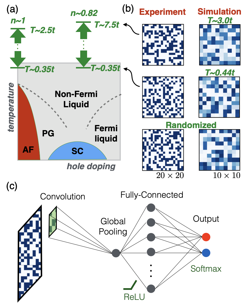
Figure 1: Phase diagram, sample snapshots, and CNN architecture. (a) Schematic phase diagram of cuprate high-temperature superconductors in the space of temperature and hole doping. AF, PG and SC stand for antiferromagnetic, pseudogap, and superconducting phases, respectively. (b) Sample experimental (left) and determinant quantum Monte Carlo (right) snapshots taken for $U=8t$ at the density $n\sim 0.82$ at different temperatures. The bottom row shows the lower-temperature snapshots whose pixels have been randomly shuffled, i.e., ``fake" snapshots. (c) The main convolutional neural network architecture used in this study. It contains a convolutional layer with one filter and one feature map followed by a global pooling layer, a hidden layer with eight fully connected neurons, and an output softmax layer with two neurons, each associated with a temperature limit. We use the rectified linear unit (ReLU) as the activation function in all but the output layer. In our experiments we observe that the presence of the fully connected layer accelerates the training of the neural network.

Figure 1 shows two randomly chosen samples of binarized occupancy snapshots at an average density of $n=0.82(2)$ at two extreme temperatures of $T\sim U\sim 8\,t$ and $T\sim 0.35\,t$. These parameters place us within the NFL region of a typical cuprate phase diagram [see Fig. 1(a)]. Thermometry is performed using averages of various correlation functions taken over such snapshots Brown et al. (2019).

$n=\to$	$0.97$	$0.835$	$0.82$	$0.735$	$0.70$	$0.64$	$0.58$
Spin-up/spin-down	$402$		$216$
Singles	$201$	$281$	$5023$	$290$	$342$	$281$	$330$

Table 1: Number of available experimental snapshots at $T\sim 0.35$ for different densities.

The increasingly large number of snapshots taken in quantum gas microscope experiments in various regions of the parameter space lends itself to data-driven approaches for science discovery, such as the enlisting of AI (see Table I for the number of snapshots used in this study). In fact, early implementations of machine learning techniques for the study of quantum many-body systems demonstrated great potential Carleo and Troyer (2017); Carrasquilla and Melko (2017); Ch'ng et al. (2017); Deng et al. (2017); van Nieuwenburg et al. (2017); Zhang and Kim (2017); Zhang et al. (2018). Recent applications to experimental data have directly led to the discovery of new physics Zhang et al. (2019); Bohrdt et al. (2019); Rem et al. (2019); Torlai et al. (2019); Samarakoon et al. (2020), modeling of their distribution Casert et al. , or the optimization of experimental processes Wigley et al. (2016); Picard et al. (2019), including those related to quantum gas microscopy.

CNNs offer an ideal platform for the detection of patterns in the experimental snapshots. Not only can they efficiently compress the information in images and use them for classification, but also their trained filters provide a window into the relevant features observed Zeiler and Fergus (2014). Figure 1(c) shows the main CNN architecture we have used. After labeling them according to their temperature, hundreds of snapshots taken at the extreme temperatures along with their labels are provided to the CNN for training. During the training, the network adjusts its free parameters to minimize the difference between given labels and its prediction (see Appendix B). The convolutional layer in our CNN interacts directly with the input snapshots and, therefore, examining the filter after the completion of training can teach us about the most important feature the network has picked up.

II Results

Figure 2(a) shows a sample $5\times 5$ filter for a CNN that is trained to distinguish experimental snapshots of a single species of fermions at the highest temperature ($T\sim 2.5t$) from those at the lowest temperature ($T\sim 0.35t$) when $n\sim 1$. If we expect mostly random behavior at high temperature, of the same order as the largest energy scale in the system, the features that spontaneously develop in the filters during training will most likely represent patterns found in the low-temperature snapshots. We find that the CNN consistently makes the distinction with more than 91% accuracy, and it does so using filters showing a distinctive pattern indicative of long-range antiferromagnetic (AF) correlations.

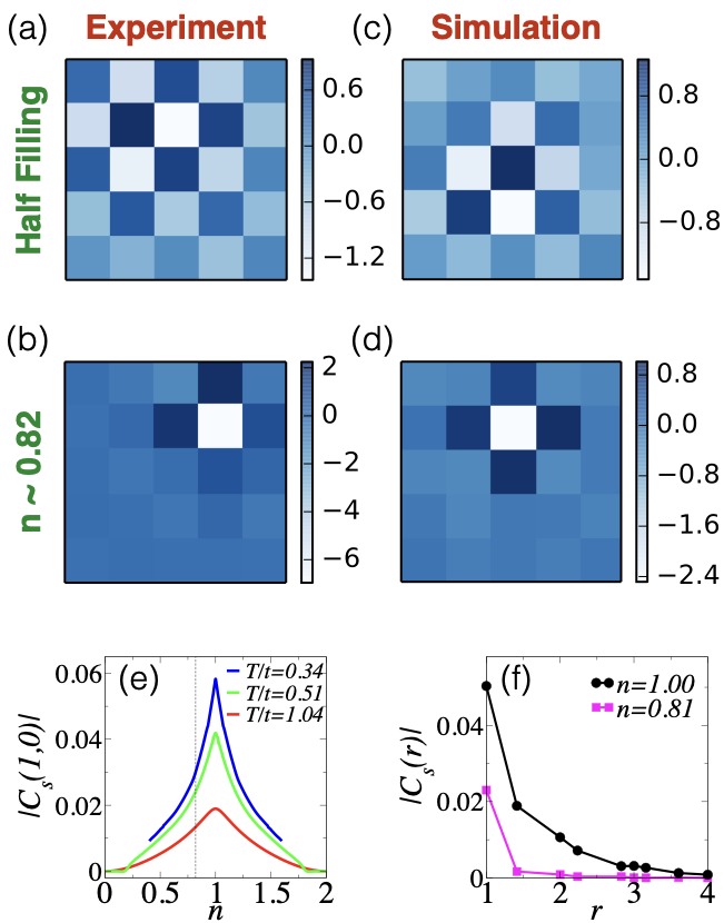
Figure 2: Analysis of single-species snapshots using CNNs with one filter. Sample $5\times 5$ trained filters for (a) $n\sim 1$ and (b) $n=0.82$. The CNN architecture is shown in Fig. 1(c). The testing accuracies are between 91% and 96%. The visual pattern in (a) is consistent with recognizing long-range antiferromagnetic (AF) order near half filling. The filter in (b) indicates a pattern capturing short-range AF correlations. (c, d) Similar sample filters evolved from training runs using determinant quantum Monte Carlo (DQMC) simulations at $T=0.1t$ and $0.44t$, with testing accuracies of 91% and 68%, respectively. (e, f) Theory data for the nearest-neighbor spin-spin correlation for $U=8t$ vs density at different temperatures (numerical linked cluster expansion), and vs distance for $n=0.81$ and $n=1.00$ at $T=0.44t$ (DQMC). These results illustrate that AI can capture the correct trends in magnetic behavior of the Hubbard model, and that the trained filters carry a clear physical interpretation.

Training the CNN using similar snapshots obtained for $n=0.82$ at $T\sim 7.5t$ and $0.35t$ results in filters that reflect a shorter-range anticorrelation between neighboring fermions of the same species [see Fig. 2(b)]. The nearest-neighbor checkerboard pattern emerging in the filters is consistent with the fact that the correlation length in the NFL region is about one lattice spacing Tranquada (2007). We find that this feature appears at different locations in the filter for different training runs, which points to a redundancy: on average the filter must reflect the translational symmetry of the underlying system. These findings suggest that the network effectively uses the strength of AF correlations as a measure for classifying snapshots of a single species of fermions. Figures 2(e) and  2(f) show that the density, distance, and temperature dependence of the magnetic correlations of the model, $C_{s}({\bf r})$ (see Appendix A), which are calculated here on a $10\times 10$ cluster using the determinant quantum Monte Carlo (DQMC) method Blankenbecler et al. (1981), or in the thermodynamic limit using the numerical linked cluster expansion (NLCE) Rigol et al. (2006); Khatami and Rigol (2011), support this observation.

Quantum Monte Carlo simulations also provide a platform to corroborate these findings. However, except in one spatial dimension, these simulations cannot provide projective measurements in the density basis. Instead, theory ``snapshots" can be constructed via expectation values of local charge or spin density using instances of auxiliary field variables during a simulation; for example, the $i$th pixel of a spin-up DQMC snapshot is $\left<\hat{n}_{i\uparrow}\right>_{h}=1-\mathscr{G}_{ii\uparrow}(h)$, where $\mathscr{G}_{ii\uparrow}(h)$ is the $i$th diagonal element of the spin-up equal time Green's function matrix for the auxiliary field instance $h$. We perform the simulations for a $10\times 10$ site Hubbard system with $U=8t$ at several average densities and temperatures (see Appendix D).

At high temperatures, of the order of $3t$, we find that density snapshots are fuzzy with no clear empty sites; mostly fluctuations about an average background density can be seen. This fuzziness is less of a concern for single-species snapshots [see Fig. 1(b)], although they too lose their pixelated character at higher temperatures. For this reason, to eliminate fuzziness as an obvious feature for the CNN to learn, instead of high-temperature snapshots, we use low-temperature images whose pixels have been randomly shuffled, effectively destroying any physical correlations. In the following, we refer to the latter as fake (as opposed to real) snapshots.

Figures 2(c) and 2(d) show sample filters from training experiments using theory snapshots of single species at half filling and $n=0.82$. Despite reduced accuracies of about 68% for the latter, which we believe is due to the exacerbation of the issue with the nonprojective nature of simulated images at this density, we find that the trained features are in excellent agreement with those obtained with quantum gas microscope snapshots. Together, they demonstrate that relevant spin correlations can be captured in an unbiased fashion through CNNs.

Studies of the origin of the NFL behavior, a central question in any theory of high-temperature superconductivity Sachdev (2010), have for decades been focused on its possible connections to the order parameter fluctuations of a magnetic quantum critical point Hertz (1976); Sachdev and Ye (1992); Millis (1993); Stewart (2001); Löhneysen et al. (2007); Sachdev (2010); Fitzpatrick et al. (2013). Here, we are in a position to ask whether any such fluctuations manifest themselves in charge correlations too, and to what extent they can be inferred from the other type of snapshots available in the experiment, those of local moments.

A similar analysis using images at the two extreme temperatures, however, is largely affected by the abundance of doubly occupied sites at $T\sim 7.5t$, and their lack of representation in the snapshots of local moments. Upon lowering the temperature to $T\sim 0.35t$, the fraction of doubly occupied sites at 18% doping reduces roughly by a factor of 4, from 12% to about 3% Khatami and Rigol (2011), providing the CNN again with an obvious feature with which to perform classification. Removing this bias by randomly populating pixels to create ``fake" replacements for high-temperature snapshots in the training, brings the accuracy down dramatically when $n=0.82$.

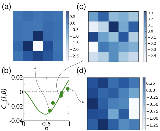
Figure 3: Analysis of local moment snapshots using CNNs with one filter. Representative $5\times 5$ filters for runs at (a) $n=0.58$, (c) $n=0.82$, and (d) $n=0.97$ using the same CNN architecture as one used for snapshots of single species. (b) The nearest-neighbor local moment correlation function from DQMC (solid line) on an $8\times 8$ cluster at $T=0.3t$ and from the experiment (circles) at similar low temperatures. The testing accuracy reaches (a) $89\%$, (c) $62\%$, and (d) $60\%$.

Figure 3 shows that the accuracy of CNNs trained on snapshots of local moments largely depends on the strength of short-range correlations between the moments. The largest accuracies (almost $90\%$) are typically achieved near quarter filling, where the correlations are the most negative. Patterns observed in filters trained in this region are also consistent with the anticorrelation of neighboring moments [Fig. 3(a)]. The accuracy drops to around $60\%$ at $n=0.82$, near the zero crossing of the correlator, which is shown in Fig. 3(b). Typical trained filters do not display any immediately recognizable patterns either [see Fig. 3(c)]. Near half filling, the correlations between local moments are positive due to the bunching of holes and doubly occupied sites Cheuk et al. (2016). Here, we find that despite the relatively low accuracies ($\lesssim 65\%$), trained filters often do reflect the bunching of empty sites [Fig. 3(d)].

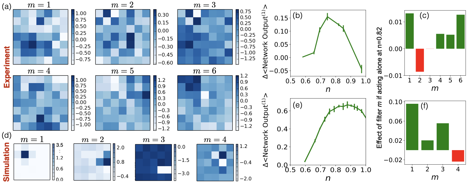
Figure 4: Analysis of local moment snapshots using CNNs with multiple filters. (a) The six filters of a trained CNN. Training is performed with the 5023 experimental local moment snapshots taken at $n=0.82$ and $T\sim 0.35$. The testing accuracy remains at $62\%$ with less than $1\%$ variation over the last 20 epochs (see Appendix B). (b) The difference in the average network output for $T\sim 0.35t$ real and fake snapshots as a function of the density when all six filters are present: $\Delta\left<\text{Network Output}^{(1)}\right>\equiv\left<\text{Network Output}^{(1)}({\bf X}^{\text{real}})\right>-\left<\text{Network Output}^{(1)}({\bf X}^{\text{fake}})\right>$. Superscript $(1)$ indicates the value at the output neuron responsible for real low-temperature snapshots (see Appendix B). This quantity indicates roughly the percentage of the output attributable to factors other than the density. (c) Similar to (b) at $n=0.82$ when the CNN has access to one filter at a time. (d) Four representative filters of a CNN with sixteen $5\times 5$ filters trained using DQMC snapshots of local moments (see Appendix D). (e, f) Same as (b) and (c), but obtained using the CNN in (d).

The comparison of Fig. 3(c) ($n=0.82$) with Figs. 3(a) and  3(d) ($n=0.58,0.97$) makes it clear that snapshots of local moments in the NFL region of the Hubbard model do not contain a single dominant ordering pattern and that a more advanced treatment may be necessary to capture the physics. In Fig. 4, we show results of a training with a CNN, modified to include six $7\times 7$ filters in its convolutional layer (see Appendix B). The bigger data set we have available for snapshots of local moments at this density allows us to experiment with different filter sizes and numbers of filters. We find that including more than one filter in the CNN improves the best accuracies only marginally in this case, up to around 65%, and having too many and/or much larger filters can still result in overfitting. We also find that using a deeper CNN with two convolutional layers does not significantly improve the accuracy.

Figure 4(a) shows six filters of a sample CNN trained on the local moment snapshots. Their fuzzy patterns offer some insight into possible spatial arrangements of local moments at low temperatures. As we see below, patterns in filters $m=1,4,5$, and $6$ are more frequently associated by the network with real low-temperature snapshots at this filling, whereas patterns in filter $m=2$ are more frequently associated with fake snapshots.

By transferring the knowledge of the CNN to other densities, we find that the network is the most sensitive to correlations around the NFL region. Figure 4(b) shows the difference in probabilities that a snapshot and its fake counterpart are categorized as belonging to the NFL region, effectively eliminating density itself as a factor in the signal. We find this quantity to be maximal in the vicinity of $n=0.8$, suggesting that the CNN as a whole is in fact focusing on local moment correlations more unique to the NFL region and slightly lower densities.

While the contribution of individual filters to the CNN's decision making cannot be completely isolated, we can study what the network output would be if each filter were to act alone (see Appendix B). Figure 4(c) shows this quantity averaged over samples at $n=0.82$, after subtracting the value for the corresponding fake snapshot, for each of the six filters shown in Fig. 4(a). The results suggest that filters 1 and 6, if acting alone, would have the largest effect on the decision making at this average density, followed by filters 2, 4, and 5, while filter 3 plays almost no role at all. The negative value for filter 2 indicates that the network signal is larger on average for fake snapshots in that case.

Using DQMC, we verify that similar trends can be observed in simulated snapshots of local moments. However, unlike with the experimental snapshots, here, we find that the accuracy generally increases with increasing the number of filters in the CNN, while increasing the filter size does not necessarily improve the performance. We attribute these to the fundamental difference between the two types of snapshots (projective vs nonprojective). Figure 4(d) highlights a representative sample of $5\times 5$ filters of a CNN with 16 such filters, trained on simulated snapshots reaching to an accuracy of 87% (see Appendix C). They appear to measure a variety of short-range correlations to assist the network in making decisions. Figure 4(e) shows the overall signal of the CNN for correlations unique to the NFL phase, plotted across densities. It has a broad peak around the NFL region. As shown in Fig. 4(f), patterns in the first three filters seem to be mostly associated with real snapshots in the NFL region, while the pattern in the $m=4$ filter is mostly associated with the fake snapshots. We find that including the information about doubly occupied sites, i.e., using full density snapshots, generally improves the diversity of features seen in the trained filters while yielding the same basic trends.

III Discussion

Using specially designed artificial neural networks, we have developed algorithms for extracting organizing patterns of correlated particles from raw quantum many-body data in an unbiased fashion and without any prior theoretical knowledge. When applied to the snapshots of one of the two species of fermionic atoms in a 2D optical lattice, our approach yields patterns indicative of long- and short-range AF correlation near and away from the commensurate filling, consistent with theory. We show that these features can be reproduced using nonprojective measurements from DQMC simulations.

Our analysis provides a window into the signatures of the NFL phase, one of the most mysterious and theoretically challenging phases in correlated electron systems, in snapshots of local moments from the quantum gas microscope. We show that in this case, a more complex neural network can be constructed and trained to be sensitive to correlations specific to the strange metallic phase. A similar analysis of snapshots with information about both species of particles in future experiments Koepsell et al. (2020) may further reveal the interplay between spin and charge fluctuations in this region.

Nonlinearities in the neural network model make the interpretation of features seen in the filters vis-à-vis correlations in the physical snapshots challenging since the knowledge of the network can be divided in nontrivial ways among its different components. An early example of this was the surprisingly successful classification of snapshots of the Ising lattice gauge theory at $T=0$ and $T=\infty$, despite the lack of an order parameter, using CNNs with multiple filters Carrasquilla and Melko (2017). The procedure we have introduced here overcomes aspects of this challenge. We point out that the nonlinearities are key for the success of our CNNs; for example, the principal component analysis Jolliffe (2002), a linear unsupervised learning method, largely fails to draw any meaningful distinction between sets of snapshots (see Appendix E).

The techniques developed in this work for the AI-assisted feature extraction in projective measurements can be adapted to peek into other mysterious phenomena for the Fermi-Hubbard model, such as the pseudogap phase Chiu et al. (2019), or the magnetic polaron which has been observed closer to half filling Koepsell et al. (2019). They can also be employed to study other microscopic models of correlated systems. Our work paves the way for AI-related studies that go beyond mere categorization and the quest for gaining more predictive power and focus instead on the inner workings of the machines to advance our understanding of complicated natural phenomena.

Appendix A The Fermi-Hubbard Model

The Hamiltonian for the 2D Fermi-Hubbard model in particle-hole symmetric form is expressed as

$$\hat{H} = -t\sum_{\left<{\bf i},{\bf j}\right>\,\sigma}\left(\hat{c}^{\dagger}_{\bf i\,\sigma}\hat{c}^{\phantom{\dagger}}_{\bf j\,\sigma}+\text{H.c.}\right)$$

$$+ U\sum_{\bf i}\left(\hat{n}_{{\bf i}\uparrow}-\frac{1}{2}\right)\left(\hat{n}_{{\bf i}\downarrow}-\frac{1}{2}\right)$$

$$- \mu\sum_{\bf i}(\hat{n}_{\bf i\uparrow}+\hat{n}_{\bf i\downarrow}),$$

where $\hat{c}^{\dagger}_{{\bf i}\sigma}$ ($\hat{c}^{\phantom{\dagger}}_{{\bf i}\sigma}$) creates (annihilates) a fermion with spin $\sigma$ on site ${\bf i}$, and $\hat{n}_{{\bf i}\sigma}=\hat{c}^{\dagger}_{{\bf i}\sigma}\hat{c}^{\phantom{\dagger}}_{{\bf i}\sigma}$ is the number operator. $\left<{\bf i},{\bf j}\right>$ denotes nearest neighbors on a square lattice, $U=8t$ is the strength of the onsite repulsive interaction in the numerical simulations, and $\mu$ is the chemical potential. $\mu=0$ corresponds to half filling, although density fluctuations around half filling exist in our grand canonical ensemble. $t=1$ (also $\hbar=1$ and $k_{B}=1$) sets the energy scale. The spin correlation function is calculated as $C_{s}({\bf r})=\left<\hat{S}_{z,{\bf i}}\hat{S}_{z,{\bf i+r}}\right>$, where $\hat{S}_{z,{\bf i}}=\frac{1}{2}(\hat{n}_{{\bf i}\uparrow}-\hat{n}_{{\bf i}\downarrow})$ and $\left<\dots\right>$ denotes the expectation value. The local moment correlation function is calculated as $C_{m}({\bf r})=\left<\hat{m}^{2}_{z,{\bf i}}\ \hat{m}^{2}_{z,{\bf i+r}}\right>$, where $\hat{m}^{2}_{z,{\bf i}}=(\hat{n}_{{\bf i}\uparrow}-\hat{n}_{{\bf i}\downarrow})^{2}$.

Appendix B Training the Convolutional Neural Network

We implement our CNNs using TENSORFLOW ten . The minimalistic design in Fig. 1(c) we have adopted reflects the need to reduce the number of free parameters to avoid overfitting given the sizes of our data sets. To train, we assign a label, $Y$, to each snapshot based on the temperature at which it is taken, or whether it is real or fake. Each label is stored in the one-hot format, i.e., a binary array of two numbers, one of which is 1 and the other 0. The index for 1 indicates the category (high or low temperature, or real or fake) to which each snapshot belongs. Given an input image ${\bf X}$, the value arriving at the first of the two output neurons of the CNN shown in Fig. 1(c), e.g., at the neuron we have associated in our labels to the low-temperature (or real) snapshots, is

$$O_{1}^{out}({\bf X})=\sum_{h}O_{h}^{hid}({\bf X})\times W_{h}^{out\ (1)}+b^{out\ (1)},$$ (2)

where the sum is over hidden neurons,

$$O_{h}^{hid}({\bf X}) = \textrm{ReLU}\left(\left[\frac{1}{N_{s}}\sum_{stride:s}\textrm{ReLU}\left({\bf W}^{filter}\cdot{\bf X}(s)+b^{filter}\right)\right]\times W_{h}^{hid}+b^{hid}_{h}\right),$$ (3)

$N_{s}$ is the number of strides the filter takes around the image convolving with different sections, ${\bf W}^{filter}$ is the matrix of pixel values for the filter, ${\bf X}(s)$ is the matrix of pixel values for the section of the image the filter is convolving with in stride $s$, ReLU is the rectified linear unit activation function, and $b^{filter}$, $W_{h}^{hid}$, $b^{hid}_{h}$, $W_{h}^{out(1)}$, and $b^{out(1)}$ are numbers representing other weights and biases in the network. $O_{1}^{out}$, along with the value arriving at the second output layer $O_{2}^{out}({\bf X})$, are then passed through the softmax activation function to obtain two probabilities as network outputs:

$$[ \textrm{Network Output}^{(1)}({\bf X}),\ \textrm{Network Output}^{(2)}({\bf X})]$$ (4)

$$= \textrm{softmax}[O_{1}^{out}({\bf X}),\ O^{out}_{2}({\bf X})].$$

The input snapshot is classified as belonging to category $i$ if $O^{net}_{i}$ is the higher probability, where $O^{net}_{i}=\textrm{Network Output}^{(i)}$ for brevity. The accuracy is defined as the percentage of correct classifications given known labels $Y$. The convolution of the trained filter with sections of the input image as it moves around in strides of one in every direction creates a ``feature map" in which large overlaps between patterns in the filter and the image are highlighted.

For training, we use the Adam optimizer, which is an extension of stochastic gradient descent, to minimize the cross-entropy cost function, defined as

$$c= - \frac{1}{N_{d}}\sum_{\bf X}\sum_{i=1}^{2}(Y_{i}({\bf X})\ln[O^{net}_{i}({\bf X})]$$

$$+ [1-Y_{i}({\bf X})]\ln[1-O^{net}_{i}({\bf X})]),$$

where $N_{d}$ is the number of data. During the training, we keep between 10% and 20% of the snapshots from the CNN and use them to perform unbiased testing of the accuracy.

B.1 CNN with more than one filter

In cases where we have more than one filter in the convolutional layer, we have modified the architecture to have no fully connected hidden layer in order to reduce the total number of network parameters; the output of each filter after pooling is instead fully connected to the output layer. The value arriving at the output neuron that is responsible for firing when a real snapshot ${\bf X}$ is provided to the input, $O_{1}^{out}({\bf X})$, can then be expressed as a linear combination of contributions from individual filters:

$$O_{1}^{out}({\bf X}) = \sum_{m=1}^{N_{f}}F_{m}^{(1)}({\bf X}),$$ (6)

$$F_{m}^{(1)}({\bf X}) = \left[\frac{1}{N_{s}}\sum_{stride:s}\textrm{ReLU}\left({\bf W}_{m}^{filter}\cdot{\bf X}(s)+b_{m}^{filter}\right)\times W_{m}^{out(1)}\right]+\frac{b^{out(1)}}{N_{f}},$$ (7)

where $N_{f}$ is the number of filters, and $W_{m}^{out(1)}$ and $b_{m}^{filter}$ are again numbers representing other weights and biases in the network. As in the case of the CNN with one filter, the network output is obtained using Eq. (4).

B.2 Effect of individual filters

To estimate the effect of filter $m$ on the outcome, we replace $O^{(1,2)}({\bf X})$ with $F_{m}^{(1,2)}({\bf X})$ before the softmax function,

$$[ \textrm{Network Output}_{m}^{(1)}({\bf X}),\textrm{Network Output}_{m}^{(2)}({\bf X})]$$ (8)

$$= \textrm{softmax}[F_{m}^{(1)}({\bf X}),F_{m}^{(2)}({\bf X})],$$

so that we can interpret $\left[\textrm{Network Output}_{m}^{(1)}({\bf X}^{real})-\textrm{Network Output}_{m}^{(1)}({\bf X}^{fake})\right]$ as the percentage the network output for ${\bf X}$, based on the action of filter $m$ alone, has to do with factors other than the density itself.

B.3 Augmentation of data

We augment Shorten and Khoshgoftaar (2019) our data for the experimental single-species snapshots before training [Figs. 2(a) and  2(b)] by applying point-group symmetries of the square lattice to each snapshot. This will increase the data by a factor of 8, and in these cases, helps make the training smoother and/or faster. However, we find that generally, such augmentation of data, or breaking the $20\times 20$ images into smaller subregions, does not significantly affect the final accuracy. This is consistent with the fact that the network architectures we have used in this work are not deep and do not show serious overfitting even before the data augmentation.

B.4 Training Progression

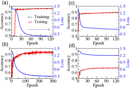
Figure 5: Progression of CNN accuracy during training with single-species snapshots. (a) Training and unbiased testing accuracies, along with the value of the loss function when using experimental snapshots at $n\sim 1$ to train the CNN with one filter, leading to the filter shown in Fig. 2(a). (b-d) Same as (a), but for trainings leading to filters in Figs. 2(b)-2(d). DQMC snapshots are used in (c) and (d). (a) and (c) correspond to trainings near half filling and (b) and (d) correspond to trainings at $n=0.82$.

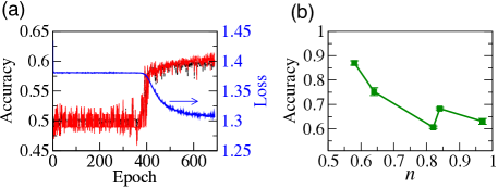
Figure 6: Progression of CNN accuracy during training with local moment snapshots. (a) Same as Fig. 5(a), but for the training with snapshots of local moments at $n=0.82$ leading to the filter shown in Fig. 3(c). (b) The average of maximum testing accuracies, obtained through four or five separate trainings, vs density.

To monitor the training progression and look for signs of overfitting, especially in the case of CNNs with more than one filter, we track the training and the unbiased testing accuracies as well as the loss function, defined in Eq. (B), over epochs. An epoch is when the network has gone over the entire data set once.

Figure 5 shows the results for various trainings using single-species snapshots that lead to filters presented in Fig. 2. In each case, we stop the training roughly when the loss function reaches a plateau. As can be seen, the training and the unbiased testing accuracies, which agree throughout the training process, also settle to their maxima.

Figure 6(a) shows similar results for the sample training with snapshots of local moments that lead to the filter presented in Fig. 3(c). For this case, we find that it takes longer for any training to be achieved and that the fluctuations in the accuracies are larger. Figure 6(b) shows the average of maximum accuracies achieved through four or five different training runs with different random number seeds over the range of densities for which snapshots of local moments were available. We see that as the strength of local correlations decreases by increasing the density towards half filling [shown in Fig. 3(b)], the maximum accuracies we can achieve also generally decrease.

Figure 7 shows the same training progressions for the case of CNNs with multiple filters, trained on snapshots of local moments at $n=0.82$, leading to results shown in Fig. 4. Despite the deviation of the average of two accuracies from each other beyond $\sim 1000$ epochs when experimental snapshots are used [Fig. 7(a)], signaling the beginning of overfitting due to the relatively large number of free parameters in the CNN, large fluctuations in the accuracies cause overlapping of the two curves even after 5000 epochs. When DQMC snapshots are used, the signs of overfitting are observed only after increasing the number of $5\times 5$ filters to about 60.

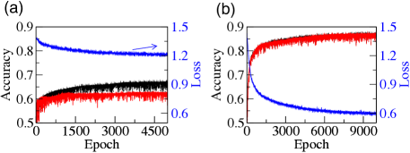
Figure 7: Progression of accuracy of CNNs with multiple filters during trainings with local moment snapshots. Same as Fig. 5, except that (a) experimental and (b) DQMC snapshots of local moments are used to train CNNs with 6 and 16 filters, showcased in Fig. 4.

Appendix C CNN with Sixteen Filters for Theory Snapshots of Local Moments

Figure 8 shows the result of training a CNN with 16 filters using 15000 $10\times 10$ theory snapshots of local moments. This is the same CNN whose filters are featured in Fig. 4(d). To obtain the snapshots in the DQMC approach, we note that for a particular auxiliary field, the expectation value of the local double occupancy reduces to its uncorrelated value; the product of the expectation values for spin-up and spin-down occupancies. Therefore, the local moment at site $i$ can be written as $\left<\hat{n}_{{\bf i}\uparrow}\right>+\left<\hat{n}_{{\bf i}\downarrow}\right>-2\left<\hat{n}_{{\bf i}\uparrow}\right>\left<\hat{n}_{{\bf i}\downarrow}\right>$.

Figure 8(a) shows the general improvement of the testing accuracy by increasing the number of filters. Figure 8(b) shows the 16 trained filters, which similarly to what we find for spin, point to only short-range fluctuations. One can find many redundancies. However, a few representative patterns [those features in Fig. 4(d)] emerge. Figure 8(c) shows the average network output when the network trained at $n=0.82$ is tested on configurations across a range of densities. We also test the network on fake snapshots. A nonmonotonic behavior emerges in both cases. Subtracting the average network output for the real and fake snapshots at each density results in a curve that has a broad peak around $n=0.85$ and showcases the extent of learned correlations between local moments in this CNN that have to do with factors other than the average density itself [Fig. 8(d)]. See Appendix B for more details.

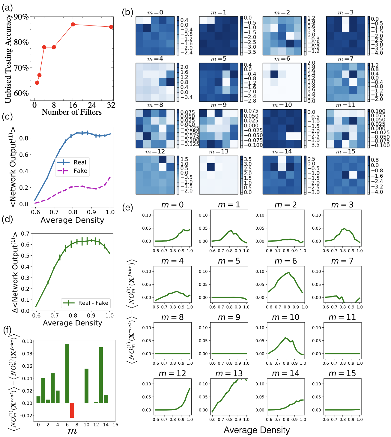
Figure 8: Analysis of DQMC local moment snapshots using a CNN with 16 filters. (a) The general improvement in the prediction accuracy of the CNN by increasing the number of filters. (b) Trained filters when $n=0.82$ and $T=0.44t$. Note that pixel values or their range in one filter should not be compared with those in other filters since a filter-dependent bias is added to the result of the convolution before it is passed through the ReLU activation function (see Appendix B). The testing accuracy is around $87\%$. (c) Average network output when a real or fake DQMC snapshot is provided as input, as a function of average density for this CNN. Here, 1 means all the snapshots are classified as likely to be real $n=0.82$ snapshots, 0 means all the snapshots are classified as likely to be fake $n=0.82$ snapshots, and 0.5 means neither of the two options is preferred. (d) The difference between the two curves in (c), representing the average percentage the decisions made by the CNN have to do with factors other than the density itself. (e) Similar to (d) when the CNN has access to one filter at a time (see Appendix B). (f) Same as in (e), but at $n=0.82$.

To attribute certain features seen in trained filters in Fig. 8(b) to correlations unique to the NFL region, we have to rule out their dominance at other densities. Figure 8(e) shows the performance of individual filters over the same range of densities we used to study the network output. Figure 8(f) further highlights the values in Fig. 8(e) at $n=0.82$. Based on these results, filters that significantly contribute to the CNN's decision-making process and are unique to the NFL phase and, therefore, are the best candidates for offering insight into local moment fluctuations are $m=1,3,6,7$, and $10$. The most frequently seen correlation seems to be the one between two neighboring empty sites. Filters $m=6$ and $13$ signal that the network also partly uses the information about the density gradient near local moments to make a decision.

Appendix D Determinantal Quantum Monte Carlo Snapshots

The implementation of DQMC used in the work proceeds via the exact rewriting of the interacting electron-electron problem as independent electrons moving in a space-imaginary time auxiliary field $h({\bf r},\tau)$. This reformulation involves first expressing the partition function ${\cal Z}$ for the original Hubbard Hamiltonian as a path integral, and then the use of a Hubbard-Stratonovich transformation to decouple the electrons. The original fermionic degrees of freedom are then traced out analytically, leaving an equivalent expression for ${\cal Z}$ as an integral over $h({\bf r},\tau)$. Detailed descriptions can be found in Refs. Blankenbecler et al. (1981); White et al. (1989); Assaad and Evertz (2008).

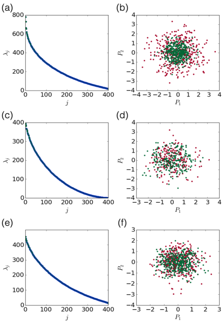
Figure 9: PCA of the experimental snapshots. (a, b) Eigenvalues of the covariance matrix of data for single-species snapshots at $n\sim 1$ and their projection to the space of the two largest principal components. The same 402 snapshots at each of the two extreme temperatures, used for Fig. 2, are also used here. Although the data points corresponding to the lower temperature [green (dark gray) circles in (b)] are slightly less spread out than their high temperature counterparts [red (light gray) circles in (b)], there is no obvious clustering of data based on temperature. (c, d) The same as (a) and (b), except for $n=0.82$ and that 216 available snapshots at each of the two extreme temperatures are used. (e, f) The same as (c) and (d), except that 400 real and 400 fake snapshots of local moments are used. No discernible patterns emerge in these projections either.

Here we focus on aspects of DQMC which have specific implications to the machine learning process. The most crucial is that, unlike world-line quantum Monte Carlo methods or cold-atom experiments, which directly sample the $0$ or $1$ occupation of sites ${\bf r}$ by the fermions, at any point (snapshot) in a DQMC simulation, the fermionic occupation is represented by a real number giving the probability of occupation of that site in the specific $h({\bf r},\tau)$ currently being sampled. As the temperature is lowered below $t$, sharper images containing pixels more closely resembling binary pixels in the experimental snapshots emerge. In fact, one can show that in the atomic limit, local expectation values approach step functions as $T\to 0$. This ``smearing" of the occupation makes some aspects of machine learning via these snapshots more challenging. However, whether individual snapshots present (0,1) fermion occupations or not, the strong correlation physics (magnetism, superconductivity, strange metallicity) of the Hubbard model needs to be built up from many thousands of snapshots. It is the task of uncovering these many-body effects that is shared by the theoretical and experimental images investigated here with AI.

The presence of the fermion ``sign problem" Loh et al. (1990); Troyer and Wiese (2005); Iglovikov et al. (2015) in DQMC simulations can complicate the interpretation of the theory snapshots. To avoid this complication to the extent possible, at $n=0.82$, we work at temperatures where the problem is not severe, where at least $90\%$ of the auxiliary field configurations have a positive sign. We also treat the network output during the testing process the same way we treat the expectation value of a conventional observable, $O$, by computing $\left<O\mathscr{S}\right>/\left<\mathscr{S}\right>$ in place of $\left<O\right>$, where $\mathscr{S}$ is the sign associated with the auxiliary field configuration resulting in a snapshot Ch'ng et al. (2017). Like the network output, $O$ is often a nonlinear function of the auxiliary field.

Appendix E Principal Component Analysis

We have employed the linear principal component analysis (PCA) Jolliffe (2002), an unsupervised learning algorithm, to perform dimensional reduction on the experimental data and examine whether any features emerge in the low-dimensional space, revealing any potential linear relation between pixels as an indicator for identifying low-temperature snapshots.

In the PCA, one forms a matrix of data, ${\bf x}$ by flattening the matrix of pixel values for each snapshot and placing them as an array of $400$ binary numbers in each row (of ${\bf x}$). In the next step, the covariance matrix of data is composed as ${\bf x}^{T}\cdot{\bf x}$. Diagonalizing the $400\times 400$ matrix, we obtain its eigenvalues, whose magnitudes are a measure for the variance of the data along the principal axes, determined by the corresponding eigenvectors. As demonstrated for the two-dimensional Ising model in a pioneering application in physics Wang (2016), a dominant eigenvalue is indicative of a clear distinguishing pattern in the snapshots that can be represented as a linear combination of its pixels (their projection to the corresponding principal axis).

Figure 9 shows our results for both single-species ($n\sim 1$ and $n=0.82$) and local moment ($n=0.82$) snapshots. The PCA does not seem to be able to draw any particular distinction between low and high temperature or real and fake snapshots in any of the cases as there are no clear signs of clustering of data points based on temperature or whether or not they correspond to real snapshots. Figures 9(a) and 9(b) show, respectively, the eigenvalues of the covariance matrix of data for snapshots of single species near half filling and their projections to the space formed by the first two principal axes, representing the directions of the largest variance in data. A large gap between the first few eigenvalues and the rest of them would indicate that there are clear linear indicators for distinguishing sets of data Wang (2016), something we do not observe here. This is also inferred from the projection of data in Fig. 9(b), where, other than a slightly larger spread of data points at the lower temperature, no clear separation between the hot and cold data points is formed in the space of the first two principal components. Figures 9(c)-9(f) show a similar trend for both the single species and local moment snapshots at $n=0.82$.

References

- Wen (2004) X. Wen, Quantum Field Theory of Many-Body Systems: From the Origin of Sound to an Origin of Light and Electrons, Oxford Graduate Texts (OUP Oxford, 2004).
- Orenstein and Millis (2000) J. Orenstein and A. J. Millis, Science 288, 468 (2000).
- Varma et al. (2002) C. Varma, Z. Nussinov, and W. van Saarloos, Physics Reports 361, 267 (2002).
- Sachdev and Chowdhury (2016) S. Sachdev and D. Chowdhury, Progress of Theoretical & Experimental Ph 2016 (2016).
- Cao et al. (2018a) Y. Cao, V. Fatemi, S. Fang, K. Watanabe, T. Taniguchi, E. Kaxiras, and P. Jarillo-Herrero, Nature 556, 43 (2018a).
- Cao et al. (2018b) Y. Cao, V. Fatemi, A. Demir, S. Fang, S. L. Tomarken, J. Y. Luo, J. D. Sanchez-Yamagishi, K. Watanabe, T. Taniguchi, E. Kaxiras, R. C. Ashoori, and P. Jarillo-Herrero, Nature 556, 80 (2018b).
- Brown et al. (2017) P. T. Brown, D. Mitra, E. Guardado-Sanchez, P. Schauß, S. S. Kondov, E. Khatami, T. Paiva, N. Trivedi, D. A. Huse, and W. S. Bakr, Science 357, 1385 (2017).
- Brown et al. (2019) P. T. Brown, D. Mitra, E. Guardado-Sanchez, R. Nourafkan, A. Reymbaut, C.-D. Hébert, S. Bergeron, A.-M. S. Tremblay, J. Kokalj, D. A. Huse, P. Schauß, and W. S. Bakr, Science 363, 379 (2019).
- Carleo and Troyer (2017) G. Carleo and M. Troyer, Science 355, 602 (2017).
- Carrasquilla and Melko (2017) J. Carrasquilla and R. G. Melko, Nat. Phys. 13, 431 (2017).
- Ch'ng et al. (2017) K. Ch'ng, J. Carrasquilla, R. G. Melko, and E. Khatami, Phys. Rev. X 7, 031038 (2017).
- Deng et al. (2017) D.-L. Deng, X. Li, and S. Das Sarma, Phys. Rev. B 96, 195145 (2017).
- van Nieuwenburg et al. (2017) E. P. L. van Nieuwenburg, Y.-H. Liu, and S. D. Huber, Nat. Phys. 13, 435 (2017), letter.
- Zhang and Kim (2017) Y. Zhang and E.-A. Kim, Phys. Rev. Lett. 118, 216401 (2017).
- Zhang et al. (2018) P. Zhang, H. Shen, and H. Zhai, Phys. Rev. Lett. 120, 066401 (2018).
- Zhang et al. (2019) Y. Zhang, A. Mesaros, K. Fujita, S. D. Edkins, M. H. Hamidian, K. Ch'ng, H. Eisaki, S. Uchida, J. C. S. Davis, E. Khatami, and E.-A. Kim, Nature 570, 484 (2019).
- Bohrdt et al. (2019) A. Bohrdt, C. S. Chiu, G. Ji, M. Xu, D. Greif, M. Greiner, E. Demler, F. Grusdt, and M. Knap, Nature Physics 15, 921 (2019).
- Rem et al. (2019) B. S. Rem, N. Käming, M. Tarnowski, L. Asteria, N. Fläschner, C. Becker, K. Sengstock, and C. Weitenberg, Nature Physics 15, 917 (2019).
- Torlai et al. (2019) G. Torlai, B. Timar, E. P. L. van Nieuwenburg, H. Levine, A. Omran, A. Keesling, H. Bernien, M. Greiner, V. Vuletić, M. D. Lukin, R. G. Melko, and M. Endres, Phys. Rev. Lett. 123, 230504 (2019).
- Samarakoon et al. (2020) A. M. Samarakoon, K. Barros, Y. W. Li, M. Eisenbach, Q. Zhang, F. Ye, V. Sharma, Z. L. Dun, H. Zhou, S. A. Grigera, C. D. Batista, and D. A. Tennant, Nature Communications 11, 892 (2020).
- (21) C. Casert, K. Mills, T. Vieijra, J. Ryckebusch, and I. Tamblyn, arXiv:2002.07055 [cond-mat.quant-gas] (2020).
- Wigley et al. (2016) P. B. Wigley, P. J. Everitt, A. van den Hengel, J. W. Bastian, M. A. Sooriyabandara, G. D. McDonald, K. S. Hardman, C. D. Quinlivan, P. Manju, C. C. N. Kuhn, I. R. Petersen, A. N. Luiten, J. J. Hope, N. P. Robins, and M. R. Hush, Scientific Reports 6, 25890 EP (2016).
- Picard et al. (2019) L. R. B. Picard, M. J. Mark, F. Ferlaino, and R. van Bijnen, Measurement Science and Technology 31, 025201 (2019).
- Zeiler and Fergus (2014) M. D. Zeiler and R. Fergus, in ``Visualizing and Understanding Convolutional Networks" in Computer Vision – ECCV 2014, edited by D. Fleet, T. Pajdla, B. Schiele, and T. Tuytelaars (Springer International Publishing, Cham, 2014) pp. 818–833.
- Tranquada (2007) J. Tranquada, in ``Neutron Scattering Studies of Antiferromagnetic Correlations in Cuprates", in Handbook of High-Temperature Superconductivity, edited by J. R. Schrieffer and J. Brooks (Springer, New York, NY, 2007).
- Blankenbecler et al. (1981) R. Blankenbecler, D. J. Scalapino, and R. L. Sugar, Phys. Rev. D 24, 2278 (1981).
- Rigol et al. (2006) M. Rigol, T. Bryant, and R. R. P. Singh, Phys. Rev. Lett. 97, 187202 (2006).
- Khatami and Rigol (2011) E. Khatami and M. Rigol, Phys. Rev. A 84, 053611 (2011).
- Sachdev (2010) S. Sachdev, Physica Status Solidi (b) 247, 537 (2010).
- Hertz (1976) J. A. Hertz, Phys. Rev. B 14, 1165 (1976).
- Sachdev and Ye (1992) S. Sachdev and J. Ye, Phys. Rev. Lett. 69, 2411 (1992).
- Millis (1993) A. J. Millis, Phys. Rev. B 48, 7183 (1993).
- Stewart (2001) G. R. Stewart, Rev. Mod. Phys. 73, 797 (2001).
- Löhneysen et al. (2007) H. v. Löhneysen, A. Rosch, M. Vojta, and P. Wölfle, Rev. Mod. Phys. 79, 1015 (2007).
- Fitzpatrick et al. (2013) A. L. Fitzpatrick, S. Kachru, J. Kaplan, and S. Raghu, Phys. Rev. B 88, 125116 (2013).
- Cheuk et al. (2016) L. W. Cheuk, M. A. Nichols, K. R. Lawrence, M. Okan, H. Zhang, E. Khatami, N. Trivedi, T. Paiva, M. Rigol, and M. W. Zwierlein, Science 353, 1260 (2016).
- Koepsell et al. (2020) J. Koepsell, S. Hirthe, D. Bourgund, P. Sompet, J. Vijayan, G. Salomon, C. Gross, and I. Bloch, Phys. Rev. Lett. 125, 010403 (2020).
- Jolliffe (2002) I. Jolliffe, Principal component analysis (John Wiley and Sons, Ltd, 2002).
- Chiu et al. (2019) C. S. Chiu, G. Ji, A. Bohrdt, M. Xu, M. Knap, E. Demler, F. Grusdt, M. Greiner, and D. Greif, Science 365, 251 (2019).
- Koepsell et al. (2019) J. Koepsell, J. Vijayan, P. Sompet, F. Grusdt, T. A. Hilker, E. Demler, G. Salomon, I. Bloch, and C. Gross, Nature 572, 358 (2019).
- (41) M. Abadi, et al., TensorFlow: Large-scale machine learning on heterogeneous systems (2015). Software available from tensorflow.org.
- Shorten and Khoshgoftaar (2019) C. Shorten and T. M. Khoshgoftaar, Journal of Big Data 6, 60 (2019).
- White et al. (1989) S. R. White, D. J. Scalapino, R. L. Sugar, E. Y. Loh, J. E. Gubernatis, and R. T. Scalettar, Phys. Rev. B 40, 506 (1989).
- Assaad and Evertz (2008) F. Assaad and H. Evertz, in ``World-line and Determinantal Quantum Monte Carlo Methods for Spins, Phonons and Electrons" in Computational Many-Particle Physics, edited by H. Fehske, R. Schneider, and A. Weiße (Springer Berlin Heidelberg, Berlin, Heidelberg, 2008) pp. 277–356.
- Loh et al. (1990) E. Y. Loh, J. E. Gubernatis, R. T. Scalettar, S. R. White, D. J. Scalapino, and R. L. Sugar, Phys. Rev. B 41, 9301 (1990).
- Troyer and Wiese (2005) M. Troyer and U.-J. Wiese, Phys. Rev. Lett. 94, 170201 (2005).
- Iglovikov et al. (2015) V. I. Iglovikov, E. Khatami, and R. T. Scalettar, Phys. Rev. B 92, 045110 (2015).
- Wang (2016) L. Wang, Phys. Rev. B 94, 195105 (2016).