Heterogeneous Graph Neural Networks
for Malicious Account Detection

Abstract.

We present, GEM, the first heterogeneous graph neural network approach for detecting malicious accounts at Alipay, one of the world’s leading mobile cashless payment platform. Our approach, inspired from a connected subgraph approach, adaptively learns discriminative embeddings from heterogeneous account-device graphs based on two fundamental weaknesses of attackers, i.e. device aggregation and activity aggregation. For the heterogeneous graph consists of various types of nodes, we propose an attention mechanism to learn the importance of different types of nodes, while using the sum operator for modeling the aggregation patterns of nodes in each type. Experiments show that our approaches consistently perform promising results compared with competitive methods over time.

1. Introduction

Large scale online services such as Gmail, Facebook and Alipay have becoming popular targets for cyber attacks. By creating malicious accounts, attackers can propagate spam messages, seek excessive profits, which are essentially harmful to the eco-systems. For example, numerous abused bot-accounts were used to send out billions of spam emails across the email system. What is more serious is that in financial systems like Alipay, once a large number of accounts be taken over by a malicious user or a group of them, those malicious users could possibly cash out and gain ill-gotten earnings, that enormously harms the whole financial system. Effectively and accurately detecting such malicious accounts plays an important role in such systems.

Many existing security mechanisms to deal with malicious accounts have extensively studied the attack characteristics  (Xie et al., 2008; Zhao et al., 2009; Huang et al., 2013; Cao et al., 2014; Stringhini et al., 2015) which hopefully can discern the normal and malicious accounts. To exploit such characteristics, existing research mainly spreads in three directions. First, Rule-based methods directly generate sophisticated rules for identification. For example, Xie et al. (Xie et al., 2008) proposed “spam payload” and “spam server traffic” properties for generating high quality regular expression signatures. Second, Graph-based methods reformulate the problem by considering the connectivities among accounts. This is based on the intuition that attackers can only evade individually but cannot control the interactions with normal accounts. For example, Zhao et al. (Zhao et al., 2009) analyzed connected subgraph components by constructing account-account graphs to identify large abnormal groups. Thrid, Machine learning-based methods learn statistic models by exploiting large amount of historical data. For examples, Huang et al. (Huang et al., 2013) extracted features based on graph properties and built supervised classifiers for identifying malicious account. Cao et al. (Cao et al., 2014) advanced the usages of aggregating behavioral patterns to uncover malicious accounts in an unsupervised machine learning framework.

As attacking strategies from potential adversaries change, it is crucial that a well-behaved system could adapt to the evolving strategies (Zhao et al., 2009; Cao et al., 2014). We summarize the following two major observations from attackers as the fundamental basis of our work. (1) Device aggregation. Attackers are subjected to cost on computing resources. That is, due to economic constraints, it is costly if attackers can control a large amount of computing resources. As a result, most accounts owned by one attacker or a group of attackers will signup or sigin frequently on only a small number of resources. (2) Activity aggregation. Attackers are subject to the limited time of campaigns. Basically, attackers are required to fulfil specific goals in a short term. That means the behaviors of malicious accounts controlled by a single attacker could burst in limited time.

The weaknesses of attackers have been extensively analyzed, however, it’s still challenging to identify attackers with both high precision and recall. In financial systems like Alipay, it is way important to accurately identify malicious account as many as possible. The reason is in two-folds: (1) The illegal behaviors like cash-out is essentially harmful to the whole financial system or even the national security; (2) As an Internet service company, we need to reduce the unnecessary disturbances and interruptions to normal users, i.e. providing friendly services. Existing methods (Zhao et al., 2009) usually achieve very low false positive rate (friendly services) by setting strict constraints but potentially missing out the opportunities on identifying much more suspicious accounts, i.e. with a high false negative rate. The reason is that the huge amount of benign accounts interwined with only a small number of suspicious accounts, and this results into a low signal-to-noise-ratio. It is quite common that normal accounts share the same IP address with malicious accounts due to the noisy data, or the IP address comes from a common proxy. Thus make it important to jointly consider the “Device aggregation” and “Activity aggregation” altogether in the view of heterogeneous graph consists of various types of devices such as phone number, Media access control address (MAC), IMEI (International Mobile Equipment Identity), SIM number, and so on.

In this work, we present, Graph Embeddings for Malicious accounts (GEM), a novel nueral network-based graph technique based on the literature of graph representation learning (Hamilton et al., 2017), which jointly considers “Device aggregation” and “Activity aggregation” in heterogeneous graphs. Our proposed approach essentially models the topology of the heterogeneous account-device graph, and simultaneously considers the characteristics of activities of the accounts in the local strucuture of this graph. The basic idea of our model is that whether a single account is normal or malicious is a function of how the other accounts “congregate” with this account via devices in the topology, and how those other accounts shared the same device with this account “behave” in timeseries. To allow various types of devices, we use attention mechanism to adaptively learn the importance of different types of devices. Unlike existing methods that one first studies the graph properties (Huang et al., 2013) or pairwise comparisons of account activities (Cao et al., 2014), then feeds into a machine learning framework, our proposed method directly learns a function for each account given the context of the local topology and other accounts’ activities nearby in an end to end way.

We deploy the proposed work as a real system at Alipay. It can detect tens of thousands malicious accounts daily. We empirically show that the experimental results significantly outperform the results from other competitive methods.

We summarize the contributions of this work as follows:

• We present a novel neural network based graph representation method for identifying malicious accounts by jointly capturing two of attackers’ weaknesses, summarized as “Device aggregation” and “Activity aggregation” in a heterogeneous graph. To our best knowledge, this is the first fraud detectoin problem addressed by graph neural network approaches with careful graph constructon.

• Our approach is deployed at Alipay, one of the largest third-party mobile and online cashless payment platform serving more than 4 hundreds of million users. The approach can detect tens of thousands malicious accounts daily.

2. Preliminaries

In this section, we first briefly present some preliminary contents of graph representation learning techniques recently developed.

2.1. Graph Neural Networks

The first class is concerned with predicting labels over a graph, its edges, or its nodes. Graph Neural Networks were introduced in Gori et al.(Gori et al., 2005) and Scarselli et al. (Scarselli et al., 2009) as a generalization of recursive neural networks that can directly deal with a more general class of graphs, e.g. cyclic, directed and undirected graphs.

Recently, generalizing convolutions to graphs have shown promising results (Bruna et al., 2013; Defferrard et al., 2016). For example, Kipf & Welling (Kipf and Welling, 2016) propose simple filters that operate in a 1-step neighborhood around each node. Assuming $X\in\mathbb{R}^{N,D}$ is a matrix of node features vectors $x_{i}\in\mathbb{R}^{D}$, an undirected graph $\mathcal{G}=(\mathcal{V},\mathcal{E})$ with $N$ nodes $v_{i}\in\mathcal{V}$, edges $(v_{i},v_{j})\in\mathcal{E}$, an adjacency matrix $A\in\mathbb{R}^{N\times N}$. They propose the following convolution layer:

(1) $$H^{(t+1)}=\sigma\bigg{(}\tilde{A}H^{(t)}W^{(t)}\bigg{)},$$

where $\tilde{A}$ is a symmetric normalization of $A$ with self-loops, i.e. $\tilde{A}=\hat{D}^{-\frac{1}{2}}\hat{A}\hat{D}^{-\frac{1}{2}}$, $\hat{A}=A+I$ and $\hat{D}$ is the diagonal node degree matrix of $\hat{A}$, $H^{(t)}$ denotes the $t$-th hidden layer with $H^{(0)}=X$, $W^{(t)}$ is the layer-specific parameters, and $\sigma$ denotes the activation functions. The GCN (Kipf and Welling, 2016) essentially learn a function $f(X,A)$ that helps the representation of each node $x_{i}$ by exploiting its neighborhood defined in $A$. By modeling nodes as documents, and edges as citation links, their algorithm achieves state-of-art results on tasks of classifying documents in citation networks like Citeseer, Cora, and Pubmed.

At the same time, a novel connection between graphical models and neural networks has been studied by Dai et al. (Dai et al., 2016). One key observation is that the solution of variational latent distribution $q_{i}(\mu_{i})$ for each node $i$ needs to satisfy the following fixed point equations:

(2) $$\log q_{i}(\mu_{i})=g(\mu_{i},x_{i},\{q_{j}\}_{j\in\mathcal{N}(i)}).$$

Moreover, Smola et al. (Smola et al., 2007) showed that there exists another feature space such that one can find an injective embedding $h_{i}$ as sufficient statistics corresponding to the original $q_{i}(\mu_{i})$ function. As a result, Dai et al. (Dai et al., 2016) shows that for any given above fixed point equation one can always find an equivalent transformation in another feature space:

(3) $$h_{i}=f(x_{i},\{h_{j}\}_{j\in\mathcal{N}(i)}).$$

As such, one can directly learn the graphical model in the embedding space $h$ and directly optimize the funtion $f$ by extra link functions in a neural network framework. Such representation is even more powerful compared with traditional graphical models where each variable is limited by a function from an exponential family.

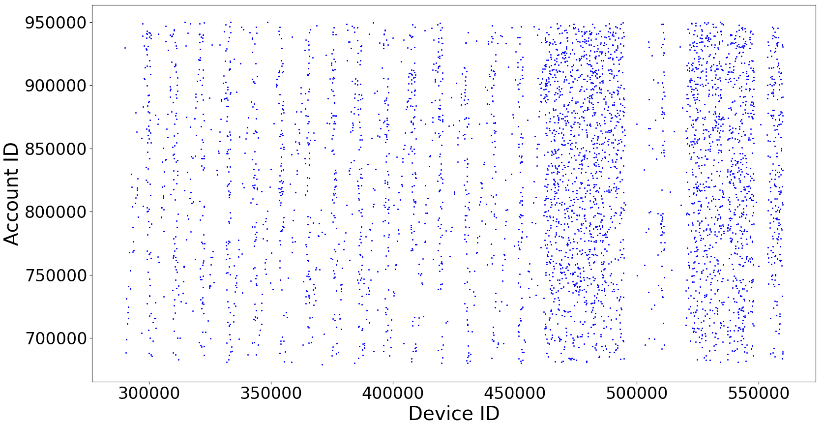
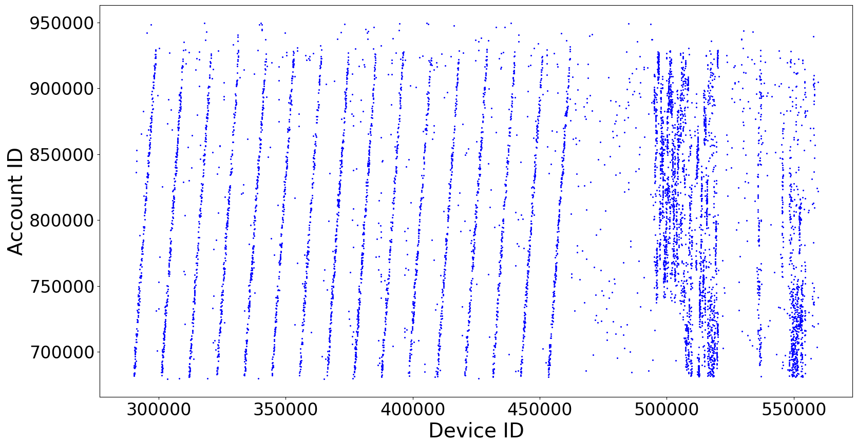
Figure 1. Device aggregation patterns: normal accounts (first) v.s. malicious accounts (second), malicious accounts tend to aggregate compared with normal accounts.

To summarize, the works in this domain essentially are built based on an iterative-style neighborhood aggregation method (Hamilton et al., 2017):

(4) $$h_{i}^{(t+1)}=f(x_{i},x_{j\in\mathcal{N}(i)},h_{i}^{(t)},h_{j\in\mathcal{N}(i)}^{(t)})$$

where $f(\cdot)$ is a parameterized non-linear transformation. Most of the efforts in this domain study the “receptive fields” (Liu et al., 2018) that aggregation operators should work on, because compared with data like images where each pixel have exactly 8 neighbors, the nodes in the graph domain can vary a lot.

More recently, Liu et al. (Liu et al., 2018) propose GeniePath, which aims to adaptively filter each node’s receptive fields, compared with GCN that does convolution on pre-defined receptive fields. And this yields much better results.

Our methods can be viewed as a variant of graph convolutional networks, that is, we design a approach that uses the sum operator to capture the “aggregation” patterns in each node’s $T$-step neighborhood, while using attention mechnisms to reweigh the importances of various types of nodes in the “heterogeneous” graph.

2.2. Node Embedding

The second class of techniques consists of graph embedding methods that aim to learn representation of each node while preserving the graph structure (Hamilton et al., 2017). They explicitly model the relationships among node pairs. For example, some methods directly use the adjacency matrix (Ahmed et al., 2013; Belkin and Niyogi, 2002), $t$-th order adjacency matrix (Cao et al., 2015), and others simulate random walks by approximating the high order adjacency matrix in a randomized manner (Grover and Leskovec, 2016; Perozzi et al., 2014).

Formally, most approaches aim to minimize an emprical loss, $\mathcal{L}$, over a set of training node pairs:

(5) $$\mathcal{L}=\sum_{(v_{i},v_{j})\in\mathcal{E}}\ell(f_{\mathrm{dec}}(f_{\mathrm{enc}}(v_{i}),f_{\mathrm{enc}}(v_{j})),f_{\mathcal{G}}(v_{i},v_{j})),$$

where $f_{\mathrm{enc}}:\mathcal{V}\mapsto\mathbb{R}^{k}$ is the encoder function, $f_{\mathrm{dec}}:\mathcal{V}\times\mathcal{V}\mapsto\mathbb{R}^{+}$ is the decoder function such as $f_{\mathrm{dec}}(z_{i},z_{j})=z_{i}^{\top}z_{j}$, and $f_{\mathcal{G}}(\cdot,\cdot)\mapsto\mathbb{R}^{+}$ is the so called pairwise proximity function, and $\ell:\mathbb{R}\times\mathbb{R}\mapsto\mathbb{R}$ is a specific loss function used to measure the reconstruction ability of $f_{\mathrm{dec}},f_{\mathrm{enc}}$ to a user-specified pairwise proximity measure $f_{\mathcal{G}}$.

The methods in this domain are unsupervised algorithms. They learn node embeddings on the graph without use of ground truth labels. Such node embeddings can be used as statistic properties of the graph as (Huang et al., 2013), and be fed into a classifier for final prediction.

Pratically the random walk-based proximity measure (Hamilton et al., 2017) has proven to achieve state-of-art results on many tasks like citation networks, protein networks etc. We will report the empirical results of such methods in experiments.

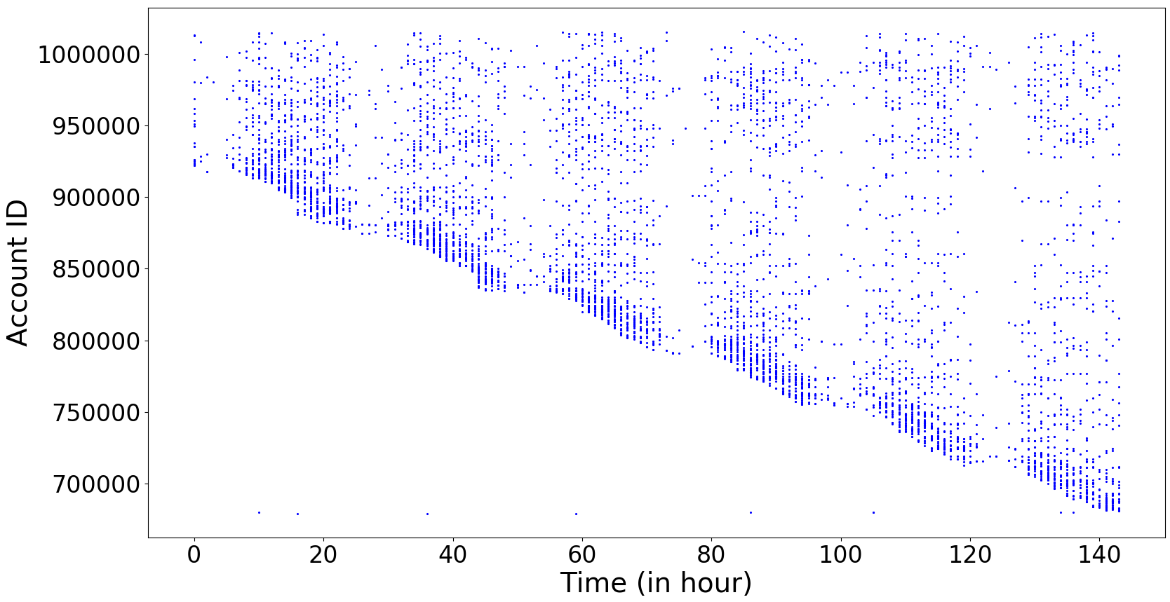
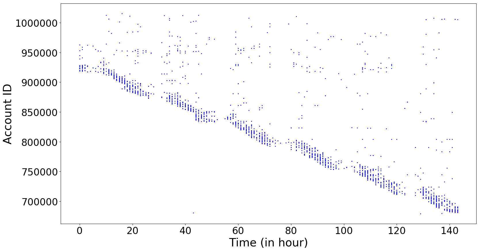
Figure 2. Activity aggregation patterns: normal accounts (first) v.s. malicious accounts (second), newly registered malicious accounts tend to be active only in a short term.

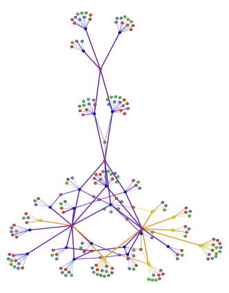
Figure 3. Visualization of one of connected subgraph component from our data, a total of 210 vertices consists of 20 normal accounts (Blue), 7 malicious accounts (Yellow), and rest of vertices correspond to 6 types of devices. The thicknesses of those edges denote the estimated attention coefficients will be discussed in section 4.3.4.

3. The Proposed Approaches

In this section, we first describe the patterns we found in the real data at Alipay, then discuss a motivated approach based on connected subgraph components. Inspired from this intuitive approach, we discuss the construction of a heterogeneous graph based on the characteristics of the real data, and finally present the approach on modeling malicious accounts.

3.1. Data Analysis

In this section we study the patterns of “Device aggregation” and “Activity aggregation” demonstrated by the real data at Alipay.

Device aggregation. The basic idea of device aggregation is that if an account signups or logins the same device or a common set of devices together with a large number of other accounts, then such accounts would be suspicious. One can simply calculate the size of the connnected subgraph components (Zhao et al., 2009) as a measure of risk for each account.

Activity aggregation. The basic idea of activity aggregation is that if accounts sharing the common devices behave in batches, then those accounts are suspicious. One can simply define the inner product of activities of two accounts sharing the same device as a measure of affinity, i.e. $S_{i,i^{\prime}}^{a}=\langle x_{i},x_{i^{\prime}}\rangle$. Apparently the consistent behaviors over time between account $i$ and $i^{\prime}$ mean high degrees of affinity. Such measures of affinity between two accounts can be further used to split a giant connected subgraph to improve the false positive rate (Zhao et al., 2009).

We illustrate such two patterns from the data of Alipay in Figure 1 and Figure 2. Figure 1 shows account-device graphs accumulated in 7 consecutive days. We do not differentiate the different types of device in this graph. A blue dot means the account has behaviors (signups or logins) associated with the corresponding device. For normal accounts, the blue dots uniformly scatter over the account-device graph, compared with malicious accounts, the blue dots show strong signals that the specific device could connect with huge number of accounts in various patterns. Figure 2 illustrates the behavior patterns of each account over time, where each blue dot denotes that there is an activity of account $i$ at time $t$. The behaviors of normal accounts in graph on the left show that each newly registered normal accounts behave evenly in the next several days, whereas the malicious accounts in the second graph show that they tend to burst only in a short time.

The patterns analyzed in this section motivate us the consideration of modeling malicious accounts in the view of graph.

3.2. A Motivation: Subgraph Components

The device aggregation pattern in Figure 1 and activity aggregation pattern in Figure 2 inspired us the consideration of the problem in graph.

We call our first attempt as “Connected Subgraph”. Our basic idea is to build a graph of accounts, hopefully with edges connect a gang of accounts. The “Connected Subgraph” approach consists of three steps:

1. Assume we have a graph $\mathcal{G}=(\mathcal{V},\mathcal{E})$, with $N$ nodes include accounts and devices, and a set of $M$ edges $\{(i,j)\}$ denote login behaviors of account $i$ on device $j$ during a time period. We aim to build a homogeneous graph $\mathcal{G}^{a}=(\mathcal{V}^{a},\mathcal{E}^{a})$, consists of only accounts as nodes. That is, we add an edge $(i,i^{\prime})$ if there exists $(i,j)$ and $(i^{\prime},j)$ that both account $i$ and $i^{\prime}$ login the same device during a time period. As such, the homogeneous graph $\mathcal{G}^{a}$ consists of connected subgraphs with each subgraph somehow captures a group of accounts. The larger the group, the potentially higher risk this group could be a gang of malicious accounts. However, the data are naturally noisy in practice, and it is quite common that different accounts login the same IP addresses and so on, thus interwines normal accounts and malicious accounts.

2. We further reduce and delete the edges as follows. As we see from Figure. 2, the activities of a gang of accounts mostly burst in a short period of a certain day. To measure the similarity between two accounts in a subgraph of $\mathcal{G}^{a}$, we characterize each account $i$’s behavior as a vector $x_{i}=[x_{i,1},...,x_{i,p}]^{\top}$, with $p=24$ and each $x_{i,t}$ denote the frequency of behaviors at the $t$-th hour. We could measure the similarity between two accounts as the inner product $x_{i}^{\top}x_{i^{\prime}}$. As such, we further delete edges $(i,i^{\prime})$ of graph $\mathcal{G}^{a}$ in case $x_{i}^{\top}x_{i^{\prime}}<\theta$ where $\theta$ is a hyperparameter controls the sparsity of graph $\mathcal{G}^{a}$.

3. Finally, we can score each account using the size of the subgraph it belongs to. To determine the hyperparameter $\theta$, We can tune $\theta$ on a validation set.

Even though this approach is intuitive and it can accurately detect malicious accounts in the largest connected subgraphs, its performance deteriorates seriously for those malicious accounts lie in smaller subgraphs.

Is there any way of discerning malicious accounts from normal accounts with a more machine learning oriented approach? Different from traditional machine learning approach that people first extract useful features $X$, then learn a discriminate function $f(X)$ to discern those accounts, can we directly learn a function $f(X,\mathcal{G})$ that jointly utilizes the topology of the graph and features?

One observation is that the three steps involved in “Connected Subgraph” essentially pre-define a score function $g(\cdot)$ on each node based on (1) the “connectivities” around its neighborhood, and (2) the sum operator that counts the nodes lie in the connectivities. The connectivities depend both on the topology of graph $\mathcal{G}^{a}$ (device aggregation), and the inner product among nodes (activity aggregation) that further constrains the connectivities. The sum operator measures the aggregated strength of the connectivities, i.e. the size of the subgraph. Another observation is that we actually have a function to transform the orginal account-device graph $\mathcal{G}$ to account-account graph $\mathcal{G}^{a}$. This step is important for “Connected Subgraph” because else we have no way to measure the affinity among different accounts, however, the transformation essentially discards informations from the original graph.

In the following sections, we would like to learn a parameterized score function based on the existing graph representation learning literature. In particular, we are interested in embedding each node into vector spaces, so as to imitate the sum of “connectivities” in the space of $\mathcal{G}^{a}$.

3.3. Heterogeneous Graph Construction

Assuming $N$ vertices include accounts and devices with each device corresponds to one type $d\in\mathcal{D}$. We observe a set of $M$ edges $\{(i,j)\}$ among accounts and devices over a time period $[0,T)$. Each edge denotes that the account $i$ has activities, e.g. signup, login and so on, on device $j$. As such, we have a graph $\mathcal{G}=(\mathcal{V},\mathcal{E})$ consists of $N$ accounts and devices, with edges connecting them. In terms of linear algebra, this leads to an adjacency matrix $A\in\{0,1\}^{N,N}$. We illustrate one of the connected subgraph of $\mathcal{G}$ from our dataset in Figure 3.

For our convenience, we can further extract $|\mathcal{D}|$ subgraphs $\{\mathcal{G}^{(d)}=(\mathcal{V},\mathcal{E}^{(d)})\}$ each of which preserves all the vertices of $\mathcal{G}$, but ignores the edges containing devices that do not belong to type $d$. This leads to $|\mathcal{D}|$ adjacency matrices $\{A^{(d)}\}$. Note that the heterogeneous graph representation $\{\mathcal{G}^{(d)}\}$ lies in the same storage complexity compared with original $\mathcal{G}$ because we only need to store the sparse edges.

Note that the “device” here could be a much broader concept. For example, the device could be an IP address, a phone number, or even a like page in facebook. In our data, we collect various types of device include phone number, User Machine ID (UMID), MAC address, IMSI (International Mobile Subscriber Identity), APDID (Alipay Device ID) and TID, thus results into a heterogeneous graph. Such heterogeneous graphs allow us to understand different implications of different devices.

Along with these graphs, we can further observe the activities of each account. Assuming a $N$ by $p+|\mathcal{D}|$ matrix $X\in\mathbb{R}^{N,p+|\mathcal{D}|}$, with each row $x_{i}$ denotes activities of vertex $i$ if $i$ is an account. In practice, the activities of account $i$ over a time period $[0,T)$ can be discretized into $p$ time slots, where the value of each time slot denotes the count of the activities in this time slot. For vertices correspond to devices, we just encode $x_{i}$ as one hot vector using the last $|\mathcal{D}|$ coordinates.

Our goal is to discriminate between malicous and normal accounts. That is, given the adjacency matrix $A$ and activities $X$ during time $[0,T)$, and $N_{o}$ partially observed truth labels $\{y_{i}\}\in\{-1,1\}$ of accounts only over time $[0,T-1)$, we aim to learn a function $f(\{A^{d}\},X)$ to correctly identify malicious accounts and generalize well on data at time $T$.

3.4. Models

In the above sections, we discussed the patterns that we observed in real data, and the construction of heterogeneous graphs include accounts and various types of devices. We claimed that “Device aggregation” and “Activity aggregation” can be learned as a function of the adjacency matrix $A$ and activities $X$. It remains to specify a powerful representation of the function to capture those patterns.

In our problem, we hope to learn effective embeddings $h_{i}$ for each vertex $i$ by propagating transformed activities $X$ on topology of graphs $\{\mathcal{G}^{(d)}=(\mathcal{V},\mathcal{E}^{(d)})\}$:

(6) $$H^{(0)}\leftarrow\bf{0}$$

$$\text{for}\,\,\,\,\,t=1,...,T$$

$$\,\,\,\,\,\,\,\,\,\,\,\,H^{(t)}\leftarrow\sigma\bigg{(}X\cdot W+\frac{1}{|\mathcal{D}|}\sum_{d=1}^{|\mathcal{D}|}A^{(d)}\cdot H^{(t-1)}\cdot V_{d}\bigg{)}$$

where $H^{(t)}\in\mathbb{R}^{N,k}$ denotes the embedding matrix at $t$-th layer with the $i$-th row corresponds to $h_{i}$ of vertex $i$, $\sigma$ denotes a nonlinear activation, e.g. a rectifier linear unit activation function, $W\in\mathbb{R}^{P\times k}$ with $P=p+|\mathcal{D}|$ and $\{V_{d}\}\in\mathbb{R}^{k\times k}$ are parameters to control the “shape” of the desired function given the connectivities and related activities of accounts, with the hope that they can automatically capture more effective patterns. We let $k$ denote the embedding size, and $T$ denote the number of hops a vertex needs to look at, or the number of hidden layers. As the layers being deeper, i.e. $T$ being larger, for example, $h_{i}^{(5)}\in\mathbb{R}^{k}$ means aggregation of $i$’s neighbors up to 5 hops away. We allow $x_{i}$ appears in each hidden layer as per Eq. (6), that can somehow connect deep distant layers like in the residual networks (He et al., 2016). Empirically we set $k=16$ and $T=5$ in our experiments. We normalize the impact of different types of devices by averaging, i.e. $\frac{1}{|\mathcal{D}|}$.

Some explainations. In case we ignore the type of devices $d$ and extent of neighborhood $T$, the transformation $HV$ in Eq. (6) embeds each account $i$’s activities $x_{i}$ into a latent vector space, then the operation $A\,HV$ sums the $1$-step neighborhood’s latent vectors. As we iterate this layer after $T$ steps, the operator essentially sum over each node’s $T$-step neighborhood in latent vector spaces, which is similar to the function $g(\cdot)$ defined in “Connected Subgraph”, that sums the number of nodes lie in the reachable “connectivities”. The difference is that, our approach works on the original account-device graph, and embeds each node into a latent vector space by summing over its $T$-step neighbors’ embedded activities along the topology. As a result, we can learn a parameterized function governed by only $W$ and $\{V_{1},...,V_{|\mathcal{D}|}\}$ in a more machine learning oriented manner. Without adjacency matrix $A$, our model degenerates to a deep neural network with “skip connection” architecture (He et al., 2016) that relies only on features $X$.

Optimization. To effectively learn $W$ and $\{V_{1},...,V_{|\mathcal{D}|}\}$, we link those embeddings to a standard logistic loss function:

(7) $$\min_{W,\{V_{d}\},u}\mathcal{L}(W,\{V_{d}\},u)=-\sum_{i}^{N_{o}}\log\sigma\big{(}y_{i}\cdot(u^{\top}h_{i})\big{)}$$

where $\sigma$ denotes logistic function $\sigma(x)=\frac{1}{1+\exp{-x}}$, $u\in\mathbb{R}^{k}$, and the loss $\mathcal{L}$ sums over partially observed $N_{o}$ accounts with known labels. Our algorithm works interatively in an Expectation Maximization style. In e-step, we compute the embeddings based on current parameters $W,\{V_{d}\}$ as in Eq (6). In m-step, we optimize those parameters in Eq (7) while fixing embedings.

Our approach can be viewed as a variant of graph convolutional networks (Kipf and Welling, 2016). However, the major difference lies in (1) we generalize the algorithms to heterogeneous graphs; (2) the aggregation operator defined on the neighborhood. Our models use the sum operator for each type of graph $\mathcal{G}^{(d)}$ inspired by the “Device aggregation” and “Activity aggregation” patterns, as well as use the average operator for different types of graphs.

3.5. Attention Mechanism

Attention mechanisms have proven to be effective in many sequence-based (Bahdanau et al., 2014) or image-based tasks (Desimone and Duncan, 1995). While we are dealing with different types of devices, typically we are unknown of the importance of the transformed information comes from different subgraphs $\mathcal{G}^{(d)}$. Instead of simply averaging the information together in Eq. (6), we adaptively estimate the attention coefficients in the learning procedure for different types of subgraphs. That is, we have:

(8) $$H^{(t)}\leftarrow\sigma\bigg{(}X\cdot W+\sum_{d\in\mathcal{D}}\mathrm{softmax}(\alpha_{d})\cdot\,\,\,\,\,A^{(d)}\cdot H^{(t-1)}\cdot V_{d}\bigg{)}$$

where $\mathrm{softmax}(\alpha_{d})=\frac{\exp\alpha_{d}}{\sum_{i}\exp\alpha_{i}}$, and $\alpha=[\alpha_{1},...,\alpha_{|\mathcal{D}|}]^{\top}\in\mathbb{R}^{|\mathcal{D}|}$ is a free parameter need to be estimated.

4. Experiments

In this section we show the experimental results of our approaches deployed as a real system at Alipay.

4.1. Datasets

Table 1. Experimental Data Summary.

	Count
#Vertices	$8\times 10^{6}$
#Edges	$10\times 10^{6}$
#Labels in train	$17\times 10^{5}$
#Labels in test	$2\times 10^{5}$
#Features	$374$

We deploy our approach at Alipay, the world’s leading mobile payment platform serving more than 450 millions of users. Our system targets on hundred thousands of newly registered accounts daily. For those accounts already been used in a long term, it is much trivial to identify their risks because we have already collected enough profiles for risk evaluations. To predict newly registered accounts daily, everyday we build the graph using all the active accounts and associated devices generated from past 7 days. We further preprocess the data by deleting the accounts connected to devices shared with no other accounts, i.e. isolated nodes. Such accounts are either in a very low risk of being malicious ones, or useless in propagating informations through the topology. Thus we use the rest accounts and assoicated devices as vertices in the preprocessed data.

To show the effectiveness, in our experiments, we use a period of one month preprocessed dataset at Alipay. The rough statistics of the experimental dataset are summarized in Table 1. We split the data into 4 consecutive weeks, namly, “week 1”, “week 2”, “week 3” and “week 4”. For each week, we build the heterogeneous graph using the vertices (accounts and devices) and associated edges (activities) during that week. All the partially labeled accounts come from the first 6 days, and we aim to predict the accounts newly registered at the end of each week. We show the results from consecutive 4 weeks for the purpose of robustness. Due to the policy of information sensitivity at Alipay, we will not reveal the ratio of malicious accounts and normal accounts because those numbers are extremely sensitive.

To get the activity features $x_{i}$, we discretize the activities in hours, i.e. $p=7\times 24=168$ slots, with the value of each slot as the counts of $i$ having activities in the time slot. In addition, we have 6 types of devices as discussed in section 3.3, as well as around 200 demographics features for each account, thus results into $374=168+6+200$ dimensional features.

4.2. Experimental Settings

We describe our experimental settings as follows.

Evaluation. Alipay first identifies suspicious newly registered accounts and observes those accounts in a long term. Afterwards, Alipay is able to give “ground truth” labels to those accounts with the benefit of hindsight. In the following sections, we will report the F-1 and AUC measure, and evaluate the precision and recall curve on such “ground truth” labels.

The reason we care about precision and recall curve is that it is required that the system should be able to detect malicious with high confidence at least at the top of scored suspicious accounts, so that the system will not interrupt and disturb most of normal users. This is quite important for an Internet business company providing financial services. On the other hand, we would like to avoid huge capital loss as possible at the same time. The precision and recall curves can tell under which threshold, our detection system could well-balance the service experiences and cover ratio of malicious accounts. Note that this is quite different from the threshold set as $0.5$ in academia.

Comparison Methods. We compare our methods with four baseline methods.

• Connected Subgraph, which is discussed in section 3.2. This approach is similar to the approach introduced in  (Zhao et al., 2009). The method first builds an account-account graph, and we define the weight of each edge as the inner product of two accounts $x_{i}$ and $x_{i^{\prime}}$. The measure of such affinity can help us split out normal accounts in a giant connected subgraph, to further balance the trade-off between precision and recall. Finally, we treat the corresponding component size as the score of each account.

• GBDT+Graph, which is a machine learning-based method, that we first calculate the statistic properties of the account-account graph, e.g. the connected subgraph component size, the in-degree, out-degree of each account, along with features of each account, we feed those features to a very competitive classifier Gradient Boosting Decision Tree (Chen and Guestrin, 2016) (GBDT) which is widely used in industry.

• GBDT+Node2Vec (Grover and Leskovec, 2016), which is a type of random walk-based node embedding methods described in section 2.2. The unsupervised method first learn representations of each node in our device-account graph with the purpose of preserving the topology of the graph. After that, we feed the learned embeddings along with original features to a GBDT classifier. We treat all devices as the same type because this method cannot deal with heterogeneous graph trivially.

• GCN (Kipf and Welling, 2016), which is one of the classic graph convolutional network based approach, that it aggregates the neighborhood as per Eq. (1).

For graph convolutional network-style methods including our methods, we set embedding size as 16 with a depth of the convolution layers as 5, unless otherwise stated. For GBDT, we use 100 trees with learning rate as 0.1. For Node2Vec (Grover and Leskovec, 2016), we repeatedly sample 100 paths for each node, with the length of each path as 50.

Table 2. F-1 Score

	week 1	week 2	week 3	week 4
Connected Subgraphs	0.5033	0.5567	0.58	0.5421
GBDT+Graph	0.7423	0.7598	0.7693	0.6639
GBDT+Node2Vec	0.741	0.7571	0.769	0.6626
GCN	0.7729	0.7757	0.7957	0.6919
GEM (Ours)	0.7992	0.8066	0.8191	0.718
GEM-attention (Ours)	0.8165	0.8133	0.8244	0.7344

Table 3. AUC

	week 1	week 2	week 3	week 4
Connected Subgraphs	0.6689	0.6692	0.665	0.6938
GBDT+Graph	0.8878	0.8835	0.8707	0.8778
GBDT+Node2Vec	0.8884	0.883	0.8711	0.8773
GCN	0.8995	0.8932	0.8922	0.881
GEM (Ours)	0.9159	0.9238	0.9193	0.9082
GEM-attention (Ours)	0.9364	0.9293	0.9259	0.9155

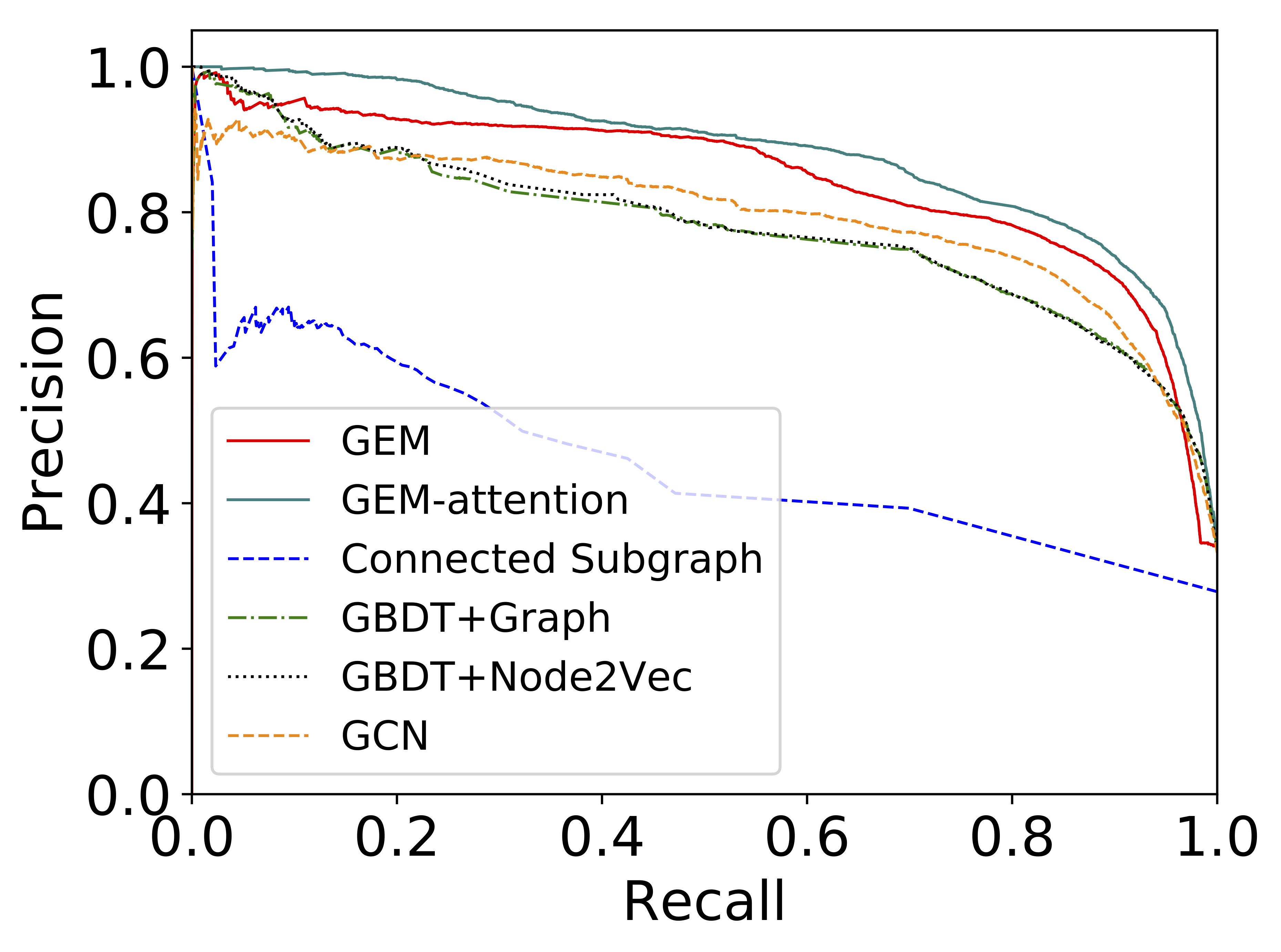
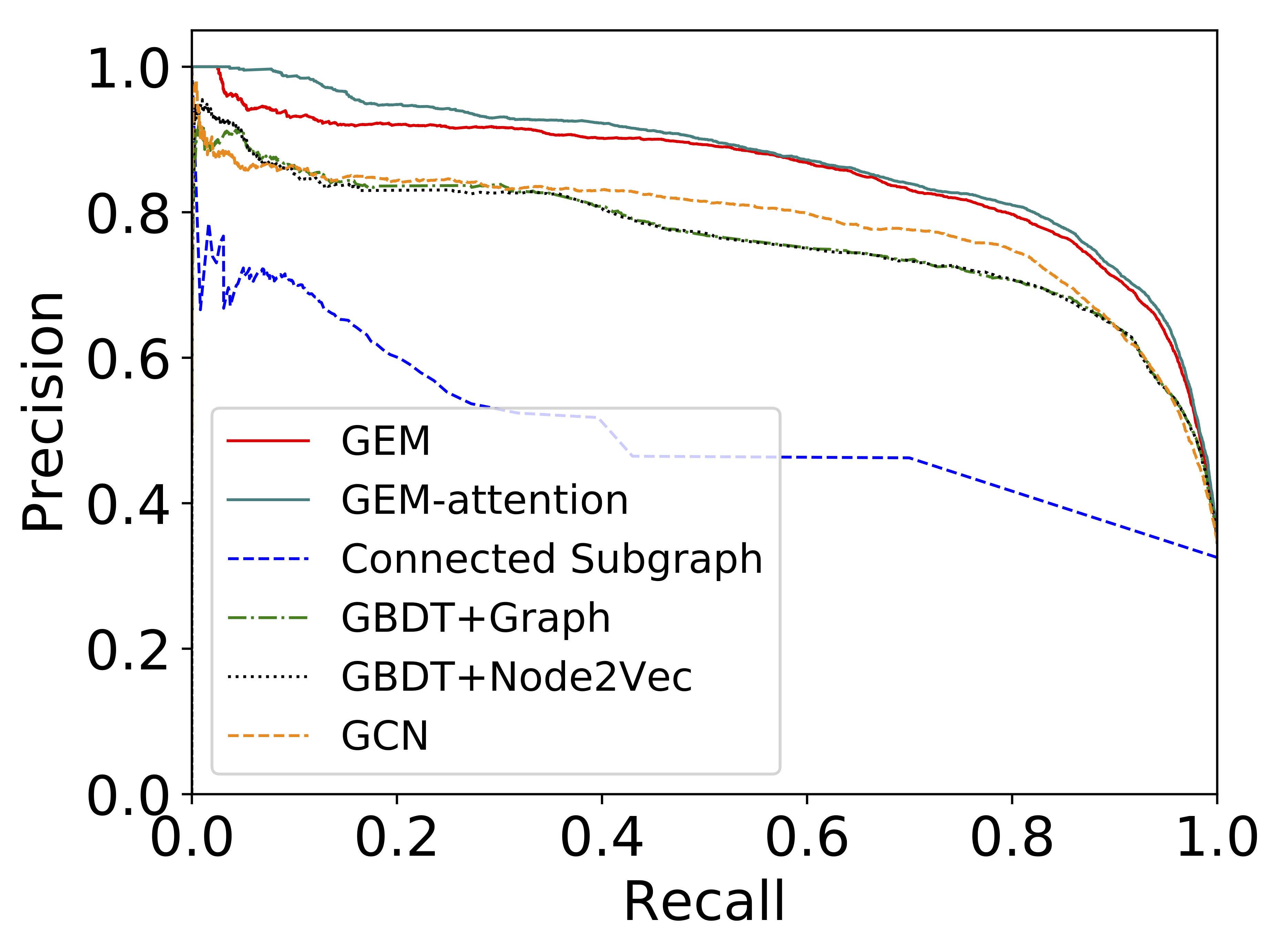
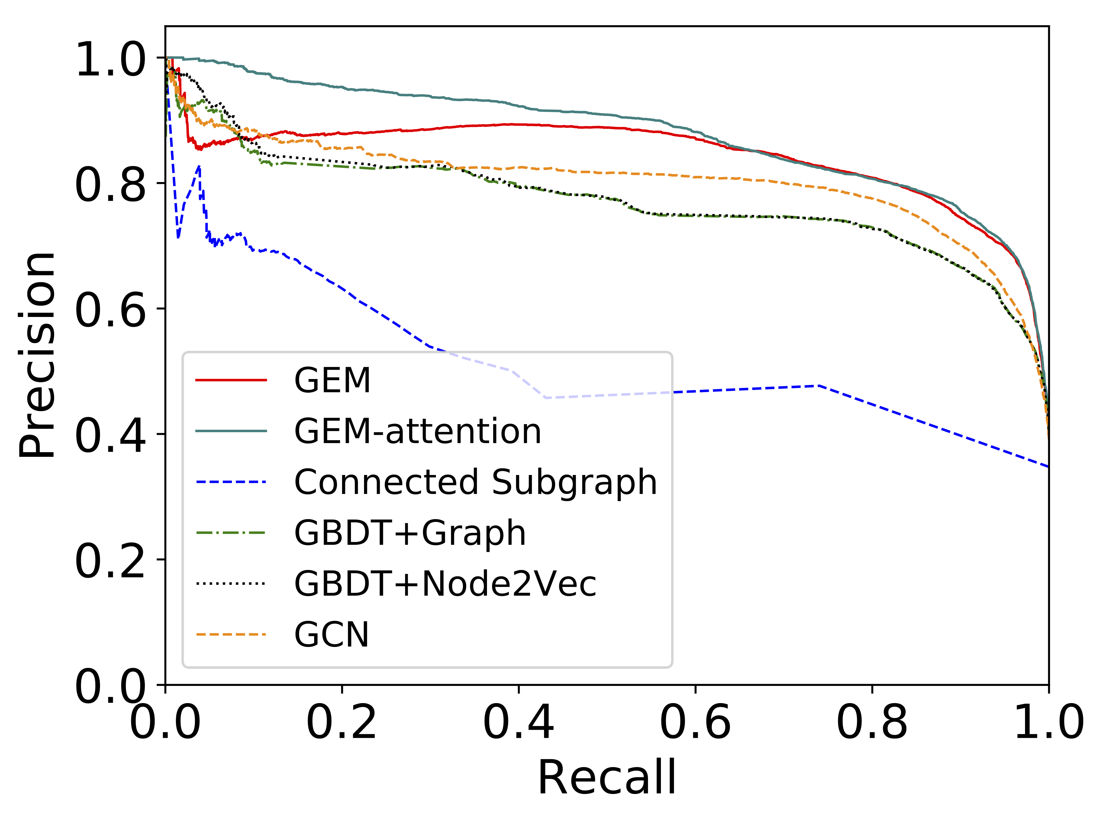
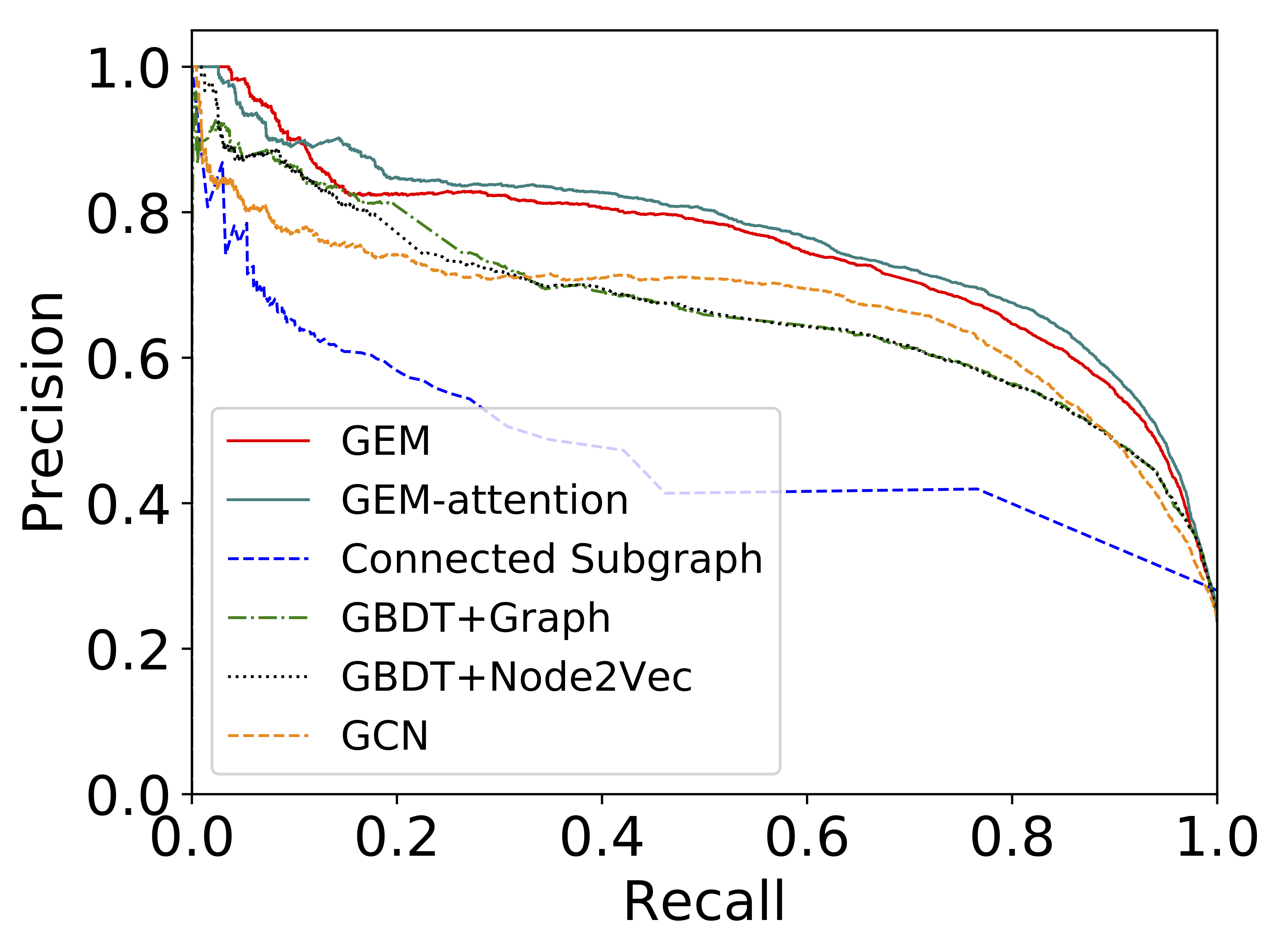
Figure 4. Precision-Recall Curves of GEM, GEM-attention, Connected Subgraph, GBDT+Graph, GBDT+Node2Vec and GCN on test data: week 1 (first), week 2 (second), week 3 (third), week 4 (fourth) .

4.3. Results

4.3.1. Basic Measures

We first report the results of all the methods in terms of standard classification measures, i.e. F-1 scores and AUC in Table 2 and Table 3.

As can be seen, even though the connected subgraph component method is quite intuitive, they are not doing well on this classification problem. The reason is apparrent that large amount of benign accounts interwined with malicious accounts in the device-account graph due to noisy data in practice. There are malicious accouts exist both in large and small connected subgraphs.

The result of GBDT+Graph method is quite similar compared with GBDT+Node2Vec. This might be essentially Node2Vec aims to learn the properties of the graph which is similar to our features extracted in GBDT+Graph.

GCN works better than GBDT+Graph and GBDT+Node2Vec. The reason might be: GCN directly learns node embeddings using the responses of labels and activity features, while the embeddings from Node2Vec or the graph statistics are not optimized for the labels.

Our method GEM consistently outperforms GCN. The reason is two-folds: (1) GEM deals with heterogeneous types of devices compared with GCN that can only deal with homogeneous graphs that GCN can not discern the different types of nodes in graph; (2) GEM uses aggregator operator for each type of nodes instead of normalized operator (Kipf and Welling, 2016) so that it can well model the underlying aggregation patterns as we discussed in section 3.1.

Finally, we find our GEM-attention with attention mechanism that adaptively assigns different attention coefficients to each type of device network performs the best. This is due to the reason that instead of normalizing each type of devices as the same of importance, we should learn their importances from our data because (1) the different types of devices might be noisy in different degrees, for example, IP addresses might be easily confused while UMID could be more unique and accurate; (2) The certain device data could be potentially missing.

4.3.2. Precision-Recall Curves

We report the Precision-Recall curve of all the methods in Figure 4. As we can see, our proposed method GEM significantly outperforms the comparison methods in terms of the area beneath the Precision-Recall curve.

One of the largest connected subgraph consists of a total of 1538 accounts aggregating together in our experimental dataset. The connected subgraph method can precisely identify most of accounts in the largest connected subgraphs as malicious accounts due to the strong signal. This leads to high precision at the very begining of the curve. After that, the precision of the connected subgraph method drops quickly. That is, it is extremely hard for such methods to retain consistent high precision/recall curves when the size of identified connected subgraphs tends to be small.

Our methods work similar or even better at the very begining of the curve compared with the comparison methods. More importantly, our methods can accurately detect much more malicious accounts (high recall) with still relative high precision, which is quite promising.

4.3.3. Model Complexity

In this section, we study the model complexity includes embedding sizes, the depth of hidden convolution layers, and their impact on our task.

Varying Embedding Sizes. We vary embedding sizes from 8, 16, 32, 64 to 128. With larger embedding sizes, we need to add slightly stronger regularizers on our models. With appropriate regularizers, we do not find significant differences in terms of F-1 score.

Varying the Depths of Layers. Indeed, the depth of our hidden convolution layers influences the F-1 scores quite a lot. With deeper hidden layers, our model tends to aggregate transformed information from a neighborhood to a greater extent. We show the F-1 scores with varying depths of hidden layers in Figure 5.

The F-1 score with a depth of 1 hidden layer does not work well because of the heterogeneous graphs we have. Our model needs to “exchange” information among accounts via devices, that requires at least two hops of neighbors to look at.

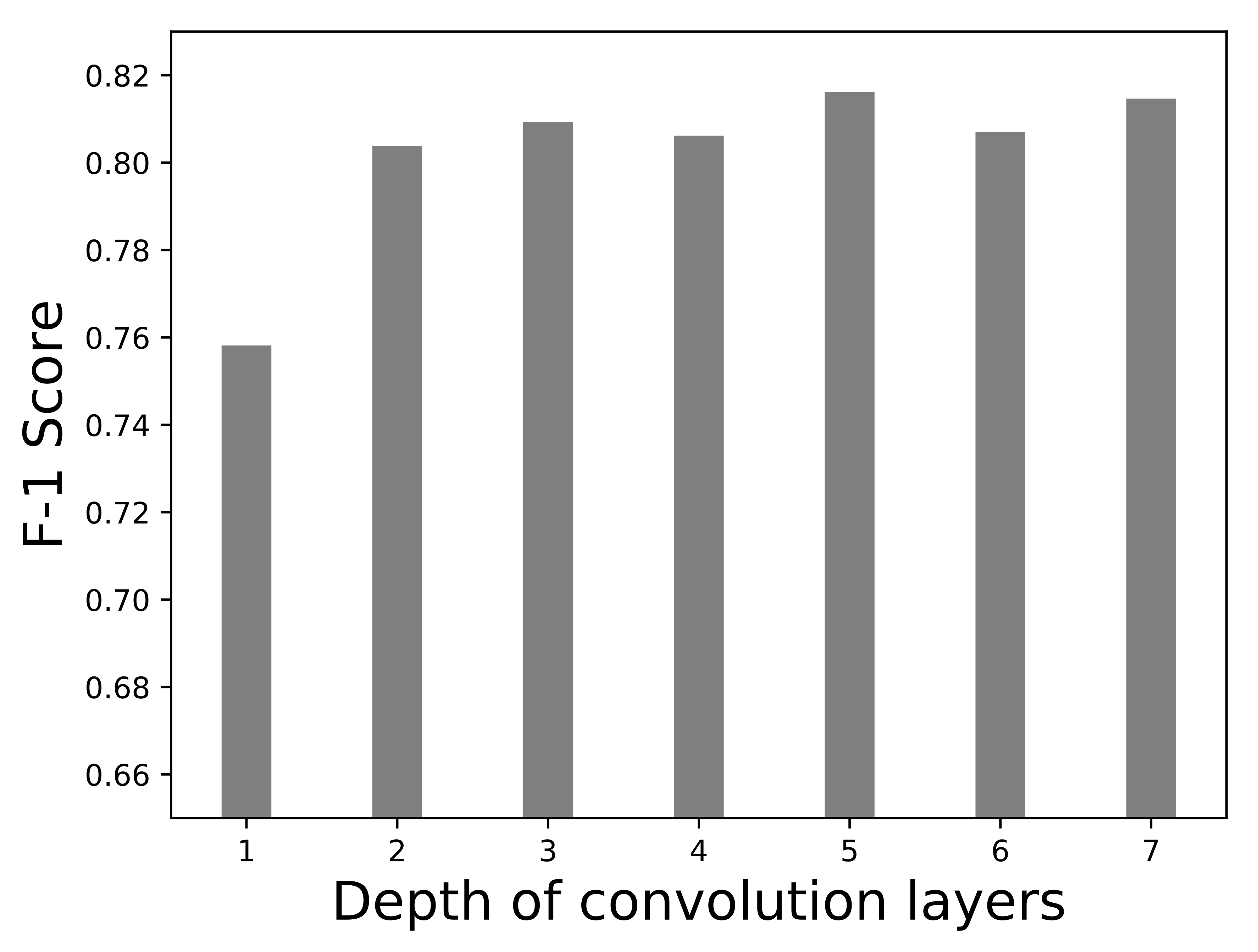
Figure 5. F-1 Score while varying the depths of hidden layers.

4.3.4. Attention Coefficients

In this section, we study the contributions of each type of devices in identifying the malicious accounts by illustrating the estimated attention coefficients using the dataset “week 1”. We show those assigned attention coefficients in table 4. The results show that different types of nodes in a heterogeneous graph could have different impacts on the identification of malicious accounts.

We illustrate one of connected subgraphs with the thicknesses of edges as the corresponding attention coefficients in Figure 3.

Table 4. Assigned attention coefficients estimated using dataset “week 1”.

Devices	Attention coefficients
UMID	0.4412
Phone Number	0.2952
MAC	0.13
APDID	0.1068
IMSI	0.0142
TID	0.0125

4.3.5. Online Results

In practice, everyday we treat top ten thousand scored newly registered accounts identified by our approach as accounts at risk. Under this strategy, the precision evaluated by the security department from Alipay is over 98% after a long time observation. Compared with a former deployed rule-based approach, our GEM can cover 10% more accounts. Thus, we are able to capture more high risk accounts while maintaining very competitive precision.

5. Conclusion

In this paper, we show our experiences on designing novel graph neural networks to detect ten thousands malicious accounts daily at Alipay. In particular, we summarize two fundamental weaknesses of attackers, namely “Device aggregation” and “Activity aggregation”, and naturally present a neural network approach based on heterogeneous account-device graphs. This is the first work that graph neural network approach has ever been applied to fraud detection problems. Our methods achieve promising precision-recall curves compared with competitive methods. Furthermore, we discuss the ideas of re-formulating the intuitive connected subgraph approach to our graph neural network approach. In future, we are interested in building a real-time malicious account detection system based on dynamic graphs instead of the proposed daily detection system.

References

- (1)
- Ahmed et al. (2013) Amr Ahmed, Nino Shervashidze, Shravan Narayanamurthy, Vanja Josifovski, and Alexander J Smola. 2013. Distributed large-scale natural graph factorization. In Proceedings of the 22nd international conference on World Wide Web. ACM, 37–48.
- Bahdanau et al. (2014) Dzmitry Bahdanau, Kyunghyun Cho, and Yoshua Bengio. 2014. Neural machine translation by jointly learning to align and translate. arXiv preprint arXiv:1409.0473 (2014).
- Belkin and Niyogi (2002) Mikhail Belkin and Partha Niyogi. 2002. Laplacian eigenmaps and spectral techniques for embedding and clustering. In Advances in neural information processing systems. 585–591.
- Bruna et al. (2013) Joan Bruna, Wojciech Zaremba, Arthur Szlam, and Yann LeCun. 2013. Spectral networks and locally connected networks on graphs. arXiv preprint arXiv:1312.6203 (2013).
- Cao et al. (2014) Qiang Cao, Xiaowei Yang, Jieqi Yu, and Christopher Palow. 2014. Uncovering large groups of active malicious accounts in online social networks. In Proceedings of the 2014 ACM SIGSAC Conference on Computer and Communications Security. ACM, 477–488.
- Cao et al. (2015) Shaosheng Cao, Wei Lu, and Qiongkai Xu. 2015. Grarep: Learning graph representations with global structural information. In Proceedings of the 24th ACM International on Conference on Information and Knowledge Management. ACM, 891–900.
- Chen and Guestrin (2016) Tianqi Chen and Carlos Guestrin. 2016. Xgboost: A scalable tree boosting system. In Proceedings of the 22nd acm sigkdd international conference on knowledge discovery and data mining. ACM, 785–794.
- Dai et al. (2016) Hanjun Dai, Bo Dai, and Le Song. 2016. Discriminative embeddings of latent variable models for structured data. In International Conference on Machine Learning. 2702–2711.
- Defferrard et al. (2016) Michaël Defferrard, Xavier Bresson, and Pierre Vandergheynst. 2016. Convolutional neural networks on graphs with fast localized spectral filtering. In Advances in Neural Information Processing Systems. 3844–3852.
- Desimone and Duncan (1995) Robert Desimone and John Duncan. 1995. Neural mechanisms of selective visual attention. Annual review of neuroscience 18, 1 (1995), 193–222.
- Gori et al. (2005) Marco Gori, Gabriele Monfardini, and Franco Scarselli. 2005. A new model for learning in graph domains. In Neural Networks, 2005. IJCNN’05. Proceedings. 2005 IEEE International Joint Conference on, Vol. 2. IEEE, 729–734.
- Grover and Leskovec (2016) Aditya Grover and Jure Leskovec. 2016. node2vec: Scalable feature learning for networks. In Proceedings of the 22nd ACM SIGKDD international conference on Knowledge discovery and data mining. ACM, 855–864.
- Hamilton et al. (2017) William L Hamilton, Rex Ying, and Jure Leskovec. 2017. Representation Learning on Graphs: Methods and Applications. arXiv preprint arXiv:1709.05584 (2017).
- He et al. (2016) Kaiming He, Xiangyu Zhang, Shaoqing Ren, and Jian Sun. 2016. Identity mappings in deep residual networks. In European Conference on Computer Vision. Springer, 630–645.
- Huang et al. (2013) Junxian Huang, Yinglian Xie, Fang Yu, Qifa Ke, Martin Abadi, Eliot Gillum, and Z Morley Mao. 2013. Socialwatch: detection of online service abuse via large-scale social graphs. In Proceedings of the 8th ACM SIGSAC symposium on Information, computer and communications security. ACM, 143–148.
- Kipf and Welling (2016) Thomas N Kipf and Max Welling. 2016. Semi-supervised classification with graph convolutional networks. arXiv preprint arXiv:1609.02907 (2016).
- Liu et al. (2018) Ziqi Liu, Chaochao Chen, Longfei Li, Jun Zhou, Xiaolong Li, and Le Song. 2018. GeniePath: Graph Neural Networks with Adaptive Receptive Paths. arXiv preprint arXiv:1802.00910 (2018).
- Perozzi et al. (2014) Bryan Perozzi, Rami Al-Rfou, and Steven Skiena. 2014. Deepwalk: Online learning of social representations. In Proceedings of the 20th ACM SIGKDD international conference on Knowledge discovery and data mining. ACM, 701–710.
- Scarselli et al. (2009) Franco Scarselli, Marco Gori, Ah Chung Tsoi, Markus Hagenbuchner, and Gabriele Monfardini. 2009. The graph neural network model. IEEE Transactions on Neural Networks 20, 1 (2009), 61–80.
- Smola et al. (2007) Alex Smola, Arthur Gretton, Le Song, and Bernhard Schölkopf. 2007. A Hilbert space embedding for distributions. In International Conference on Algorithmic Learning Theory. Springer, 13–31.
- Stringhini et al. (2015) Gianluca Stringhini, Pierre Mourlanne, Gregoire Jacob, Manuel Egele, Christopher Kruegel, and Giovanni Vigna. 2015. Evilcohort: detecting communities of malicious accounts on online services. USENIX.
- Xie et al. (2008) Yinglian Xie, Fang Yu, Kannan Achan, Rina Panigrahy, Geoff Hulten, and Ivan Osipkov. 2008. Spamming botnets: signatures and characteristics. ACM SIGCOMM Computer Communication Review 38, 4 (2008), 171–182.
- Zhao et al. (2009) Yao Zhao, Yinglian Xie, Fang Yu, Qifa Ke, Yuan Yu, Yan Chen, and Eliot Gillum. 2009. BotGraph: Large Scale Spamming Botnet Detection.. In NSDI, Vol. 9. 321–334.