An On-Device Federated Learning Approach for Cooperative Model Update between Edge Devices

Abstract

Most edge AI focuses on prediction tasks on resource-limited edge devices while the training is done at server machines. However, retraining or customizing a model is required at edge devices as the model is becoming outdated due to environmental changes over time. To follow such a concept drift, a neural-network based on-device learning approach is recently proposed, so that edge devices train incoming data at runtime to update their model. In this case, since a training is done at distributed edge devices, the issue is that only a limited amount of training data can be used for each edge device. To address this issue, one approach is a cooperative learning or federated learning, where edge devices exchange their trained results and update their model by using those collected from the other devices. In this paper, as an on-device learning algorithm, we focus on OS-ELM (Online Sequential Extreme Learning Machine) to sequentially train a model based on recent samples and combine it with autoencoder for anomaly detection. We extend it for an on-device federated learning so that edge devices can exchange their trained results and update their model by using those collected from the other edge devices. This cooperative model update is one-shot while it can be repeatedly applied to synchronize their model. Our approach is evaluated with anomaly detection tasks generated from a driving dataset of cars, a human activity dataset, and MNIST dataset. The results demonstrate that the proposed on-device federated learning can produce a merged model by integrating trained results from multiple edge devices as accurately as traditional backpropagation based neural networks and a traditional federated learning approach with lower computation or communication cost.

Keywords On-device learning  $\cdot$ Federated learning  $\cdot$ OS-ELM  $\cdot$ Anomaly detection

1 Introduction

Most edge AI focuses on prediction tasks on resource-limited edge devices assuming that their prediction model has been trained at server machines beforehand. However, retraining or customizing a model is required at edge devices as the model is becoming outdated due to environmental changes over time (i.e., concept drift). Generally, retraining the model later to reflect environmental changes for each edge device is a complicated task, because the server machine needs to collect training data from the edge device, train a new model based on the collected data, and then deliver the new model to the edge device.

To enable the retraining a model at resource-limited edge devices, in this paper we use a neural network based on-device learning approach [1, 2] since it can sequentially train neural networks at resource-limited edge devices and also the neural networks typically have a high flexibility to address various nonlinear problems. Its low-cost hardware implementation is also introduced in [2]. In this case, since a training is done independently at distributed edge devices, the issue is that only a limited amount of training data can be used for each edge device. To address this issue, one approach is a cooperative model update, where edge devices exchange their trained results and update their model using those collected from the other devices. Here we assume that edge devices share an intermediate form of their weight parameters instead of raw data, which is sometimes privacy sensitive.

In this paper, we use the on-device learning approach [1, 2] based on OS-ELM (Online Sequential Extreme Learning Machine) [3] and autoencoder [4]. Autoencoder is a type of neural network architecture which can be applied to unsupervised or semi-supervised anomaly detection, and OS-ELM is used to sequentially train neural networks at resource-limited edge devices. It is then extended for the on-device federated learning so that edge devices can exchange their trained results and update their model using those collected from the other edge devices. In this paper, we employ a concept of Elastic ELM (E²LM) [5], which is a distributed training algorithm for ELM (Extreme Learning Machine) [6], so that intermediate training results are computed by edge devices separately and then a final model is produced by combining these intermediate results. It is applied to the OS-ELM based on-device learning approach to construct the on-device federated learning. Please note that although in this paper the on-device federated learning is applied to anomaly detection tasks since the baseline on-device learning approach [1, 2] is designed for anomaly detection tasks, the proposed approach that employs the concept of E²LM is more general and can be applied to the other machine learning tasks. In the evaluations, we will demonstrate that the proposed on-device federated learning can produce a merged model by integrating trained results from multiple edge devices as accurately as traditional backpropagation based neural networks and a traditional federated learning approach with lower computation or communication cost .

The rest of this paper is organized as follows. Section 2 overviews traditional federated learning technologies. Section 3 introduces baseline technologies behind the proposed on-device federated learning approach. Section 4 proposes a model exchange and update algorithm of the on-device federated learning. Section 5 evaluates the proposed approach using three datasets in terms of accuracy and latency. Section 6 concludes this paper.

2 Related Work

A federated learning framework was proposed by Google in 2016 [8, 9, 10]. Their main idea is to build a global federated model at a server side by collecting locally trained results from distributed client devices. In [10], a secure client-server structure that can avoid information leakage is proposed for federated learning. More specifically, Android phone users train their models locally and then the model parameters are uploaded to the server side in a secure manner.

Preserving of data privacy is an essential property for federated learning systems. In [11], a collaborative deep learning scheme where participants selectively share their models’ key parameters is proposed in order to keep their privacy. In the federated learning system, participants compute gradients independently and then upload their trained results to a parameter server. As another research direction, information leakage at the server side is discussed by considering data privacy and security issues. Actually, a leakage of these gradients may leak important data when the data structure or training algorithm is exposed simultaneously. To address this issue, in [12], an additively homomorphic encryption is used for masking the gradients in order to preserve participants’ privacy and enhance the security at the server side.

Recently, some prior work involved in federated learning focuses on the communication cost or performance in massive or unbalanced data distribution environments. In [13], a compression technique called Deep Gradient Compression is proposed for large-scale distributed training in order to reduce the communication bandwidth.

A performance of centralized model built by a federated learning system depends on statistical nature of data collected from client devices. Typically, data in the client side is not always independent and identically distributed (IID), because clients’ interest and environment are different and sometimes degrade the model performance. In [14], it is shown that accuracy of a federated learning is degraded for highly skewed Non-IID data. This issue is addressed by creating a small subset of data which is globally shared between all the clients. In [15], it is reported that locally trained models may be forgot by a federated learning with Non-IID data, and a penalty term is added to a loss function to prevent the knowledge forgetting.

As a common manner, a server side in federated learning systems has no access to local data in client devices. There is a risk that a client may get out of normal behaviors in the federated model training. In [16], a dimensionality reduction based anomaly detection approach is utilized to detect anomalous model updates from clients in a federated learning system. In [17], malicious clients are identified by clustering their submitted features, and then the final global model is generated by excluding updates from the malicious clients.

Many existing federated learning systems assume backpropagation based sophisticated neural networks but their training is compute-intensive. In our federated learning approach, although we also use neural networks, we employ a recently proposed on-device learning approach for resource-limited edge devices, which will be introduced in the next section. Also, please note that in our approach we assume that intermediate training results are exchanged via a server for simplicity; however, local training and merging from intermediate training results from other edge devices can be completed at each edge device.

3 Preliminaries

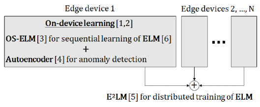
Figure 1: Baseline technologies behind our proposal

This section briefly introduces baseline technologies behind our proposal: 1) ELM (Extreme Learning Machine), 2) E²LM (Elastic Extreme Learning Machine), 3) OS-ELM (Online Sequential Extreme Learning Machine), and 4) autoencoder. Figure 1 illustrates the proposed cooperative model update between $N$ edge devices, each of which performs the on-device learning that combines OS-ELM and autoencoder. Their intermediate training results are merged by using E²LM. Note the original E²LM algorithm is designed for ELM, not OS-ELM; so we modified it so that trained results of OS-ELM are merged, which will be shown in Section 4.

3.1 ELM

ELM [6] is a batch training algorithm for single hidden-layer feedforward networks (SLFNs). As shown in Figure 2, the network consists of input layer, hidden layer, and output layer. The numbers of their nodes are denoted as $n$, $\tilde{N}$, and $m$, respectively. Assuming an $n$-dimensional input chunk $\bm{x}\in\bm{R}^{k\times n}$ of batch size $k$ is given, an $m$-dimensional output chunk $\bm{y}\in\bm{R}^{k\times m}$ is computed as follows.

$$\bm{y}=G(\bm{x}\cdot\bm{\alpha}+\bm{b})\bm{\beta},$$ (1)

where $G$ is an activation function, $\bm{\alpha}\in\bm{R^{n\times\tilde{N}}}$ is an input weight matrix between the input and hidden layers, $\bm{\beta}\in\bm{R^{\tilde{N}\times m}}$ is an output weight matrix between the hidden and output layers, and $\bm{b}\in\bm{R^{\tilde{N}}}$ is a bias vector of the hidden layer.

If an SLFN model can approximate $m$-dimensional target chunk (i.e., teacher data) $\bm{t}\in\bm{R}^{k\times m}$ with zero error ($Loss=0$), the following equation is satisfied.

$$G(\bm{x}\cdot\bm{\alpha}+\bm{b})\bm{\beta}=\bm{t}$$ (2)

Here, the hidden-layer matrix is defined as $\bm{H}\equiv G(\bm{x}\cdot\bm{\alpha}+\bm{b})$. The optimal output weight matrix $\hat{\bm{\beta}}$ is computed as follows.

$$\hat{\bm{\beta}}=\bm{H}^{\dagger}\bm{t},$$ (3)

where $\bm{H}^{\dagger}$ is a pseudo inverse matrix of $\bm{H}$, which can be computed with matrix decomposition algorithms, such as SVD (Singular Value Decomposition) and QRD (QR Decomposition).

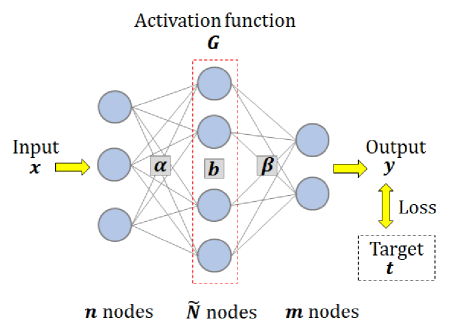
Figure 2: Single hidden-layer feedforward network (SLFN)

In ELM algorithm, the input weight matrix $\bm{\alpha}$ is initialized with random values and not changed thereafter. The optimization is thus performed only for the output weight matrix $\bm{\beta}$, and so it can reduce the computation cost compared with backpropagation based neural networks that optimize both $\bm{\alpha}$ and $\bm{\beta}$. In addition, the training algorithm of ELM is not iterative; it analytically computes the optimal weight matrix $\bm{\beta}$ for a given input chunk in a one-shot manner, as shown in Equation 3. It can always obtain a global optimal solution for $\bm{\beta}$, unlike a typical gradient descent method, which sometimes converges to a local optimal solution.

Please note that ELM is one of batch training algorithms for SLFNs, which means that the model is trained by using all the training data for each update. In other words, we need to retrain the whole data in order to update the model for newly-arrived training samples. This issue is addressed by E²LM and OS-ELM.

3.2 E²LM

E²LM [5] is an extended algorithm of ELM for enabling the distributed training of SLFNs. That is, intermediate training results are computed by multiple machines separately, and then a merged model is produced by combining these intermediate results.

In Equation 3, assuming that rank $\bm{H}=\tilde{N}$ and $\bm{H^{T}}\bm{H}$ is nonsingular, the pseudo inverse matrix $\bm{H}^{\dagger}$ is decomposed as follows.

$$\bm{H^{\dagger}}={(\bm{H^{T}}\bm{H})}^{-1}\bm{H^{T}}$$ (4)

The optimal output weight matrix $\bm{\beta}$ in Equation 3 can be computed as follows.

$$\hat{\bm{\beta}}={(\bm{H^{T}}\bm{H})}^{-1}\bm{H^{T}}\bm{t}$$ (5)

Assuming the intermediate results are defined as $\bm{U}=\bm{H^{T}}\bm{H}$ and $\bm{V}=\bm{H^{T}}\bm{t}$, the above equation is denoted as follows.

$$\hat{\bm{\beta}}=\bm{U}^{-1}\bm{V}$$ (6)

Here, the hidden-layer matrix and target chunk (i.e., teacher data) for newly-arrived training dataset $\Delta\bm{x}$ are denoted as $\Delta\bm{H}$ and $\Delta\bm{t}$, respectively. The intermediate results for $\Delta\bm{x}$ are denoted as $\Delta\bm{U}=\Delta\bm{H^{T}}\Delta\bm{H}$ and $\Delta\bm{V}=\Delta\bm{H^{T}}\Delta\bm{t}$.

Similarly, the hidden-layer matrix and target chunk for updated training dataset $\bm{x}^{\prime}=\bm{x}+\Delta\bm{x}$ are denoted as $\bm{H}^{\prime}$ and $\bm{t}^{\prime}$, respectively. The intermediate results for $\bm{x}^{\prime}$ are denoted as $\bm{U}^{\prime}=\bm{H}^{\prime\bm{T}}\bm{H^{\prime}}$ and $\bm{V^{\prime}}=\bm{H}^{\prime\bm{T}}\bm{t^{\prime}}$. Then, $\bm{U}^{\prime}$ and $\bm{V}^{\prime}$ can be computed as follows.

$$\begin{split}\bm{U}^{\prime}&=\bm{H}^{\prime\bm{T}}\bm{H^{\prime}}={\begin{bmatrix}\bm{H}\\ \Delta\bm{H}\end{bmatrix}}^{T}\begin{bmatrix}\bm{H}\\ \Delta\bm{H}\end{bmatrix}=\bm{H^{T}}\bm{H}+\Delta\bm{H^{T}}\Delta\bm{H}\\ \bm{V}^{\prime}&=\bm{H}^{\prime\bm{T}}\bm{t^{\prime}}={\begin{bmatrix}\bm{H}\\ \Delta\bm{H}\end{bmatrix}}^{T}\begin{bmatrix}\bm{t}\\ \Delta\bm{t}\end{bmatrix}=\bm{H^{T}}\bm{t}+\Delta\bm{H^{T}}\Delta\bm{t}\end{split}$$ (7)

As a result, Equation 7 can be denoted as follows.

$$\begin{split}\bm{U}^{\prime}=\bm{U}+\Delta\bm{U}\\ \bm{V}^{\prime}=\bm{V}+\Delta\bm{V}\end{split}$$ (8)

In summary, E²LM algorithm updates a model in the following steps:

1. Compute $\bm{U}$ and $\bm{V}$ for the whole training dataset $\bm{x}$,

2. Compute $\Delta\bm{U}$ and $\Delta\bm{V}$ for newly-arrived training dataset $\Delta\bm{x}$,

3. Compute $\bm{U}^{\prime}$ and $\bm{V}^{\prime}$ for updated training dataset $\bm{x}^{\prime}$ using Equation 8, and

4. Compute the new output weight matrix $\bm{\beta}$ using Equation 6.

Please note that we can compute a pair of $\bm{U}$ and $\bm{V}$ and a pair of $\Delta\bm{U}$ and $\Delta\bm{V}$ separately. Then, we can produce $\bm{U}^{\prime}$ and $\bm{V}^{\prime}$ by simply adding them using Equation 8. Similar to the addition of $\bm{x}$ and $\Delta\bm{x}$, subtraction and replacement operations for $\bm{x}$ are also supported.

3.3 OS-ELM

OS-ELM [3] is an online sequential version of ELM, which can update the model sequentially using an arbitrary batch size.

Assuming that the $i$-th training chunk $\{\bm{x}_{i}\in\bm{R}^{k_{i}\times n},\bm{t}_{i}\in\bm{R}^{k_{i}\times m}\}$ of batch size $k_{i}$ is given, we need to compute the output weight matrix $\bm{\beta}$ that can minimize the following error.

$$\begin{Vmatrix}\begin{bmatrix}\bm{H}_{0}\\ \vdots\\ \bm{H}_{i}\end{bmatrix}\bm{\beta}_{i}-\begin{bmatrix}\bm{t}_{0}\\ \vdots\\ \bm{t}_{i}\end{bmatrix}\end{Vmatrix},$$ (9)

where $\bm{H}_{i}$ is defined as $\bm{H}_{i}\equiv G(\bm{x}_{i}\cdot\bm{\alpha}+\bm{b})$. Assuming

$$\bm{K_{i}}\equiv{\begin{bmatrix}\bm{H_{0}}\\ \vdots\\ \bm{H_{i}}\end{bmatrix}}^{T}\begin{bmatrix}\bm{H_{0}}\\ \vdots\\ \bm{H_{i}}\end{bmatrix}(i\geq 0),$$ (10)

the optimal output weight matrix is computed as follows.

$$\begin{split}\bm{\beta_{i}}&=\bm{\beta_{i-1}}+\bm{K_{i}^{-1}}\bm{H_{i}^{T}}(\bm{t_{i}}-\bm{H_{i}}\bm{\beta_{i-1}})\\ \bm{K_{i}}&=\bm{K_{i-1}}+\bm{H_{i}^{T}}\bm{H_{i}}\end{split}$$ (11)

Assuming $\bm{P_{i}}\equiv\bm{K_{i}^{-1}}$, we can derive the following equation from Equation 11.

$$\begin{split}\bm{P}_{i}&=\bm{P}_{i-1}-\bm{P}_{i-1}\bm{H}_{i}^{T}(\bm{I}+\bm{H}_{i}\bm{P}_{i-1}\bm{H}_{i}^{T})^{-1}\bm{H}_{i}\bm{P}_{i-1}\\ \bm{\beta}_{i}&=\bm{\beta}_{i-1}+\bm{P}_{i}\bm{H}_{i}^{T}(\bm{t}_{i}-\bm{H}_{i}\bm{\beta}_{i-1})\end{split}$$ (12)

In particular, the initial values $\bm{P}_{0}$ and $\bm{\beta}_{0}$ are precomputed as follows.

$$\begin{split}\bm{P}_{0}&=(\bm{H}_{0}^{T}\bm{H}_{0})^{-1}\\ \bm{\beta}_{0}&=\bm{P}_{0}\bm{H}_{0}^{T}\bm{t}_{0}\end{split}$$ (13)

As shown in Equation 12, the output weight matrix $\bm{\beta}_{i}$ and its intermediate result $\bm{P}_{i}$ are computed from the previous training results $\bm{\beta}_{i-1}$ and $\bm{P}_{i-1}$. Thus, OS-ELM can sequentially update the model with a newly-arrived target chunk in a one-shot manner; thus there is no need to retrain with all the past data unlike ELM.

In this approach, the major bottleneck is the pseudo inverse operation ${(\bm{I}+\bm{H_{i}}\bm{P_{i-1}}\bm{H_{i}^{T}})}^{-1}$. As in [1, 2], the batch size $k$ is fixed at one in this paper so that the pseudo inverse operation of $k\times k$ matrix for the sequential training is replaced with a simple reciprocal operation; thus we can eliminate the SVD or QRD computation.

3.4 Autoencoder

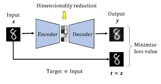
Figure 3: Autoencoder

Autoencoder [4] is a type of neural networks developed for dimensionality reduction, as shown in Figure 3. In this paper, OS-ELM is combined with autoencoder for unsupervised or semi-supervised anomaly detection. In this case, the numbers of input- and output-layer nodes are the same (i.e., $n=m$), while the number of hidden-layer nodes is set to less than that of input-layer nodes (i.e., $\tilde{N}<n$). In autoencoder, an input chunk is converted into a well-characterized dimensionally reduced form at the hidden layer. The process for the dimensionality reduction is denoted as “encoder”, and that for decompressing the reduced form is denoted as “decoder”. In OS-ELM, the encoding result for an input chunk $\bm{x}$ is obtained as $\bm{H}=G(\bm{x}\cdot\bm{\alpha}+\bm{b})$, and the decoding result for the hidden-layer matrix $\bm{H}$ is obtained as $\bm{y}=\bm{H}\cdot\bm{\beta}$.

In the training phase, an input chunk $\bm{x}$ is used as a target chunk $\bm{t}$. That is, the output weight matrix $\bm{\beta}$ is trained so that an input data is reconstructed as correctly as possible by autoencoder. Assuming that the model is trained with a specific input pattern, the difference between the input data and reconstructed data (denoted as loss value) becomes large when the input data is far from the trained pattern. Please note that autoencoder does not require any labeled training data for the training phase; so it is used for unsupervised or semi-supervised anomaly detection. In this case, incoming data with high loss value should be automatically rejected before training for stable anomaly detection.

4 On-Device Federated Learning

As an on-device learning algorithm, in this paper, we employ a combination of OS-ELM and autoencoder for online sequential training and semi-supervised anomaly detection [2]. It is further optimized by setting the batch size $k$ to one, in order to eliminate the pseudo inverse operation of $k\times k$ matrix for the sequential training. A low-cost forgetting mechanism that does not require the pseudo inverse operation is also proposed in [2].

In practice, anomaly patterns should be accurately detected from multiple normal patterns. To improve the accuracy of anomaly detection in such cases, we employ multiple on-device learning instances, each of which is specialized for each normal pattern as proposed in [18]. Also, the number of the on-device learning instances can be dynamically tuned at runtime as proposed in [18].

In this paper, the on-device learning algorithm is extended for the on-device federated learning by applying the E²LM approach to the OS-ELM based sequential training. In this case, edge devices can share their intermediate trained results and update their model using those collected from the other edge devices. In this section, OS-ELM algorithm is analyzed so that the E²LM approach is applied to OS-ELM for enabling the cooperative model update. The proposed on-device federated learning approach is then illustrated in detail.

4.1 Modifications for OS-ELM

Here, we assume that edge devices exchange the intermediate results of their output weight matrix $\bm{\beta}$ (see Equation 6). These intermediate results are obtained by $\bm{U}=\bm{H^{T}}\bm{H}$ and $\bm{V}=\bm{H^{T}}\bm{t}$, based on E²LM algorithm. Please note that the original E²LM approach is designed for ELM, which assumes a batch training, not a sequential training. That is, $\bm{U}$ and $\bm{V}$ are computed by using the whole training dataset. On the other hand, our on-device learning algorithm relies on the OS-ELM based sequential training, in which the weight matrix is sequentially updated every time a new data comes. If the original E²LM approach is directly applied to our on-device learning algorithm, all the past dataset must be preserved in edge devices, which would be infeasible for resource-limited edge devices.

To address this issue, OS-ELM is analyzed as follows. In Equation 11, $\bm{K_{i}}$ is defined as

$$\bm{K_{i}}\equiv{\begin{bmatrix}\bm{H_{0}}\\ \vdots\\ \bm{H_{i}}\end{bmatrix}}^{T}\begin{bmatrix}\bm{H_{0}}\\ \vdots\\ \bm{H_{i}}\end{bmatrix}(i\geq 0),$$ (14)

which indicates that it accumulates all the hidden-layer matrixes that have been computed with up to the $\bm{i}$-th training chunk. In this case, $\bm{U}$ and $\bm{V}$ of E²LM can be computed based on $\bm{K_{i}}$ and its inverse matrix $\bm{P_{i}}$ of OS-ELM as follows.

$$\bm{U_{i}} =\bm{K_{i}}=\bm{P_{i}}^{-1}$$

$$\bm{V_{i}} =\bm{U_{i}}\bm{\beta_{i}},$$ (15)

where $\bm{U_{i}}$ and $\bm{V_{i}}$ are intermediate results for the $\bm{i}$-th training chunk. $\bm{U_{i}}$ and $\bm{V_{i}}$ can be sequentially computed with the previous training results. To support the on-device federated learning, Equation 4.1 is newly inserted to the sequential training algorithm of OS-ELM, which will be introduced in Section 4.2.

4.2 Cooperative Mode Update Algorithm

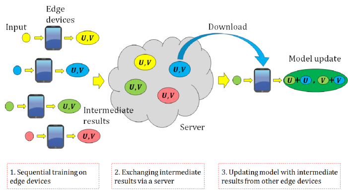
Figure 4: Overview of cooperative model update

Figure 4 illustrates a cooperative model update of the proposed on-device federated learning. It consists of the following three phases:

1. Sequential training on edge devices,

2. Exchanging their intermediate results via a server, and

3. Updating their model with necessary intermediate results from the other edge devices.

First, edge devices independently execute a sequential training by using OS-ELM algorithm. They also compute the intermediate results $\bm{U}$ and $\bm{V}$ by Equation 4.1. Second, they upload their intermediate results to a server. We assume that the input weight matrix $\bm{\alpha}$ and the bias vector $\bm{b}$ are the same in the edge devices. They download necessary intermediate results from the server if needed. They update their model based on their own intermediate results and those downloaded from the server by Equation 8.

Figure 5 shows a flowchart of the proposed cooperative model update between two devices: Device-A and Device-B. Assuming Device-A sends its intermediate results and Device-B receives them for updating its model, their cooperative model update is performed by the following steps.

1. Device-A and Device-B sequentially train their own model by using OS-ELM algorithm. In other words, they compute the output weight matrix $\bm{\beta}$ and its intermediate result $\bm{P}$ by Equation 12.

2. Device-A computes the intermediate results $\bm{U_{A}}$ and $\bm{V_{A}}$ by Equation 4.1 to share them with other edge devices. Device-B also computes $\bm{U_{B}}$ and $\bm{V_{B}}$. They upload these results to a server.

3. Assuming Device-B demands the Device-A’s trained results, it downloads $\bm{U_{A}}$ and $\bm{V_{A}}$ from the server.

4. Device-B integrates their intermediate results by computing $\bm{U_{B}}\leftarrow\bm{U_{A}}+\bm{U_{B}}$ and $\bm{V_{B}}\leftarrow\bm{V_{A}}+\bm{V_{B}}$ by using E²LM algorithm.

5. Device-B updates $\bm{P_{B}}$ and $\bm{\beta_{B}}$ by computing $\bm{P_{B}}\leftarrow\bm{U_{B}}^{-1}$ and $\bm{\beta_{B}}\leftarrow\bm{U_{B}}^{-1}\bm{V_{B}}$.

6. Device-B can execute prediction and/or sequential training of OS-ELM algorithm by using the integrated $\bm{P_{B}}$ and $\bm{\beta_{B}}$.

Edge devices can share their trained results by exchanging their intermediate results $\bm{U}$ and $\bm{V}$ in the proposed on-device federated learning approach, which can mitigate the privacy issues since they do not share raw data for the cooperative model update. Please note that the intermediate results $\bm{U}$ and $\bm{V}$ in Equation 4.1 should be updated only when they are sent to a server or the other edge devices; so there is no need to update them for every input chunk.

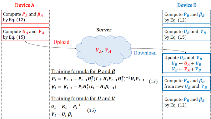
Figure 5: Flowchart of cooperative model update

Regarding the client selection strategy that determines which models of client devices are merged, in this paper we assume a simple case where predefined edge devices share their intermediate trained results for simplicity. Such client selection strategies have been studied recently. For example, a client selection strategy that takes into account computation and communication resource constraints is proposed for heterogeneous edge devices in [19]. A client selection strategy that can improve anomaly detection accuracy by excluding unsatisfying local models is proposed in [20]. Our proposed on-device federated learning can be combined with these client selection strategies in order to improve the accuracy or efficiency, though such a direction is our future work.

5 Evaluations

First, the behavior of the proposed on-device federated learning approach is demonstrated by merging trained results from multiple edge devices in Section 5.2. Then, prediction results using the merged model are compared to those produced by traditional 3-layer BP-NN (backpropagation based neural network) and 5-layer BP-NN in terms of the loss values and ROC-AUC (Receiver Operating Characteristic Curve - Area Under Curve) scores in Section 5.3. Those are also compared to a traditional BP-NN based federated learning approach. In addition, the proposed on-device federated learning is evaluated in terms of the model merging latency in Section 5.4, and it is compared to a conventional sequential training approach in Section 5.5. Table 1 shows specification of the experimental machine.

Table 1: Specification of experimental machine

OS	Ubuntu 17.10
CPU	Intel Core i5 7500 3.4GHz
DRAM	8GB
Storage	SSD 480GB

Table 2: Three datasets

Name	Features	Classes
UAH-DriveSet [21]	225	3
Smartphone HAR [22]	561	6
MNIST [23]	784	10

5.1 Evaluation Environment

5.1.1 Datasets

The evaluations are conducted with three datasets shown in Table 2. Throughout this evaluation, we assume a semi-supervised anomaly detection approach that constructs a model from normal patterns only. In other words, the trained patterns are regarded as normal and the others are anomalous. In this case, a loss value should be low for normal data while it should be high for anomalous data.

UAH-DriveSet [21] contains car driving histories of six drivers simulating three different driving patterns: aggressive, drowsy, and normal. It can be used for the aggressive driving detection. Their car speed was extracted from the GPS data obtained from a smartphone fixed in their cars. The sampling frequency of the car speed was 1Hz. In our experiment, the car speed is quantized with 15 levels (1 level = 10km/h). Assuming a state is assigned to each speed level, we can build a state-transition probability table with 15$\times$15 entries, each of which represents a probability of a state transition from one state to another.

Smartphone HAR dataset [22] contains human activity recordings of 30 volunteers simulating six activities: walking, walking_upstairs, walking_downstairs, sitting, standing, and laying. It can be used for human activity recognition. Their 3-axial linear acceleration and 3-axial angular velocity were captured at a constant rate of 50Hz using waist-mounted smartphone with embedded inertial sensors. The sensor signals were pre-processed. As a result, 561 features consisting of time and frequency domain variables were obtained for each time-window.

MNIST dataset [23] contains handwritten digits from 0 to 9. It is widely used for training and testing in various fields of machine learning. Each digit size is 28$\times$28 pixel in gray scale, resulting in 784 features. In our experiment, all the pixel values are divided by 255 so that they are normalized to [0, 1].

5.1.2 Setup

A vector of 225 features from the car driving dataset, that of 561 features from the human activity dataset, and that of 784 features from MNIST dataset are fed to the neural-network based on-device learning algorithm [2] for anomaly detection. The numbers of input-layer nodes and output-layer nodes are same in all the experiments. The forget factor $\alpha$ is 1 (i.e., no forgetting). The batch size $k$ is fixed to 1. The number of training epochs $E$ is 1. The number of anomaly detection instances is 2 [18]. These instances are denoted as Device-A and Device-B in our experiments. The OS-ELM based anomaly detection with the proposed cooperative model update is implemented with Python 3.6.4 and NumPy 1.14.1. As a comparison with the proposed OS-ELM based anomaly detection, a 3-layer BP-NN based autoencoder and 5-layer BP-NN based deep autoencoder (denoted as BP-NN3 and BP-NN5, respectively) are implemented with TensorFlow v1.12.0 [24]. The hyperparameter settings in OS-ELM, BP-NN3, and BP-NN5 are listed in Table 3. Here, 10-fold cross-validation for ROC-AUC criterion is conducted to tune the hyperparameters with each dataset.

Table 3: Hyperparameter settings

OS-ELM: $\{G_{hidden},p(x),\tilde{N}_{1},L\}$
UAH-DriveSet	$\{$Sigmoid, Uniform, 16, MSE$\}$
Smartphone HAR	$\{$Identity, Uniform, 128, MSE$\}$
MNIST	$\{$Identity, Uniform, 64, MSE$\}$
BP-NN3: $\{G_{hidden},G_{out},\tilde{N}_{1},L,O,k,E\}$
Smartphone HAR	$\{$Relu, Sigmoid, 256, MSE, Adam, 8, 20$\}$
MNIST	$\{$Relu, Sigmoid, 64, MSE, Adam, 32, 5$\}$
BP-NN5: $\{G_{hidden},G_{out},\tilde{N}_{1},\tilde{N}_{2},\tilde{N}_{3},L,O,k,E\}$
Smartphone HAR	$\{$Relu, Sigmoid, 128, 256, 128, MSE, Adam, 8, 20$\}$
MNIST	$\{$Relu, Sigmoid, 64, 32, 64, MSE, Adam, 8, 10$\}$

5.2 Loss Values Before and After Model Update

5.2.1 Setup

Here, we compare loss values before and after the cooperative model update. Below is the experiment scenario using the two instances with the car driving dataset.

1. Device-A trains its model so that the normal driving pattern becomes normal, and the others are anomalous. Device-B trains its model so that the aggressive driving pattern becomes normal, and the others are anomalous.

2. Aggressive and normal driving patterns are fed to Device-A to evaluate the loss values.

3. Device-B uploads its intermediate results to a server, and Device-A downloads them from the server.

4. Device-A updates its model based on its own intermediate results and those from Device-B. It is expected that Device-B’s normal becomes normal at Device-A.

5. The same testing as Step 2 is executed again.

Below is the experiment scenario using the human activity dataset.

1. Device-A trains its model so that the sitting pattern becomes normal, and the others are anomalous. Device-B trains its model so that the laying pattern becomes normal, and the others are anomalous.

2. Walking, walking_upstairs, walking_downstairs, sitting, standing, and laying patterns are fed to Device-B to evaluate the loss values.

3. Device-A uploads its intermediate results to a server, and Device-B downloads them from the server.

4. Device-B updates its model based on its own intermediate results and those from Device-A. It is expected that Device-A’s normal becomes normal at Device-B.

5. The same testing as Step 2 is executed again.

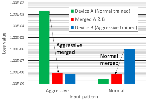
Figure 6: Loss values before and after cooperative model update with car driving dataset

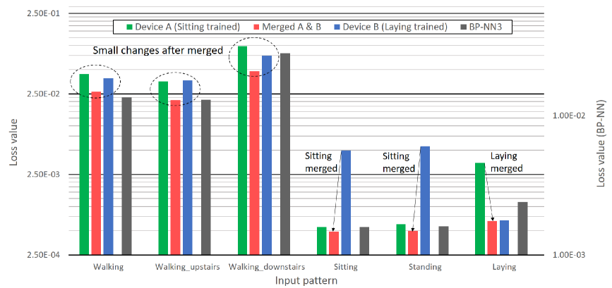
Figure 7: Loss values before and after cooperative model update with human activity dataset

In these scenarios, the loss values at Step 2 are denoted as “before the cooperative model update”. Those at Step 5 are denoted as “after the cooperative model update”. In this setup, after the cooperative model update, “Device-A that has merged Device-B” and “Device-B that has merged Device-A” are identical. A low loss value means that a given input pattern is well reconstructed by autoencoder, which means that the input pattern is normal in the edge device. In the first scenario, Device-A is adapted to the aggressive and normal driving patterns with the car driving dataset. In the second one, Device-B is adapted to the sitting and laying patterns with the human activity dataset.

5.2.2 Results

Figure 6 shows the loss values before and after the cooperative model update with the car driving dataset. X-axis represents the input patterns. Y-axis represents the loss values in a logarithmic scale. Green bars represent loss values of Device-A before the cooperative model update, while red bars represent those after the cooperative model update. Blue bars represent loss values of Device-B. In the case of aggressive pattern, the loss value of Device-A before the cooperative model update (green bar) is high, because Device-A is trained with the normal pattern. The loss value then becomes quite low after integrating the intermediate results of Device-B to Device-A (red bar). This means that the trained result of Device-B is correctly added to Device-A. In the case of normal pattern, the loss value before merging (green bar) is low, but it slightly increases after the trained result of Device-B is merged (red bar). Nevertheless, the loss value is still quite low. We can observe the same tendency for Device-B by comparing the blue and red bars.

Figure 7 shows the loss values before and after the cooperative model update with the human activity dataset. Regarding the loss values, the same tendency with the driving dataset is observed. In the case of sitting pattern, the loss value of Device-B before the cooperative model update (blue bar) is high, because Device-B is trained with the laying pattern. Then, the loss value becomes low after the trained result of Device-A is merged (red bar). In the case of laying pattern, the loss value of Device-A before merging (green bar) is high and significantly decreased after merging of the trained result of Device-B (red bar). On the other hand, in the walking, walking_upstairs, and walking_downstairs patterns, their loss values before and after the cooperative model update are relatively close. These input patterns are detected as anomalous even after the cooperative model update, because they are not normal for both Device-A and Device-B. In the case of standing pattern, the similar tendency as the sitting pattern is observed. The loss value becomes low after the trained result of Device-A is merged to Device-B. This means that there is a similarity between the sitting pattern and standing pattern.

As a counterpart of the proposed OS-ELM based anomaly detection, a 3-layer BP-NN based autoencoder is implemented (denoted as BP-NN3). BP-NN3 is trained with the sitting pattern and laying pattern. In Figure 7, gray bars (Y-axis on the right side) represent loss values of BP-NN3 in a logarithmic scale. Please note that absolute values of its loss values are different from OS-ELM based ones since their training algorithms are different. Nevertheless, the tendency of BP-NN3 (gray bars) is very similar to that of the proposed cooperative model update (red bars). This means that Device-B’s model after the trained result of Device-A is merged can distinguish between normal and anomalous input patterns as accurately as the BP-NN based autoencoder.

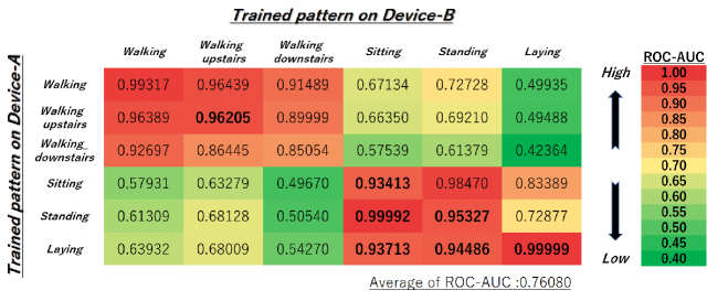
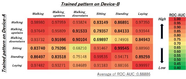
Figure 8: ROC-AUC scores before cooperative model update with human activity dataset

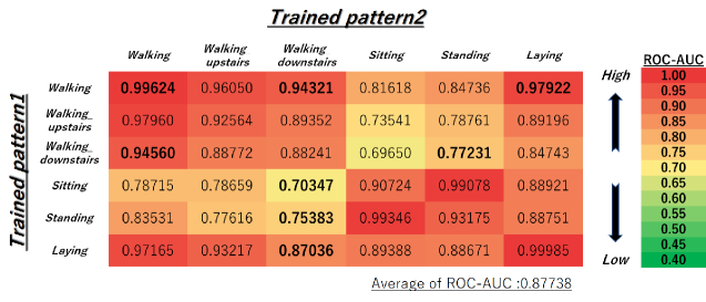
Figure 9: ROC-AUC scores after cooperative model update with human activity dataset

Figure 10: ROC-AUC scores of BP-NN3 with human activity dataset

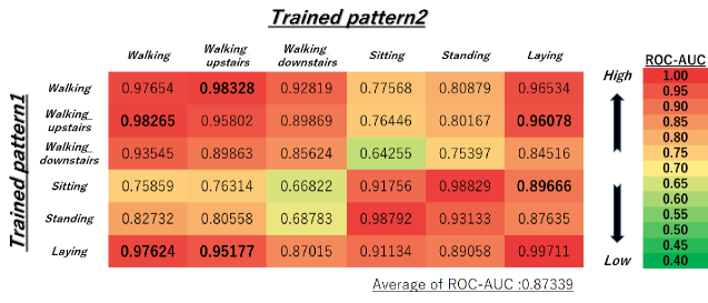
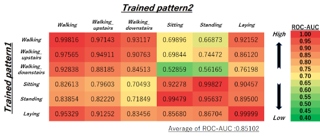
Figure 11: ROC-AUC scores of BP-NN5 with human activity dataset

Figure 12: ROC-AUC scores of traditional FL (BP-NN3-FL) with human activity dataset

5.3 ROC-AUC Scores Before and After Model Update

5.3.1 Setup

Here, ROC-AUC scores before and after the cooperative model update are compared using the human activity dataset and MNIST dataset. The following five steps are performed for every combination of two patterns (denoted as $p_{A}$ and $p_{B}$) in each dataset.

1. Device-A trains its model so that $p_{A}$ becomes normal, and the others are anomalous. Device-B trains its model so that $p_{B}$ becomes normal, and the others are anomalous.

2. ROC-AUC scores are evaluated using all the patterns on Device-A.

3. Device-B uploads its intermediate results to a server, and Device-A downloads them from the server.

4. Device-A updates its model based on its own intermediate results and those from Device-B. It is expected that Device-B’s normal becomes normal at Device-A.

5. The same testing as Step 2 is executed again.

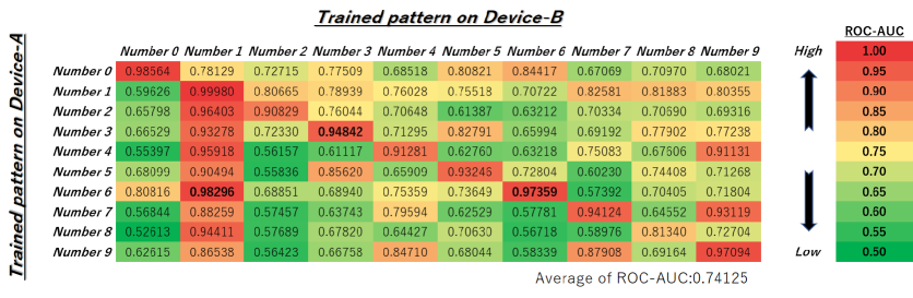
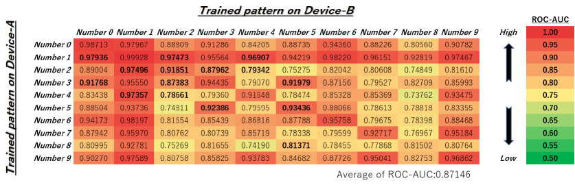
Figure 13: ROC-AUC scores before cooperative model update with MNIST dataset

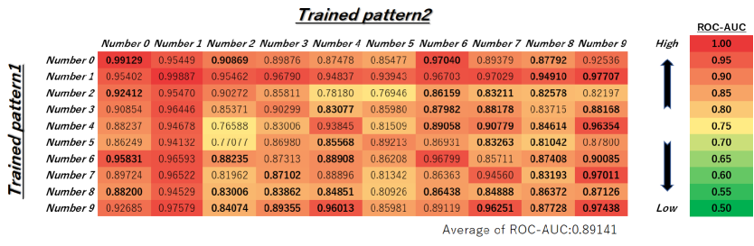
Figure 14: ROC-AUC scores after cooperative model update with MNIST dataset

Figure 15: ROC-AUC scores of BP-NN3 with MNIST dataset

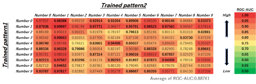
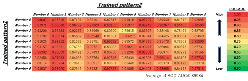
Figure 16: ROC-AUC scores of BP-NN5 with MNIST dataset

Figure 17: ROC-AUC scores of traditional FL (BP-NN3-FL) with MNIST dataset

Trained patterns $p_{A}$ and $p_{B}$ in Step 1 are used as normal test data in Step 2 and Step 5. Whereas, the other untrained patterns are used as anomalous test data. For example, using the human activity dataset, when Device-A is trained with the walking pattern and Device-B is trained with the standing pattern in Step 1, the walking and standing patterns are used as normal data; on the other hand, the other patterns (i.e., walking_upstairs, walking_downstairs, sitting, and laying patterns) are used as anomalous data in Step 2 and Step 5. ROC-AUC scores are evaluated for every combination of patterns with the human activity dataset and MNIST dataset. ROC-AUC scores at Step 2 are denoted as “before the cooperative model update”. Those at Step 5 are denoted as “after the cooperative model update”.

The proposed OS-ELM based federated learning approach is compared to a 3-layer BP-NN based autoencoder (BP-NN3) and a 5-layer BP-NN based deep autoencoder (BP-NN5). BP-NN3 and BP-NN5 train their model so that every combination of two patterns becomes normal. In the case of BP-NN based autoencoders, the two trained patterns are used as normal test data, while the others are used as anomalous test data to evaluate ROC-AUC scores. ROC-AUC scores are calculated for every combination of two patterns in each dataset. In addition, a traditional federated learning approach using BP-NN3 (denoted as BP-NN3-FL) is implemented. In each communication round, two patterns are trained separately based on a single global model. Then, these locally trained models are averaged, and the global model is updated, which will be used for local train of the next round. The number of communication rounds $R$ is set to 50 in all the datasets for stable anomaly detection performance in BP-NN3-FL. Note that $R$ versus accuracy is well analyzed in [10]. Its ROC-AUC scores are calculated as well as BP-NN3 and BP-NN5.

ROC-AUC is widely used as a criterion for evaluating the model performance of anomaly detection independently of particular anomaly score thresholds. ROC-AUC scores range from 0 to 1. A higher ROC-AUC score means that the model can detect both the normal and anomalous patterns more accurately. In this experiment, 80% of samples are used as training data and the others are used as test data in each dataset. The number of anomaly samples in the test dataset is limited to 10% of that of normal samples. The final ROC-AUC scores are averaged over 50 trials for every combination of patterns in each dataset.

5.3.2 Results

Figures 10-12 show ROC-AUC scores with the human activity dataset using heat maps. The highest score among the five models (before and after the cooperative model update, BP-NN3, BP-NN5, and BP-NN3-FL) is shown in bold. Figures 10 and 10 show the results of before and after the proposed cooperative model update. In these graphs, each row represents a trained pattern on Device-A, while each column represents a trained pattern on Device-B. Figures 10-12 show the results of the BP-NN based models, and two trained patterns are corresponding to the row and column. In Figure 10, ROC-AUC scores before the proposed cooperative model update are low especially when trained patterns on Device-A and Device-B have mutually distant features. This is because Device-A is trained with one activity pattern and unseen patterns during the training phase should be detected as anomalous. The ROC-AUC scores are then significantly increased overall after integrating the intermediate results of Device-B to Device-A, as shown in Figure 10. This means that the trained result of Device-B is correctly added to Device-A so that Device-A can extend the coverage of normal patterns in all the combinations of patterns.

In the cases of BP-NN based models shown in Figures 10-12, their tendencies and overall averages of ROC-AUC scores are very similar to those after the proposed cooperative model update. This means that the proposed cooperative model update can produce a merged model by integrating trained results from the other edge devices as accurately as BP-NN3, BP-NN5, and BP-NN3-FL in terms of ROC-AUC criterion. Please note that these BP-NN based models need to be iteratively trained for some epochs in order to obtain their best generalization performance, e.g., they were trained for 20 epochs in BP-NN3 and BP-NN5. In contrast, the proposed OS-ELM based federated learning approach can always compute the optimal output weight matrix only in a single epoch.

Figures 15-17 show ROC-AUC scores with MNIST dataset. We can observe the same tendency with the human activity dataset in the four anomaly detection models. In Figure 15, ROC-AUC scores before the proposed cooperative mode update are low overall except for the diagonal elements, because Device-A is trained with one handwritten digit so that the others should be detected as anomalous on Device-A. Then, the ROC-AUC scores become high even in elements other than the diagonal ones after the trained results of Device-B are merged, as shown in Figure 15. Moreover, a similar tendency as ROC-AUC scores after the proposed cooperative model update is observed in BP-NN3, BP-NN5, and BP-NN3-FL, though average ROC-AUC scores of BP-NN3, BP-NN5, and BP-NN3-FL are slightly higher than those of the proposed cooperative model update, as shown in Figures 15-17. This means that the merged model on Device-A has obtained a comparable anomaly detection performance as the BP-NN based models with MNIST dataset.

5.4 Training, Prediction, and Merging Latencies

5.4.1 Setup

In this section, the proposed on-device federated learning is evaluated in terms of training, prediction, and merging latencies with the human activity dataset. In addition, these latencies are compared with those of the BP-NN3-FL based autoencoder. The batch size $k$ of BP-NN3-FL is set to 1 for a fair comparison with the proposed OS-ELM based federated learning approach. They are compared in terms of the following latencies.

• Training latency is an elapsed time from receiving an input sample until the parameter is trained by using OS-ELM or BP-NN3-FL.

• Prediction latency is an elapsed time from receiving an input sample until its loss value is computed by using OS-ELM or BP-NN3-FL.

• Merging latency of OS-ELM is an elapsed time from receiving intermediate results $\bm{U}$ and $\bm{V}$ until a model update with the intermediate results is finished. That of BP-NN3-FL includes latencies for receiving two locally trained models, averaging them, and optimizing a global model based on the result. It is required for each communication round.

These latencies are measured on the experimental machine shown in Table 1.

Table 4: Training, prediction, and merging latencies [msec]

Number of hidden-layer nodes $\tilde{N}=64$
	Training latency	Prediction latency	Merging latency
OS-ELM	0.471	0.089	5.78
BP-NN3-FL	0.588	0.290	$1.95\times R$
Number of hidden-layer nodes $\tilde{N}=128$
	Training latency	Prediction latency	Merging latency
OS-ELM	0.794	0.106	21.8
BP-NN3-FL	0.980	0.364	$2.42\times R$

5.4.2 Results

Table 4 shows the evaluation results in the cases of $\tilde{N}=64$ and $\tilde{N}=128$. The number of input features is 561. The merging latency of OS-ELM is higher than those of training and prediction latencies, and it depends on the number of hidden-layer nodes because of the inverse operations of $\tilde{N}\times\tilde{N}$ (size of matrix $\bm{U}$ is $\tilde{N}\times\tilde{N}$). Nevertheless, the merging latency is still modest. Please note that the merging latency of BP-NN3-FL is required for each communication round during a training phase, while the merging process of our OS-ELM based federated learning approach is executed only once (i.e., “one-shot”). Thus, the proposed federated learning approach is light-weight in terms of computation and communication costs.

5.5 Convergence of Loss Values

5.5.1 Setup

The proposed cooperative model update can merge trained results of different input patterns at a time. On the other hand, the original OS-ELM can intrinsically adapt to new normal patterns by continuously executing the sequential training of the new patterns. These two approaches (i.e., the proposed merging and the conventional sequential training) are evaluated in terms of convergence of loss values for a new normal pattern using the human activity dataset. The number of hidden-layer nodes $\tilde{N}$ is 128.

In this experiment, Device-A trains its model so that the laying pattern becomes normal, and Device-B trains its model so that the walking pattern becomes normal. In the proposed merging, the trained result of Device-A is integrated to Device-B so that the laying pattern becomes normal in Device-B. In the case of the conventional sequential training, Device-B continuously executes sequential training of the laying pattern, so that the loss value of the laying pattern is gradually decreased. Its decreasing loss value is evaluated at every 50 sequential updates and compared to that of the proposed merging.

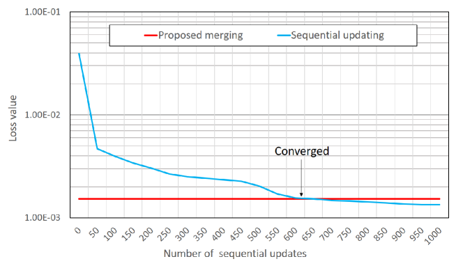
Figure 18: Convergence of loss values of merging and sequential updating

5.5.2 Results

Figure 18 shows the results. X-axis represents the number of sequential updates in the conventional sequential training. Y-axis represents loss values of the laying pattern in a logarithmic scale. Red line represents the loss value of Device-B after the proposed merging; thus, the loss value is low and constant. Blue line represents the loss value of Device-B when sequentially updating its model by the laying pattern; thus, the loss value is decreased as the number of sequential updates increases. Then, the loss value becomes as low as that of the merged one (red line) when the number of sequential updates is approximately 650. For 650 sequential updates, at least $0.794\times 650$ msec is required for the convergence, while the proposed cooperative model update (i.e., merging) requires only 21.8 msec. Thus, the proposed cooperative model update can merge the trained results of the other edge devices rapidly.

6 Conclusions

In this paper, we focused on a neural-network based on-device learning approach so that edge devices can train or correct their model based on incoming data at runtime in order to adapt to a given environment. Since a training is done independently at distributed edge devices, the issue is that only a limited amount of training data can be used for each edge device. To address this issue, in this paper, the on-device learning algorithm was extended for the on-device federated learning by applying the E²LM approach to the OS-ELM based sequential training. In this case, edge devices can share their intermediate trained results and update their model using those collected from the other edge devices. We illustrated an algorithm for the proposed cooperative model update. Evaluation results using the car driving dataset, the human activity dataset, and MNIST dataset demonstrated that the proposed on-device federated learning approach can produce a merged model by integrating trained results from multiple edge devices as accurately as BP-NN3, BP-NN5, and BP-NN3-FL. Please note that the proposed approach is one-shot, which is favorable especially in the federated learning settings since the number of communication rounds significantly affects the communication cost. As a future work, we will explore client selection strategies for our approach in order to further improve the accuracy and efficiency.

References

- [1] Mineto Tsukada, Masaaki Kondo, and Hiroki Matsutani. OS-ELM-FPGA: An FPGA-Based Online Sequential Unsupervised Anomaly Detector. In Proceedings of the International European Conference on Parallel and Distributed Computing (Euro-Par’18) Workshops, pages 518–529, Aug. 2018.
- [2] Mineto Tsukada, Masaaki Kondo, and Hiroki Matsutani. A Neural Network-Based On-device Learning Anomaly Detector for Edge Devices. IEEE Transactions on Computers, 69(7):1027–1044, Jul. 2020.
- [3] N.Y. Liang, G.B. Huang, P. Saratchandran, and N. Sundararajan. A Fast and Accurate Online Sequential Learning Algorithm for Feedforward Networks. IEEE Transactions on Neural Networks, 17(6):1411–1423, Nov. 2006.
- [4] G. Hinton and R. Salakhutdinov. Reducing the Dimensionality of Data with Neural Networks. Science, 313(5786):504–507, Jul. 2006.
- [5] Junchang Xin, Zhiqiong Wang, Luxuan Qu, and Guoren Wang. Elastic Extreme Learning Machine for Big Data Dlassification. Neurocomputing, 149:464–471, Feb. 2015.
- [6] Guang-Bin Huang, Qin-Yu Zhu, and Chee-Kheong Siew. Extreme Learning Machine: A New Learning Scheme of Feedforward Neural Networks. In Proceedings of the International Joint Conference on Neural Networks (IJCNN’04), pages 985–990, Jul. 2004.
- [7] Rei Ito, Mineto Tsukada, and Hiroki Matsutani. An On-Device Federated Learning Approach for Cooperative Model Update between Edge Devices. IEEE Access, 2021. DOI:10.1109/ACCESS.2021.3093382.
- [8] Jakub Konecny, H. Brendan McMahan, Daniel Ramage, and Peter Richtarik. Federated Optimization: Distributed Machine Learning for On-Device Intelligence. arXiv:1610.02527, 2016.
- [9] Jakub Konecny, H. Brendan McMahan, Felix X. Yu, Peter Richtarik, Ananda Theertha Suresh, and Dave Bacon. Federated Learning: Strategies for Improving Communication Efficiency. arXiv:1610.05492, 2016.
- [10] H. Brendan McMahan, Eider Moore, Daniel Ramage, and Blaise Aguera y Arcas. Federated Learning of Deep Networks using Model Averaging. arXiv:1602.05629, 2016.
- [11] Reza Shokri and Vitaly Shmatikov. Privacy-Preserving Deep Learning. In Proceedings of the ACM SIGSAC Conference on Computer and Communications Security (CCS’15), pages 1310–1321, Sep. 2015.
- [12] Le Trieu Phong, Yoshinori Aono, Takuya Hayashi, Lihua Wang, and Shiho Moriai. Privacy-Preserving Deep Learning via Additively Homomorphic Encryption. IEEE Transactions on Information Forensics and Security, 13(5):1333–1345, May 2018.
- [13] Yujun Lin, Song Han, Huizi Mao, Yu Wang, and William J. Dally. Deep Gradient Compression: Reducing the Communication Bandwidth for Distributed Training. arXiv:1712.01887, 2017.
- [14] Yue Zhao, Meng Li, Liangzhen Lai, Naveen Suda, Damon Civin, and Vikas Chandra. Federated Learning with Non-IID Data. arXiv:1806.00582, 2018.
- [15] N. Shoham, T. Avidor, A. Keren, N. Israel, D. Benditkis, L. Mor-Yosef, and I. Zeitak. Overcoming Forgetting in Federated Learning on Non-IID Data. In Proceedings of the International Workshop on Federated Learning for User Privacy and Data Confidentiality in Conjunction with NeurIPS 2019 (FL-NeurIPS’19), Dec. 2019.
- [16] S. Li, Y. Cheng, Y. Liu, W. Wang, and T. Chen. Abnormal Client Behavior Detection in Federated Learning. In Proceedings of the International Workshop on Federated Learning for User Privacy and Data Confidentiality in Conjunction with NeurIPS 2019 (FL-NeurIPS’19), Dec 2019.
- [17] S. Shen, S. Tople, and P. Saxena. AUROR: Defending Against Poisoning Attacks in Collaborative Deep Learning Systems. In Proceedings of the 32nd Annual Conference on Computer Security Applications (ACSAC’16), pages 508–519, Dec. 2016.
- [18] Rei Ito, Mineto Tsukada, Masaaki Kondo, and Hiroki Matsutani. An Adaptive Abnormal Behavior Detection using Online Sequential Learning. In Proceedings of the International Conference on Embedded and Ubiquitous Computing (EUC’19), pages 436–440, Aug. 2019.
- [19] Takayuki Nishio and Ryo Yonetani. Client Selection for Federated Learning with Heterogeneous Resources in Mobile Edge. In Proceedings of the International Conference on Communications (ICC’19), May 2019.
- [20] Yang Qin, Hiroki Matsutani, and Masaaki Kondo. A Selective Model Aggregation Approach in Federated Learning for Online Anomaly Detection. In Proceedings of the International Conference on Cyber Physical and Social Computing (CPSCom’20), pages 684–691, Nov. 2020.
- [21] E. Romera, L. M. Bergasa, and R. Arroyo. Need Data for Driving Behavior Analysis? Presenting the Public UAH-DriveSet. In Proceedings of the International Conference on Intelligent Transportation Systems (ITSC’16), pages 387–392, Nov. 2016.
- [22] Davide Anguita, Alessandro Ghio, Luca Oneto, Xavier Parra, and Jorge L. Reyes-Ortiz. A Public Domain Dataset for Human Activity Recognition Using Smartphones. In Proceedings of the European Symposium on Artificial Neural Networks, Computational Intelligence and Machine Learning (ESANN’13), Apr. 2013.
- [23] Yann LeCun and Corinna Cortes. MNIST handwritten digit database. http://yann.lecun.com/exdb/mnist/, 2010.
- [24] Martín Abadi et al. TensorFlow: Large-Scale Machine Learning on Heterogeneous Systems. https://www.tensorflow.org/.