Non-Anderson critical scaling of the Thouless conductance in 1D

Abstract

We propose and investigate numerically a one-dimensional model which exhibits a non-Anderson disorder-driven transition. Such transitions have recently been attracting a great deal of attention in the context of Weyl semimetals, one-dimensional systems with long-range hopping and high-dimensional semiconductors. Our model hosts quasiparticles with the dispersion $\pm|k|^{\alpha}\operatorname{sign}k$ with $\alpha<1/2$ near two points (nodes) in momentum space and includes short-range-correlated random potential which allows for scattering between the nodes and near each node. In contrast with the previously studied models in dimensions $d<3$, the model considered here exhibits a critical scaling of the Thouless conductance which allows for an accurate determination of the critical properties of the non-Anderson transition, with a precision significantly exceeding the results obtained from the critical scaling of the density of states, usually simulated at such transitions. We find that in the limit of the vanishing parameter $\varepsilon=2\alpha-1$ the correlation-length exponent $\nu=2/(3|\varepsilon|)$ at the transition is inconsistent with the prediction $\nu_{RG}=1/|\varepsilon|$ of the perturbative renormalisation-group analysis. Our results allow for a numerical verification of the convergence of $\varepsilon$-expansions for non-Anderson disorder-driven transitions and, in general, interacting field theories near critical dimensions.

I Introduction

The desire to identify and understand universal critical properties of phase transitions in disordered systems has been motivating, over several decades, advances in numerical and analytical descriptions of disordered and interacting systems, such as new field-theoretical approaches Efetov (1999); Kamenev (2011); Belitz and Kirkpatrick (1994), renormalisation-group methods Dasgupta and Ma (1980); Fisher (1994); Altman et al. (2004); Levitov (1990, 1989); Burin (2006) and scaling theories Cardy (1996). A significant portion of those developments was driven by the studies of the Anderson localisation-delocalisation transitions (see Refs. Mirlin, 2000; Mirlin and Evers, 2000; Efetov, 1999 for a review), commonly believed to be the only possible disorder-driven transitions in non-interacting systems.

The last several years have also seen an upsurge of research activity (see Ref. Syzranov and Radzihovsky, 2018 for a review) on non-Anderson disorder-driven transitions, i.e. disorder-driven transitions in universality classes distinct from those of Anderson localisation. Such transitions (or possibly sharp crossovers ) have been first proposed Fradkin (1986a, b) for Weyl semimetals. They have later been demonstrated Syzranov et al. (2015a); Syzranov and Gurarie (2019); Syzranov and Radzihovsky (2018) to occur in all systems with the power-law quasiparticle dispersion $\propto k^{\alpha}$ in high dimensions Syzranov and Radzihovsky (2018); Syzranov and Gurarie (2019) $d>2|\alpha|$. These systems include, but are not limited to, arrays of trapped ultracold ions which exhibit power-law hopping of excitations Richerme et al. (2014); Islam et al. (2013); Jurcevic et al. (2014, 2015); Rodríguez et al. (2000, 2003); Malyshev et al. (2004); de Moura et al. (2005); Xiong and Zhang (2003); Gärttner et al. (2015), high-dimensional semiconductors, quantum kicked rotors Syzranov and Radzihovsky (2018) and certain disordered supercoductive systems Tikhonov and Feigel’man (2020). Apart from non-Anderson universality classes, such systems display critical scaling of the density of states (which does not exist for Anderson transitions), unconventional behaviour of Lifshitz tails Suslov (1994); Nandkishore et al. (2014); Syzranov et al. (2015b), energy-level statistics and ballistic-transport properties Syzranov and Radzihovsky (2018).

Most studies of the unconventional non-Anderson transitions to date have been focussing on Weyl semimetals, the best known and experimentally available systems predicted to exhibit them. Obtaining the critical exponents at these transitions in Weyl semimetals has been the goal of dozens of analytical and numerical studies (see, e.g., Refs. Shindou and Murakami, 2009; Goswami and Chakravarty, 2011; Ryu and Nomura, 2012; Kobayashi et al., 2014; Syzranov et al., 2015a, b; Louvet et al., 2016; Roy et al., 2018; Syzranov et al., 2016; Pixley et al., 2016; Sbierski et al., 2015; Bera et al., 2016; Liu et al., 2016; Balog et al., 2018).

3D Weyl semimetals do not have any small parameters at the transition point and all analytical methods of their description are, strictly speaking, uncontrolled. In contrast with the Anderson localisation transitions in 3D, certain features of the non-Anderson transitions in Weyl semimetals are described remarkably accurately by means of perturbative one-loop RG calculations controlled by the parameter $\varepsilon=2-d$ with setting $\varepsilon=-1$ at the end of the calculation. For example, the one-loop RG result $z=3/2$ for the dynamical critical exponent $z$ matches the numerical results Kobayashi et al. (2014); Pixley et al. (2016); Sbierski et al. (2015); Bera et al. (2016); Liu et al. (2016) within the error of the numerical simulations (1-2%).

Other results, such as the values of the correlation-length exponent $\nu$, are more controversial (see Ref. Syzranov and Radzihovsky, 2018 for a review): most numerical studies (see, e.g., Refs. Kobayashi et al., 2014; Roy et al., 2018; Pixley et al., 2016, 2015; Sbierski et al., 2015; Bera et al., 2016; Liu et al., 2016; Klier et al., 2019) report errors as large as $10-15\%$, with up to $50\%$ differences in the values of $\nu$ between different studies. The errors in determining the correlation-length exponents at such transitions come from the inaccuracies of the simulations of the critical scaling of the density of states, which have been used to determine the critical properties of the transition in all studies to date, with the exception of Ref. Sbierski et al., 2015 (where a finite-size analysis of the conductance has been carried out). Because the density of states vanishes or nearly vanishes on one side of a non-Anderson transition, accurate determination of the transition point is challenging, which may lead to substantial errors in determining the correlation-length exponent. Furthermore, the transition point may be additionally obscured by rare-region effects, whose role is also being debated in the literature Note (1).

These controversies, together with the need for better understanding of non-Anderson criticality, has motivated us to propose and study in this paper a model exhibiting non-Anderson disorder-driven transitions which, on the one hand, is controlled by a small tunable parameter $|\varepsilon|\ll 1$ and, on the other hand, exhibits the critical scaling of a non-vanishing observable allowing for an accurate determination of the critical properties.

We study a one-dimensional disordered chain where the quasiparticle dispersion hosts two nodes, i.e. points with the chiral dispersion $\pm|k|^{\alpha}\operatorname{sign}k$, where the momentum $k$ is measured from each node and $\alpha<1/2$. While transitions in one-dimensional models with power-law dispersions have been studied numerically previously Rodríguez et al. (2000, 2003); Malyshev et al. (2004); de Moura et al. (2005); Xiong and Zhang (2003); Gärttner et al. (2015), the model considered here combines several ingredients which allow us to determine the critical properties of the transition rather precisely.

On the one hand, the energies of the nodes are robust against disorder (similarly to that in Ref. Gärttner et al., 2015 and in contrast with Refs. Rodríguez et al., 2000, 2003; Malyshev et al., 2004; de Moura et al., 2005; Xiong and Zhang, 2003), which is essential for the accurate identification of the transition point, as the non-Anderson disorder-driven transition takes place for states at only one energy. On the other hand, the system exhibits a critical scaling of the Thouless conductance, a quantity which, unlike the density of states, remains finite at the transition.

The finite-size scaling analysis of the Thouless conductance allows us to obtain the correlation-length exponent as a function of the parameter $\varepsilon=2\alpha-1$ and compare the result with the prediction of the analytical perturbative-RG descriptions controlled by the small parameter $\varepsilon$. We find that, contrary to the common expectation, the numerical result for the correlation-length exponent is inconsistent with the predictions of the perturbative RG approaches.

As non-Anderson disorder-driven transitions may be described by deterministic interacting field theories in the replica, supersymmetric or Keldysh representations, the approach we develop here may be used more broadly to verify the convergence of the $\varepsilon$-expansions in interacting field theories.

II Summary of the results

In this work, we focus on the numerical analysis of the correlation length-exponent $\nu(\varepsilon)$ as a function of the parameter $\varepsilon=2\alpha-1$, where $\alpha$ characterises the dispersion $\pm k^{\alpha}\operatorname{sign}k$ near several points (nodes) in momentum space (see Sec. III for a full description of the model and Eq. (3) for the dispersion for all momenta).

We use the critical scaling of a quantity similar to the Thouless conductance $g$, introduced in Sec. IV, for an accurate determination of the correlation-length exponent for the parameter $|\varepsilon|$ in the interval $|\varepsilon|=0.1\ldots 0.5$. Studying the critical properties of the transition for $|\varepsilon|\ll 1$ allows us not only to compare the numerical results with the analytical perturbative RG predictions, justified in the limit of small $\varepsilon$, but also to neglect possible non-perturbative rare-region effects Note (1), exponentially suppressed Syzranov et al. (2015b); Syzranov and Radzihovsky (2018) by the parameter $1/|\varepsilon|$.

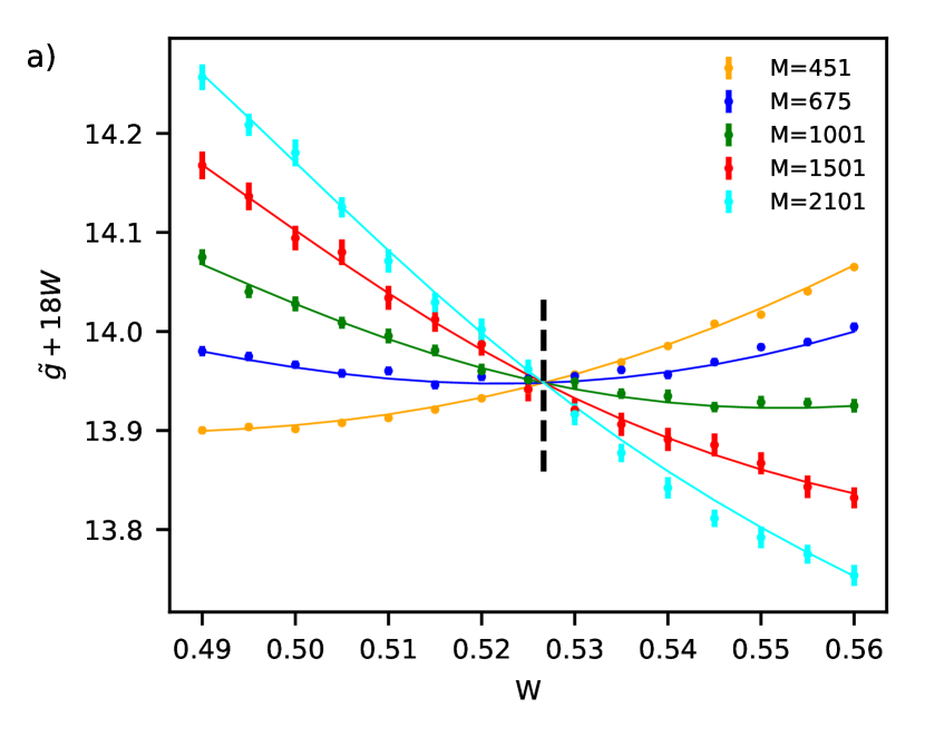
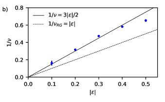
Figure 1: Results for the critical properties of the non-Anderson disorder-driven transition. (a) Median $\tilde{g}$ of the Thouless conductance distribution for various system sizes $L=2M$ and disorder amplitudes $W$. The solid lines show the fourth-order polynomial fit of the scaling function $\tilde{g}\left[u\left(W-W_{c}\right)L^{1/\nu}\right]$ with $u(w)=w+bw^{2}$ (see Appendix A). The vertical line shows the critical amplitude $W=W_{c}$ obtained from the fit. The linear function $18W$ is added to the conductance $\tilde{g}$ on the vertical axis for better visibility of the crossing. (b) The inverse correlation-length exponent $1/\nu$, obtained from the scaling analysis for various $\varepsilon$, as a function of $\varepsilon$. The solid line shows the dependence $1/\nu=3|\varepsilon|/2$, which describes accurately the numerical data in the limit of small $\varepsilon$, in contrast with the prediction $1/\nu_{RG}=|\varepsilon|$ of the analytical RG approach showed by the dashed line.

Our results for the critical properties are summarised in Fig 1. Panel (a) shows the finite-size scaling of the median $\tilde{g}$ of the conductance distribution as a function of the system size and disorder strength for representative $\alpha=0.4$ ($|\varepsilon|=0.2$). For strong disorder, $\tilde{g}$ decreases with system size $L$, whereas the opposite trend is observed for weak disorder. These regimes are separated by a critical disorder amplitude $W_{c}$, a unique crossing point for data traces pertaining to different system sizes. Around $W_{c}$, we fit the data with a polynomial scaling function (solid lines) to find the correlation-length exponent $\nu$. Based on the data for five different values of $\varepsilon$, we find the asymptotic dependence (Fig. 1b)

$$\frac{1}{\nu}=\frac{3}{2}|\varepsilon|.$$ (1)

Surprisingly, this result is in contradiction with the prediction of the perturbative one-loop RG analysis,

$$\frac{1}{\nu_{RG}}=|\varepsilon|,$$ (2)

believed to be exact in the limit of $\varepsilon\rightarrow 0$. We present the details of the analytical RG analysis for the model under consideration in Appendix B.

As further checks of this unexpected result, we (i) confirm the consistency of our value of $\nu(|\varepsilon|=0.2)=3.163\pm 0.041$ with the scaling analysis of the density of states (see Sec. V and Fig. 4), and (ii) find an unusual scaling of the critical dimensionless disorder strength $\gamma_{c}\propto|\varepsilon|^{2/3}$ (Fig. 5) which also contradicts the predictions of the analytical RG approach but is consistent with earlier results for a similar one-dimensional model.de Moura et al. (2005)

III Model and Observable

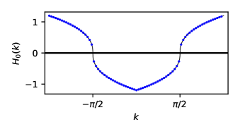
Figure 2: The dispersion $H_{0}(k)$ in a disorder-free system as a function of $k$ for $\alpha=0.4$. The solid line depicts the continuum dispersion while the blue points indicate the placement of discrete momenta ($M=41$) in the finite-size version of the model.

We consider a model described by the Hamiltonian

$$H_{0}(k)=\begin{cases}\left|k-\pi/2\right|^{\alpha}\,\operatorname{sign}(k-\pi/2),&0<k<\pi,\\ \left|k+\pi/2\right|^{\alpha}\,\operatorname{sign}(k+\pi/2),&-\pi<k<0,\\ \infty,&\mathrm{otherwise}.\end{cases}$$ (3)

The dispersion is depicted in Fig. 2. Near the momenta $k=\pm\pi/2$, hereinafter referred to as nodes, the dispersion has the power-law form and lacks reflection symmetry.

The singular dispersion $\propto|k\pm\pi/2|^{\alpha}\operatorname{sign}(k\pm\pi/2)$ near the nodes corresponds to the power-law hopping $\propto 1/|x|^{1+\alpha}\operatorname{sign}x$ in coordinate space at large distances $x$. Disorder-driven transitions in similar models with power-law hopping, corresponding to the dispersion $\propto k^{\alpha}$ which is even with respect to the momentum inversion $k\rightarrow-k$), have been studied numerically in Refs. Rodríguez et al., 2000, 2003; Malyshev et al., 2004; de Moura et al., 2005; Xiong and Zhang, 2003. Because the dispersion considered here is odd with respect to inverting the momentum measured from the node and the momentum states with energies above and below the nodes have equal weights, the energies of the nodes are not renormalised if the system is exposed to quenched short-range-correlated disorder with zero average. Because only the states at the node energies undergo the non-Anderson disorder-driven transitions, the absence of the renormalisation of the energies of the nodes helps us identify such states more accurately.

A model with the dispersion $\propto k^{\alpha}\operatorname{sign}k$, the single-node version of the dispersion (3), has been studied in Ref. Gärttner et al., 2015. In that model, the quasiparticles can move only in one direction and cannot be backscattered. By contrast, the dispersion considered here allows for the scattering between the two nodes in the presence of the random potential, which leads to the critical scaling of a quantity similar to the Thouless conductance, Edwards and Thouless (1972); Thouless (1974) which we describe below. The Thouless conductance does not vanish at the critical point, unlike the density of states, and thus allows for a significantly more precise determination of the critical properties of the transition.

We discretise the dispersion (3) on a lattice in momentum space and represent the dispersion in the form $H_{0}=\sum_{k}\left|k\right\rangle H_{0}(k)\left\langle k\right|$ where the sum runs over $k_{m}=\frac{2\pi m}{L}$ with $m=-M,...,M-1$. Here, $M$ is an odd integer and $L=2M$. These $k$-points fall symmetrically around the nodes while avoiding the momenta $\pm\pi/2$ of the nodes. The density of states in the absence of disorder is given by $\rho_{\text{clean}}(E)=2\left|E\right|^{1/\alpha-1}/(2\pi\alpha)$, where the energy $E$ is measured from the energies of the nodes.

We generate disorder on a real-space grid of $4M$ sites with spacing $1/2$. On each lattice site $i$, the disorder potential $U_{i}$ is drawn from a box distribution $U_{i}\in\left[-\sqrt{3}W,+\sqrt{3}W\right]$ leading to the disorder averaged correlator $\left\langle U_{i}U_{j}\right\rangle_{\text{dis}}=\delta_{i,j}W^{2}$. In addition, we subtract the mean for each disorder realisation to ensure $\sum_{i}U_{i}=0$. We then Fourier-transform the generated random potential, $U=\sum_{k\neq k^{\prime}}\left|k^{\prime}\right\rangle U(k^{\prime}-k)\left\langle k\right|$. Because the potential is real, $U(k)=U^{\star}(-k)$. We emphasise that, since the dispersion (3) is not periodic in momentum space, there is no Umklapp scattering in our model.

The eigenstates of the Hamiltonian $H=H_{0}+U$ are found by exact diagonalisation. We note that the Hamiltonian matrix in coordinate space is not sparse due to the long-range character of the hopping.

Scaling observable. In what immediately follows, we describe a quantity similar to the Thouless conductance, which we use in order to identify the non-Anderson disorder-driven transition. The Thouless conductance Edwards and Thouless (1972); Thouless (1974); Braun et al. (1997) is usually defined (up to a coefficient of $1/\delta$, with $\delta$ being the mean level spacing) as a response of the energy $E_{n}$ of an eigenstate $\left|n\right\rangle$ to an adiabatic twist of the phase $\phi$ in the boundary conditions Thouless (1974). Such a twist for the system considered here corresponds to the replacement $k\rightarrow k+\frac{2\pi}{L}\phi$ in the dispersion (3).

In order to study the criticality, we analyse the quantity

$$g=\left|{\partial_{\phi}^{2}E_{n_{0}}|_{\phi=0}}/{E_{n_{0}}}\right|,$$ (4)

where $E_{n_{0}}$ is the energy, measured from the node energy, of the eigenstate $n_{0}$ with the smallest absolute value $|E_{n_{0}}|$ at $\phi=0$. The Thouless conductance Edwards and Thouless (1972); Thouless (1974); Braun et al. (1997) in systems with a constant density of states in a certain energy interval matches Eq. (4) with the replacement $E_{n_{0}}\rightarrow\delta$, where $\delta$ is the mean level spacing in the respective interval. While the density of states in the system considered here vanishes at the nodes, the quantity $E_{n_{0}}$ in Eq. (4) plays a role similar to that of the mean level spacing $\delta$ in the conventional definition of the Thouless conductance. For simplicity, we refer to the quantity (4) as the Thouless conductance in the rest of the paper.

According to the second-order perturbation theory, a phase twist of $\phi$ at the boundary of the system is equivalent to adding the perturbation $H_{\phi}(k)\simeq\left(\frac{2\pi}{L}\phi\right)h_{\phi}^{(1)}(k)+\frac{1}{2}\left(\frac{2\pi}{L}\phi\right)^{2}h_{\phi}^{(2)}(k)$ to the Hamiltonian $H$, where

$$h_{\phi}^{(1)}(k) =\mp\alpha|k\pm k_{0}|^{\alpha-1},$$ (5)

$$h_{\phi}^{(2)}(k) =\mp\alpha\left(\alpha-1\right)\mathrm{sgn}(k\pm k_{0})|k\pm k_{0}|^{\alpha-2},$$ (6)

with the upper and lower sign corresponding, respectively, to $0<k<\pi$ and $-\pi<k<0$. The terms of higher orders in $\phi$ do not affect the Thouless conductance defined by Eq. (4). We emphasise that the discretisation of momenta, which we use in this paper, allows us to avoid non-analyticities of $H_{0}(k)$ at the nodal points at $k=\pm\pi/2$. Utilising Eqs. (5)-(6), we obtain

$$\partial_{\phi}^{2}E_{n_{0}}|_{\phi=0}=\left(\frac{2\pi}{L}\right)^{2}\left[\left\langle n_{0}|h_{\phi}^{(2)}\left(k\right)|n_{0}\right\rangle\right.$$

$$\left.+2\sum_{m\neq n_{0}}\frac{\left|\left\langle m|h_{\phi}^{(1)}\left(k\right)|n_{0}\right\rangle\right|^{2}}{E_{n_{0}}-E_{m}}\right].$$ (7)

In the numerical analysis described below, we use Eq. (7) in order to determine numerically the Thouless conductance defined by Eq. (4).

IV Scaling of Thouless conductance

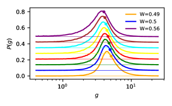
Figure 3: Normalized probability distribution of the Thouless conductance obtained for $\sim 10^{5}$ disorder realizations in the case $\alpha=0.4$, $M=451$ and $W=0.49,0.50,...,0.56$ (bottom to top). The dot indicates the position of the median conductance $\tilde{g}$. Each curve is offset vertically for better visibility, with the thin horizontal line corresponding to vanishing probability density.

Near a continous phase transition, the universal critical exponent $\nu$ describes the divergence of the correlation length Cardy (1996) $\xi\propto|w|^{-\nu}$ as a function of the tuning parameter that vanishes at the transition point. In this paper, we use the deviation $w=W-W_{c}$ of the disorder amplitude $W$ from the critical value $W_{c}$ as the tuning parameter.

The exponent $\nu$ may be determined from the behaviour of a dimensionless observable $\tilde{g}$ that depends on the system size $L$ only via the dimensionless ratio $L/\xi$, or, equivalently $\tilde{g}(W,L)=\tilde{g}(wL^{1/\nu})$. In particular, the critical amplitude $W_{c}$ may be found as the amplitude at which $\tilde{g}(W,L)$ is independent of the system size $L$. The exponent $\nu$ may then be obtained from a polynomial fitting procedure. Slevin and Ohtsuki (1999, 2009, 2014)

The outstanding challenge in the context of the non-Anderson transition is to find an appropriate scaling variable. The density of states at zero energy, commonly used for the studies of such transitions Syzranov and Radzihovsky (2018), or its dimensionless generalisations, are not suitable for finite-size scaling analysis due to the vanishing of the density of states at the transition point (possibly up small contributions from rare-region effects Suslov (1994); Nandkishore et al. (2014); Syzranov et al. (2015b); Buchhold et al. (2018a); Note (1)). Here, we demonstrate numerically that the Thouless conductance defined by Eq. (4) is a suitable scaling variable.

In Fig. 3 we show the probability density of the Thouless conductance for $\alpha=0.4$ and $M=451$, obtained for $\sim 10^{5}$ disorder realizations. The distribution function $P(g)$ is approximately log-Gaussian. The scaling hypothesis discussed above applies also to the distribution function $P(g)$. As it is not practical to work with the full distribution, in what follows we restrict ourselves to the scaling analysis of only the median $\tilde{g}$. We note, however, that choosing the typical conductance $\mathrm{exp}(\overline{\mathrm{ln}\,g})$ yields rather similar results. The standard error of the median conductance is calculated using the asymptotic variance formula $\sigma_{\tilde{g}}^{2}=1/[4P(\tilde{g})^{2}n]$, where $n$ is the total number of disorder realisations for a particular data point $(W,L)$ and the probability density is approximated by a smooth interpolation of the observed histogram.

In Fig. 1a , we plot $\tilde{g}(W,L)$ for $\alpha=0.4$ (corresponding to $|\epsilon|=0.2$) over a range of disorder strengths $W$ and for various system sizes $L$. We observe that data traces for different $L$ cross at one point, demonstrating the critical scaling behaviour. To check further the validity of the scaling hypothesis and extract the correlation-length exponent $\nu$, we use the polynomial fitting procedureSlevin and Ohtsuki (1999, 2009, 2014) detailed in Appendix A. This procedure relies on expanding the scaling function $\tilde{g}[u(w)L^{1/\nu}]$ as a low-order polynomial and allows for quadratic and higher-order corrections in the dependence of the relevant scaling variable $u(w)=w+{\cal O}(w)$ on $w$. The parameters $\nu$ and $W_{c}$ and the polynomial coefficients are obtained from a least-squares fit (solid lines).

For $\alpha=0.4$ ($|\varepsilon|=0.2$), we find $\nu=3.163\pm 0.041$. We use the same method to determine the critical exponent $\nu$ for all values of $\alpha$ (see Appendix A). The results for $\nu$ and $W_{c}$ as a function of $\varepsilon=2\alpha-1$ are shown, respectively, in Figs. 1b and 5.

V Scaling of the density of states

Most studies to date have relied on the scaling form Kobayashi et al. (2014) of the density of states for the numerical determination of the critical exponents. In what immediately follows, we demonstrate that the scaling of the density of states in the model considered here is consistent with the results obtained from the finite-size scaling analysis of the Thouless conductance.

As discussed in Sec. IV, simulating numerically the density of states does not allow for an accurate determination of the critical disorder amplitude $W_{c}$, which is why we use the result $W_{c}=0.5267$ obtained from the finite-size scaling of the Thouless conductance to fit the scaling of the density of states for a system with $\alpha=0.4$. The disorder-averaged density of states $\rho(E\approx 0)$ for the system size $M=8001$ and various disorder strengths around $W_{c}$ is shown in Fig. 4a.

We obtain that the density of states $\rho(E\approx 0,W)$ is strongly suppressed for $W\leq W_{c}$ and grows rapidly at larger $W$. Our results are consistent, to a good accuracy, with the scaling form Kobayashi et al. (2014)

$$\rho(E=0,W>W_{c})\propto(W-W_{c})^{(1-z)\nu},$$ (8)

where $z$ is the dynamical critical exponent, given by $z=1/2+{\cal O}(\varepsilon)$ according to the perturbative RG calculations. Numerically, the value of the dynamical exponent may be obtained from the scaling of the integrated density of states (i.e. the number of states with energies between $0$ and $E$) $N(E)=\int_{0}^{E}d\epsilon\,\rho(\epsilon)\propto E^{1/z}$ at $W=W_{c}$. Our data for $W=0.53$ close to $W_{c}$ is consistent with $z=1/2$ (dashed line) within a few-percent error.

In Fig. 4c, we show the numerical data for $\rho(E=0,W>W_{c})$ vs. $W-W_{c}$ in a log-log plot (dots). The dependence is consistent with Eq. (8) with the correlation-length exponent $\nu=3.163$ obtained from the finite-size scaling above (solid line). On the contrary, the prediction $\nu_{RG}=1/|\varepsilon|$ of the one-loop RG (dashed line) is clearly inconsistent with the numerical data.

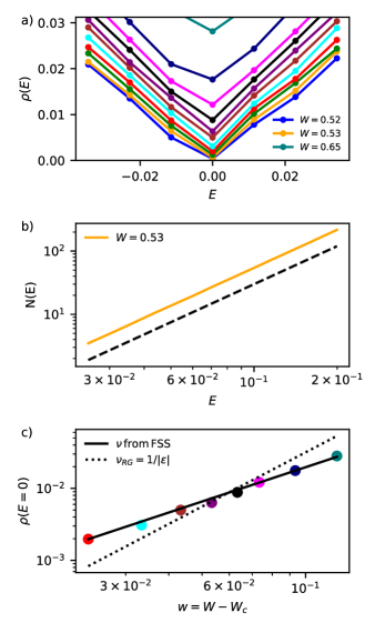
Figure 4: (a) Density of states $\rho(E,W)$ for $\alpha=0.4$ and $M=8001$ (dots). The solid lines are guides to the eye. (b) The integrated density of states close to criticality ($W=0.53$) is consistent with the scaling form $N(E)\propto E^{1/z}$ with $z=1/2$ (dashed line). (c) The zero-energy density of states (dots) follows the scaling $\rho(E=0,W>W_{c})\propto w^{(1-z)\nu}$ with $z=1/2$ and $\nu=3.163$ obtained from the finite-size scaling (solid line), but not with the analytical RG prediction $\nu_{RG}=1/|\varepsilon|$ (dotted line).

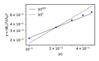
Figure 5: The dimensionless critical disorder strength $\gamma_{c}=W_{c}^{2}/\Lambda_{0}^{\varepsilon}$ obtained from the finite-size scaling of the Thouless conductance as a function of $\varepsilon$. The behaviour is consistent with the power-law fitting $\gamma_{c}\propto|\varepsilon|^{2/3}$ (solid line) and is distinct from the analytical prediction $\gamma_{c}\propto|\varepsilon|^{1}$ based on a one-loop perturbative RG calculation (dashed line).

VI Discussion and outlook

To summarise, in this paper we proposed and studied a one-dimensional model for the non-Anderson disorder-driven transitions. This model presents a rather convenient platform for investigating the non-Anderson criticality, as the system has a tunable small parameter $\varepsilon$ that controls the criticality. The model considered here exhibits the critical scaling of an observable (Thouless conductance) which does not vanish at the transition, unlike the density of states usually used in such studies, and thus allows for an accurate characterisation of the criticality. In our model, the energies of the states, for which the non-Anderson transition occurs, are not subject to renormalisation by disorder, which allows us to additionally increase the accuracy of the results.

Utilising the small parameter $\varepsilon$ allows us not only to study numerically the non-Anderson criticality within the expected range of applicability of the analytical perturbative RG approaches, but also to neglect possible non-perturbative rare-region effect Suslov (1994); Nandkishore et al. (2014); Note (1), exponentially suppressed by the large parameter $1/|\varepsilon|$ in the limit $\varepsilon\rightarrow 0$. This ensures the observability of the critical scaling in a parametrically large interval of disorder strengths and length scales.

Furthermore, the approach we develop here may be used to analyse the convergence of $\varepsilon$-expansions in interacting field theories similar to those describing the disordered high-dimensional systems.

Our data demonstrates the correlation-length critical exponent $1/\nu=3|\varepsilon|/2+{\cal O}(\varepsilon^{2})$ in the limit of small $\varepsilon$, which, contrary to the common expectation, is distinct from the prediction $1/\nu_{RG}=|\varepsilon|+{\cal O}(\varepsilon^{2})$ of the perturbative RG approach. Furthermore, the scaling of the dependence of the critical disorder strength on $|\varepsilon|$ is given by $\gamma_{c}\propto|\varepsilon|^{\frac{2}{3}}$, in accordance with the earlier study in Ref. de Moura et al., 2005 and in disagreement with the expectation $\gamma_{c}\propto|\varepsilon|$ from the perturbative RG analysis. At the same time, the numerical result for dynamical exponent, $z=\frac{1}{2}+{\cal O}(\varepsilon)$, agrees well with RG predictions. Similar agreement between the numerical values of the dynamical exponent $z$ and the one-loop RG results are observed for Weyl semimetals, while the results for the correlation-length exponent $\nu$ are controversial (see Ref. Syzranov and Radzihovsky, 2018 for a review).

We leave for future studies the origin of the disagreement between the numerical and the perturbative RG results for the correlation-length exponent in the limit of small $\varepsilon$. This disagreement may mean the breakdown of small-$\varepsilon$ expansions in the RG approaches or, for example, the existence of spontaneously generated operators in the field theories for non-Anderson transitions, which have been overlooked in the previous analytical studies of these transitions.

Such a possibility and the controversy around the values of the correlation-length exponents in Weyl semimetals call for a fresh analytical investigation of the non-Anderson criticality in these systems.

Assuming that the critical behaviour at the criticality is determined by one relevant coupling $\tilde{\gamma}$, our numerical results for the dependence of the critical disorder strength and the correlation-length exponent on $\varepsilon$ are consistent with the beta-function $\beta(\tilde{\gamma})=\varepsilon\tilde{\gamma}+(\tilde{\gamma})^{\frac{5}{3}}+\ldots$, where $\ldots$ stands for the terms of higher orders in $\tilde{\gamma}$. We leave for future studies the investigation of the possible nature of such variables.

VII Acknowledgements.

We thank Thomas Klein-Kvorning and Vlad Kozii for useful discussions. Our work has been financially supported by the German National Academy of Sciences Leopoldina through grant LPDS 2018-12 (BS) and the Hellman foundation (SS).

Appendix A Details of finite-size scaling and additional data

Here, we provide the details of the finite-size scaling data analysis, following Refs. Slevin and Ohtsuki, 1999, 2009, 2014. We consider the cases of power-law exponent $\alpha=\{0.45,0.4,0.35,0.3,0.25\}$, each for system sizes $L=2M$ with $M=\{451,675,1001,1501,2101\}$ and a range of disorder strengths $W$ in the vicinity of $W_{c}$, summarised in Table 1. For each $\alpha$ and each point $(W,L)$, we determine the median $\tilde{g}(W,L)$ of the conductance distribution and its uncertainty, $\sigma_{\tilde{g}}(W,L)$. We use between $\sim 10^{4}$ and $\sim 10^{5}$ disorder realizations, depending on the system size. The data is shown as symbols in Figs. 1b,c and 6. We then perform a least-squares fit

$$\tilde{g}_{\mathrm{fit}}(W,L)=a_{0}+\sum_{p=1}^{n_{p}}a_{p}\cdot\left(L^{1/\nu}\sum_{q=1}^{n_{q}}b_{q}\left[W-W_{c}\right]^{q}\right)^{p},$$ (9)

with $b_{1}=1$ for various orders $n_{p}$ and $n_{q}$ and obtain the quality of the fit in terms of

$$\chi^{2}/N=\frac{1}{N}\sum_{(W,L)}\frac{\left[\tilde{g}_{\mathrm{fit}}(W,L)-\tilde{g}(W,L)\right]^{2}}{\sigma_{\tilde{g}}^{2}(W,L)}$$ (10)

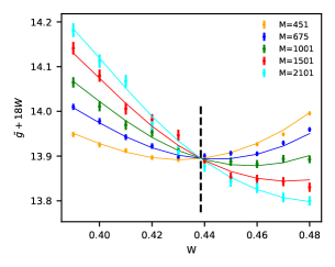
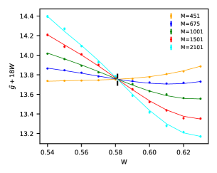
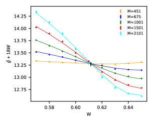
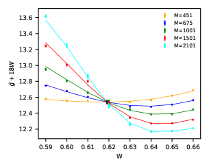
Figure 6: Finite-size scaling data as in Fig. 1a, but for $\alpha=0.45$, $0.35$, $0.3$, $0.25$ (left to right and top to bottom).

where $N$ is the total number of data points $(W,L)$ used in the fit. We increase $n_{p}$ and $n_{q}$ if this lowers the value of $\chi^{2}/N$ by more than 2% and the error of any fitting parameter does not exceed the parameter estimate in magnitude. We find that $n_{p}=4$ and $n_{q}=2$ yield the optimal fit in this sense. We verify also that the inclusion of possible irrelevant scaling variables Slevin and Ohtsuki (1999), corresponding to the replacement $a_{i}\rightarrow a_{i}\left(1+c_{i}L^{y}\right)$ with $y<0$ in Eq. (9), does not affect significantly the value of $\chi^{2}/N$ and does not lead to stable values of $y$, which allows us to neglect irrelevant scaling variables.

Each fitting procedure is repeated a hundred times with randomly chosen initial parameters. For the best fits with the lowest $\chi^{2}/N$, Table 1 reports the resulting parameters $\nu$, $W_{c}$, their error estimates and $\chi^{2}/N$. The best fits are shown by solid lines in Figs. 1a and 6. We find that removing the largest or smallest length data set ($M=451$ or $M=2101$) from the fitting procedure does produce consistent results with the estimates for $\nu$ and $W_{c}$ within the previous error bars (data not shown).

$\alpha$	$|\epsilon|$	$W$	$M=L/2a$	$N$	$\chi^{2}/N$	$\nu$	$W_{c}$
0.45	0.1	0.39,0.40,…,0.48	451,675,1001,1501,2101	50	0.920	6.196$\pm$0.171	0.4385$\pm$0.0010
0.40	0.2	0.49,0.495…,0.56	451,675,1001,1501,2101	75	0.797	$3.163\pm 0.041$	0.5267$\pm$0.0004
0.35	0.3	0.54,0.55,…,0.63	451,675,1001,1501,2101	50	0.915	2.111$\pm$0.021	0.5812$\pm$0.0003
0.30	0.4	0.57,0.58,…,0.65	451,675,1001,1501,2101	45	1.277	1.719$\pm$0.017	0.6116$\pm$0.0003
0.25	0.5	0.59,0.60,…,0.66	451,675,1001,1501,2101	40	1.588	1.532$\pm$0.022	0.6191$\pm$0.0003

Table 1: Details for the finite-size scaling: The left two columns specify the value of $\epsilon=2\alpha-1$, the third and fourth the disorder strength $W$ and system size $L=2M$, respectively. The total number of data points $(W,L)$ is denoted by $N$. The right part of the table reports the $\chi^{2}/N$ value for the best fit along with its estimate for the critical exponent $\nu$ and the critical disorder strength $W_{c}$. The error (denoted after the $\pm$ symbol) is one standard deviation. The respective plots can be found in Fig. 1a ($\alpha=0.4$) and Fig. 6 ($\alpha=0.45$, $0.35$, $0.3$, $0.25$).

Appendix B Perturbative renormalisation-group analysis

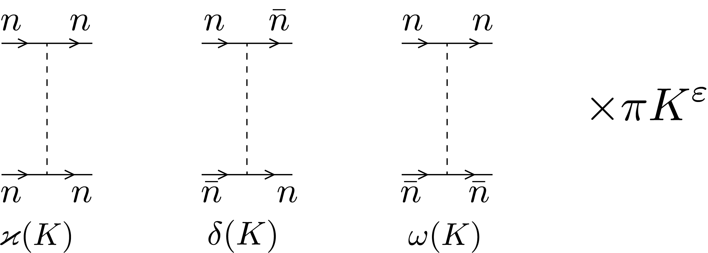
Figure 7: Elements of the diagrammatic technique (impurity lines) used to compute disorder-averaged observables in a model with two nodes described by the Hamiltonian (3). The coupling constants $\varkappa(K)$, $\delta(K)$ and $\omega(K)$ depend on the ultraviolet momentum cutoff $K$.

In this section, we provide a detailed one-loop RG analysis for a model with the two-node quasiparticle dispersion (3) in the presence of random potential with a short correlation length. The wavevector $k$ of the quasiparticles we consider is measured from either of the nodes $n=1,2$ and is exceeded significantly by the inverse characteristic correlation length of the random potential. Disorder-averaged observables in this systems may be described by a supersymmetric Efetov (1999) field theory with the action

$${\cal L}= -i\sum\limits_{n=1,2}\left\{\int\bar{\psi}_{n}\left[-k^{\alpha}\operatorname{sign}k+i0\Lambda\right]\psi_{n}\,dx\right.$$

$$\left.+\frac{1}{2}\varkappa(K)K^{\varepsilon}\int\left(\bar{\psi}_{n}\psi_{n}\right)^{2}dx+\frac{1}{2}\delta(K)K^{\varepsilon}\int\left(\bar{\psi}_{n}\psi_{\bar{n}}\right)\left(\bar{\psi}_{\bar{n}}\psi_{n}\right)dx+\frac{1}{2}\omega(K)K^{\varepsilon}\int\left(\bar{\psi}_{n}\psi_{n}\right)\left(\bar{\psi}_{\bar{n}}\psi_{\bar{n}}\right)dx\right\},$$ (11)

where $\bar{\psi}_{n}(x)$ and $\psi_{n}(x)$ are the supervectors in the $BF\otimes AR$ (boson-fermion$\otimes$advanced-retarded) space describing the quasiparticles near node $n$; $\bar{n}$ is our convention for the node other than $n$, i.e. $\bar{1}=2$ and $\bar{2}=1$; $\Lambda=\left({\hat{\sigma}}_{z}\right)_{AR}$; $k=-i\partial_{x}$ is the momentum operator; $K$ is the ultraviolet momentum cutoff. The coupling constants $\varkappa(K)$, $\delta(K)$ and $\omega(K)$ which characterise scattering processes shown in Fig. 7 flow under renormalisation.

The renormalisation procedure involves repeatedly integrating out particle modes with highest momenta, starting at the ultraviolet momentum cutoff $K=K_{0}$ and correcting the action of the low-momentum modes to account for the effect of the higher momenta. Upon renormalisation, the action (11) reproduces itself with flowing couplings $\varkappa(K)$, $\delta(K)$ and $\omega(K)$. The perturbative one-loop corrections to each of the three coupling constants are shown in Fig. 8. The momenta, which we integrate out, are away from the poles of the Green’s functions and, therefore, both advanced and retarded Green’s functions may be approximated as $G_{1,2}(p)\approx\mp\frac{\operatorname{sign}p}{p^{\alpha}}$.

The flows of the coupling constants $\varkappa(K)$, $\delta(K)$ and $\omega(K)$ may be represented in the form

$$\partial_{l}\varkappa= \beta_{\varkappa}(\varkappa,\delta,\omega),$$ (12a)

$$\partial_{l}\delta= \beta_{\delta}(\varkappa,\delta,\omega),$$ (12b)

$$\partial_{l}\omega= \beta_{\omega}(\varkappa,\delta,\omega),$$ (12c)

where the beta-functions

$$\beta_{\varkappa}(\varkappa,\delta,\omega)= \varepsilon\varkappa+2\varkappa^{2}+2\omega\delta+\delta^{2}+\ldots,$$ (13a)

$$\beta_{\delta}(\varkappa,\delta,\omega)= \varepsilon\delta+2\delta\varkappa+\ldots,$$ (13b)

$$\beta_{\omega}(\varkappa,\delta,\omega)= \varepsilon\omega+2\delta\varkappa+2\varkappa\omega+\delta^{2}+\ldots.$$ (13c)

are given, to the one-loop order, by the sum of the diagrams in Fig. (8) and $\ldots$ are higher-order terms in the coupling constants.

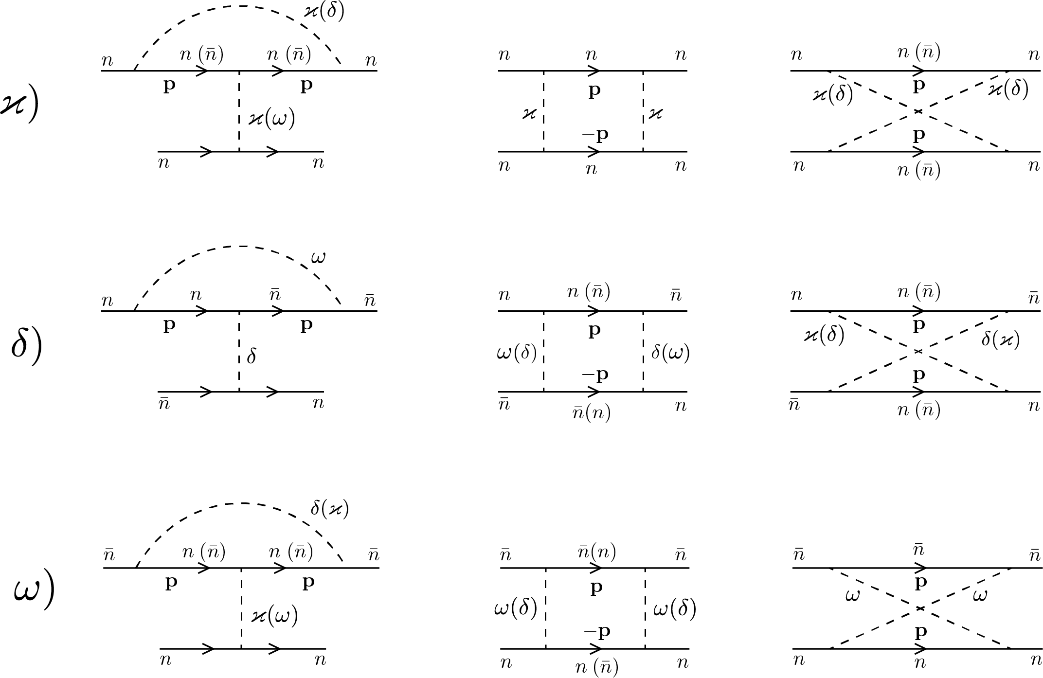
Figure 8: Diagrams (in units of $\pi^{2}K^{2\varepsilon}$) contributing to the one-loop renormalisations of the coupling constants $\varkappa$, $\delta$ and $\omega$. Symbols in parentheses indicate alternative nodes or types of impurity lines. For each shown “mushroom” diagram, there exists one equivalent diagram with an impurity line connecting two points on the bottom particle propagator in place of the top propagator.

The fixed points of the flow are determined by the conditions $\beta_{\varkappa}(\varkappa^{*},\delta^{*},\omega^{*})=\beta_{\delta}(\varkappa^{*},\delta^{*},\omega^{*})=\beta_{\omega}(\varkappa^{*},\delta^{*},\omega^{*})=0$. Utilising Eq. (13b), this requires that either $\delta^{*}=-\frac{\varepsilon}{2}$ or $\delta^{*}=0$. Using that $\varkappa(K)=\omega(K)$ for the initial conditions for the flow under consideration and the form of the beta-functions $\beta_{\delta}$ and $\beta_{\omega}$ given by Eqs. (13a) and (13c), we obtain the values of the coupling constants at two fixed points (to the leading order in $|\varepsilon|$): 1) $\delta^{*}=0$, $\varkappa^{*}=\omega^{*}=-\frac{\varepsilon}{2}$ and 2) $\delta^{*}=\varepsilon$, $\varkappa^{*}=\omega^{*}=-\frac{\varepsilon}{2}$. We note that for the model under consideration all couplings remain positive under renormalisation and, therefore, the second fixed point is unachievable as it corresponds to a negative coupling $\delta$.

The correlation-length exponents $\nu$ at the transition are given by the inverse eigenvalues of the Jacobian $\frac{\partial\left(\beta_{\varkappa},\beta_{\delta},\beta_{\omega}\right)}{\partial\left(\varkappa,\delta,\omega\right)}$. Utilising Eqs. (13a)-(13c), we obtain at the first fixed point

$$\frac{\partial\left(\beta_{\varkappa},\beta_{\delta},\beta_{\omega}\right)}{\partial\left(\varkappa,\delta,\omega\right)}(\varkappa^{*},\delta^{*},\omega^{*})=\left(\begin{array}[]{ccc}-\varepsilon&-\varepsilon&0\\ 0&0&0\\ -\varepsilon&-\varepsilon&0\end{array}\right)+{\cal O}\left(\varepsilon^{2}\right).$$ (17)

The Jacobian (17) gives the correlation-length exponent $1/\nu_{RG}=-\varepsilon$.

In addition to the above analysis of the fixed points, we verify the correlation-lenght exponent by solving the RG equations (12a) – (13c) numerically with the initial conditions $\kappa(K_{0})=\delta(K_{0})=\omega(K_{0})=\gamma_{0}$ corresponding to the short-range-correlated random potential considered in this paper. First, we identify the critical disorder strength $\gamma_{c}$ by varying $\gamma$ for fixed $\varepsilon<0$ and detecting the value of $\gamma$ at which the flows become unstable. Next, we determine the correlation-length exponent by solving numerically the RG equations for the supercritical disorder strength $\gamma_{0}=\gamma_{c}+\Delta$ with a small $\Delta>0$, where we vary $\Delta$ such that it is an order of magnitude larger than the uncertainty of $\gamma_{c}$ and an order of magnitude smaller than $\gamma_{c}$. We find the RG time $l=\tilde{l}$ where the flow of $\kappa(l)=\omega(l)$ diverges and the numerical solution breaks down. Due to the extreme sharpness of the divergence, this agrees with the more common requirement $\kappa(\tilde{l})=\omega(\tilde{l})=C$ with $C=\mathcal{O}(1)$. The RG time $\tilde{l}$ is related to the emergent correlation length $\xi$ as $\tilde{l}\sim\mathrm{log}\xi$. In Fig. 9, we confirm the scaling form $\xi\propto\Delta^{-\nu}$ by plotting $\mathrm{log}(\xi)$ versus $\mathrm{log}(\Delta)$. Indeed, the data points for $\varepsilon=-0.1$ (blue) and $\varepsilon=-0.2$ (red) lie on straight lines with slopes $-\nu_{RG}=-1/|\varepsilon|$, confirming the results from the fixed-point analysis in the previous paragraph. In addition, we confirm also that $\gamma_{c}\propto|\varepsilon|$.

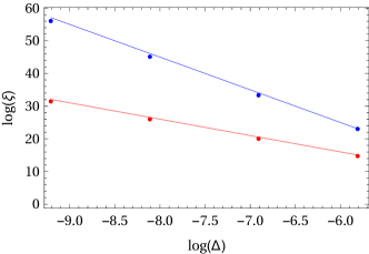
Figure 9: Verification of the scaling form $\xi\propto\Delta^{-\nu}$ for $\Delta=\gamma_{0}-\gamma_{c}$ based on the numerical solution of the flow equations (12a) – (13c). The numerically extracted correlation length data (dots) for $\varepsilon=-0.1$ (blue) and $\varepsilon=-0.2$ (red) lie on straigth lines with the slope $-\nu_{RG}=-1/|\varepsilon|$.

References

- Efetov (1999) K. B. Efetov, Supersymetry in Disorder and Chaos (Cambridge University Press, New York, 1999).
- Kamenev (2011) A. Kamenev, Field Theory of Non-Equilibrium Systems (Cambridge Univ. Press, Cambridge, 2011).
- Belitz and Kirkpatrick (1994) D. Belitz and T. R. Kirkpatrick, “The anderson-mott transition,” Rev. Mod. Phys. 66, 261–380 (1994).
- Dasgupta and Ma (1980) Chandan Dasgupta and Shang-keng Ma, “Low-temperature properties of the random heisenberg antiferromagnetic chain,” Phys. Rev. B 22, 1305–1319 (1980).
- Fisher (1994) Daniel S. Fisher, “Random antiferromagnetic quantum spin chains,” Phys. Rev. B 50, 3799–3821 (1994).
- Altman et al. (2004) Ehud Altman, Yariv Kafri, Anatoli Polkovnikov, and Gil Refael, “Phase transition in a system of one-dimensional bosons with strong disorder,” Phys. Rev. Lett. 93, 150402 (2004).
- Levitov (1990) L. S. Levitov, “Delocalization of vibrational modes caused by electric dipole interaction,” Phys. Rev. Lett. 64, 547–550 (1990).
- Levitov (1989) L. S. Levitov, “Absence of localization of vibrational modes due to dipole-dipole interaction,” Europhys. Lett. 9, 83–86 (1989).
- Burin (2006) A. L. Burin, “Energy delocalization in strongly disordered systems induced by the long-range many-body interaction,” eprint arXiv:cond-mat/0611387 (2006).
- Cardy (1996) J. Cardy, Scaling and Renormalization in Statistical Physics, edited by P. Goddard and J. Yeomans (Cambridge University Press, Cambridge, 1996).
- Mirlin (2000) A. D. Mirlin, “Statistics of energy levels and eigenfunctions in disordered systems,” Phys. Rep. 326, 259–382 (2000).
- Mirlin and Evers (2000) A. D. Mirlin and F. Evers, “Multifractality and critical fluctuations at the anderson transition,” Phys. Rev. B 62, 7920–7933 (2000).
- Syzranov and Radzihovsky (2018) S. V. Syzranov and L. Radzihovsky, “High-dimensional disorder-driven phenomena in weyl semimetals, semiconductors, and related systems,” Annu. Rev. Cond. Mat. Phys. 9, 33–58 (2018).
- Note (1) It has recently been debated (for example, in Refs. \rev@citealpnumNandkishore:rare,Sbierski:WeylVector,Mafia:rare,Gurarie:AvoidedCriticality,BuchholdAltland:rare,BuchholdAltland:rare2), in the context of Weyl semimetals, if these transitions survive non-perturbative rare-region effects or get converted to sharp crossovers. We do not distinguish between true phase transition and sharp crossovers in this paper, provided the non-Anderson critical scaling exists in a parametrically large interval of lengths.
- Fradkin (1986a) Eduardo Fradkin, “Critical behavior of disordered degenerate semiconductors. i. models, symmetries, and formalism,” Phys. Rev. B 33, 3257–3262 (1986a).
- Fradkin (1986b) Eduardo Fradkin, “Critical behavior of disordered degenerate semiconductors. ii. spectrum and transport properties in mean-field theory,” Phys. Rev. B 33, 3263–3268 (1986b).
- Syzranov et al. (2015a) S. V. Syzranov, L. Radzihovsky, and V. Gurarie, “Critical transport in weakly disordered semiconductors and semimetals,” Phys. Rev. Lett. 114, 166601 (2015a).
- Syzranov and Gurarie (2019) S. V. Syzranov and V. Gurarie, “Duality between disordered nodal semimetals and systems with power-law hopping,” Phys. Rev. Research 1, 032035 (2019).
- Richerme et al. (2014) Philip Richerme, Zhe-Xuan Gong, Aaron Lee, Crystal Senko, Jacob Smith, Michael Foss-Feig, Spyridon Michalakis, Alexey V. Gorshkov, and Christopher Monroe, “Non-local propagation of correlations in quantum systems with long-range interactions,” Nature Lett. 511, 198–201 (2014).
- Islam et al. (2013) R. Islam, C. Senko, W. C. Campbell, S. Korenblit, J. Smith, A. Lee, E. E. Edwards, C.-C. J. Wang, J. K. Freericks, and C. Monroe, “Emergence and frustration of magnetism with variable-range interactions in a quantum simulator,” Science 340, 583–587 (2013).
- Jurcevic et al. (2014) P. Jurcevic, B. P. Lanyon, P. Hauke, C. Hempel, P. Zoller, R. Blatt, and C. F. Roos, “Quasiparticle engineering and entanglement propagation in a quantum many-body system,” Nature 511, 202–205 (2014).
- Jurcevic et al. (2015) P. Jurcevic, P. Hauke, C. Maier, C. Hempel, B. P. Lanyon, R. Blatt, and C. F. Roos, “Spectroscopy of interacting quasiparticles in trapped ions,” Phys. Rev. Lett. 115, 100501 (2015).
- Rodríguez et al. (2000) A Rodríguez, V A Malyshev, and F Domínguez-Adame, “Quantum diffusion and lack of universal one-parameter scaling in one-dimensional disordered lattices with long-range coupling,” Journal of Physics A: Mathematical and General 33, L161–L166 (2000).
- Rodríguez et al. (2003) A. Rodríguez, V. A. Malyshev, G. Sierra, M. A. Martín-Delgado, J. Rodríguez-Laguna, and F. Domínguez-Adame, “Anderson transition in low-dimensional disordered systems driven by long-range nonrandom hopping,” Phys. Rev. Lett. 90, 027404 (2003).
- Malyshev et al. (2004) A. V. Malyshev, V. A. Malyshev, and F. Domínguez-Adame, “Monitoring the localization-delocalization transition within a one-dimensional model with nonrandom long-range interaction,” Phys. Rev. B 70, 172202 (2004).
- de Moura et al. (2005) F. A. B. F. de Moura, A. V. Malyshev, M. L. Lyra, V. A. Malyshev, and F. Domínguez-Adame, “Localization properties of a one-dimensional tight-binding model with nonrandom long-range intersite interactions,” Phys. Rev. B 71, 174203 (2005).
- Xiong and Zhang (2003) S. J. Xiong and G.P. Zhang, “Scaling behavior of the metal-insulator transition in one-dimensional disordered systems with long-range hopping,” Phys. Rev. B 68, 1–4 (2003).
- Gärttner et al. (2015) M. Gärttner, S. V. Syzranov, Ana Maria Rey, V. Gurarie, and L. Radzihovsky, “Disorder-driven transition in a chain with power-law hopping,” Phys. Rev. B 92, 041406(R) (2015).
- Tikhonov and Feigel’man (2020) Konstantin Tikhonov and Mikhail Feigel’man, “Strange metal state near quantum superconductor-metal transition in thin films,” arXiv e-prints , arXiv:2002.08107 (2020).
- Suslov (1994) I. M. Suslov, “Density of states near an anderson transition in four-dimensional space: Lattice mode,” Sov. Phys. JETP 79, 307–320 (1994).
- Nandkishore et al. (2014) Rahul Nandkishore, David A. Huse, and S. L. Sondhi, “Rare region effects dominate weakly disordered 3d dirac points,” Phys. Rev. B 89, 245110 (2014).
- Syzranov et al. (2015b) S. V. Syzranov, V. Gurarie, and L. Radzihovsky, “Unconventional localisation transition in high dimensions,” Phys. Rev. B 91, 035133 (2015b).
- Shindou and Murakami (2009) Ryuichi Shindou and Shuichi Murakami, “Effects of disorder in three-dimensional quantum spin hall systems,” Phys. Rev. B 79, 045321 (2009).
- Goswami and Chakravarty (2011) Pallab Goswami and Sudip Chakravarty, “Quantum criticality between topological and band insulators in dimensions,” Phys. Rev. Lett. 107, 196803 (2011).
- Ryu and Nomura (2012) Shinsei Ryu and Kentaro Nomura, “Disorder-induced quantum phase transitions in three-dimensional topological insulators and superconductors,” Phys. Rev. B 85, 155138 (2012).
- Kobayashi et al. (2014) Koji Kobayashi, Tomi Ohtsuki, Ken-Ichiro Imura, and Igor F. Herbut, “Density of states scaling at the semimetal to metal transition in three dimensional topological insulators,” Phys. Rev. Lett. 112, 016402 (2014).
- Louvet et al. (2016) T. Louvet, D. Carpentier, and A. A. Fedorenko, “On the disorder-driven quantum transition in three-dimensional relativistic metals,” Phys. Rev. B 94, 220201 (2016).
- Roy et al. (2018) Bitan Roy, Robert-Jan Slager, and Vladimir Juričić, “Global phase diagram of a dirty weyl liquid and emergent superuniversality,” Phys. Rev. X 8, 031076 (2018).
- Syzranov et al. (2016) S. V. Syzranov, P. M. Ostrovsky, V. Gurarie, and L. Radzihovsky, “Critical exponents at the unconventional disorder-driven transition in a weyl semimetal,” Phys. Rev. B 93, 155113 (2016).
- Pixley et al. (2016) J. H. Pixley, D. A. Huse, and S. Das Sarma, “Rare-Region-Induced Avoided Quantum Criticality in Disordered Three-Dimensional Dirac and Weyl Semimetals,” Physical Review X 6, 021042 (2016).
- Sbierski et al. (2015) Björn Sbierski, Emil J. Bergholtz, and Piet W. Brouwer, “Quantum critical exponents for a disordered three-dimensional weyl node,” Phys. Rev. B 92, 115145 (2015).
- Bera et al. (2016) Soumya Bera, Jay D. Sau, and Bitan Roy, “Dirty weyl semimetals: Stability, phase transition, and quantum criticality,” Phys. Rev. B 93, 201302 (2016).
- Liu et al. (2016) Shang Liu, Tomi Ohtsuki, and Ryuichi Shindou, “Effect of disorder in three dimensional layered chern insulator,” Phys. Rev. Lett. 116, 066401 (2016).
- Balog et al. (2018) Ivan Balog, David Carpentier, and Andrei A. Fedorenko, “Disorder-Driven Quantum Transition in Relativistic Semimetals: Functional Renormalization via the Porous Medium Equation,” Phys. Rev. Lett. 121, 166402 (2018), 1710.07932 .
- Pixley et al. (2015) J. H. Pixley, Pallab Goswami, and S. Das Sarma, “Anderson Localization and the Quantum Phase Diagram of Three Dimensional Disordered Dirac Semimetals,” Phys. Rev. Lett. 115, 076601 (2015).
- Klier et al. (2019) J. Klier, I. V. Gornyi, and A. D. Mirlin, “From weak to strong disorder in Weyl semimetals: Self-consistent Born approximation,” Phys. Rev. B 100, 125160 (2019).
- Edwards and Thouless (1972) J T Edwards and D J Thouless, “Numerical studies of localization in disordered systems,” Journal of Physics C: Solid State Physics 5, 807–820 (1972).
- Thouless (1974) D. J. Thouless, “Electrons in disordered systems and the theory of localization,” Phys. Rep. 13, 93 (1974).
- Braun et al. (1997) D Braun, E Hofstetter, A Mackinnon, and G Montambaux, “Level curvatures and conductances: A numerical study of the Thouless relation,” Phys. Rev. B 55, 7557 (1997).
- Slevin and Ohtsuki (1999) Keith Slevin and Tomi Ohtsuki, “Corrections to scaling at the Anderson transition,” Phys. Rev. Lett. 82, 382 (1999).
- Slevin and Ohtsuki (2009) Keith Slevin and Tomi Ohtsuki, “Critical exponent for the quantum Hall transition,” Phys. Rev. B 80, 041304 (2009).
- Slevin and Ohtsuki (2014) Keith Slevin and Tomi Ohtsuki, “Critical exponent for the Anderson transition in the three-dimensional orthogonal universality class,” New J. Phys. 16, 1–20 (2014).
- Buchhold et al. (2018a) Michael Buchhold, Sebastian Diehl, and Alexander Altland, “Nodal points of weyl semimetals survive the presence of moderate disorder,” Phys. Rev. B 98, 205134 (2018a).
- Sbierski et al. (2016) B. Sbierski, K. S. C. Decker, and P. W. Brouwer, “Weyl node with random vector potential,” Phys. Rev. B 94, 220202 (2016).
- Pixley et al. (2017) J. H. Pixley, Y.-Z. Chou, P. Goswami, D. A. Huse, R. Nandkishore, L. Radzihovsky, and S. Das Sarma, “Single-particle excitations in disordered Weyl fluids,” Phys. Rev. B 95, 235101 (2017).
- Gurarie (2017) V. Gurarie, “Theory of avoided criticality in quantum motion in a random potential in high dimensions,” Phys. Rev. B 96, 014205 (2017).
- Buchhold et al. (2018b) Michael Buchhold, Sebastian Diehl, and Alexander Altland, “Vanishing density of states in weakly disordered weyl semimetals,” Phys. Rev. Lett. 121, 215301 (2018b).