Random-Order Models

Abstract

This chapter introduces the random-order model in online algorithms. In this model, the input is chosen by an adversary, then randomly permuted before being presented to the algorithm. This reshuffling often weakens the power of the adversary and allows for improved algorithmic guarantees. We show such improvements for two broad classes of problems: packing problems where we must pick a constrained set of items to maximize total value, and covering problems where we must satisfy given requirements at minimum total cost. We also discuss how random-order model relates to other stochastic models used for non-worst-case competitive analysis.  

1 Motivation: Picking a Large Element

Suppose we want to pick the maximum of a collection of $n$ numbers. At the beginning, we know this cardinality $n$, but nothing about the range of numbers to arrive. We are then presented distinct non-negative real numbers $v_{1},v_{2},\ldots,v_{n}$ one by one; upon seeing a number $v_{i}$, we must either immediately pick it, or discard it forever. We can pick at most one number. The goal is to maximize the expected value of the number we pick, where the expectation is over any randomness in our algorithm. We want this expected value to be close to the maximum value $v_{\max}:=\max_{i\in\{1,2,\ldots,n\}}v_{i}$. Formally, we want to minimize the competitive ratio, which is defined as the ratio of $v_{\max}$ to our expected value. Note that this maximum $v_{\max}$ is independent of the order in which the elements are presented, and is unknown to our algorithm until all the numbers have been revealed.

If we use a deterministic algorithm, our value can be arbitrarily smaller than $v_{\max}$, even for $n=2$. Say the first number $v_{1}=1$. If our deterministic algorithm picks $v_{1}$, the adversary can present $v_{2}=M\gg 1$; if it does not, the adversary can present $v_{2}=\nicefrac{{1}}{{M}}\ll 1$. Either way, the adversary can make the competitive ratio as bad as it wants by making $M$ large.

Using a randomized algorithm helps only a little: a naïve randomized strategy is to select a uniformly random position $i\in\{1,\ldots,n\}$ up-front and pick the $i^{th}$ number $v_{i}$. Since we pick each number with probability $1/n$, the expected value is $\sum_{i}v_{i}/n\geq v_{\max}/n$. This turns out to be the best we can do, as long the input sequence is controlled by an adversary and the maximum value is much larger than the others. Indeed, one strategy for the adversary is to choose a uniformly random index $j$, and present the request sequence $1,M,M^{2},\ldots,M^{j},0,0,\ldots,0$—a rapidly ascending chain of $j$ numbers followed by worthless numbers. If $M$ is very large, any good algorithm must pick the last number in the ascending chain upon seeing it. But this is tantamount to guessing $j$, and random guessing is the best an algorithm can do. (This intuition can be made formal using Yao’s minimax lemma.)

These bad examples show that the problem is hard for two reasons: the first reason being the large range of the numbers involved, and the second being the adversary’s ability to carefully design these difficult sequences. Consider the following way to mitigate the latter effect: what if the adversary chooses the $n$ numbers, but then the numbers are shuffled and presented to the algorithm in a uniformly random order? This random-order version of the problem above is commonly known as the secretary problem: the goal is to hire the best secretary (or at least a fairly good one) if the candidates for the job appear in a random order.

Somewhat surprisingly, randomly shuffling the numbers changes the complexity of the problem drastically. Here is the elegant $50\%$-algorithm:

  

1. Reject the first $n/2$ numbers, and then

2. Pick the first number after that which is bigger than all the previous numbers (if any).

  

Theorem 1.1.

The 50%-algorithm gets an expected value of at least $v_{\max}/4$.

• Assume for simplicity all numbers are distinct. The algorithm definitely picks $v_{\max}$ if the highest number is in the second half of the random order (which happens with probability $\nicefrac{{1}}{{2}}$), and also the second-highest number is in the first half (which, conditioned on the first event, happens with probability at least $\nicefrac{{1}}{{2}}$, the two events being positively correlated). Hence, we get an expected value of at least $v_{\max}/4$. (We get a stronger guarantee: we pick the highest number $v_{\max}$ itself with probability at least $\nicefrac{{1}}{{4}}$, but we will not explore this expected-value-versus-probability direction any further.)  

1.1 The Model and a Discussion

The secretary problem, with the lower bounds in the worst-case setting and an elegant algorithm for the random-order model, highlights the fact that sequential decision-making problems are often hard in the worst-case not merely because the underlying set of requests is hard, but also because these requests are carefully woven into a difficult-to-solve sequence. In many situations where there is no adversary, it may be reasonable to assume that the ordering of the requests is benign, which leads us to the random-order model. Indeed, one can view this as a semi-random model from Chapter 9, where the input is first chosen by an adversary and then randomly perturbed before being given to the algorithm.

Let us review the competitive analysis model for worst-case analysis of online algorithms (also discussed in Chapter 24). Here, the adversary chooses a sequence of requests and present them to the algorithm one by one. The algorithm must take actions to serve a request before seeing the next request, and it cannot change past decisions. The actions have rewards, say, and the competitive ratio is the optimal reward for the sequence (in hindsight) divided by the algorithm’s reward. (For problems where we seek to minimize costs instead of maximize rewards, the competitive ratio is the algorithm’s cost divided by the optimal cost.) Since the algorithm can never out-perform the optimal choice, the competitive ratio is always at least $1$.

Now given any online problem, the random-order model (henceforth the RO model) considers the setting where the adversary first chooses a set $S$ of requests (and not a sequence). The elements of this set are then presented to the algorithm in a uniformly random order. Formally, given a set $S=\{r_{1},r_{2},\ldots,r_{n}\}$ of $n=|S|$ requests, we imagine nature drawing a uniformly random permutation $\pi$ of $\{1,\ldots,n\}$, and then defining the input sequence to be $r_{\pi(1)},r_{\pi(2)},\cdots,r_{\pi(n)}$. As before, the online algorithm sees these requests one by one, and has to perform its irrevocable actions for $r_{\pi(i)}$ before seeing $r_{\pi(i+1)}$. The length $n$ of the input sequence may also be revealed to the algorithm at the beginning, depending on the problem. The competitive ratio (for maximization problems) is defined as the ratio between the optimum value for $S$ and the expected value of the algorithm, where the expectation is now taken over both the randomness of the reshuffle $\pi$ and that of the algorithm. (Again, we use the convention that the competitive ratio is at least one, and hence have to flip the ratio for minimization problems.)

A strength of the RO model is its simplicity, and that it captures other commonly considered stochastic input models. Indeed, since the RO model does not assume the algorithm has any prior knowledge of the underlying set of requests (except perhaps the cardinality $n$), it captures situations where the input sequence consists of independent and identically distributed (i.i.d.) random draws from some fixed and unknown distribution. Reasoning about the RO model avoids over-fitting the algorithm to any particular properties of the distribution, and makes the algorithms more general and robust by design.

Another motivation for the RO model is aesthetic and pragmatic: the simplicity of the model makes it a good starting point for designing algorithms. If we want to develop an online algorithm (or even an offline one) for some algorithmic task, a good step is to first solve it in the RO model, and then extend the result to the worst-case setting. This can be useful either way: in the best case, we may succeed in getting an algorithm for the worst-case setting using the insights developed in the RO model. Else the extension may be difficult, but still we know a good algorithm under the (mild?) assumption of random-order arrivals.

Of course, the assumption of uniform random orderings may be unreasonable in some settings, especially if the algorithm performs poorly when the random-order assumption is violated. There have been attempts to refine the model to require less randomness from the input stream, while still getting better-than-worst-case performance. We discuss some of these in §5.2, but much remains to be done.

1.2 Roadmap

In §2 we discuss an optimal algorithm for the secretary problem. In §3 we give algorithms to choose multiple items instead of just a single one, and other maximization packing problems. In §4 we discuss minimization problems. In §5 we present some specializations and extensions of the RO model.

2 The Secretary Problem

We saw the $50\%$ algorithm based on the idea of using the first half of the random order sequence to compute a threshold that weeds out “low” values. This idea of choosing a good threshold will be a recurring one in this chapter. The choice of waiting for half of the sequence was for simplicity: a right choice is to wait for $\nicefrac{{1}}{{e}}\approx 37\%$ fraction, which gives us the $37\%$-algorithm:

  

1. Reject the first $n/e$ numbers, and then

2. Pick the first number after that (if any) which is bigger than all the previous numbers.

  

(Although $n/e$ is not an integer, rounding it to the nearest integer does not impact the guarantees substantively.) Call a number a prefix-maximum if it is the largest among the numbers revealed before it. Notice being the maximum is a property of just the set of numbers, whereas being a prefix-maximum is a property of the random sequence and the current position. A wait-and-pick algorithm is one that rejects the first $m$ numbers, and then picks the first prefix-maximum number.

Theorem 2.1.

As $n\rightarrow\infty$, the 37%-algorithm picks the highest number with probability at least $\nicefrac{{1}}{{e}}$. Hence, it gets expected value at least $v_{\max}/e$. Moreover, $n/e$ is the optimal choice of $m$ among all wait-and-pick algorithms.

• If we pick the first prefix-maximum after rejecting the first $m$ numbers, the probability we pick the maximum is

  $$\sum_{t=m+1}^{n}\Pr[v_{t}\text{ is max}]\cdot\Pr[\text{max among first $t-1$ numbers falls in first $m$ positions}]$$

  $$\stackrel{{\scriptstyle(\star)}}{{=}}\sum_{t=m+1}^{n}\frac{1}{n}\cdot\frac{m}{t-1}\quad=\quad\frac{m}{n}\big{(}H_{n-1}-H_{m-1}\big{)},$$

  where $H_{k}=1+\frac{1}{2}+\frac{1}{3}+\ldots+\frac{1}{k}$ is the $k^{th}$ harmonic number. The equality $(\star)$ uses the uniform random order. Now using the approximation $H_{k}\approx\ln k+0.57$ for large $k$, we get the probability of picking the maximum is about $\frac{m}{n}\ln\frac{n-1}{m-1}$ when $m,n$ are large. This quantity has a maximum value of $1/e$ if we choose $m=n/e$.  

Next we show we can replace any strategy (in a comparison-based model) with a wait-and-pick strategy without decreasing the probability of picking the maximum.

Theorem 2.2.

The strategy that maximizes the probability of picking the highest number can be assumed to be a wait-and-pick strategy.

• Think of yourself as a player trying to maximize the probability of picking the maximum number. Clearly, you should reject the next number $v_{i}$ if it is not prefix-maximum. Otherwise, you should pick $v_{i}$ only if it is prefix-maximum and the probability of $v_{i}$ being the maximum is more than the probability of you picking the maximum in the remaining sequence. Let us calculate these probabilities.

  We use Pmax to abbreviate “prefix-maximum”. For position $i\in\{1,\ldots,n\}$, define

  $$f(i) =\Pr[v_{i}\text{ is max}\mid v_{i}\text{ is Pmax}]\stackrel{{\scriptstyle(\star)}}{{=}}\frac{\Pr[v_{i}\text{ is max}]}{\Pr[v_{i}\text{ is Pmax}]}\stackrel{{\scriptstyle(\star\star)}}{{=}}\frac{1/n}{1/i}=\frac{i}{n},$$

  where equality $(\star)$ uses that the maximum is also a prefix-maximum, and $(\star\star)$ uses the uniform random ordering. Note that $f(i)$ increases with $i$.

  Now consider a problem where the numbers are again being revealed in a random order but we must reject the first $i$ numbers. The goal is to still maximize the probability of picking the highest of the $n$ numbers. Let $g(i)$ denote the probability that the optimal strategy for this problem picks the global maximum.

  The function $g(i)$ must be a non-increasing function of $i$, else we could just ignore the $(i+1)^{st}$ number and set $g(i)$ to mimic the strategy for $g(i+1)$. Moreover, $f(i)$ is increasing. So from the discussion above, you should not pick a prefix-maximum number at any position $i$ where $f(i)<g(i)$ since you can do better on the suffix. Moreover, when $f(i)\geq g(i)$, you should pick $v_{i}$ if it is prefix-maximum, since it is worse to wait. Therefore, the approach of waiting until $f$ becomes greater than $g$ and thereafter picking the first prefix-maximum is an optimal strategy.  

Theorems 2.1 and 2.2 imply for $n\to\infty$ that no algorithm can pick the maximum with probability more than $1/e$. Since we placed no bounds on the number magnitudes, this can also be used to show that for any $\varepsilon>0$, there exist an $n$ and numbers $\{v_{i}\}_{i\in\{1,\ldots,n\}}$ where every algorithm has expected value at most $(1/e+\varepsilon)\cdot\max_{i}v_{i}$.

3 Multiple-Secretary and Other Maximization Problems

We now extend our insights from the single-item case to settings where we can pick multiple items. Each item has a value, and we have constraints on what we can pick (e.g., we can pick at most $k$ items, or pick any acyclic subset of edges of a graph). The goal is to maximize the total value. (We study minimization problems in §4.) Our algorithms can be broadly classified as being order-oblivious or order-adaptive, depending on the degree to which they rely on the random-order assumption.

3.1 Order-Oblivious Algorithms

The 50%-strategy for the single-item secretary problem has an interesting property: if each number is equally likely to lie in the first or the second half, we pick $v_{\max}$ with probability $\nicefrac{{1}}{{4}}$ even if the arrival sequence within the first and second halves is chosen by an adversary. To formalize this property, define an order-oblivious algorithm as one with the following two-phase structure: in the first phase (of some length $m$) the algorithm gets a uniformly-random subset of $m$ items, but is not allowed to pick any of these items. In the second phase, the remaining items arrive in an adversarial order, and only now can the algorithm pick items while respecting any constraints that exist. (E.g., in the secretary problem, only one item may be picked.) Clearly, any order-oblivious algorithm runs in the random-order model with the same (or better) performance guarantee, and hence we can focus our attention on designing such algorithms. Focusing on order-oblivious algorithms has two benefits. Firstly, such algorithms are easier to design and analyze, which becomes crucial when the underlying constraints become more difficult to reason about. Secondly, the guarantees of such algorithms can be interpreted as holding even for adversarial arrivals, as long as we have offline access to some samples from the underlying distribution (discussed in §5). To make things concrete, let us start with the simplest generalization of the secretary problem.

3.1.1 The Multiple-Secretary Problem: Picking $k$ Items

We now pick $k$ items to maximize the expected sum of their values: the case $k=1$ is the secretary problem from the previous section. We associate the items with the set $[n]=\{1,\ldots,n\}$, with item $i\in[n]$ having value $v_{i}\in{\mathbb{R}}$; all values are distinct. Let $S^{\star}\subseteq[n]$ be the set of $k$ items of largest value, and let the total value of the set $S^{\star}$ be $V^{\star}:=\sum_{i\in S^{\star}}v_{i}$.

It is easy to get an algorithm that gets expected value $\Omega(V^{\star})$, e.g., by splitting the input sequence of length $n$ into $k$ equal-sized portions and running the single-item algorithm separately on each of these, or by setting threshold $\tau$ to be the value of (say) the $\lceil\nicefrac{{k}}{{3}}\rceil^{th}$-highest value item in the first $50\%$ of the items and picking the first $k$ items in the second half whose values exceed $\tau$ (see Exercise 1). Since both these algorithms ignore a constant fraction of the items, they lose at least a constant factor of the optimal value in expectation. But we may hope to do better. Indeed, the $50\%$ algorithm obtains a (noisy) estimate of the threshold between the maximum value item and the rest, and then picks the first item above the threshold. The simplest extension of this idea would be to estimate the threshold between the top $k$ items, and the rest. Since we are picking $k\gg 1$ elements, we can hope to get accurate estimates of this threshold by sampling a smaller fraction of the stream.

The following (order-oblivious) algorithm formalizes this intuition. It gets an expected value of $V^{\star}(1-\delta)$, where $\delta\to 0$ as $k\to\infty$. To achieve this performance, we get an accurate estimate of the $k^{th}$ largest item in the entire sequence after ignoring only $\delta n$ items, and hence can start picking items much earlier.

  

1. Set $\varepsilon=\delta=O\big{(}\frac{\log k}{k^{1/3}}\big{)}$.

2. First phase: ignore the first $\delta n$ items.
   Threshold $\tau\leftarrow$ value of the $(1-\varepsilon)\delta k^{th}$-highest valued item in this ignored set.

3. Second phase: pick the first $k$ items seen that have value greater than $\tau$.

  

Theorem 3.1.

The order-oblivious algorithm above for the multiple-secretary problem has expected value $V^{\star}(1-O(\delta))$, where $\delta=O\big{(}\frac{\log k}{k^{1/3}}\big{)}$.

• The $\delta n$ items ignored in the first phase contain in expectation $\delta k$ items from $S^{\star}$, so we lose expected value $\delta V^{\star}$. Now a natural threshold would be the $\delta k^{th}$-highest value item among the ignored items. To account for the variance in how many elements from $S^{\star}$ fall among the ignored elements, we set a slightly higher threshold of the $(1-\varepsilon)\delta k^{th}$-highest value.

  Let $v^{\prime}:=\min_{i\in S^{\star}}v_{i}$ be the lowest value item we actually want to pick. There are two failure modes for this algorithm: (i) the threshold is too low if $\tau<v^{\prime}$, as then we may pick low-valued items, and (ii) the threshold is too high if fewer than $k-O(\delta k)$ items from $S^{\star}$ fall among the last $(1-\delta)n$ items that are greater than $\tau$. Let us see why both these bad events happen rarely.

  • Not too low: For event (i) to happen, fewer than $(1-\varepsilon)\delta k$ items from $S^{\star}$ fall in the first $\delta n$ locations: i.e., their number is less than $(1-\varepsilon)$ times its expectation $\delta k$. This has probability at most $\exp(-\varepsilon^{2}\delta k)$ by Chernoff-Hoeffding concentration bound (see the aside below). Notice if $\tau\geq v^{\prime}$ then we never run out of budget $k$.

  • Not too high: For event (ii), let $v^{\prime\prime}$ be the $(1-2\varepsilon)k^{th}$-highest value in $S^{\star}$. We expect $(1-2\varepsilon)\delta k$ items above $v^{\prime\prime}$ to appear among the ignored items, so the probability that more than $(1-\varepsilon)\delta k$ appear is $\exp(-\varepsilon^{2}\delta k)$ by Chernoff-Hoeffding concentration bound. This means that $\tau\leq v^{\prime\prime}$ with high probability, and moreover most of the high-valued items appear in the second phase (where we will pick them whenever event (i) does not happen, as we don’t run out of budget).

  Finally, since we are allowed to lose $O(\delta V^{\star})$ value, it suffices that the error probability $\exp(-\varepsilon^{2}\delta k)$ be at most $O(\delta)=1/\operatorname{poly}(k)$. This requires us to set $\varepsilon^{2}\delta k=\Omega(\log k)$, and a good choice of parameters is $\varepsilon=\delta=O\big{(}\frac{\log k}{k^{1/3}}\big{)}$.  

An aside: the familiar Chernoff-Hoeffding concentration bounds (Exercise 1.3(a) in Chapter 8) are for sums of bounded independent random variables, but the RO model has correlations (e.g., if one element from $S^{\star}$ falls in the first $\delta n$ locations, another is slightly less likely to do so). The easiest fix to this issue is to ignore not the first $\delta n$ items, but instead a random number of items with the number drawn from a $\text{Binomial}(n,\delta)$ distribution with expectation $\delta n$. In this case each item has probability $\delta$ of being ignored, independent of others. A second way to achieve independence is to imagine each arrival happening at a uniformly and independently chosen time in $[0,1]$. Algorithmically, we can sample $n$ i.i.d. times from $\text{Uniform}[0,1]$, sort them in increasing order, and assign the $i^{th}$ time to the $i^{th}$ arrival. Now, rather than ignoring the first $\delta n$ arrivals, we can ignore arrivals happening before time $\delta\in[0,1]$. Finally, a third alternative is to not strive for independence, but instead directly use concentration bounds for sums of exchangeable random variables. Each of these three alternatives offers different benefits, and one alternative might be much easier to analyse than the others, depending on the problem at hand.

The loss of $\approx V^{\star}/k^{1/3}$ in Theorem 3.1 is not optimal. We will see an order-adaptive algorithm in the next section which achieves an expected value of $V^{\star}\big{(}1-O\big{(}\sqrt{\nicefrac{{\log k}}{{k}}}\big{)}\big{)}$. That algorithm will not use a single threshold, instead will adaptively refine its threshold as it sees more of the sequence. But first, let us discuss a few more order-oblivious algorithms for other combinatorial constraints.

3.1.2 Maximum-Weight Forest

Suppose the items arriving in a random order are the $n$ edges of a (multi-)graph $G=(V,E)$, with edge $e$ having a value/weight $v_{e}$. The algorithm knows the graph at the beginning, but not the weights. When the edge $e$ arrives, its weight $v_{e}$ is revealed, and we decide whether to pick the edge or not. Our goal is to pick a subset of edges with large total weight that form a forest (i.e., do not contain a cycle). The target $V^{\star}$ is the total weight of a maximum-weight forest of the graph: offline, we can solve this problem using, e.g., Kruskal’s greedy algorithm. This graphical secretary problem generalizes the secretary problem: Imagine a graph with two vertices and $n$ parallel edges between them. Since any two edges form a cycle, we can pick at most one edge, which models the single-item problem.

As a first step towards an algorithm, suppose all the edge values are either $0$ or $v$ (but we don’t know in advance which edges have what value). A greedy algorithm is to pick the next weight-$v$ edge whenever possible, i.e., when it does not create cycles with previously picked edges. This returns a max-weight forest, because the optimal solution is a maximal forest among the subset of weight-$v$ edges, and every maximal forest in a graph has the same number of edges. This suggests the following algorithm for general values: if we know some value $v$ for which there is a subset of acyclic edges, each of value $v$, with total weight $\geq\frac{1}{\alpha}\cdot V^{\star}$, then we can get an $\alpha$-competitive solution by greedily picking value-$v$ edges whenever possible.

How do we find such a value $v$ that gives a good approximation? The Random-Threshold algorithm below uses two techniques: bucketing the values and (randomly) mixing a collection of algorithms. We assume that all values are powers of $2$; indeed, rounding values down to the closest power of $2$ loses at most a factor of $2$ in the final guarantee.

  

1. Ignore the first $n/2$ items and let $\hat{v}$ be their highest value.

2. Select a uniformly random $r\in\{0,\ldots,\log n\}$, and set threshold $\tau:=\hat{v}/2^{r}$.

3. For the second $n/2$ items, greedily pick any item of value at least $\tau$ that does not create a cycle.

  

Theorem 3.2.

The order-oblivious Random-Threshold algorithm for the graphical secretary problem gets an expected value $\Omega\big{(}\frac{V^{\star}}{\log n}\big{)}$.

Here is the main proof idea: either most of the value is in a single item (say $v_{\max}$), in which case when $r=0$ (with probability $1/\log n$) this mimics the $50\%$-algorithm. Else, we can assume that $v_{\max}$ falls in the first half, giving us a good estimate without much loss. Now, very little of $V^{\star}$ can come from items of value less than $v_{\max}/n$ (since there are only $n$ items). So we can focus on $\log n$ buckets of items whose values lie in $[v_{\max}/2^{i+1},v_{\max}/2^{i})$. These buckets, on average, contain value $V^{*}/\log n$ each, and hence picking a random one does well.

An Improved Algorithm for Max-Weight Forests.

The Random-Threshold algorithm above used relatively few properties of the max-weight forest. Indeed, it extends to downward-closed set systems with the property that if all values are $0$ or $v$ then picking the next value-$v$ element whenever possible gives a near-optimal solution. However, we can do better using properties of the underlying graph. Here is a constant-competitive algorithm for graphical secretary where the main idea is to decompose the problem into several disjoint single-item secretary problems.

  

1. Choose a uniformly random permutation $\widehat{\pi}$ of the vertices of the graph.

2. For each edge $\{u,v\}$, direct it from $u$ to $v$ if $\widehat{\pi}(u)<\widehat{\pi}(v)$.

3. Independently for each vertex $u$, consider the edges directed towards $u$ and run the order-oblivious $50\%$-algorithm on these edges.

  

Theorem 3.3.

The algorithm above for the graphical secretary problem is order-oblivious and gets an expected value at least $\nicefrac{{V^{\star}}}{{8}}$.

• The algorithm picks a forest, i.e., there are no cycles (in the undirected sense) among the picked edges. Indeed, the highest numbered vertex (w.r.t. $\widehat{\pi}$) on any such cycle would have two or more incoming edge picked, which is not possible.

  However, since we restrict to picking only one incoming edge per vertex, the optimal max-weight forest $S^{\star}$ may no longer be feasible. Despite this, we claim there is a forest with the one-incoming-edge-per-vertex restriction, and expected value $V^{\star}/2$. (The randomness here is over the choice of the permutation $\widehat{\pi}$, but not of the random order.) Since the $50\%$-algorithm gets a quarter of this value (in expectation over the random ordering), we get the desired bound of $V^{\star}/8$.

  

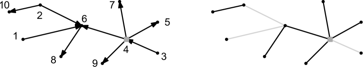
  Figure 3.1: The optimal tree: the numbers on the left are those given by $\widehat{\pi}$. The grey box numbered $4$ is the root. The edges in the right are those retained in the claimed solution.

To prove the claim, root each component of $S^{\star}$ at an arbitrary node, and associate each non-root vertex $u$ with the unique edge $e(u)$ of the undirected graph on the path towards the root. The proposed solution chooses for each vertex $u$, the edge $e(u)=\{u,v\}$ if $\widehat{\pi}(v)<\widehat{\pi}(u)$, i.e., if it is directed into $u$ (Figure 3.1). Since this event happens with probability $1/2$, the proof follows by linearity of expectation.  

This algorithm is order-oblivious because the $50\%$-algorithm has the property. If we don’t care about order-obliviousness, we can instead use the $37\%$-algorithm and get expected value at least $\nicefrac{{V^{\star}}}{{2e}}$.

3.1.3 The Matroid Secretary Problem

One of the most tantalizing generalizations of the secretary problem is to matroids. (A matroid defines a notion of independence for subsets of elements, generalizing linear-independence of a collection of vectors in a vector space. E.g., if we define a subset of edges to be independent if they are acyclic, these form a “graphic” matroid.) Suppose the $n$ items form the ground set elements of a known matroid, and we can pick only subsets of items that are independent in this matroid. The weight/value $V^{\star}$ of the max-weight independent set can be computed offline by the obvious generalization of Kruskal’s greedy algorithm. The open question is to get an expected value of $\Omega(V^{\star})$ online in the RO model. The approach from Theorem 3.2 gives expected value $\Omega(V^{\star}/\log k)$, where $k$ is the largest size of an independent set (its rank). The current best algorithms (which are also order-oblivious) achieve an expected value of $\Omega(V^{\star}/\log\log k)$. Moreover, we can obtain $\Omega(V^{\star})$ for many special classes of matroids by exploiting their special properties, like we did for the graphic matroid above; see the notes for references.

3.2 Order-Adaptive Algorithms

The order-oblivious algorithms above have several benefits, but their competitive ratios are often worse than order-adaptive algorithms where we exploit the randomness of the entire arrival order. Let us revisit the problem of picking $k$ items.

3.2.1 The Multiple-Secretary Problem Revisited

In the order-oblivious case of Section 3.1.1, we ignored the first $\approx k^{-1/3}$ fraction of the items in the first phase, and then chose a fixed threshold to use in the second phase. The length of this initial phase was chosen to balance two competing concerns: we wanted the first phase to be short, so that we ignore few items, but we wanted it to be long enough to get a good estimate of the $k^{th}$ largest item in the entire input. The idea for the improved algorithm is to run in multiple phases and use time-varying thresholds. Roughly, the algorithm uses the first $n_{0}=\delta n$ arrivals to learn a threshold for the next $n_{0}$ arrivals, then it computes a new threshold at time $n_{1}=2n_{0}$ for the next $n_{1}$ arrivals, and so on.

As in the order-oblivious algorithm, we aim for the $(1-\varepsilon)k^{th}$-largest element of $S^{\star}$—that $\varepsilon$ gives us a margin of safety so that we don’t pick a threshold lower than the $k^{th}$-largest (a.k.a. smallest) element of $S^{\star}$. But we vary the value of $\varepsilon$. In the beginning, we have low confidence, so we pick items cautiously (by setting a high $\varepsilon_{0}$ and creating a larger safety margin). As we see more elements, we are more confident in our estimates, and can decrease the $\varepsilon_{j}$ values.

  

1. Set $\delta:=\sqrt{\frac{\log k}{k}}$. Denote $n_{j}:=2^{j}\delta n$ and ignore first $n_{0}=\delta n$ items.

2. For $j\in[0,\log\nicefrac{{1}}{{\delta}}]$, phase $j$ runs on arrivals in window $W_{j}:=(n_{j},n_{j+1}]$

   • Let $k_{j}:=(k/n)n_{j}$ and let $\varepsilon_{j}:=\sqrt{\delta/2^{j}}$.

   • Set threshold $\tau_{j}$ to be the $(1-\varepsilon_{j})k_{j}^{th}$-largest value among the first $n_{j}$ items.

   • Choose any item in window $W_{j}$ with value above $\tau_{j}$ (until budget $k$ is exhausted).

  

Theorem 3.4.

The order-adaptive algorithm above for the multiple-secretary problem has expected value $V^{\star}\big{(}1-O\big{(}\sqrt{\frac{\log k}{k}}\big{)}\big{)}$.

As in Theorem 3.1, we first show that none of the thresholds $\tau_{j}$ are “too low” (so we never run out of budget $k$). Indeed, for $\tau_{j}$ to lie below $v^{\prime}:=\min_{i\in S^{\star}}v_{i}$, less than $(1-\varepsilon_{j})k_{j}$ items from $S^{\star}$ should fall in the first $n_{j}$ items. Since we expect $k_{j}$ of them, the probability of this is at most $\exp(-\varepsilon_{j}^{2}k_{j})=\exp(-\delta^{2}k)=1/\operatorname{poly}(k)$.

Next, we claim that $\tau_{j}$ is not “too high”: it is with high probability at most the value of the $(1-2\varepsilon_{j})k^{th}$ highest item in $S^{\star}$ (thus all thresholds are at most $(1-2\varepsilon_{0})k^{th}$ highest value). Indeed, we expect $(1-2\varepsilon_{j})k_{j}$ of these highest items to appear in the first $n_{j}$ arrivals, and the probability that more than $(1-\varepsilon_{j})k_{j}$ appear is $\exp(-\varepsilon_{j}^{2}k_{j})=1/\operatorname{poly}(k)$.

Taking a union bound over all $j\in[0,\log\nicefrac{{1}}{{\delta}}]$, with high probability all thresholds are neither too high nor too low. Condition on this good event. Now any of the top $(1-2\varepsilon_{0})k$ items will be picked if it arrives after first the $n_{0}$ arrivals (since no threshold is too high and we never run out of budget $k$), i.e., with probability $(1-\delta)$. Similarly, any item which is in top $(1-2\varepsilon_{j+1})k$, but not in top $(1-2\varepsilon_{j})k$, will be picked if it arrives after $n_{j+1}$, i.e., with probability $(1-2^{j+1}\delta)$. Thus if $v_{\max}=v_{1}>\ldots>v_{k}$ are the top $k$ items, we get an expected value of

$$\sum_{i=1}^{(1-2\varepsilon_{0})k}v_{i}(1-\delta)+\sum_{j=0}^{\log\nicefrac{{1}}{{\delta}}-1}~{}\sum_{i=(1-2\varepsilon_{j})k}^{(1-2\varepsilon_{j+1})k}v_{i}(1-2^{j+1}\delta).$$

This is at least $V^{\star}(1-\delta)-\nicefrac{{V^{\star}}}{{k}}\big{(}\sum_{j=0}^{\log\nicefrac{{1}}{{\delta}}}2\varepsilon_{j+1}k\cdot 2^{j+1}\delta\big{)}$ because the negative terms are maximized when the top $k$ items are all equal to $\nicefrac{{V^{\star}}}{{k}}$. Simplifying, we get $V^{\star}(1-O(\delta))$, as claimed.  

The logarithmic term in $\delta$ can be removed (see the notes), but the loss of $\sqrt{k}$ is essential. Here is a sketch of the lower bound. By Yao’s minimax lemma, it suffices to give a distribution over instances that causes a large loss for any deterministic algorithm. Suppose each item has value $0$ with probability $1-\frac{k}{n}$, else it has value $1$ or $2$ with equal probability. The number of non-zero items is therefore $k\pm O(\sqrt{k})$ with high probability, with about half $1$’s and half $2$’s, i.e., $V^{\star}=3k/2\pm O(\sqrt{k})$. Ideally, we want to pick all the $2$’s and then fill the remaining $k/2\pm O(\sqrt{k})$ slots using the $1$’s. However, consider the state of the algorithm after $n/2$ arrivals. Since the algorithm doesn’t know how many $2$’s will arrive in the second half, it doesn’t know how many $1$’s to pick in the first half. Hence, it will either lose about $\Theta(\sqrt{k})$ $2$’s in the second half, or it will pick $\Theta(\sqrt{k})$ too few $1$’s from the first half. Either way, the algorithm will lose $\Omega(V^{\star}/\sqrt{k})$ value.

3.2.2 Solving Packing Integer Programs

The problem of picking a max-value subset of $k$ items can be vastly generalized. Indeed, if each item $i$ has size $a_{i}\in[0,1]$ and we can pick items having total size $k$, we get the knapsack problem. More generally, suppose we have $k$ units each of $d$ different resources, and item $i$ is specified by the amount $a_{ij}\in[0,1]$ of each resource $j\in\{1,\ldots,d\}$ it uses if picked; we can pick any subset of items/vectors which can be supported by our resources. Formally, a set of $n$ different $d$-dimensional vectors $\mathbf{a}_{1},\mathbf{a}_{2},\ldots,\mathbf{a}_{n}\in[0,1]^{d}$ arrive in a random order, each having an associated value $v_{i}$. We can pick any subset of items subject to the associated vectors summing to at most $k$ in each coordinate. (All vectors and values are initially unknown, and on arrival of a vector we must irrevocably pick or discard it.) We want to maximize the expected value of the picked vectors. This gives a packing integer program:

$$\max\sum_{i}v_{i}x_{i}\quad\text{s.t.}\quad\sum_{i}x_{i}\mathbf{a}_{i}\leq k\cdot\mathbf{1}\text{~{}~{}and~{}~{}}x_{i}\in\{0,1\},$$

where the vectors arrive in a random order. Let $V^{\star}:=\max_{\mathbf{x}\in\{0,1\}^{d}}\{\mathbf{v}\cdot\mathbf{x}\mid A\mathbf{x}\leq k\mathbf{1}\}$ be the optimal value, where $A\in[0,1]^{d\times n}$ has columns $\mathbf{a}_{i}$. The multiple-secretary problem is modeled by $A$ having a single row of all ones. By extending the approach from Theorem 3.4 considerably, one can achieve a competitive ratio of $(1-O(\sqrt{(\log d)/k}))$. In fact, several algorithms using varying approaches are known, each giving the above competitive ratio.

We now sketch a weaker result. To begin, we allow the variables to be fractional ($x_{i}\in[0,1]$) instead of integers ($x_{i}\in\{0,1\}$). Since we assume the capacity $k$ is much larger than $\log d$, we can use randomized rounding to go back from fractional to integer solutions with a little loss in value. One of the key ideas is that learning a threshold can be viewed as learning optimal dual values for this linear program.

Theorem 3.5.

There exists an algorithm to solve packing LPs in the RO model to achieve expected value $V^{\star}\big{(}1-O(\sqrt{\frac{d\log n}{k}})\big{)}$.

• (Sketch) The proof is similar to that of Theorem 3.4. The algorithm uses windows of exponentially increasing sizes and (re-)estimates the optimal duals in each window. Let $\delta:=\sqrt{\frac{d\log n}{k}}$; we will motivate this choice soon. As before, let $n_{j}=2^{j}\delta n$, $k_{j}=(k/n)n_{j}$, $\varepsilon_{j}=\sqrt{\delta/2^{j}}$, and the window $W_{j}=(n_{j},n_{j+1}]$. Now, our thresholds are the $d$-dimensional optimal dual variables $\boldsymbol{\tau}_{j}$ for the linear program:

  $$\textstyle{\max\sum_{i=1}^{n_{j}}v_{i}x_{i}\quad\text{s.t.}\quad\sum_{i=1}^{n_{j}}x_{i}\mathbf{a}_{i}\leq(1-\varepsilon_{j})k_{j}\cdot\mathbf{1}\text{~{}~{}and~{}~{}}x_{i}\in[0,1].}$$ (3.1)

  Having computed $\boldsymbol{\tau}_{j}$ at time $n_{j}$, the algorithm picks an item $i\in W_{j}$ if $v_{i}\geq\boldsymbol{\tau}_{j}\cdot\mathbf{a}_{i}$. In the $1$-dimensional multiple-secretary case, the dual is just the value of the $(1-\varepsilon_{j})k_{j}^{th}$ largest-value item among the first $n_{j}$, matching the choice in Theorem 3.4. In general, the dual $\boldsymbol{\tau}_{j}$ can be thought of as the price-per-unit-consumption for every resource; we want to select $i$ only if its value $v_{i}$ is more than the total price $\boldsymbol{\tau}_{j}\cdot\mathbf{a}_{i}$.

  Let us sketch why the dual vector $\boldsymbol{\tau}_{j}$ is not “too low”: i.e., the dual $\boldsymbol{\tau}_{j}$ computed is (with high probability) such that the set $\{\mathbf{a}_{i}\mid\boldsymbol{\tau}_{j}\cdot\mathbf{a}_{i}\leq v_{i},i\in[n]\}$ of all columns that satisfy the threshold $\boldsymbol{\tau}_{j}$ is still feasible. Indeed, suppose a price vector $\boldsymbol{\tau}$ is bad, and using it as threshold on the entire set causes the usage of some resource to exceed $k$. If $\boldsymbol{\tau}$ it is an optimal dual at time $n_{j}$, the usage of that same resource by the first $n_{j}$ items is at most $(1-\varepsilon_{j})k_{j}$ by the LP (3.1). A Chernoff-Hoeffding bound shows that this happens with probability at most $\exp(-\varepsilon_{j}^{2}k_{j})=o(1/n^{d})$, by our choice of $\delta$. Now the crucial idea is to prune the (infinite) set of dual vectors to at most $n^{d}$ by only considering a subset of vectors using which the algorithm makes different decisions. Roughly, there are $n$ choices of prices in each of the $d$ dimensions, giving us $n^{d}$ different possible bad dual vectors; a union-bound now gives the proof.  

As mentioned above, a stronger version of this result has an additive loss $O(\sqrt{\frac{\log d}{k}})V^{\star}$. Such a result is interesting only when $k\gg\log d$, so this is called the “large budget” assumption. How well can we solve packing problems without such an assumption? Specifically, given a downwards-closed family ${\mathcal{F}}\subseteq 2^{[n]}$, suppose we want to pick a subset of items having high total value and lying in ${\mathcal{F}}$. For the information-theoretic question where computation is not a concern, the best known upper bound is $\Omega(V^{\star}/\log^{2}n)$, and there are families where $\Omega(V^{\star}/\frac{\log n}{\log\log n})$ is not possible (see Exercise 2). Can we close this gap? Also, which downward-closed families ${\mathcal{F}}$ admit efficient algorithms with good guarantees?

3.2.3 Max-Weight Matchings

Consider a bipartite graph on $n$ agents and $m$ items. Each agent $i$ has a value $v_{ij}\in\mathbb{R}_{\geq 0}$ for item $j$. The maximum-weight matching problem is to find an assignment $M:[n]\rightarrow[m]$ to maximize $\sum_{i\in[n]}v_{iM(i)}$ such that no item $j$ is assigned to more than one agent, i.e., $|M^{-1}(j)|\leq 1$ for all $j\in[m]$. In the online setting, which has applications to allocating advertisements, the $m$ items are given up-front and the $n$ agents arrive one by one. Upon arriving, agent $i$ reveals their valuations $v_{ij}$ for $j\in[m]$, whereupon we may irrevocably allocate one of the remaining items to $i$. Let $V^{\star}$ denote the value of the optimal matching. The case of $m=1$ with a single item is exactly the single-item secretary problem.

The main algorithmic technique in this section almost seems naïve at first glance: after ignoring the few first arrivals, we make each subsequent decision based on an optimal solution of the arrivals until that point, ignoring all past decisions. For the matching problem, this idea translates to the following:

   Ignore the first $n/e$ agents. When agent $i\in(n/e,n]$ arrives:

1. Compute a max-value matching $M^{(i)}$ for the first $i$ arrivals (ignoring past decisions).

2. If $M^{(i)}$ matches the current agent $i$ to item $j$, and if $j$ is still available, then allocate $j$ to agent $i$; else, give nothing to agent $i$.

  

(We assume that the matching $M^{(i)}$ depends only on the identities of the first $i$ requests, and is independent of their arrival order.) We show the power of this idea by proving that it gives optimal competitiveness for matchings.

Theorem 3.6.

The algorithm gives a matching with expected value at least $V^{\star}/e$.

• There are two insights into the proof. The first is that the matching $M^{(i)}$ is on a random subset of $i$ of the $n$ requests, and so has an expected value at least $(i/n)V^{\star}$. The $i^{th}$ agent is a random one of these and so gets expected value $V^{\star}/n$.

  The second idea is to show, like in Theorem 2.1, that if agent $i$ is matched to item $j$ in $M^{(i)}$, then $j$ is free with probability $\frac{n}{ei}$. Indeed, condition on the set, but not the order, of first $i$ agents (which fixes $M^{(i)}$) and the identity of the $i^{th}$ agent (which fixes $j$). Now for any $k\in(n/e,i)$, the item $j$ was allocated to the $k^{th}$ agent with probability at most $\frac{1}{k}$ (because even if $j$ is matched in $M^{(k)}$, the probability of the corresponding agent being the $k^{th}$ agent is at most $1/k$). The arrival order of the first $k-1$ agents is irrelevant for this event, so we can do this argument for all $s<k$: the probability $j$ was allocated to the $s^{th}$ agent, conditioned on $j$ not being allocated to the $k^{th}$ agent, is at most $\frac{1}{s}$. So the probability that $j$ is available for agent $i$ is at least $\prod_{n/e<k<i}\big{(}1-\frac{1}{k}\big{)}\approx\frac{n}{ei}$. Combining these two ideas and using linearity of expectation, the expected total matching value is at least $\sum_{i=1+n/e}^{n}\big{(}\nicefrac{{n}}{{ei}}\cdot\nicefrac{{V^{\star}}}{{n}}\big{)}\approx\nicefrac{{V^{\star}}}{{e}}.$  

This approach can be extended to combinatorial auctions where each agent $i$ has a submodular (or an XOS) valuation $v_{i}$ and can be assigned a subset $S_{i}\subseteq[m]$ of items; the goal is to maximize total welfare $\sum_{i}v_{i}(S_{i})$. Also, this approach of following the current solution (ignoring past decisions) extends to solving packing LPs: the algorithm solves a slightly scaled-down version of the current LP at each step $i$ and sets the variable $x_{i}$ according to the obtained solution.

4 Minimization Problems

We now study minimization problems in the RO model. In these problems the goal is to minimize some notion of cost (e.g., the length of augmenting paths, or the number of bins) subject to fulfilling some requirements. All the algorithms in this section are order-adaptive. We use $OPT$ to denote both the optimal solution on the instance $S$ and its cost.

4.1 Minimizing Augmentations in Online Matching

We start with one reason why the RO model might help for online discrete minimization problems. Consider a problem to be “well-behaved” if there is always a solution of cost $\approx OPT$ to serve the remaining requests. This is clearly true at the beginning of the input sequence, and we want it to remain true over time—i.e., poor choices in the past should not cause the optimal solution on the remaining requests to become much more expensive. Moreover, suppose that the problem cost is “additive” over the requests. Then satisfying the next request, which by the RO property is a random one of $i$ remaining requests, should cost $\approx OPT/i$ in expectation. Summing over all $n$ requests gives an expected cost of $\approx OPT(\frac{1}{n}+\frac{1}{n-1}+\ldots+\frac{1}{2}+1)=O(\log n)\,OPT$. (This general idea is reminiscent of that for max-weight matchings from §3.2, albeit in a minimization setting.)

To illustrate this idea, we consider an online bipartite matching problem. Let $G=(U,V,E)$ be a bipartite graph with $|U|=|V|=n$. Initially the algorithm does not know the edge set $E$ of the graph, and hence the initial matching $M_{0}=\emptyset$. At each time step $t\in[1,n]$, all edges incident to the $t^{th}$ vertex $u_{t}\in U$ are revealed. If the previous matching $M_{t-1}$ is no longer a maximum matching among the current set of edges, the algorithm must perform an augmentation to obtain a maximum matching $M_{t}$. We do not want the matchings to change too drastically, so we define the cost incurred by the algorithm at step $t$ to be the length of the augmenting path $M_{t-1}\triangle M_{t}$. The goal is to minimize the total cost of the algorithm. (For simplicity, assume $G$ has a perfect matching and $OPT=n$, so we need to augment at each step.) A natural algorithm is shortest augmenting path (see Figure 4.2):

   When a request $u_{t}\in U$ arrives:

1. Augment along a shortest alternating path $P_{t}$ from $u_{t}$ to some unmatched vertex in $V$.

  

Figure 4.2: (i) The graph $G$ with a perfect matching shown by dashed edges. (ii) An intermediate matching $M_{2}$. (iii) The matching $M_{3}$ after the next request arrives at $d$.

Theorem 4.1.

The shortest augmenting path algorithm incurs in total $O(n\log n)$ augmentation cost in expectation in the RO model.

• Fix an optimal matching $M^{*}$, and consider some time step during the algorithm’s execution. Suppose the current maximum matching $M$ has size $n-k$. As a thought experiment, if all the remaining $k$ vertices in $U$ are revealed at once, the symmetric difference $M^{*}\triangle M$ forms $k$ node-disjoint alternating paths from these remaining $k$ vertices to unmatched nodes in $V$. Augmenting along these paths would gives us the optimal matching. The sum of lengths of these paths is at most $|M^{*}|+|M|\leq 2n$. (Observe that the cost of the optimal solution on the remaining requests does increase over time, but only by a constant factor.) Now, since the next vertex is chosen uniformly at random, its augmenting path in the above collection—and hence the shortest augmenting path from this vertex—has expected length at most $2n/k$. Now summing over all $k$ from $n$ down to $1$ gives a total expected cost of $2n\big{(}\frac{1}{n}+\frac{1}{n-1}+\ldots+\frac{1}{2}+1\big{)}=2nH_{n}=O(n\log n)$, hence proving the theorem.  

This $O(\log n)$-competitiveness guarantee happens to be tight for this matching problem in the RO model; see Exercise 3.

4.2 Bin Packing

In the classical bin-packing problem (which you may recall from Chapter 8), the request sequence consists of items of sizes $s_{1},s_{2},\ldots,s_{n}$; these items need to be packed into bins of unit capacity. (We assume each $s_{i}\leq 1$.) The goal is to minimize the number of bins used. One popular algorithm is Best Fit:

   When the next item (with size $s_{t}$) arrives:

1. If the item does not fit in any currently used bin, put it in a new bin. Else,

2. Put into a bin where the resulting empty space is minimized (i.e., where it fits “best”).

  

Best Fit uses no more than $2\,OPT$ bins in the worst case. Indeed, the sum of item sizes in any two of the bins is strictly more than $1$, else we would never have started the later of these bins. Hence we use at most $\lceil 2\sum_{i}s_{i}\rceil$ bins, whereas $OPT$ must be at least $\lceil\sum_{i}s_{i}\rceil$, since each bin holds at most unit total size. A more sophisticated analysis shows that Best Fit uses $1.7\,OPT+O(1)$ bins on any request sequence, and this multiplicative factor of $1.7$ is the best possible.

The examples showing the lower bound of $1.7$ are intricate, but a lower bound of $\nicefrac{{3}}{{2}}$ is much easier to show, and also illustrates why Best Fit does better in the RO model. Consider $n/2$ items of size $\nicefrac{{1}}{{2}}^{-}:=\nicefrac{{1}}{{2}}-\varepsilon$, followed by $n/2$ items of size $\nicefrac{{1}}{{2}}^{+}:=\nicefrac{{1}}{{2}}+\varepsilon$. While the optimal solution uses $n/2$ bins, Best Fit uses $3n/4$ bins on this adversarial sequence, since it pairs up the $\nicefrac{{1}}{{2}}^{-}$ items with each other, and then has to use one bin per $\nicefrac{{1}}{{2}}^{+}$ item. On the other hand, in the RO case, the imbalance between the two kinds of items behaves very similar to a symmetric random walk on the integers. (It is exactly such a random walk, but conditioned on starting and ending at the origin). The number of $\nicefrac{{1}}{{2}}^{+}$ items that occupy a bin by themselves can now be bounded in terms of the maximum deviation from the origin (see Exercise 4), which is $O(\sqrt{n\log n})=o(OPT)$ with high probability. Hence on this instance Best Fit uses only $(1+o(1))\,OPT$ bins in the RO model, compared to $1.5\,OPT$ in the adversarial order. On general instances, we get:

Theorem 4.2.

The Best Fit algorithm uses at most $(1.5+o(1))\,OPT$ bins in the RO setting.

The key insight in the proof of this result is a “scaling” result, saying that any $\varepsilon n$-length subsequence of the input has an optimal value $\varepsilon OPT$, plus lower-order terms. The proof uses the random order property and concentration-of-measure. Observe that the worst-case example does not satisfy this scaling property: the second half of that instance has optimal value $n/2$, the same as for the entire instance. (Such a scaling property is often the crucial difference between the worst-case and RO moels: e.g., we used this in the algorithm for packing LPs in §3.2.2.)

The exact performance of Best Fit in RO model remains unresolved: the best known lower bound uses $1.07\,OPT$ bins. Can we close this gap? Also, can we analyze other common heuristics in this model? E.g., First Fit places the next request in the bin that was started the earliest, and can accommodate the item. Exercise 5 asks you to show that the Next Fit heuristic does not benefit from the random ordering, and has a competitive ratio of $2$ in both the adversarial and RO models.

4.3 Facility Location

A slightly different algorithmic intuition is used for the online facility location problem, which is related to the $k$-means and $k$-median clustering problems. In this problem, we are given a metric space $(V,d)$ with point set $V$, and distances $d:V\times V\to\mathbb{R}_{\geq 0}$ satisfying the triangle inequality. Let $f\geq 0$ be the cost of opening a facility; the algorithm can be extended to cases where different locations have different facility costs. Each request is specified by a point in the metric space, and let $R_{t}=\{r_{1},\ldots,r_{t}\}$ be the (multi)-set of request points that arrive by time $t$. A solution at time $t$ is a set $F_{t}\subseteq V$ of “facilities” whose opening cost is $f\cdot|F_{t}|$, and whose connection cost is the sum of distances from every request to its closest facility in $F_{t}$, i.e., $\sum_{j\in R_{t}}\min_{i\in F_{t}}d(j,i)$. An open facility remains open forever, so we require $F_{t-1}\subseteq F_{t}$. We want the algorithm’s total cost (i.e., the opening plus connection costs) at time $t$ to be at most a constant times the optimal total cost for $R_{t}$ in the RO model. Such a result is impossible in the adversarial arrival model, where a tight $\Theta(\frac{\log n}{\log\log n})$ worst-case competitiveness is known.

There is a tension between the two components of the cost: opening more facilities increases the opening cost, but reduces the connection cost. Also, when request $r_{t}$ arrives, if its distance to its closest facility in $F_{t-1}$ is more than $f$, it is definitely better (in a greedy sense) to open a new facility at $r_{t}$ and pay the opening cost of $f$, than to pay the connection cost more than $f$. This suggests the following algorithm:

   When a request $r_{t}$ arrives:

1. Let $d_{t}:=\min_{i\in F_{t-1}}d(r_{t},i)$ be its distance to the closest facility in $F_{t-1}$.

2. Set $F_{t}\leftarrow F_{t-1}\cup\{r_{t}\}$ with probability $p_{t}:=\min\{1,d_{t}/f\}$, and $F_{t}\leftarrow F_{t-1}$ otherwise.

  

Observe that the choice of $p_{t}$ approximately balances the expected opening cost $p_{t}\cdot f\leq d_{t}$ with the expected connection cost $(1-p_{t})d_{t}\leq d_{t}$. Moreover, since the set of facilities increases over time, a request may be reassigned to a closer facility later in the algorithm; however, the analysis works even assuming the request $r_{t}$ is permanently assigned to its closest facility in $F_{t}$.

Theorem 4.3.

The above algorithm is $O(1)$-competitive in the RO model.

The insight behind the proof is a charging argument that first classifies each request as “easy” (if they are close to a facility in the optimal solution, and hence cheap) or “difficult” (if they are far from their facility). There are an equal number of each type, and the random permutation ensures that easy and difficult requests are roughly interleaved. This way, each difficult request can be paired with its preceding easy one, and this pairing can be used to bound their cost.

5 Related Models and Extensions

There have been other online models related to RO arrival. Broadly, these models can be classified either as “adding more randomness” to the RO model by making further stochastic assumptions on the arrivals, or as “limiting randomness” where the arrival sequence need not be uniformly random. The former lets us exploit the increased stochasticity to design algorithms with better performance guarantees; the latter help us quantify the robustness of the algorithms, and the limitations of the RO model.

5.1 Adding More Randomness

The RO model is at least as general as the i.i.d. model, which assumes a probability distribution $\mathcal{D}$ over potential requests where each request is an independent draw from the distribution $\mathcal{D}$. Hence, all the above RO results immediately translate to the i.i.d. model. Is the converse also true—i.e., can we obtain identical algorithmic results in the two models? The next case study answers this question negatively, and then illustrates how to use the knowledge of the underlying distribution to perform better.

5.1.1 Steiner Tree in the RO model

In the online Steiner tree problem, we are given a metric space $(V,d)$, which can be thought of as a complete graph with edge weights $d(u,v)$; each request is a vertex in $V$. Let $R_{t}=\{r_{1},\ldots,r_{t}\}$ be the (multi)-set of request vertices that arrive by time $t$. When a request $r_{t}$ arrives, the algorithm must pick some edges $E_{t}\subseteq\binom{V}{2}$, so that edges $E_{1}\cup\cdots\cup E_{t}$ picked till now connect $R_{t}$ into a single component. The cost of each edge $\{u,v\}$ is its length $d(u,v)$, and the goal is to minimize the total cost.

The first algorithm we may imagine is the greedy algorithm, which picks a single edge connecting $r_{t}$ to the closest previous request in $R_{t-1}$. This greedy algorithm is $O(\log n)$-competitive for any request sequence of length $n$ in the worst-case. Surprisingly, there are lower bounds of $\Omega(\log n)$, not just for adversarial arrivals, but also for the RO model. Let us discuss how the logarithmic lower bound for the adversarial model translates to one for the RO model.

There are two properties of the Steiner tree problem that make this transformation possible. The first is that duplicating requests does not change the cost of the Steiner tree, but making many copies of a request makes it likely that one of these copies will appear early in the RO sequence. Hence, if we take a fixed request sequence $\sigma$, duplicate the $i^{th}$ request $C^{n-i}$ times (for some large $C>1$), apply a uniform random permutation, and remove all but the first copy of each original request, the result looks close to $\sigma$ with high probability. Of course, the sequence length increases from $n$ to $\approx C^{n}$, and hence the lower bound goes from being logarithmic to being doubly logarithmic in the sequence length.

We now use a second property of Steiner tree: the worst-case examples consist of $n$ requests that can be given in $\log n$ batches, with the $i^{th}$ batch containing $\approx 2^{i}$ requests—it turns out that giving so much information in parallel does not help the algorithm. Since we don’t care about the relative ordering within the batches, we can duplicate the requests in the $i^{th}$ batch $C^{i}$ times, thereby making the resulting request sequences of length $\leq C^{1+\log n}$. It is now easy to set $C=n$ to get a lower bound of $\Omega(\frac{\log n}{\log\log n})$, but a careful analysis allows us to set $C$ to be a constant, and get an $\Omega(\log n)$ lower bound for the RO setting.

5.1.2 Steiner Tree in the i.i.d. model

Given this lower bound for the RO model, what if we make stronger assumptions about the randomness in the input? What if the arrivals are i.i.d. draws from a probability distribution? We now have to make an important distinction, whether the distribution is known to the algorithm or not. The lower bound of the previous section can easily be extended to the case where arrivals are from an unknown distribution, so our only hope for a positive result is to consider the i.i.d. model with known distributions. In other words, each request is a random vertex of the graph, where vertex $v$ is requested with a known probability $p_{v}\geq 0$ (and $\sum_{v}p_{v}=1$). Let $\mathbf{p}=(p_{1},p_{2},\ldots,p_{|V|})$ be the vector of these probabilities. For simplicity, assume that we know the length $n$ of the request sequence. The augmented greedy algorithm is the following:

  

1. Let $A$ be the (multi-)set of $n-1$ i.i.d. samples from the distribution $\bf{p}$, plus the first request $r_{1}$.

2. Build a minimum spanning tree $T$ connecting all the vertices in $A$.

3. For each subsequent request $r_{i}$ (for $i\geq 2$): connect $r_{i}$ to the closest vertex in $A\cup R_{i-1}$ using a direct edge.

  

Note that our algorithm requires minimal knowledge of the underlying distribution: it merely takes a set of samples that are stochastically identical to the actual request sequence, and builds the “anticipatory” tree connecting this sample. Now the hope is that the real requests will look similar to the samples, and hence will have close-by vertices to which they can connect.

Theorem 5.1.

The augmented greedy algorithm is $4$-competitive for the Steiner tree problem in the setting of i.i.d. requests with known distributions.

• Since set $A$ is drawn from the same distribution as the actual request sequence $R_{n}$, the expected optimal Steiner tree on $A$ also costs $OPT$. The minimum spanning tree to connect up $A$ is known to give a $2$-approximate Steiner tree (Exercise 6), so the expected cost for $T$ is $2OPT$.

  Next, we need to bound the expected cost of connecting $r_{t}$ to the previous tree for $t\geq 2$. Let the samples in $A$ be called $a_{2},a_{3},\ldots,a_{n}$. Root the tree $T$ at $r_{1}$, and let the “share” of $a_{t}$ from $T$ be the cost of the first edge on the path from $a_{t}$ to the root. The sum of shares equals the cost of $T$. Now, the cost to connect $r_{t}$ is at most the expected minimum distance from $r_{t}$ to a vertex in $A\setminus\{a_{t}\}$. But $r_{t}$ and $a_{t}$ are from the same distribution, so this expected minimum distance is bounded by the expected distance from $a_{t}$ to its closest neighbor in $T$, which is at most the expected share of $a_{t}$. Summing, the connection costs for the $r_{t}$ requests is at most the expected cost of $T$, i.e., at most $2OPT$. This completes the proof.  

The proof above extends to the setting where different requests are drawn from different known distributions; see Exercise 6.

5.2 Reducing the Randomness

Do we need the order of items to be uniformly random, or can weaker assumptions suffice for the problems we care about? This question was partially addressed in §3.1 where we saw order-oblivious algorithms. Recall: these algorithms assume a less-demanding arrival model, where a random fraction of the adversarial input set $S$ is revealed to the algorithm in a first phase, and the remaining input set arrives in an adversarial order in the second phase. We now discuss some other models that have been proposed to reduce the amount of randomness required from the input. While some remarkable results have been obtained in these directions, there is still much to explore.

5.2.1 Entropy of the random arrival order

One principled way of quantifying the randomness is to measure the entropy of the input sequences: a uniformly random permutation on $n$ items has entropy $\log(n!)=O(n\log n)$, whereas order-oblivious algorithms (where each item is put randomly in either phase) require at most $\log{{n}\choose{n/2}}\leq n$ bits of entropy. Are there arrival order distributions with even less entropy for which we can give good algorithms?

This line of research was initiated by Kesselheim et al., (2015), who showed the existence of arrival-order distributions with entropy only $O(\log\log n)$ that allow $e$-competitive algorithms for the single-item secretary problem (and also for some simple multiple-item problems). Moreover, they showed tightness of their results—for any arrival distribution with $o(\log\log n)$ entropy no online algorithm can be $O(1)$-competitive. This work also defines a notion of “almost $k$-wise uniformity”, which requires that the induced distribution on every subset of $k$ items be close to uniform. They show that this property and its variants suffice for some of the algorithms, but not for all.

A different perspective is the following: since the performance analysis for an algorithm in the RO model depends only on certain randomness properties of the input sequence (which are implied by the random ordering), it may be meaningful in some cases to (empirically) verify these specific properties on the actual input stream. E.g., Bahmani et al., (2010) used this approach to explain the experimental efficacy of their algorithm computing personalized pageranks in the RO model.

5.2.2 Robustness and the RO Model

The RO model assumes that the adversary first chooses all the item values, and then the arrival order is perturbed at random according to some specified process. While this is a very appealing framework, one concern is that the algorithms may over-fit the model. What if, as in some other semi-random models, the adversary gets to make a small number of changes after the randomness has been added? Alternatively, what if some parts of the input must remain in adversarial order, and the remainder is randomly permuted? For instance, say the adversary is allowed to specify a single item which must arrive at some specific position in the input sequence, or it is allowed to change the position of a single item after the randomness has been added. Most current algorithms fail when faced with such modest changes to the model. E.g., the 37%-algorithm picks nothing if the adversary presents a large item in the beginning. Of course, these algorithms were not designed to be robust: but can we get analogous results even if the input sequence is slightly corrupted?

One approach is to give “best-of-both-worlds” algorithms that achieve a good performance when the input is randomly permuted, and which also have a good worst-case performance in all cases. For instance, Mirrokni et al., (2012) and Raghvendra, (2016) give such results for online ad allocation and min-cost matching, respectively. Since the secretary problem has poor performance in the worst case, we may want more refined guarantees, that the performance degrades with the amount of corruption. Here is a different semi-random model for the multiple-secretary problem from §3.1.1. In the Byzantine model, the adversary not only chooses the values of all $n$ items, it also chooses the relative or absolute order of some $\varepsilon n$ of these items. The remaining $(1-\varepsilon)n$ “good” items are then randomly permuted within the remaining positions. The goal is now to compare to the top $k$ items among only these good items. Some preliminary results are known for this model (Bradac et al.,, 2020), but many questions remain open. In general, getting robust algorithms for secretary problems, or other optimization problems considered in this chapter, remains an important direction to explore.

5.3 Extending Random-Order Algorithms to Other Models

Algorithms for the RO model can help in designing good algorithms for similar models. One such example is for the prophet model, which is closely related to the optimal stopping problem in §1.1.4 of Chapter 8. In this model, we are given $n$ independent prize-value distributions $D_{1},\ldots,D_{n}$, and then presented with draws $v_{i}\sim D_{i}$ from these distributions in adversarial order. The threshold rule from Chapter 8, which picks the first prize with value above some threshold computable from just the distributions, gets expected value at least $\frac{1}{2}{\mathbb{E}}[\max_{i}v_{i}]$. Note the differences between the prophet and RO models: the prophet model assumes more about the values—namely, that they are drawn from the given distributions—but less about the ordering, since the items can be presented in an adversarial order. Interestingly, order-oblivious algorithms in the RO model can be used to get algorithms in the prophet model.

Indeed, suppose we only have limited access to the distributions $D_{i}$ in the prophet model: we can only get information about them by drawing a few samples from each distribution. (Clearly we need at least one sample from the distributions, else we would be back in the online adversarial model.) Can we use these samples to get algorithms in this limited-access prophet model for some packing constraint family ${\mathcal{F}}$? The next theorem shows we can convert order-oblivious algorithms for the RO model to this setting using only a single sample from each distribution.

Theorem 5.2.

Given an $\alpha$-competitive order-oblivious online algorithm for a packing problem ${\mathcal{F}}$, there exists an $\alpha$-competitive algorithm for the corresponding prophet model with unknown probability distributions, assuming we have access to one (independent) sample from each distribution.

The idea is to choose a random subset of items to be presented to the order-oblivious algorithm in the first phase; for these items we send in the sampled values available to us, and for the remaining items we use their values among the actual arrivals. The details are left as Exercise 7.

6 Notes

The classical secretary problem and its variants have long been studied in optimal stopping theory; see Ferguson, (1989) for a historical survey. In computer science, the RO model has been used, e.g., for computational geometry problems, to get fast and elegant algorithms for problems like convex hulls and linear programming; see Seidel, (1993) for a survey in the context of the backwards analysis technique. The secretary problem has gained broader attention due to connections to strategyproof mechanism design for online auctions (Hajiaghayi et al.,, 2004; Kleinberg,, 2005). Theorem 2.2 is due to Gilbert and Mosteller, (1966).

§3.1: The notion of an order-oblivious algorithm was first defined by Azar et al., (2014). The order-oblivious multiple-secretary algorithm is folklore. The matroid secretary problem was proposed by Babaioff et al., (2018); Theorem 3.2 is an adaptation of their $O(\log r)$-competitive algorithm for general matroids. Theorem 3.3, due to Korula and Pál, (2009), extends to a ${2e}$-competitive order-adaptive algorithm. The current best algorithm is $4$-competitive (Soto et al.,, 2018). The only lower bound known is the factor of $e$ from Theorems 2.1 and 2.2, even for arbitrary matroids, whereas the best algorithm for general matroids has competitive ratio $O(\log\log\text{rank})$ (Lachish,, 2014; Feldman et al.,, 2015). See the survey by Dinitz, (2013) for work leading up to these results.

§3.2: The order-adaptive algorithms for multiple-secretary (Theorem 3.4) and for packing LPs (Theorem 3.5) are based on the work of Agrawal et al., (2014). The former result can be improved to give $(1-O(\sqrt{\nicefrac{{1}}{{k}}}))$-competitiveness (Kleinberg,, 2005). Extending work on the AdWords problem (see the monograph by Mehta, (2012)), Devanur and Hayes, (2009) studied packing LPs in the RO model. The optimal results have $(1-O(\sqrt{(\log d_{\text{nnz}})/k}))$-competitiveness (Kesselheim et al.,, 2014), where $d_{\text{nnz}}$ is the maximum number of non-zeros in any column; these are based on the solve-ignoring-past-decisions approach we used for max-value matchings. Rubinstein, (2016) and Rubinstein and Singla, (2017) gave $O(\operatorname{poly}\log n)$-competitive algorithms for general packing problems for subadditive functions. Theorem 3.6 (and extensions to combinatorial auctions) is due to Kesselheim et al., (2013).

§4: Theorem 4.1 about shortest augmenting paths is due to Chaudhuri et al., (2009). A worst-case result of $O(\log^{2}n)$ was given by Bernstein et al., (2018); closing this gap remains an open problem. The analysis of Best Fit in Theorem 4.2 is by Kenyon, (1996). Theorem 4.3 for facility location is by Meyerson, (2001); see Meyerson et al., (2001) for other network design problems in the RO setting. The tight nearly-logarithmic competitiveness for adversarial arrivals is due to Fotakis, (2008).

§5.1: Theorem 5.1 for Steiner tree is by Garg et al., (2008). Grandoni et al., (2013) and Dehghani et al., (2017) give algorithms for set cover and $k$-server in the i.i.d. or prophet models. The gap between the RO and i.i.d. models (with unknown distributions) remains an interesting direction to explore. Correa et al., (2019) show that the single-item problem has the same competitiveness in both models; can we show similar results (or gaps) for other problems?

§5.2: Kesselheim et al., (2015) study connections between entropy and the RO model. The RO model with corruptions was proposed by Bradac et al., (2020), who also give $(1-\varepsilon)$-competitive algorithms for the multiple-secretary problem with weak estimates on the optimal value. A similar model for online matching for mixed (stochastic and worst-case) arrivals was studied by Esfandiari et al., (2015). Finally, Theorem 5.2 to design prophet inequalities from samples is by Azar et al., (2014). Connections between the RO model and prophet inequalities have also been studied via the prophet secretary model where both the value distributions are given and the arrivals are in a uniformly random-order (Esfandiari et al.,, 2017; Ehsani et al.,, 2018).

Acknowledgments

We thank Tim Roughgarden, C. Seshadhri, Matt Weinberg, and Uri Feige for their comments on an initial draft of this chapter.

Exercises

1. Show that both algorithms proposed above Theorem 3.1 for the multiple secretary problem achieve expected value $\Omega(V^{\star})$.

2. Show why for a general packing constraint family ${\mathcal{F}}$, i.e. $A\in{\mathcal{F}}$ and $B\subseteq A$ implies $B\in{\mathcal{F}}$, no online algorithm has $o(\frac{\log n}{\log\log n})$-competitiveness. [Hint: Imagine $n$ elements in a $\sqrt{n}\times\sqrt{n}$ matrix and ${\mathcal{F}}$ consists of subsets of columns.]

3. Consider a cycle on $2n$ vertices, and hence it has a perfect matching. Show that the shortest augmenting path algorithm for minimizing augmentations in online matching from §4.1 has $\Omega(n\log n)$ cost in expectation.

4. Suppose $n/2$ items of size $\nicefrac{{1}}{{2}}^{-}:=\nicefrac{{1}}{{2}}-\varepsilon$ and $n/2$ items of size $\nicefrac{{1}}{{2}}^{+}:=\nicefrac{{1}}{{2}}+\varepsilon$ are presented in a random order to the Best Fit bin packing heuristic from §4.2. Define the imbalance $I_{t}$ after $t$ items to be the number of $\nicefrac{{1}}{{2}}^{+}$ items minus the number of $\nicefrac{{1}}{{2}}^{-}$ items. Show that the number of bins which have only a single item (and hence waste about $\nicefrac{{1}}{{2}}$ space) is at most $(\max_{t}I_{t})-(\min_{t}I_{t})$. Use a Chernoff-Hoeffding bound to prove this is at most $O(\sqrt{n\log n})$ with probability $1-1/\operatorname{poly}(n)$.

5. In the Next Fit heuristic for the bin packing problem from §4.2, the next item is added to the current bin if it can accommodate the item, otherwise we put the item into a new bin. Show that this algorithm has a competitive ratio of $2$ in both the adversarial and RO models.

6. Show that for a set of requests in a metric space, the minimum spanning tree on this subset gives a $2$-approximate solution to the Steiner tree. Also, extend the Steiner tree algorithm from the i.i.d. model to the prophet model, where the $n$ requests are drawn from $n$ independent (possibly different) known distributions $\mathbf{p}^{t}$ over the vertices.

7. Prove Theorem 5.2.

8. Suppose the input consists of $(1-\varepsilon)n$ good items and $\varepsilon n$ bad items. The adversary decides all $n$ item values, and also the locations of bad items. The good items are then randomly permuted in the remaining positions. If $v^{*}$ denotes the value of the largest good item, show there is no online algorithm with expected value $\Omega(v^{*}/(\varepsilon n))$. [Hint: There is only one non-zero good item and all the bad items have values much smaller than $v^{*}$. The bad items are arranged as the single-item adversarial arrival lower bound instance.]

References

- Agrawal et al., (2014) Agrawal, Shipra, Wang, Zizhuo, and Ye, Yinyu. 2014. A Dynamic Near-Optimal Algorithm for Online Linear Programming. Operations Research, 62(4).
- Azar et al., (2014) Azar, Pablo D., Kleinberg, Robert, and Weinberg, S. Matthew. 2014. Prophet inequalities with limited information. In: SODA. ACM, New York.
- Babaioff et al., (2018) Babaioff, Moshe, Immorlica, Nicole, Kempe, David, and Kleinberg, Robert. 2018. Matroid Secretary Problems. J. ACM, 65(6), 35:1–35:26.
- Bahmani et al., (2010) Bahmani, Bahman, Chowdhury, Abdur, and Goel, Ashish. 2010. Fast Incremental and Personalized PageRank. PVLDB, 4(3), 173–184.
- Bernstein et al., (2018) Bernstein, Aaron, Holm, Jacob, and Rotenberg, Eva. 2018. Online Bipartite Matching with Amortized Replacements. Pages 947–959 of: SODA.
- Bradac et al., (2020) Bradac, Domagoj, Gupta, Anupam, Singla, Sahil, and Zuzic, Goran. 2020. Robust Algorithms for the Secretary Problem. Pages 32:1–32:26 of: ITCS.
- Chaudhuri et al., (2009) Chaudhuri, Kamalika, Daskalakis, Constantinos, Kleinberg, Robert D., and Lin, Henry. 2009. Online Bipartite Perfect Matching With Augmentations. Pages 1044–1052 of: INFOCOM.
- Correa et al., (2019) Correa, José R., Dütting, Paul, Fischer, Felix A., and Schewior, Kevin. 2019. Prophet Inequalities for I.I.D. Random Variables from an Unknown Distribution. Pages 3–17 of: EC.
- Dehghani et al., (2017) Dehghani, Sina, Ehsani, Soheil, Hajiaghayi, MohammadTaghi, Liaghat, Vahid, and Seddighin, Saeed. 2017. Stochastic k-Server: How Should Uber Work? Pages 126:1–126:14 of: ICALP.
- Devanur and Hayes, (2009) Devanur, Nikhil R., and Hayes, Thomas P. 2009. The adwords problem: online keyword matching with budgeted bidders under random permutations. Pages 71–78 of: EC.
- Dinitz, (2013) Dinitz, Michael. 2013. Recent advances on the matroid secretary problem. SIGACT News, 44(2), 126–142.
- Ehsani et al., (2018) Ehsani, Soheil, Hajiaghayi, MohammadTaghi, Kesselheim, Thomas, and Singla, Sahil. 2018. Prophet Secretary for Combinatorial Auctions and Matroids. Pages 700–714 of: SODA.
- Esfandiari et al., (2015) Esfandiari, Hossein, Korula, Nitish, and Mirrokni, Vahab S. 2015. Online Allocation with Traffic Spikes: Mixing Adversarial and Stochastic Models. In: EC.
- Esfandiari et al., (2017) Esfandiari, Hossein, Hajiaghayi, MohammadTaghi, Liaghat, Vahid, and Monemizadeh, Morteza. 2017. Prophet secretary. SIAM Journal on Discrete Mathematics, 31(3), 1685–1701.
- Feldman et al., (2015) Feldman, Moran, Svensson, Ola, and Zenklusen, Rico. 2015. A Simple O(log log(rank))-Competitive Algorithm for the Matroid Secretary Problem. Pages 1189–1201 of: SODA.
- Ferguson, (1989) Ferguson, Thomas S. 1989. Who solved the secretary problem? Statistical science, 4(3), 282–289.
- Fotakis, (2008) Fotakis, Dimitris. 2008. On the Competitive Ratio for Online Facility Location. Algorithmica, 50(1), 1–57.
- Garg et al., (2008) Garg, Naveen, Gupta, Anupam, Leonardi, Stefano, and Sankowski, Piotr. 2008. Stochastic analyses for online combinatorial optimization problems. In: SODA.
- Gilbert and Mosteller, (1966) Gilbert, John P., and Mosteller, Frederick. 1966. Recognizing the Maximum of a Sequence. Journal of the American Statistical Association, 61(313), 35–73.
- Grandoni et al., (2013) Grandoni, Fabrizio, Gupta, Anupam, Leonardi, Stefano, Miettinen, Pauli, Sankowski, Piotr, and Singh, Mohit. 2013. Set Covering with Our Eyes Closed. SIAM J. Comput., 42(3), 808–830.
- Hajiaghayi et al., (2004) Hajiaghayi, Mohammad Taghi, Kleinberg, Robert D., and Parkes, David C. 2004. Adaptive limited-supply online auctions. Pages 71–80 of: EC.
- Kenyon, (1996) Kenyon, Claire. 1996. Best-fit bin-packing with random order. In: SODA.
- Kesselheim et al., (2013) Kesselheim, Thomas, Radke, Klaus, Tönnis, Andreas, and Vöcking, Berthold. 2013. An Optimal Online Algorithm for Weighted Bipartite Matching and Extensions to Combinatorial Auctions. Pages 589–600 of: ESA.
- Kesselheim et al., (2014) Kesselheim, Thomas, Radke, Klaus, Tönnis, Andreas, and Vöcking, Berthold. 2014. Primal beats dual on online packing LPs in the random-order model. In: STOC.
- Kesselheim et al., (2015) Kesselheim, Thomas, Kleinberg, Robert D., and Niazadeh, Rad. 2015. Secretary Problems with Non-Uniform Arrival Order. Pages 879–888 of: STOC.
- Kleinberg, (2005) Kleinberg, Robert. 2005. A multiple-choice secretary algorithm with applications to online auctions. In: SODA.
- Korula and Pál, (2009) Korula, Nitish, and Pál, Martin. 2009. Algorithms for Secretary Problems on Graphs and Hypergraphs. Pages 508–520 of: ICALP.
- Lachish, (2014) Lachish, Oded. 2014. O(log log Rank) Competitive Ratio for the Matroid Secretary Problem. Pages 326–335 of: FOCS.
- Mehta, (2012) Mehta, Aranyak. 2012. Online matching and ad allocation. Found. Trends Theor. Comput. Sci., 8(4), 265–368.
- Meyerson, (2001) Meyerson, Adam. 2001. Online Facility Location. Pages 426–431 of: FOCS.
- Meyerson et al., (2001) Meyerson, Adam, Munagala, Kamesh, and Plotkin, Serge A. 2001. Designing Networks Incrementally. Pages 406–415 of: FOCS.
- Mirrokni et al., (2012) Mirrokni, Vahab S., Gharan, Shayan Oveis, and Zadimoghaddam, Morteza. 2012. Simultaneous approximations for adversarial and stochastic online budgeted allocation. Pages 1690–1701 of: SODA.
- Raghvendra, (2016) Raghvendra, Sharath. 2016. A robust and optimal online algorithm for minimum metric bipartite matching. Pages Art. No. 18, 16 of: APPROX-RANDOM. Leibniz Int. Proc. Inform., vol. 60.
- Rubinstein, (2016) Rubinstein, Aviad. 2016. Beyond matroids: secretary problem and prophet inequality with general constraints. Pages 324–332 of: STOC.
- Rubinstein and Singla, (2017) Rubinstein, Aviad, and Singla, Sahil. 2017. Combinatorial prophet inequalities. Pages 1671–1687 of: SODA.
- Seidel, (1993) Seidel, Raimund. 1993. Backwards analysis of randomized geometric algorithms. Pages 37–67 of: New trends in discrete and computational geometry. Algorithms Combin., vol. 10. Springer, Berlin.
- Soto et al., (2018) Soto, José A., Turkieltaub, Abner, and Verdugo, Victor. 2018. Strong Algorithms for the Ordinal Matroid Secretary Problem. Pages 715–734 of: SODA.