Spatially resolved spectroscopy of close massive visual binaries with HST/STIS: I. Seven O-type systems.

Abstract

Context. Many O-type stars have nearby companions whose presence hamper their characterization through spectroscopy.

Aims. We want to obtain spatially resolved spectroscopy of close O-type visual binaries to derive their spectral types.

Methods. We use the Space Telescope Imaging Spectrograph (STIS) of the Hubble Space Telescope (HST) to obtain long-slit blue-violet spectroscopy of eight Galactic O-type stars with nearby visual companions and use spatial-profile fitting to extract the separate spectra. We also use the ground-based Galactic O-Star Spectroscopic Survey (GOSSS) to study more distant visual components.

Results. We spatially resolve seven of the eight systems, present spectra for their components, and obtain their spectral types. Those seven multiple systems are $\iota$ Ori Aa,Ab,B, 15 Mon Aa,Ab,C, $\tau$ CMa Aa,Ab,B,C,D,E, HD 206 267 Aa,Ab,C,D, HD 193 443 A,B, HD 16 429 Aa,Ab, and IU Aur A,B. This is the first time that spatially resolved spectroscopy of the close visual binaries of those systems is obtained. We establish the applicability of the technique as a function of the separation and magnitude difference of the binary.

1 Introduction

 For many years now we have been studying the multiplicity of O stars using different spectroscopic, imaging, and interferometric techniques. Such a combination is needed because even though most (if not all) massive stars are born in multiple systems, the different periods, inclinations, mass ratios, distances, and extinctions make each detection technique more adequate for one or another of the hundreds of O-type multiple systems known. One preliminary aspect of the study of such systems is their identification as O stars, something we are doing with the Galactic O-Star Spectroscopic Survey (GOSSS, Maíz Apellániz et al. 2011). The subsequent cataloguing and spectroscopic characterization of multiple O-type systems is being done with the MONOS project in the northern hemisphere (Maíz Apellániz et al. 2019, from now on MONOS-I) and with the OWN project in the southern hemisphere (Barbá et al., 2010, 2017).

Massive multiple systems with small plane-of-the sky separations $d$ are typically studied using multi-epoch high-resolution spectroscopy, as most such systems known in the Galaxy have short periods ($\lesssim$1 a) that yield significant differences in velocity between the two components that allow spectroscopic orbits to be calculated (possibly with the help of eclipses for the shortest periods with high orbital inclinations). Multiple systems with $d$ of a few arcseconds or more can be easily resolved from the ground and spectra for the different components thus obtained. This leaves a problematic $d$ range between $\approx$30 mas and $\approx$3″, where velocity differences are usually small and the spectra cannot be easily separated from the ground. Furthermore, a large fraction of the O-type multiple systems are not binaries but triples, quadruples, or worse (Sota et al., 2014; Maíz Apellániz et al., 2019) and in those cases where three or more massive stars are located within 3″, the identification of which star corresponds to which spectral type can become a difficult task.

To tackle that problematic range, three years ago we developed the new lucky spectroscopy technique (Maíz Apellániz et al., 2018), which is the spectroscopic equivalent to lucky imaging (Law et al., 2006; Baldwin et al., 2008; Smith et al., 2009). With lucky spectroscopy one obtains a large number of short spectroscopic exposures, selects the ones with better seeing qualities, combines the result, and extracts the resulting spectra fitting a double or triple profile. In Maíz Apellániz et al. (2018) we used the ISIS spectrograph at the William Herschel Telescope (WHT) at La Palma to spatially separate five close visual systems with massive stars and in subsequent observations we have been successful with several tens more (Maíz Apellániz et al. in preparation). However, in the process it has also become clear that lucky spectroscopy has its limitations and that (at least in the configuration we are using) it cannot resolve systems in the lower part of the 30 mas-3″ interval. If we want to obtain spatially separated spectra in the lower part of that range we need to resort to the Hubble Space Telescope (HST) and that is what we have done in this paper. In the next section we describe our data and methods, in section 3 we present our results, and in the last section we analyze them and discuss our future work.

Table 1: HST/STIS sample in this paper plus a system previously observed with this technique (HD 93 129 Aa,Ab). The position angle $\theta$ corresponds to the angle of the slit as measured from the first to the second component while $d^{\prime}$ corresponds to the plane-of-the-sky separation between the two components along the slit. An asterisk is added for those cases where $\Delta B$ or $d^{\prime}$ were fixed from the literature instead of measured from the data. The separation marked with a $\dagger$ was measured with the slit positioned far from the predicted position angle, making $d$ and $d^{\prime}$ significantly different (see text). Measured uncertainties are typically 0.01 mag in $\Delta B$ and 1 mas in $d^{\prime}$.

name	$\Delta B$	$d^{\prime}$	$\theta$	WDS ID	obs. date	res.?
	(mag)	(mas)	(deg)		(YYMMDD)
$\zeta$ Ori Aa,Ab	2.20*	39*	280	05407$-$0157	191118	N
$\iota$ Ori Aa,Ab	3.16	155*	98	05354$-$0555	191119	Y
15 Mon Aa,Ab	1.55	143	269	06410$+$0954	191129	Y
$\tau$ CMa Aa,Ab	0.90	95	310	07187$-$2457	200102	Y
$\tau$ CMa Aa,E	4.47	685$\dagger$	310	07187$-$2457	200102	Y
HD 206 267 Aa,Ab	0.95	64	147	21390$+$5729	191206	Y
HD 193 443 A,B	0.26	138	250	20189$+$3817	191013	Y
HD 16 429 Aa,Ab	2.02	275	91	02407$+$6117	191126	Y
IU Aur A,B	2.04	138*	232	05279$+$3447	191003	Y
HD 93 129 Aa,Ab	1.23	36*	14	10440$-$5933	100407	Y

2 Methods and data

2.1 Sample selection

 To select our sample we used the Galactic O-Star Catalog (GOSC, Maíz Apellániz et al. 2004; Maíz Apellániz et al. 2017a) and searched for bright Galactic O-type close visual systems of astrophysical interest. More specifically, we searched for systems located in the separation-$B$ magnitude difference ($d-\Delta B$) plane not accessible to being spatially resolved using current lucky spectroscopy capabilities (Maíz Apellániz et al., 2018) but that could be resolved in the blue-violet region using HST/STIS based on our previous past experience (Maíz Apellániz et al., 2017b). Our full sample has ten such systems and is being observed with HST GO program 15 815. One of the systems ($\theta^{1}$ Ori Ca,Cb) has not been observed as of the time of this writing and the visit for another one (HD 193 322 Aa,Ab) failed to acquire data correctly and will have to be repeated. Therefore, the sample for this paper includes only eight systems; the other two will be analyzed in future papers. The systems are listed in Table 1 where, for completeness, we have added another system (HD 93 129 Aa,Ab) previously observed by us using the same technique with data from HST GO program 11 784.

2.2 Data acquisition and processing

 We used the same observing technique applied to the HD 93 129 Aa,Ab case mentioned above (Maíz Apellániz et al., 2017b). We obtain STIS exposures with five G430M settings that yield a continuous coverage of the 3793-5104 Å range. To increase the effective spatial resolution a two-point dithering pattern along the slit is applied so that for each grating setting we end up with a 1024$\times$2048 (spectral $\times$ spatial) pixel array. The wavelength coverage is determined by the number of grating settings that can be fit in an orbit (five), as our targets are bright and require only short exposures and most of the time in the orbit is actually consumed by overheads.

The position angle of the slit $\theta$ was chosen to be as close as the telescope scheduling allowed to the expected position angle between the two components (with a possible 180^o offset). We were able to achieve the desired value within 1^o in all cases except in two: $\zeta$ Ori Aa,Ab, where the difference was 4^o and $\iota$ Ori Aa,Ab, where the difference was 6^o. Note that the cosines of those angles are larger than 0.99 so the difference between $d$ and its projection along the slit $d^{\prime}$ should be small. For $\tau$ CMa we unintentionally also recorded a third component in the slit (E). In that case, the Aa,E position angle is expected to be 267^o (there is a 180^o offset in some of the previously published data, see below), so there is a difference of 43^o with $\theta$. We use the 52X2 slit ($52\arcsec\times 2\arcsec$ or $1024\times 39$ STIS/CCD pixels), so the expected 940 mas separation between Aa and E translates into 687 mas along the slit ($y$ in the detector) and 641 mas in the direction perpendicular to it ($x$ in the detector), which corresponds well to the measured values (see below). That may translate into a small slit loss not accounted for in our $\Delta B$ and into an artificial velocity shift for E (which we indeed detect).

 

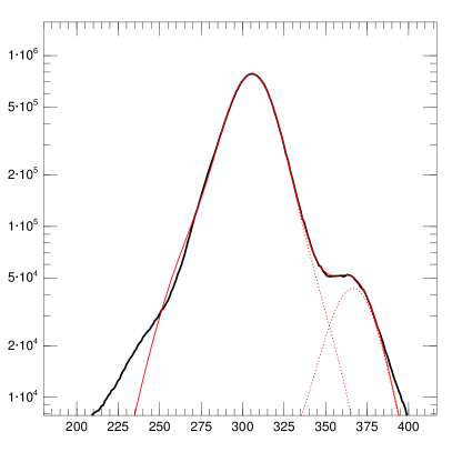
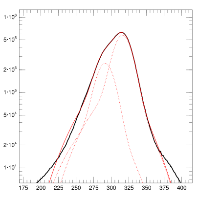
Figure 1: Spatially dithered spectral data collapsed along the trace used to fit the double spatial profile for two of the systems in this paper ($\iota$ Ori Aa,Ab, left, and HD 206 267 Aa,Ab, right, in both cases for the 3936 grating setting). The horizontal axes show the 20x dithered spatial pixels (1 dithered pixel = 2.5 mas) and the vertical axes the counts (in log scale). In each plot the black line is the data, the solid red line the double (Aa+Ab) profile, and the dotted red lines the individual (Aa and Ab) profiles. The left plot is an example with relatively large separation and $\Delta B$ while the right one is an example of the opposite circumstances. See Fig. 1 of Maíz Apellániz et al. (2018) for equivalent plots using lucky spectroscopy.

The spectra were extracted using the techniques derived for MULTISPEC (Maíz Apellániz, 2005a), which were based in part on the theoretical fundaments presented by Porter et al. (2004) and that were further developed for the analysis of the STIS HD 93 129 Aa,Ab data in Maíz Apellániz et al. (2017b) and for lucky spectroscopy in Maíz Apellániz et al. (2018). In the STIS CCD spectra the trace is nearly aligned with the $x$ axis of the detector but not exactly so. To determine the spatial profile that will be used to separate the two components in each system, we first calculated the centroid in the $y$ direction at each of the 1024 $x$ positions of the 1024$\times$2048 pixel array for each grating setting independently. The resulting $y_{c}(x)$ was fitted with a third- or (if needed) a fourth-degree polynomial to determine the trace. As there is a large number of photons collected in each exposure we can accurately determine a dithered spatial profile (Fruchter & Hook, 2002) and fit a functional form to it in the following manner:

• We multiply $y_{c}(x)$ by ten, round off the result, and classify each $x$ position by its last digit (from 0 to 9), a value we will call $R$. This determines how is the trace centered with respect to a pixel center at each value of $x$. Following the convention where a pixel center has an integer coordinate value and an edge a half-integer one, if $R(x)$ is 0 then the trace there is centered at the pixel center and if it is 5 then the trace there is centered at the pixel edge.

• Given the size of the pixel array and the smooth nature of the trace, a given value of $R$ (from 0 to 9) takes place at $\sim$102 $x$ positions. For each value of $R$ we sum the data in all the corresponding $x$ positions (shifting them to adjust the position of the center) and normalize the result to obtain the spatial profile as a function of $R$. Note that since the $\sim$102 $x$ positions are scattered over the trace and the result is normalized, the result contains only spatial information, as all the spectral information is effectively erased. This should not be a problem in principle, as the procedure is repeated for each grating setting and the wavelength range covered by each setting is small enough for the spatial profile not to significantly depend on wavelength.

• We now generate a dithered spatial profile by interspersing the profiles for the ten values of $R$. This profile has a pixel scale of 50 mas/20 = 2.5 mas, as the STIS CCD pixel size is 50 mas and we have dithered the result in two steps: first physically by placing the detector in two positions separated by 25 mas and then generating the profile for the ten values of $R$.

• Finally, the result is fitted with a double functional form along with the magnitude difference $\Delta B$ and, possibly, $d$ (see Fig. 1 for two examples.) The separation is fitted or fixed from the literature depending on the position of the system in the $d$-$\Delta B$ plane: objects close to the boundary that delimits the validity of the technique (Fig. 4) cannot be fitted as the process does not uniformly converge to a solution consistent with literature values. The spatial profile is fitted with a slight asymmetry to take into account charge transfer inefficiency (CTI) effects but we note the targets were placed at the E1 slit position (close to the amplifier readout) to minimize such effects.

Once a trace and a functional form are determined, the two spectra are fitted one $x$ value (i.e. one wavelength) at a time to extract the spectrum. Since the purpose of this paper is to obtain spectral classifications, the resulting spectra are rectified, degraded to a spectral resolution of $R=2500$, and shifted to the reference frame of each component, so that they can be compared with the GOSSS standards (Maíz Apellániz et al., 2011; Maíz Apellániz et al., 2017a) using MGB (Maíz Apellániz et al., 2012, 2015). MGB is an interactive code that overplots the spectrum with a library of standards, allowing the user to select the spectral type and luminosity class, artificially broaden the standard to simulate the effect of the different rotation indices, and (if necessary) combine two standards with arbitrary $\Delta m$ and velocities to classify SB2 systems. In future works we will use the original data to study the extinction law and measure the velocities of the components.

2.3 Additional data

 Some of the systems in this paper have additional components at separations that allow for resolved spectroscopy from the ground. We have observed some of them with GOSSS and presented their spectra and spectral classifications in previous papers (e.g. MONOS-I). Here we do the same for seven components that have not previously appeared in GOSSS papers. The reader is referred to the GOSSS papers for details on the data acquisition and processing. Additionally, we have also used current and historical information about component separations, position angles, and magnitude differences from the Washington Double Star Catalog (WDS, Mason et al. 2001).

3 Results

 In this section we present our spectral classifications for the seven systems we have spatially resolved with STIS/HST. In each case we first describe the multiplicity of the system. The spectral classifications are listed in Table 2 and the spectra are shown in Figure 2. GOS/GBS/GAS stands for Galactic O/B/A Star following the nomenclature in the GOSSS papers. No results are given for the eighth system, $\zeta$ Ori Aa,Ab, as we were unable to spatially resolve the two components. GOSSS spectra and classifications for additional components of some of the multiple systems are given in Figure 3 and Table 3, respectively.

Table 2: Spectral classifications derived from HST/STIS data.

name	GOS/GBS ID	spec.	lum.	qual.	sec.
		type	class
$\iota$ Ori Aa	GOS 209.52$-$19.58_01	O8.5	III	…	sec
$\iota$ Ori Ab	GBS 209.52$-$19.58_02	B2:	IV:	…	…
15 Mon Aa	GOS 202.94$+$02.20_01	O7	V	((f))z	…
15 Mon Ab	GBS 202.94$+$02.20_03	B1:	V	n	…
$\tau$ CMa Aa	GOS 238.18$-$05.54_01	O9.2	Iab:	…	…
$\tau$ CMa Ab	GOS 238.18$-$05.54_02	O9	III	…	…
$\tau$ CMa E	GOS 238.18$-$05.54_03	B2:	V	…	…
HD 206 267 Aa	GOS 099.29$+$03.74_01	O5	V	((fc))	B0: V
HD 206 267 Ab	GOS 099.29$+$03.74_03	O9	V	…	…
HD 193 443 A	GOS 076.15$+$01.28_01	O8.5	III	((f))	…
HD 193 443 B	GOS 076.15$+$01.28_02	O9.2	IV	…	…
HD 16 429 Aa	GOS 135.68$+$01.15_01	O9.2	III	…	…
HD 16 429 Ab	GOS 135.68$+$01.15_02	O9.5	IV	…	…
IU Aur A	GOS 173.05$-$00.03_01	O8	IV	(n)	O9.5 IV(n)
IU Aur B	GBS 173.05$-$00.03_02	B1:	V	…	…

Table 3: Spectral classifications derived from GOSSS data.

name	GBS/GAS ID	R.A.	dec.	spec.	lum.	qual.
		(J2000)	(J2000)	type	class
$\iota$ Ori B	GBS 209.53$-$19.58_01	05:35:26.455	$-$05:54:44.46	B2	V	He poor
15 Mon C	GAS 202.93$+$02.20_01	06:40:58.938	$+$09:54:00.85	A3	V	…
$\tau$ CMa B	GBS 238.18$-$05.54_04	07:18:43.098	$-$24:57:15.80	B2	V	n
$\tau$ CMa C	GBS 238.18$-$05.54_05	07:18:43.537	$-$24:57:12.96	B5	V	nnn
$\tau$ CMa D	GBS 238.19$-$05.52_04	07:18:48.532	$-$24:56:55.97	B0.7	V	…
HD 206 267 C	GBS 099.29$+$03.74_05	21:38:58.887	$+$57:29:14.64	B0	V	(n)
HD 206 267 D	GBS 099.29$+$03.74_02	21:38:56.736	$+$57:29:39.25	B0.2	V	…

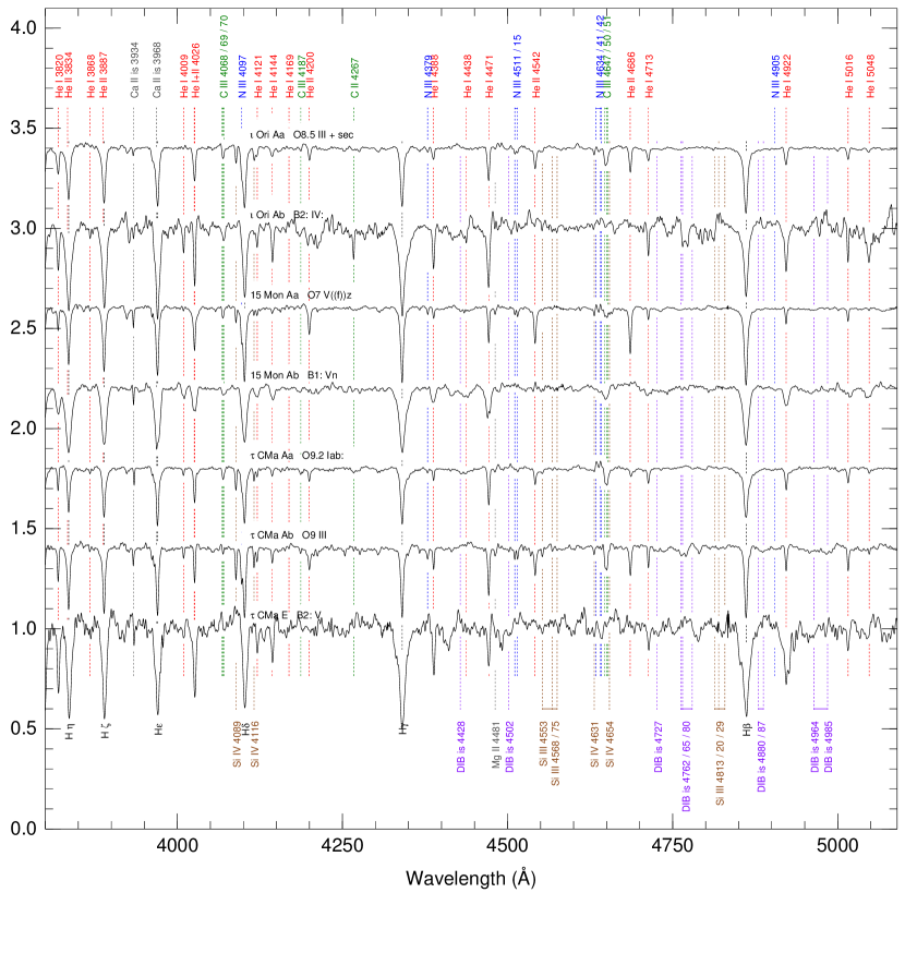
Figure 2: Extracted HST/STIS spectra. The velocity reference system is that of the star in each case and the spectra are plotted at a spectral resolution of 2500.

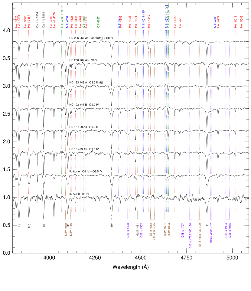
Figure 2: (Continued).

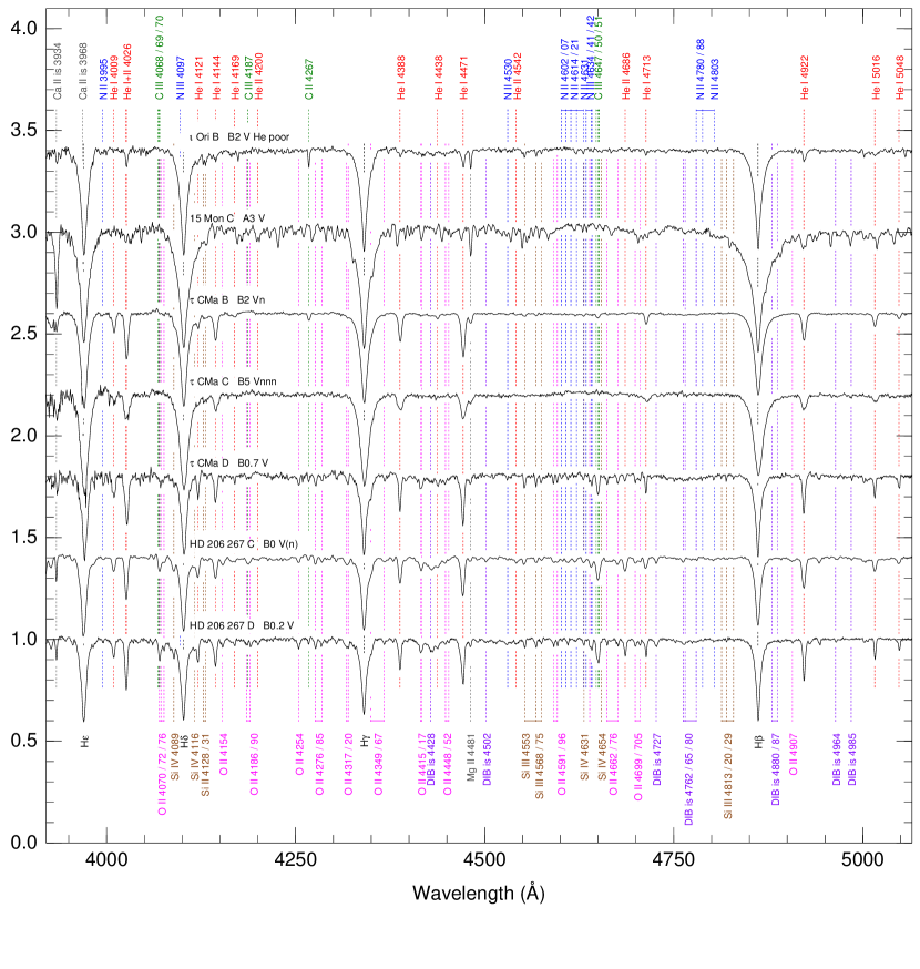
Figure 3: GOSSS spectra.

3.1 $\iota$ Ori Aa,Ab

 This system is composed of at least four stars. Two are in an eccentric 29.1 d period (Marchenko et al., 2000), form the visual component Aa, and were classified as O8.5 III + B0.2 V in MONOS-I. The previously spectroscopically unresolved Ab component is located 155 mas away. The more distant B component is 11$\aas@@fstack{\prime\prime}$3 away and is a He-poor B star (Conti & Loonen, 1970).

In our spectral extraction we fix $d^{\prime}$ between Aa and Ab to 155 mas (an estimate from the existing WDS values, which show the separation increasing between the mid 1990s and the last 2016 measurement), as the secondary is too weak to have its position in the spatial profile fitted simultaneously with the profile shape. The $\Delta B$ is the second largest in the HST/STIS sample after $\tau$ CMa Aa,E.

Some lines in Aa are slightly asymmetric but not to a sufficient degree as to allow us to give a spectral classification to the secondary spectroscopic component. The primary is clearly O8.5 III, as in MONOS-I. A second epoch may be able to provide a spectral classification for the secondary if the velocity separation is more favorable.

The Ab spectrum is one of the noisiest one in Fig. 2, as expected from the large $\Delta B$, but is clearly distinct from that of Aa. There are strong He i lines, no He ii lines or C iii $\lambda$4650 (making it B1 or later), and C ii $\lambda$4267 is strong (while absent in Aa), which is typical around B2. The Balmer lines are somewhat narrower than those of a dwarf at that subtype, hence the B2: IV: classification.

We also analyze here the GOSSS spectrum of the B component, a star with a very low $v\sin i$ and a number of corresponding narrow lines, which is relatively unusual among mid-B dwarfs, whose spectrum usually has few features. The simultaneous detection of the Si ii $\lambda\lambda$4128+31 doublet and the Si iii $\lambda\lambda\lambda$4553+68+75 triplet allows for a precise determination of the spectral subtype as B2 independently of any composition anomalies. The strength of C ii $\lambda$4267, Mg ii $\lambda$4481, and several weak N ii lines confirm the spectral subtype. At the same time, the Balmer line profiles correspond to a dwarf luminosity class for a B2 star. The big discrepancy lies in the He i lines, which are very weak when at B2 they should be very strong. Hence the He poor qualifier already noted half a century ago (Conti & Loonen, 1970). Note that Simbad lists a variety of spectral types for $\iota$ Ori B, the reason being that if one pays attention just to He i $\lambda$4471, Mg ii $\lambda$4481, and the Balmer lines we could easily classify it as B8 III. A cautionary tale here is that if the S/N were lower or $v\sin i$ were larger we would easily miss most of the weak lines and think this object is a late-B star.

Summarizing the results from different sources, $\iota$ Ori is a hierarchical system (Tokovinin, 1997) composed of an O8.5 III + B0.2 V spectroscopic binary (Aa) with a mid-B star orbiting around them (Ab, classified here for the first time) and another one much farther away (B). The A component has an entry in Gaia DR2 but without a parallax. The B component, on the other hand, has a Gaia DR2 measurement of $\varpi=2.3839\pm 0.0810$ mas and a good-quality RUWE (renormalized unit weight error, Lindegren et al. 2018) of 1.07, which allows for a high-quality distance measurement. Using the self-gravitating isothermal Galactic vertical distribution prior of Maíz Apellániz (2001, 2005b) with the updated parameters of Maíz Apellániz et al. (2008) and correcting for a parallax zero point of $40\pm 10$ $\mu$as, we obtain a distance of $412^{+14}_{-13}$ pc. Therefore the three orbits have estimated semi-major axes of 0.38 AU (from the SB2 data and estimated masses), 70 AU, and 4600 AU (from $d$), respectively, noting the last two values can be significantly different if the orbits have orientations far from the plane of sky or high eccentricities. From the last two semi-major axes the periods are estimated around 87 a and 43 ka. The WDS lists a significant motion of Ab with respect to Aa over a period of 22 a with a $d$ that is currently increasing (something that agrees with the value measured here), suggesting a period of several centuries, so the orbit of Ab with respect to Aa appears to be inclined, eccentric, or both.

3.2 15 Mon Aa,Ab

 This object is the ionizing source of the H ii region NGC 2264 and is composed of an inner Aa,Ab pair with a period of 108$\pm$12 a (Maíz Apellániz, 2019) and a third B component at a distance of 3$\aas@@fstack{\prime\prime}$0. In Maíz Apellániz et al. (2018) we used lucky spectroscopy to assign separate spectral types of O7 V((f))z var to Aa,Ab and B2: Vn to B but we were not able to separate Aa and Ab when we aligned the slit along them. The Maíz Apellániz (2019) orbit indicates that the system passed through periastron in early 1996, achieved a minimum $d$ of 19-20 mas shortly afterwards, and that the separation has increased since then. The WDS lists a large number of additional components, many of them likely independent stars in the NGC 2264 cluster, of which the only one within 30″ of AaAb is C.

The predicted $d^{\prime}$ at the time of the HST observation from the Maíz Apellániz (2019) orbit was 135 mas but our fitted value is somewhat larger, 143 mas, suggesting that the latest ground-based observations may slightly underestimate it.

We classify Aa as O7 V((f))z as we already did in MONOS-I but dropping the var suffix as we currently only have a single HST epoch. The absorption lines are especially narrow, indicating a low $v\sin i$. The spectrum of the Ab component is generally well separated from that of Aa but a small contamination (or rather oversubtraction) is seen at the bottom of the He i $\lambda$4471 absorption line. An accurate classification cannot be attained because the object is a fast rotator but based on the absence of both He ii lines and C ii $\lambda$4267, the presence of weak Si iii $\lambda$4553, and the width of the Balmer lines we arrive at B1: Vn.

We also classify here the GOSSS spectrum of the weak C component. It is an A3 V star.

15 Mon is another hierarchical system composed of a central O star and two fast rotators of B spectral type. In Maíz Apellániz (2019) we derived a Gaia DR2 distance of $719\pm 16$ pc, which places the current values of $d$ as 103 AU and 2200 AU for Aa,Ab and Aa,B, respectively. The measured semi-major axis of the Maíz Apellániz (2019) Aa,Ab orbit is 112.5 mas (smaller than the current $d$, note that the orbit is quite eccentric), which corresponds to 81 AU.

3.3 $\tau$ CMa Aa,Ab,E

 $\tau$ CMa is our southernmost target and, for that reason, was not included in MONOS-I. This is a complex system composed of an inner spectroscopic binary with a 154.92 d period (Struve & Pogo, 1928; Struve & Kraft, 1954; Stickland et al., 1998) orbited by a visual companion for which the latest $d$ values in the WDS are in the 110-120 mas range. In addition, one of the components shows eclipses with a much shorter period of 1.282 122 d (van Leeuwen & van Genderen, 1997). Another dim component, E, is listed as 0$\aas@@fstack{\prime\prime}$94 away in the WDS but note that the current position angles for both the Aa,Ab and Aa,E pairs are offset by 180 degrees in the WDS, i.e., Ab is actually to the NW of Aa and E is to the W of Aa, as already pointed out by Aldoretta et al. (2015) and confirmed independently in unpublished AstraLux imaging (see Maíz Apellániz 2010) and in a short STIS imaging exposure obtained in the same orbit as our spectra. The WDS also lists another three additional components with larger $d$: B, C, and D. GOSSS gives a combined spectral classification of O9 II for Aa,Ab (Sota et al., 2014) which is consistent with the previous result from Walborn (1972).

In our spectroscopic data we measure $d^{\prime}=95$ mas for Aa,Ab, which is somewhat smaller than the previous values in the WDS. Nevertheless, those other values were obtained 6-10 years earlier and older ones are even larger (in the 1960s $d$ appears to have been around 200 mas), so it appears that the system has a significant inwards motion in the plane of the sky confirmed by our measurement. The separation along the slit we measure for Aa,E is 685 mas which, corrected for the 43^o misalignment deduced from the imaging data, yields a $d=937$ mas, consistent with the WDS value.

The most important result for $\tau$ CMa is that both the Aa and Ab components have O-type spectral classifications, something that is shown here for the first time, as the Stickland et al. (1998) analysis was for just an SB1 orbit. We classify the weaker Ab component as O9 III. The brighter Aa component is an O9.2 with an uncertain luminosity classification, as the He/He and Si/He criteria give different results, which is often the case when the spectrum is a composite of a late O and an early B star (e.g. compare the $\sigma$ Ori case in Sota et al. 2014 and in MONOS-I). Therefore, the spectroscopic binary is likely to be Aa but we require a second HST epoch to confirm this.

The spectrum of the E component is very noisy due to the large $\Delta B$ or, equivalently, to the short exposure time for its magnitude, as the STIS spatial profile yields little contamination from Aa,Ab at such large separations. We are only able to derive an uncertain B2: V classification.

We also analyze here the GOSSS spectrum of the D, B, and C components. They are three B dwarfs of progressively later subtypes: B0.7, B2, and B5, respectively, with their magnitudes increasing accordingly. They also follow a progression in $v\sin i$ from slow, to fast, and to very fast values. Indeed, $\tau$ CMa C has an nnn rotation index, which corresponds to a $v\sin i$ close to 500 km/s. Surprisingly for such a fast B-type rotator, there is no sign of emission in any Balmer line (including H$\alpha$, observed but not shown here) so it does not appear to be a Be (at least when we observed it, Be emission lines can notoriously appear and disappear).

$\tau$ CMa is a high-order multiple system which is the brightest object at the core of the NGC 2362 cluster. As in other similar cases (e.g. HD 93 129 in Trumpler 14), it is difficult to say where the multiple system ends and the cluster begins and only long-term monitoring may provide an answer to that question…or it may not, as such circumstances may lead to unstable arrangements with exchanges of partners and/or ejections during the lifetime of the cluster, in which case the question may be ill posed. The Gaia DR2 RUWE for $\tau$ CMa Aa,Ab is 33.6, so we cannot use its parallax (which is negative, anyway) to estimate its distance. Instead, we use a simplified version of the algorithm of Maíz Apellániz (2019) to select the eight brightest stars in NGC 2362 (excluding $\tau$ CMa Aa,Ab) with similar proper motions and obtain a cluster parallax of $0.6265\pm 0.0477$ mas. Applying the same parallax zero point correction and prior as before, we obtain a distance of $1.50^{+0.12}_{-0.10}$ kpc to the cluster.

3.4 HD 206 267 Aa,Ab

 This is another complex system. The brightest component, Aa, is an SB2 with a 3.71 d period (Raucq et al., 2018). The Ab and B components were measured to be 100 mas and 1$\aas@@fstack{\prime\prime}$8 away, respectively, in MONOS-I but B is too faint to make a significant contribution to the spectrum. Two other bright components, C and D, are farther away. In MONOS-I we give a spectral classification of O6 V(n)((f)) + B0: V for Aa,Ab and note that at least one of the spectral types must be a composite given the presence of three early-type stars in the aperture.

In our spectroscopic data we measure $d^{\prime}=64$ mas and $\Delta B=0.95$ for Aa,Ab. The separation is significantly smaller than the previous AstraLux (Maíz Apellániz et al., 2019) and WDS values and the short STIS imaging exposures we took in the same orbit as the spectroscopy show the two stars aligned on the slit within $\sim 10^{\rm o}$, so a large position angle difference can be discarded. The magnitude difference is also smaller than the one measured with AstraLux but closer to the 1.1-1.3 mag values of the most recent WDS data. We have revised the Maíz Apellániz et al. (2019) data and we think that it is at fault due to the lack of adequate PSF stars (the problem does not affect the rest of the objects in that paper). Therefore, the separations and magnitude differences for HD 206 267 Aa,Ab in that paper should not be used but the position angles are more likely to be reliable, as those depend less on the PSF choice. In any case, the value of $d^{\prime}=64$ mas is clearly smaller than the previous HST value of 97.1 mas (a lower limit) from a 2008 FGS measurement by Aldoretta et al. (2015), indicating that there is a significant motion in the 11 a between the two epochs and that the period may be of the order of one or two centuries, as already suggested by Maíz Apellániz et al. (2019) from the change in position angle.

Our separate spectra confirms that the SB2 is indeed Aa, which was caught at an orbital point with a large velocity difference that allowed the two spectroscopic components to be classified. The system is O5 V((fc)) + B0: V. The primary of the spectroscopic binary is one spectral subtype earlier than the MONOS-I result (which was likely blended with Ab) and half a spectral subtype than the Raucq et al. (2018) result.

The Ab component, on the other hand, is classified as O9 V. This is the first time this object is directly classified, as previous studies had just guessed its nature.

We also analyze here the GOSSS spectra of the C and D components. Both are very early B-type dwarfs, B0 in the case of C and B0.2 in the case of D. The first one is a moderately fast rotator and the second one is a slow rotator.

HD 206 267 Aa,Ab is another high-order multiple system at the center of a cluster, in this case Trumpler 37. The Gaia DR2 RUWE for HD 206 267 Aa,Ab is 2.8, so we cannot use its parallax (which has a relatively large uncertainty, anyway) to estimate its distance. Instead, we use the parallaxes of the C and D components to obtain a combined value of $0.8807\pm 0.0516$ mas, where the uncertainty includes the covariance term. Applying the same parallax zero point correction and prior as before, we obtain a distance of $1093^{+67}_{-59}$ pc to HD 206 267.

3.5 HD 193 443 A,B

 This object is a triple system composed of a spectroscopic binary with a 7.467 d period (Mahy et al., 2013) and a visual companion located 137.7 mas away (Aldoretta et al., 2015). HD 193 443 A,B is a poorly known system, in part because of the confusion induced by the small $\Delta m$ between the two visual components A and B. In contrast with previous results, Aldoretta et al. (2015) found out a magnitude difference of $-$0.264 i.e. the A (currently eastern) component is dimmer than the B (currently western) component. Mahy et al. (2013) classified this system as O9 III/I + O9.5 V/III but failed to notice the presence of a third light in the system, so it is not clear from their results whether the spectroscopic binary is A or B. Sota et al. (2011, 2014) could only provide a combined spectral classification of O9 III for A,B.

As the WDS data suggests that the A,B pair is moving in a clockwise direction (position angles of 290-300^o in the early 20th century to 258.5^o in the late 2008 measurement of Aldoretta et al. 2015), we set the position angle of our slit at 250^o. We obtain a $d^{\prime}=138$ mas and $\Delta B=-0.26$ mag, which are nearly identical to the Aldoretta et al. (2015) results.

The derived spectral classifications for A and B are O8.5 III((f)) and O9.2 IV, respectively. No double lines are seen in either spectra but this was expected, as the maximum velocity separation for the eccentric spectroscopic orbit is not large and the system was caught near the quadrature that takes place far from periastron. We plan to observe it again at a more favorable epoch close to the other quadrature. Nevertheless, at the original spectral resolution some of the Ab lines are asymmetric, indicating that is the spectroscopic binary. If that were indeed the case, A would be the more massive, luminous, and evolved component but would be dimmer than B due to the existence of two stars there. What we can discard is that any of the stars is a supergiant, one of the possibilities mentioned by Mahy et al. (2013).

Somewhat differently from some of the previous cases, there are few objects associated with this system. The WDS lists a weak C component 9″ away with a Gaia DR2 proper motion consistent with being associated with A,B. There is no surrounding cluster, though, and some of the brighter nearby stars have differing proper motions. This poses a problem for calculating the distance to HD 193 443, as the Gaia DR2 entries for A,B and C have RUWE values of 14.2 and 2.8, respectively, making their parallaxes useless for a reliable determination. For this object we will have to wait at least until future Gaia data releases.

3.6 HD 16 429 Aa,Ab

 HD 16 429 is another complex system with an inner pair Aa,Ab separated by 0$\aas@@fstack{\prime\prime}$28 in MONOS-I and with a significant inwards relative motion. Farther away we find B, a foreground interloper with an F spectral type, and C, classified as B0.7 V(n) (see MONOS-I). Ab was measured to be fainter than Aa by 2.1-2.2 mag in MONOS-I. McSwain (2003) detected the existence of a spectroscopic binary in Aa,Ab and gave the three spectral types O9.5 II + O8 III-V + B0 V?, assigning the first one to Aa and the other two to Ab. In MONOS-I we pointed out that such a configuration was difficult to reconcile with the relatively large magnitude difference. The GOSSS data of Sota et al. (2014) was insufficient to resolve any components and provided only a combined spectral classification of O9 II-III(n) Nwk for Aa,Ab.

In the STIS spectra we measure $\Delta B=2.02$ mag and $d^{\prime}=275$ mas for the Aa,Ab pair, values that are compatible with the MONOS-I results and confirm that the two components are approaching each other.

We obtain a spectral classification of O9.2 III for Aa and of O9.5 IV for Ab. We do not see double or even asymmetric lines in either object, indicating we caught it far from either quadrature, which is consistent with the orbital phase predicted by the McSwain (2003) analysis. The first classification is relatively similar to the McSwain (2003) but the second one is considerably later than her result. One possibility would be that indeed Ab is the spectroscopic binary and our O9.5 classification is just a composite between earlier- and later-type stars. There are two issues with that. The first one is the previously mentioned magnitude difference, which makes it hard to accommodate two O/early-B stars in Ab and just one in Aa. The second one are the velocities. McSwain (2003) obtains a systemic velocity of $-$50 km/s for HD 16 429 Aa,Ab and that is close to the value we measure for Ab. On the other hand, for Aa we obtain a value close to $+$20 km/s. Therefore, the evidence points towards Aa being the spectroscopic binary. To confirm this we plan to obtain additional STIS epochs of the system.

The literature lists HD 16 429 as a multiple system but the Gaia DR2 data hints at the existence of a small cluster associated with it, as there are several stars that appear to follow a young isochrone at the same distance. We cannot use the Gaia DR2 data for Aa,Ab itself because, as with most of the systems in this paper, the unaccounted visual multiplicity in the Gaia pipeline translates into a large RUWE value. On the other hand we cannot use the data for the B component because it is a foreground chance alignment. The C component is a more promising candidate and appears to be the brightest member of the cluster with good quality data. As we did for $\tau$ CMa, we use a simplified version of the algorithm of Maíz Apellániz (2019) to select the three brightest stars in the vicinity (using C as the reference) with similar proper motions and obtain a cluster parallax of $0.4657\pm 0.0480$ mas. Applying the same parallax zero point correction and prior as before, we obtain a distance of $2.04^{+0.23}_{-0.19}$ kpc to the cluster.

3.7 IU Aur A,B

 The final target in our sample is also complex. The inner pair A,B is separated by 128-144 mas in the MONOS-I AstraLux data with a trend that suggests that the two components are approaching each other. Two weak (C and D) components are detected with AstraLux farther away. The A component is an eclipsing binary with relatively deep and similar primary and secondary eclipses (Özdemir et al., 2003). MONOS-I measured a variable magnitude difference between A and B of 1.40-2.06 mag, with most of the variation likely caused by the eclipses. The period of the eclipsing binary is 1.811 d (Drechsel et al., 1994) but the eclipses are modulated by an eccentric orbit with a 293.3 d period (Özdemir et al., 2003) which must be caused by a dim or dark object distinct from A and B that does not cause a significant signal in the observed spectrum (see MONOS-I). In MONOS-I we found that the primary apparently changes its spectral type between O8.5 III(n) and O9.5 IV(n) while the secondary also changes (but to a lesser degree) between O9.7 IV(n) and O9.7 V(n) but we cautioned that those changes may be caused not only by the proximity between the two stars and its associated orbital effects (Harries et al., 1998) but also by the different degrees of contamination by the B component.

The STIS spectra yield a $\Delta B$ of 2.04 mag but we had to fix $d^{\prime}$ due to the large $\Delta B$. The system was caught near quadrature, so we may consider that to be the uneclipsed magnitude difference, which agrees with the AstraLux results in MONOS-I.

Being able to eliminate the effect of the B component, we classify A as O8 IV(n) + O9.5 IV(n). As we suspected, the B component was making the two stars in the eclipsing binary appear as having a later spectral type.

The spectrum of the B component is relatively noisy but it is well separated from that of A, as all the lines have a single kinematic component in clear contrast to the two seen in A with a separation of $\sim$475 km/s. The derived spectral type is B1: V.

There are several massive stars (e.g. HD 35 619) and H ii regions close to IU Aur but it is not clear whether our target is associated with any of them. The bad quality of the Gaia DR2 astrometric fit (RUWE of 9.9) impedes the determination of its distance. As it was the case for HD 193 443, we will have to wait for future Gaia data releases.

4 Analysis and future work

 In this paper we have used HST/STIS to obtain spatially resolved spectroscopy of the close components of seven visual multiple systems containing at least one O star. We have failed to spatially resolve an eighth system, $\zeta$ Ori Aa,Ab, which is located in the most difficult region of the $d-\Delta B$ plane (Fig. 4). Previously, we had similarly resolved five similar systems using ground-based lucky spectroscopy with the WHT (Maíz Apellániz et al., 2018). Since then, we have used the same WHT setup to successfully separate several tens of similar systems (Maíz Apellániz et al. in preparation). In Fig. 4 we show the location of all those systems in the $d-\Delta B$ plane along with tentative empirical boundaries for each of the two techniques: HST/STIS and lucky spectroscopy with WHT/ISIS. Even though they are not plotted, we have attempted and failed to separate with lucky spectroscopy several targets located in the region between the two boundaries (see section 3.2 for an example).

As expected, both techniques can reach the smallest separation when the magnitude difference is small, a pattern that is repeated for every technique that attempts to resolve closely separated point sources and that depends on how narrow and stable the PSF is. Also as expected, HST/STIS provides a significant improvement in separation with respect to lucky spectroscopy, which we can quantify as a factor of $\approx 8$ (at the same $\Delta B$). This happens because the STIS PSF is narrower and more stable, being adequately defined by a diffraction pattern with slight modifications from small focus changes. In lucky spectroscopy, the PSF depends on the observing conditions (which are not always optimal) and even when seeing is exceptional there are wings that hamper the measurement of weak companions. Nevertheless, lucky spectroscopy has some advantages with respect to HST/STIS, namely the smaller fraction of time spent on overheads, the higher number of photons collected per final unit time (with the corresponding increase in S/N), and being a cheaper technique that allows for larger samples.

Another lesson of this work is that the Gaia DR2 astrometric results of unresolved multiple systems are suspect. This is a well known effect when the companion is a dark object (Andrews et al., 2019; Simón-Díaz et al., 2020) but it is also noticeable when there are two or more moving bright objects blended into a Gaia source, which is the case for a majority of the O stars in the Galaxy given the limitations of the telescope (Brandeker & Cataldi, 2019). An advice here is that one should not analyze data from the Gaia archive without reading the fine print e.g. using the RUWE to estimate the validity of the astrometry. The situation should change in the future when the Gaia epoch astrometry is released, as one would be able to fit stars of interest with binary parameters, possibly constrained by external information such as spectroscopic or visual orbits.

We still have twelve remaining visits in HST GO program 15 815 that will be used to observe two more systems ($\theta^{1}$ Ori Ca,Cb and HD 193 322 Aa,Ab) and obtain new epochs for some of the targets in this paper. We also plan to request more HST time to extend the sample to other massive stars with close visual companions. Finally, we want to extend the lucky spectroscopy technique to other ground-based telescopes. Overall, in the next few years we hope to obtain spatially resolved spectroscopy of $\sim$100 visual binaries and, in that way, significantly improve our statistics of such systems.

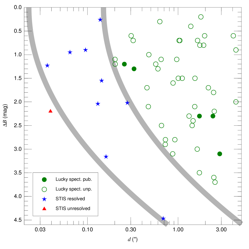
Figure 4: Binary systems resolved using lucky spectroscopy with WHT/ISIS (published in Maíz Apellániz et al. 2018 and unpublished) and HST/STIS and unresolved systems using HST/STIS in the $d-\Delta B$ plane. The gray curves mark the tentative empirical boundaries between the regions in the plane accessible with different techniques: the left one is for HST/STIS and the right one for lucky spectroscopy with WHT/ISIS.