Hydrodynamics of quartz crystal microbalance experiments with liposome-DNA complexes

Abstract

The quartz crystal microbalance (QCM) is widely used to study surface adsorbed molecules, often of biological significance. However, the relation between raw acoustic response (frequency shift $\Delta f$ and dissipation factor $\Delta D$) and mechanical properties of the macromolecules still needs to be deciphered, particularly in the case of suspended discrete particles. We study the QCM response of suspended liposomes tethered to the resonator wall by double stranded DNA, with the other end attached to surface-adsorbed neutravidin through a biotin linker. Liposome radius and dsDNA contour length are comparable to the wave penetration depth ($\delta\sim 100\ \mathrm{nm}$). Simulations, based on the immersed boundary method and an elastic network model for the liposome-DNA complex, are in good agreement with experimental results for POPC liposomes. We find that the added stress at the resonator surface, i.e. the impedance Z sensed by QCM, is dominated by the flow-induced liposome surface-stress, which propagates towards the resonator by viscous forces. QCM signals are extremely sensitive to the liposome’s height distribution P(y) which depends on the actual number and mechanical properties of the tethers, in addition to the usual local attractive/repulsive chemical forces. Our approach helps in deciphering the role of hydrodynamics in acoustic sensing and revealing the role of parameters hitherto largely unexplored. A practical consequence would be the design of improved biosensors and detection schemes.

The quartz crystal microbalance (QCM) is a technique for research at interfaces with applications ranging from nanotribology and soft matter to biology, health care and environmental monitoring Krim (2012); Johannsmann (2015); Bragazzi et al. (2015); Rodahl et al. (1997), covering a range of length-scales from nanometers to tens of microns. In biophysics-related research, QCM with dissipation monitoring (QCM-D) operates in liquids and follows real-time changes in assemblies of lipid membranes, DNA, proteins, nanoparticles, viruses and cells Rodahl et al. (1997); Reviakine et al. (2011); Keller and B. (1998); Tsortos et al. (2016); Saitakis and Gizeli (2012); Tellechea et al. (2009). In a QCM experiment, the analytes form the interface between the solid substrate (a quartz crystal piezoelectric resonator) and the liquid environment (water) where they are typically exposed to $5-150\,\mathrm{MHz}$ transverse oscillations; the sensor monitors, in real time, minute variations in the resonance frequency $f$ and energy dissipation factor $D$ (or decay rate $\Gamma=Df/2$). In vacuum and for rigid films the Sauerbrey relation Sauerbrey (1959) indicates that the inertia of the deposited mass will reduce the resonator frequency proportionally to $\Delta f/f$ ; for a resolution of $0.1\ \mathrm{Hz}$ this results in an extremely small limit of detection of $10^{-12}\mathrm{g/cm^{2}}$ . In a liquid, viscous forces propagate the resonator’s transverse oscillations up to 3 times the penetration depth $\delta=(2\eta/\rho\omega)^{1/2}\in[36,197]\mathrm{nm}$, leading to the so-called Stokes flow; here, $\omega=2\pi f$ while $\eta$ is the fluid viscosity and $\rho$ its density. In the case of a purely viscous Newtonian fluid the shifts $\Delta f$ and $\Delta D$ were derived by Kanazawa and Gordon Kanazawa and Gordon (1985) and subsequent works Ricco and Martin (1987). Johannsmann Johannsmann et al. (1992) and Voinova Voinova et al. (1999) later used effective-medium theory and phenomenological constitutive relations to estimate viscoelastic properties of the assumed film-formations of the material covering the sensor surface. Lately, experiments with discrete particles such as liposomes and viruses made use of a different approach providing estimations of the size of the nanoentities involved Tellechea et al. (2009). A model developed by Tsortos Tsortos et al. (2016, 2008); Raptis et al. (2019) allowed for quantitative size and shape evaluation of biomolecules (DNA, proteins) Papadakis et al. (2010); Mateos-Gil et al. (2016); here, the hydrodynamic quantities of intrinsic viscosity $[\eta]$ and radius $R_{h}$ were explicitly taken into account and were linked to the acoustic ratio $\Delta D/\Delta f$ Tsortos et al. (2008). When the limit of detection for an analyte is of importance (e.g. in biotechnology and in medical applications), the formation of molecular complexes at the surface is one way to enhance the QCM signal. Signal-enhancers typically of O(100) nm, such as liposomes, magnetic beads and gold nanoparticles are anchored to the analyte and thus suspended in the fluid, tens of nanometers away from the sensor surface. Viscoelastic film theories based on 1D equations, substantially fail to provide useful information on these and other discrete-particle settings Johannsmann (2015); Reviakine et al. (2011).

A theoretical understanding of such systems requires a solid hydrodynamic analysis, involving 3D unstationary flow patterns resulting from the viscous propagation of the fluid-induced forces acting on the solutes. Numerical studies of QCM hydrodynamics of discrete particles qualitatively reproduce experimental observations, such the coverage dependence of $\Delta D/\Delta f$, providing preliminary answers to a large list of still unexplained phenomenaJohannsmann (2015). These studies Reviakine et al. (2011); Tellechea et al. (2009) carried out in 2D using the commercial package COMSOL and more recently in 3D using lattice Boltzmann solvers Johannsmann and Brenner (2015); Gillissen et al. (2018), considered adsorbed rigid particles at fixed positions (obstacles). However, fixing the particle position introduces ad-hoc forces into the fluid (those required to keep the ‘obstacle’ fixed), which alter the measurement of the system impedance. A correct representation of QCM hydrodynamics requires solving the dynamics of the analytes, including the fluid traction acting on them and other interactions (inter-particle forces, surface or contact forces and advection due to a mean flow, if required); evidently, this issue is particularly important in the case of suspended particles. In this Letter we present an experimental and theoretical study of the QCM response of individual liposome-DNA complexes. Simulations are carried out with a finite volume fluctuating hydrodynamic solver equipped with the immersed boundary method, which describes the particle dynamics and uses an elastic network model to reproduce molecular mechanical properties (e.g. bending rigidity). The good agreement with experiments (carried out with POPC liposomes) allows us to affirm that the analyte impedance is strongly dominated by the hydrodynamic perturbation created by the liposome, which is suspended in the liquid and tethered by a DNA strand (Fig. 1).

Experiments. Liposome-DNA (LDNA) complexes were formed by sequential injections of neutravidin (NAv), DNA, and liposomes; more details in Supplementary Information (SI). dsDNA with 21, 50 and 157 base pairs (bp) having lengths $L_{\mathrm{DNA}}$ $7$, $17$ and $53\mathrm{nm}$, respectively, were used. Liposomes of radius of 15, 25, 50 and 100 nm were considered. In order to be captured by the NAv layer previously formed on the surface, DNA fragments bear a biotin at one end. In addition, a cholesterol was incorporated to the opposite DNA end for subsequent liposome binding due to its strong affinity for the lipid membrane. Ring-down QCM experiments were performed with an E4-Qsense (Biolin, Sweeden) device at $T=25^{o}C$ under continuous flow velocity of 60 $\mu\mathrm{L/min}$. Measurements of $\Delta f$ and $\Delta D$ based on the ring-down approach have been described elsewhere Rodahl et al. (1995). Briefly, after excitation pulses separated by milliseconds, a crystal sensor resonator performs underdamped oscillations described by $x(t)=x_{0}\exp[-\Gamma t]\cos[2\pi ft+\phi]$, where $x_{0}\approx 2\mathrm{nm}$, and $\Gamma$ and $f$ depend on the acoustic response related to the sensor loading. The decay rate $\Gamma$ is often expressed in terms of the “dissipation factor”, $D=2\Gamma/f_{n}$. The fundamental frequency of the particular cut of the quartz crystal is $f_{0}=5\mathrm{MHz}$ and here we report experimental results for the seveth harmonic $f_{7}=35\mathrm{MHz}$. QCM experiments monitor the time evolution of the acoustic signal registering the changes in frequency ($\Delta f$) and dissipation ($\Delta D$) upon successive sample injections and surface binding of NAv, DNA and liposomes (Fig. S1). These shifts increase with the amount of deposited material. To get an intensive quantity the procedure consists in plotting the acoustic ratio $-\Delta D/\Delta f$ against $\Delta f$ and extrapolating it to the limit of an infinitesimally small load: this defines the so called dissipation capacity $\mathrm{DC}=-\lim_{\Delta f\rightarrow 0}\Delta D/\Delta f$. The minus sign is convenient because an extra load usually implies $\Delta f<0$ and $\Delta D>0$ which, following the analogy with an overdamped spring Johannsmann (2015), are commonly intrepreted as extra “mass” ($\Delta f$) and “dissipation” ($\Delta D$).

Impedance analysis. Our numerical analysis is based on the well established small load approximation (SLA) Johannsmann (2015) which relates the impedance, $\mathcal{Z}=\hat{\sigma}/v_{0}$ (ratio of the wall stress and the surface velocity) to the complex frequency shift $\Delta\tilde{f}=\Delta f+i\Delta\Gamma$ measured in ring-down experiments. The SLA is valid if the resonator’s mass per unit area is much larger than the load, which is a safe approximation in our case (where $\Delta f/f_{0}\sim 10^{-5}$ or even less). The impedance of the complex load is expressed as the sum of $\mathcal{Z}=\mathcal{Z}^{(Q)}+\mathcal{Z}^{(0)}+\mathcal{Z}^{(\mathrm{DNA})}+\mathcal{Z}^{(\mathrm{LDNA})}$, where the impedances correspond, respectively, to the clean quartz resonator $\mathcal{Z}^{(Q)}$, the (unloaded) Newtonian solvent $\mathcal{Z}^{(0)}$ Kanazawa and Gordon (1985) the DNA strand without a liposome $\mathcal{Z}^{(\mathrm{DNA})}$ and, the LDNA impedance $\mathcal{Z}^{(\mathrm{LDNA})}$. For any contribution (different from $Q$), the SLA yields Johannsmann (2015) $\Delta\tilde{f}^{(a)}/f_{0}=\mathrm{i}\mathcal{Z}^{(a)}/(\pi\mathcal{Z}^{(Q)})$, where $\mathcal{Z}^{(Q)}=8.8\times 10^{6}\ \mathrm{kg/(m^{2}s)}$. The real part of $\mathcal{Z}^{(a)}$ is related to the dissipation and the imaginary part to the frequency shift ($\mathrm{Re}[\mathcal{Z}^{(a)}]=\mathcal{Z}_{R}\propto-\Delta\Gamma$ and $\mathrm{Im}[\mathcal{Z}^{(a)}]=\mathcal{Z}_{I}\propto-\Delta f$) while the acoustic ratio is $\mathrm{DC}^{(a)}=-2\mathcal{Z}_{R}^{(a)}/(\mathcal{Z}_{I}^{(a)}f_{n}[\mathrm{MHz}])$, and $f_{n}$ is the working frequency (here $n=7$).

Simulations. Our mesoscopic model is based on a fluctuating hydrodynamic solver for compressible unsteady flow equipped with the immersed boundary method to couple fluid and structure dynamics Usabiaga et al. (2013, 2014); Balboa-Usabiaga . It is implemented in the GPU code FLUAM (FLuid And Matter interaction), a second-order accurate finite volume scheme on a staggered grid Balboa et al. (2012) of side $h$. The liposome and dsDNA are represented using beads of radius $h$ (Fig. 1) connected by harmonic springs and/or bending potentials (see SI). An elastic network is used to model the membrane of the (hollow) liposome by connecting nearest neighbours of the network with harmonic springs: the bonding force ${\bf F}_{ij}=-k_{L}({\bf r}_{ij}-r_{0})$ includes the equilibrium distance $r_{0}\approx h$ and the spring constant $k_{L}$ determining the liposome rigidy. Here we consider the rigid limit (high $k_{L}$) to focus on the leading impedance contribution. The double stranded DNA (dsDNA) is modelled by a bead model for semiflexible polymers, with bending energy extracted from the DNA persistence length at room temperature (50 nm). We shall use the term link to denote the DNA-wall force $F_{\mathrm{link}}$.

The geometry is illustrated in Fig. 1. The simulation box is periodic in the resonator plane $x-z$, with dimensions $L\times L_{y}\times L$. Rigid no-slip walls at $y=0$ and $y=L_{y}$ are imposed via explicit boundary conditions Usabiaga et al. (2013); Usabiaga (2014)). The top wall is kept at rest while the bottom wall at $y=0$ moves in the $x$ direction with velocity $v_{wall}=v_{0}\cos(2\pi ft)$ with $v_{0}$ set to fix a small wall displacement $x_{0}<h$. To achieve the required numerical convergence we used a spatial resolution of $h=3.958\ \mathrm{nm}$ (see SI). The code units map the density and kinematic viscosity of water at $T=25^{o}\,\mathrm{C}$ (see SI). The sound velocity $c$ was set to match the experimental value of the group $f_{7}\delta/c\sim 3\times 10^{-3}$, whose smallness indicates a minor effect of fluid-compressibility Mazur and Bedeaux (1974). Moreover, the large time scale separation between liposome diffusion time and the QCM oscillation period ($6\pi\eta R^{3}f/k_{B}T>10^{4}$) makes it possible to neglect thermal fluctuations over the short simulation runs we used to evaluate the impedance (about 10 periods). We stress, however, that in our simulations the liposome is free to move according to the flow traction; this is essential to obtain unbiased results, particularly because the liposomes are not adsorbed but suspended.

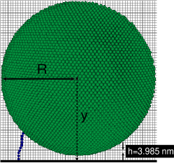
Figure 1: Snapshot of the numerical model of a liposome of $R=100\ \mathrm{nm}$ radius tethered to a DNA strand attached to the resonator wall (see text). The coupling between the analyte and the fluid dynamics is solved using the immersed boundary method (IBM) Usabiaga et al. (2013); Balboa-Usabiaga . The spatial resolution is set by the fluid cell size $h$ (here $3.958\mathrm{nm}$). The bottom wall oscillates transversally at $35\mathrm{MHz}$, with a small amplitude (less than one cell).

Computational protocol. An “instantaneous” value of $f$ and $D$ in the QCM experiment corresponds to an ensemble average over many LDNA assemblies over a large number of pulse-waiting time sequences (each one in the milisecond range). We average over a set of 40 initial equilibrium configurations extracted from Monte Carlo sampling of the LDNA complex (SI for details). The impedance of each configuration is measured running FLUAM over 10 periods, after the transient regime. We record the time-depedent wall stress $\sigma(t)=\sigma_{\mathrm{hydro}}+\sigma_{\mathrm{link}}$ with contributions from the DNA-wall link $\sigma_{\mathrm{link}}=F_{\mathrm{link}}/L^{2}$ and the wall hydrodynamic stress $\sigma_{\mathrm{hydro}}(t)=\eta\langle(\partial v_{x}({\bf r},t)/\partial y)_{wall}\rangle$ (angle brackets denote average over the whole surface). Setting $\sigma(t)=\mathrm{Re}[\hat{\sigma}\exp(-\mathrm{i}\omega t)]$ we obtain the stress phasor $\hat{\sigma}$ by fitting to $\sigma(t)=\mathrm{Re}[\hat{\sigma}]\cos(\omega t)+\mathrm{Im}[\hat{\sigma}]\sin(\omega t)$. This provides the total impedance $\mathcal{Z}=\hat{\sigma}/v_{0}$ of each initial configuration. The LDNA impedance is $\mathcal{Z}^{(\mathrm{LDNA})}=\mathcal{Z}-\mathcal{Z}^{(0)}-\mathcal{Z}^{(\mathrm{DNA})}$, where $\mathcal{Z}^{(0)}=(\mathrm{i}-1)\,\eta/\delta$ corresponds to the unperturbed (Stokes) flow and $\mathcal{Z}^{(\mathrm{DNA})}$ to the DNA anchor (without liposome) which was found to be negligible.

Calculations of $\mathcal{Z}^{(\mathrm{LDNA})}$ were carried out for increasing box side $L$ (the coverage being $\phi=1/L^{2}$). Although a periodic array of a single analyte is far from the experimental randomness, the variation of $\Delta D/\Delta f$ with $\phi$ is similar to that observed in experiments (see SI). Consistently, in simulations, the dissipative capacity is defined as the value of the acoustic ratio in the limit of low coverage $\mathrm{DC}_{num}=-\lim_{\phi\rightarrow 0}2\mathrm{Re}[\mathcal{Z}^{(\mathrm{LDNA})}]/(\mathrm{Im}[\mathcal{Z}^{(\mathrm{LDNA})}]f_{n})$.

Results. Numerical and experimental estimations of the acoustic ratio $\mathrm{DC}\equiv\mathrm{DC}^{\mathrm{(LDNA)}}$ are compared in Fig. 2, both showing an increase of $\mathrm{DC}$ with the liposome radius $R$ and the DNA contour length $L_{\mathrm{DNA}}$. The agreement is quite close to being quantitative and gives us confidence to deploy our model in future efforts to gradually understand the large number of factors affecting the value of $\mathrm{DC}$ (some of them will be mentioned below). Such a task demands a theoretical analysis of the impedance, presented below.

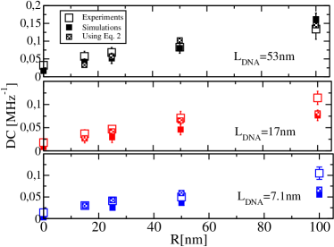
Figure 2: Dissipative capacity of liposome-DNA complexes at frequency $f_{n}=35\ \mathrm{MHz}$, against the liposome radius $R$ for different dsDNA contour lengths Filled symbols correspond to simulation results, crossed symbols to Eq. 2 (using Eq. 1 for $\mathcal{Z}^{(\mathrm{L})}$) and open symbols to experiments using POPC liposomes at $T=25^{o}$C Milioni et al. (2020). Simulations were performed with a mesh of $h=3.958\ \mathrm{nm}$ in boxes of $L=506.6\ \mathrm{nm}$ side.

Analysis. The impedance of the LDNA assembly can be decomposed into contributions from the liposome $(L)$ and the DNA $\mathcal{Z}^{(\mathrm{LDNA})}=\mathcal{Z}^{(\mathrm{LDNA})}_{L}+\mathcal{Z}^{(\mathrm{LDNA})}_{\mathrm{DNA}}$. The term $\mathcal{Z}^{(\mathrm{LDNA})}_{\mathrm{DNA}}$ collects the contributions of the linker and the hydrodynamic impedance of the DNA. Note that with the exception of the small molecular linker (biotin), the DNA chain is suspended in the fluid and the dominant part of its impedance is of hydrodynamic origin. In general, the hydrodynamic impedance arises from the fluid-induced forces (or force distributions) on the solutes, which are transfered back to the fluid by momentum conservation and propagate by viscous diffusion to the resonator, creating stress on the wall. The lack of symmetry makes elusive an analytical approach to the fluid-induced dynamics, even for a point-particle under a Stokes flow A. et al. (2018). Fluid-induced forces could be of inertial origin (relative fluid-particle accelerations leading to a net force on the solute). However, due to the extremely small density constrast of the quasi-neutrally-buoyant liposomes and DNA, inertia is negligible. Even so, liposomes will bear a stress distribution at their surface due to their reaction against flow-induced deformation. The induced liposome surface stress, along with the line tension along the DNA, are propagated back to the wall by viscous transport. There, at the resonator, the only way to disentangle $\mathcal{Z}^{(\mathrm{LDNA})}_{L}$ from $\mathcal{Z}^{(\mathrm{LDNA})}_{\mathrm{DNA}}$ is to compare the impedance of a free-floating (not tethered) liposome $\mathcal{Z}^{(\mathrm{L})}$ with that of a LDNA assembly where the liposome is placed at a similar height $y$. This comparison, in Fig. 3, clearly shows that the dominant contribution to $\mathcal{Z}^{(\mathrm{LDNA})}$ comes from the liposome’s surface stress, determined by $\mathcal{Z}^{(\mathrm{L})}(y)$. Before analyzing the role of the DNA strand, we focus on $\mathcal{Z}^{(\mathrm{L})}(y)$ in Fig. 3. Remarkably $\mathcal{Z}^{(\mathrm{L})}(y)$ decays almost exponentially with $y$: this general trend can be explained by hydrodynamic reflection. Resonator vibrations (with velocity $v_{0}$) are propagated upwards to the fluid by viscous forces and creates the unsteady and distance-dependent Stokes flow. Its velocity field (phasor), $v_{0}\exp[-\alpha y]$, contains the viscous propagator ($\exp[-\alpha y]$, with $\alpha=(1-\mathrm{i})/\delta$). The behavior of $\mathcal{Z}^{(\mathrm{L})}(y)$ can be understood using a corollary of Faxén’s theorem (valid for steady Kim and Karrila (2013) and unsteady flow Pozrikidis (2016)), which guarantees that the solute’s surface stress is a linear function of the ambient flow. Far away from the resonator, the ambient flow is similar to the Stokes flow, so the liposome surface stress should scale as $\exp[-y\alpha]$. The stress reflects back to the surface by viscous forces leading to $\mathcal{Z}^{(\mathrm{L})}\sim Z_{S}\exp[-2\alpha y]$, where the prefactor $Z_{S}=(20\pi/3)\eta R^{3}/(L^{2}\delta^{2})$ is taken to be consistent with the stresslet of a sphere under steady shear . Close to the resonator, the ambient flow includes a significant contribution from the wall reaction field Felderhof (2012) and the impedance becomes a decreasing function of the surface-to-sphere distance $y-R$. This reasoning leads us to the following ansatz,

$$\mathcal{Z}^{(\mathrm{L})}(y)=Z_{S}\left[(A+\mathrm{i}B)\exp[-2\alpha y]+\frac{2\mathrm{i}C}{\alpha(y-R)}\right].$$ (1)

Using $A\approx 1.40(R/\delta)^{2}$, $B\approx 1.5-0.03\exp(2.5\,R/\delta)$ and $C\approx 0.01$ (see SI), Eq. 1 fits our numerical results for $y/\delta>0.04$ within less than $5\%$ error (see Fig. 3).

The contribution of the DNA can now be estimated as $\mathcal{Z}^{(\mathrm{LDNA})}_{\mathrm{DNA}}=\mathcal{Z}^{(\mathrm{LDNA})}-\mathcal{Z}^{(\mathrm{L})}$. As shown in Fig. S5, $\mathcal{Z}^{(\mathrm{LDNA})}_{\mathrm{DNA}}$ mildly increases with $L_{\mathrm{DNA}}$. Its imaginary part does not greatly vary with $R$ while its real part increases linearly with $R$. We find that the DNA represents a minor contribution to the total impedance $\mathcal{Z}^{(\mathrm{LDNA})}$ for $R>50\mathrm{nm}$, while it becomes noticeable for smaller liposomes (see SI).

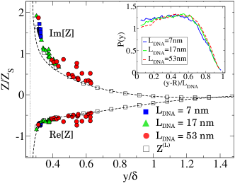
Figure 3: Impedance of a liposome of $R=25\ \mathrm{nm}$ versus the scaled wall distance $y/\delta$ (penetration length $\delta=95\,\mathrm{nm}$ for $f_{7}=35\ \mathrm{MHz}$). Open squares correspond to a freely suspended liposome ($\mathcal{Z}^{(\mathrm{L})}$) and filled circles to individual configurations of the liposome-DNA complex for several contour lengths. Results obtained in a square box of side $L=253,3\ \mathrm{nm}$ and mesh-size (resolution) $h=3.958\ \mathrm{nm}$. Dashed lines correspond to Eq. 1 (the vertical line indicates the wall). Inset: Monte Carlo results for the probability density of finding the liposome ($R=25\ \mathrm{nm}$) at height $y$. The scaled length $(y-R)/L_{\mathrm{DNA}}$ provides a master curve for all values of $L_{\mathrm{DNA}}$ (see SI).

Figure 3 shows that that the dispersion of $\mathcal{Z}^{(\mathrm{LDNA})}$ around its average decaying trend is relatively small and does not greatly vary with $y$. Thus $\mathcal{Z}^{(\mathrm{LDNA})}_{\mathrm{DNA}}$ does not strongly vary with the orientation of the DNA strand. The main effect of the DNA is to constrain the liposome position and, notably, to determine its height distribution $P(y)$. The average impedance is obtained from the weighted average,

$$\langle\mathcal{Z}^{(\mathrm{LDNA})}\rangle=\int P(y)\mathcal{Z}^{(\mathrm{LDNA})}(y)dy,$$ (2)

where $\mathcal{Z}^{(\mathrm{LDNA})}(y)=\mathcal{Z}^{(\mathrm{L})}(y)+\mathcal{Z}^{(\mathrm{LDNA})}_{\mathrm{DNA}}$. Relation 2 is extremely useful because it decomposes the analyte and anchor contributions, allowing for a fast evaluation of non-trivial effects. $P(y)$ encodes important microscopic information about the anchor: bending rigidity, linker-DNA tilt energy Wong and B. (2004) or large values of the DNA coverage Huang et al. (2010) which could lead to multiple anchors connected to the liposome Milioni et al. (2020)). In general, $P(y)$ can also introduce information into Eq. 2 about physico-chemical forces between the analyte and the wall (solvation, dispersion, electrostatic forces) as well as the effect of advection under a strong Poiseulle flow. All these effects are known to alter the acoustic ratio and their relevance can be tested using Eq. 2, by pre-evaluating $P(y)$, either theoretically or from Monte Carlo simulations (MC). We use MC sampling to obtain $P(y)$ for an electrically neutral liposome (POPC) anchored by a single DNA chain. The inset of Fig. 3 shows $P(y)$, which applied to Eq. 2 (fed with $\mathcal{Z}^{(\mathrm{L})}$ in Eq. 1 and $\mathcal{Z}^{(\mathrm{DNA})}_{\mathrm{DNA}}$) predicts values of DC quite close to experimental results (crossed symbols in Fig. 2).

We have shown that the acoustic response of suspended particles in QCM is mainly determined by the hydrodynamic response of the analyte, which strongly depends on its height distribution $P(y)$. The hydrodynamic response of liposomes also depends on their bending rigidity $\kappa$ and membrane fluidity Kim and Karrila (2013). Soft liposomes, with smaller $\kappa$ and higher fluidity, experimentally yield slightly smaller DC Milioni et al. (2020). A recent analytical study Melendez et al. (2020) indicates that both effects might be antagonistic (DC decreases with $\kappa$ but increases with fluidity). Disentangling all this subtle information hidden beneath the complex QCM hydrodynamic fields requires a combined effort of experiments, simulations and hydrodynamic theory. This work represents a step in this direction.

Acknowledgments. We acknowledge the EU Commision for the FET-OPEN CATCH-U-DNA project. R.D-B acknowledges support from MINECO via the proyect FIS2017-86007-C3-1-p.

References

- Krim (2012) Krim, J. Adv. Phys. 61(3), 155 (2012).
- Johannsmann (2015) D. Johannsmann, The Quartz Crystal Microbalance in Soft Matter Research, Fundamentals and modeling (Springer, 2015).
- Bragazzi et al. (2015) N. L. Bragazzi, D. Amicizia, D. Panatto, D. Tramalloni, I. Valle, and Gasparini, In Adv. Protein Chem. Struct. Biol. 101, 149 (2015).
- Rodahl et al. (1997) M. Rodahl, F. Hook, C. Fredriksson, C. A. Keller, A. Krozer, P. Brzezinski, M. Voinova, and B. Kasemo, Faraday Discussions 107, 229 (1997).
- Reviakine et al. (2011) I. Reviakine, D. Johannsmann, and R. P. Richter, Anal. Chem. 83(23), 8838 (2011).
- Keller and B. (1998) C. A. Keller and K. B., B. Biophys. J. 75, (3), 1397 (1998).
- Tsortos et al. (2016) A. Tsortos, G. Papadakis, and E. Gizeli, Analytical chemistry 88, 6472 (2016).
- Saitakis and Gizeli (2012) M. Saitakis and E. Gizeli, Cell. Mol. Life Sci 69 (3), 357 (2012).
- Tellechea et al. (2009) E. Tellechea, D. Johannsmann, N. F. Steinmetz, R. P. Richter, and I. Reviakine, Langmuir 25, 5177 (2009).
- Sauerbrey (1959) G. Sauerbrey, Zeitschrift fur Physik 155, 206 (1959).
- Kanazawa and Gordon (1985) K. K. Kanazawa and J. G. Gordon, Analytical Chemistry 57, 1770 (1985).
- Ricco and Martin (1987) A. J. Ricco and S. Martin, J. Appl. Phys. Lett. 50 (21), 1474 (1987).
- Johannsmann et al. (1992) D. Johannsmann, K. Mathauer, G. Wegner, and W. Knoll, Phys. Rev. B 46 (12), 7808 (1992).
- Voinova et al. (1999) M. V. Voinova, M. Rodahl, M. Jonson, and B. Kasemo, Phys. Scripta 59, 391 (1999).
- Tsortos et al. (2008) A. Tsortos, G. Papadakis, K. Mitsakakis, K. A. Melzak, and E. Gizeli, Biophysical journal 94, 2706 (2008).
- Raptis et al. (2019) V. Raptis, A. Tsortos, and E. Gizeli, Phys. Rev. Applied 11, (3), 034031 (2019).
- Papadakis et al. (2010) G. Papadakis, A. Tsortos, and E. Gizeli, Nano Lett. 10, 5093 (2010).
- Mateos-Gil et al. (2016) P. Mateos-Gil, A. Tsortos, M. Vélez, and E. Gizeli, Chemical Communications 52, 6541 (2016).
- Johannsmann and Brenner (2015) D. Johannsmann and G. Brenner, Analytical chemistry 87(14), 7476 (2015).
- Gillissen et al. (2018) J. J. Gillissen, J. A. Jackman, S. R. Tabaei, and N.-J. Cho, Analytical chemistry 90, 2238 (2018).
- Rodahl et al. (1995) M. Rodahl, F. Hook, A. Krozer, P. Brzezinski, and B. Kasemo, Review of Scientific Instruments 66, 3924 (1995).
- Usabiaga et al. (2013) F. B. Usabiaga, I. Pagonabarraga, and R. Delgado-Buscalioni, Journal of Computational Physics 235, 701 (2013).
- Usabiaga et al. (2014) F. B. Usabiaga, R. Delgado-Buscalioni, B. E. Griffith, and A. Donev, Computer Methods in Applied Mechanics and Engineering 269, 139 (2014).
- (24) F. Balboa-Usabiaga, FLUAM https://github.com/fbusabiaga/fluam/.
- Balboa et al. (2012) F. Balboa, J. B. Bell, R. Delgado-Buscalioni, A. Donev, T. G. Fai, B. E. Griffith, and C. S. Peskin, Multiscale Modeling & Simulation 10, 1369 (2012).
- Usabiaga (2014) F. B. Usabiaga, Ph.D. thesis, Universidad Autonoma de Madrid (2014).
- Mazur and Bedeaux (1974) P. Mazur and D. Bedeaux, Physica 76, 235 (1974).
- Milioni et al. (2020) D. Milioni, P. Mateos-Gil, G. Papadakis, A. Tsortos, O. Sarlidou, and E. Gizeli, (submitted) (2020).
- A. et al. (2018) S. A., M. J., and M. P. J., J. Fluid Mach. 841, 883 (2018).
- Kim and Karrila (2013) S. Kim and S. J. Karrila, Microhydrodynamics: principles and selected applications (Courier Corporation, 2013).
- Pozrikidis (2016) C. Pozrikidis, Fluid dynamics: theory, computation, and numerical simulation (Springer, 2016).
- Felderhof (2012) B. Felderhof, Physical Review E 85, 046303 (2012).
- Wong and B. (2004) K.-Y. Wong and M. P. B., Biopolymers 73, 570 (2004).
- Huang et al. (2010) L. Huang, E. Seker, J. P. Landers, M. R. Begley, , and M. Utz, Langmuir 26(13), 11574–11580 (2010).
- Melendez et al. (2020) M. Melendez, A. Vazquez-Quesada, and R. Delgado-Buscalioni (submitted) (2020).