Domain Decluttering: Simplifying Images to Mitigate
Synthetic-Real Domain Shift and Improve Depth Estimation

Abstract

Leveraging synthetically rendered data offers great potential to improve monocular depth estimation and other geometric estimation tasks, but closing the synthetic-real domain gap is a non-trivial and important task. While much recent work has focused on unsupervised domain adaptation, we consider a more realistic scenario where a large amount of synthetic training data is supplemented by a small set of real images with ground-truth. In this setting, we find that existing domain translation approaches are difficult to train and offer little advantage over simple baselines that use a mix of real and synthetic data. A key failure mode is that real-world images contain novel objects and clutter not present in synthetic training. This high-level domain shift isn’t handled by existing image translation models.

Based on these observations, we develop an attention module that learns to identify and remove difficult out-of-domain regions in real images in order to improve depth prediction for a model trained primarily on synthetic data. We carry out extensive experiments to validate our attend-remove-complete approach (ARC) and find that it significantly outperforms state-of-the-art domain adaptation methods for depth prediction. Visualizing the removed regions provides interpretable insights into the synthetic-real domain gap.

Figure 1: (a) The presence of novel objects and clutter can drastically degrade the output of a well-trained depth predictor. (b) Standard domain adaptation (e.g., a style translator trained with CycleGAN) only changes low-level image statistics and fails to solve the problem (even when trained with depth data from both synthetic and real domains), while removing the clutter entirely (c) yields a remarkably better prediction. Similarly, the insertion of a poster in (d,e) negatively affects the depth estimate and low-level domain adaptation (f) only serves to hurt overall performance.

1 Introduction

With a graphics rendering engine one can, in theory, synthesize an unlimited number of scene images of interest and their corresponding ground-truth annotations [54, 30, 56, 43]. Such large-scale synthetic data increasingly serves as a source of training data for high-capacity convolutional neural networks (CNN). Leveraging synthetic data is particularly important for tasks such as semantic segmentation that require fine-grained labels at each pixel and can be prohibitively expensive to manually annotate. Even more challenging are pixel-level regression tasks where the output space is continuous. One such task, the focus of our paper, is monocular depth estimation, where the only available ground-truth for real-world images comes from specialized sensors that typically provide noisy and incomplete estimates.

Due to the domain gap between synthetic and real-world imagery, it is non-trivial to leverage synthetic data. Models naively trained over synthetic data often do not generalize well to the real-world images [15, 34, 47]. Therefore domain adaptation problem has attracted increasing attention from researchers aiming at closing the domain gap through unsupervised generative models (e.g. using GAN [20] or CycleGAN [60]). These methods assume that domain adaptation can be largely resolved by learning a domain-invariant feature space or translating synthetic images into realistic-looking ones. Both approaches rely on an adversarial discriminator to judge whether the features or translated images are similar across domains, without specific consideration of the task in question. For example, CyCADA translates images between synthetic and real-world domains with domain-wise cycle-constraints and adversarial learning [24]. It shows successful domain adaptation for multiple vision tasks where only the synthetic data have annotations while real ones do not. T²Net exploits adversarial learning to penalize the domain-aware difference between both images and features [58], demonstrating successful monocular depth learning where the synthetic data alone provides the annotation for supervision.

Despite these successes, we observe two critical issues:

(1) Low-level vs. high-level domain adaptation. As noted in the literature [25, 61], unsupervised GAN models are limited in their ability to translate images and typically only modify low-level factors, e.g., color and texture. As a result, current GAN-based domain translation methods are ill-equipped to deal with the fact that images from different domains contain high-level differences (e.g., novel objects present only in one domain), that cannot be easily resolved. Figure 1 highlights this difficulty. High-level domain shifts in the form of novel objects or clutter can drastically disrupt predictions of models trained on synthetic images. To combat this lack of robustness, we argue that a better strategy may be to explicitly identify and remove these unknowns rather than letting them corrupt model predictions.

(2) Input vs. output domain adaptation. Unlike domain adaptation for image classification where appearances change but the set of labels stays constant, in depth regression the domain shift is not just in the appearance statistics of the input (image) but also in the statistics of the output (scene geometry). To understand how the statistics of geometry shifts between synthetic and real-world scenes, it is necessary that we have access to at least some real-world ground-truth. This precludes solutions that rely entirely on unsupervised domain adaptation. However, we argue that a likely scenario is that one has available a small quantity of real-world ground-truth along with a large supply of synthetic training data. As shown in our experiments, when we try to tailor existing unsupervised domain adaptation methods to this setup, surprisingly we find that none of them perform satisfactorily and sometimes even worse than simply training with small amounts of real data!

Motivated by these observations, we propose a principled approach that improves depth prediction on real images using a somewhat unconventional strategy of translating real images to make them more similar to the available bulk of synthetic training data. Concretely, we introduce an attention module that learns to detect problematic regions (e.g., novel objects or clutter) in real-world images. Our attention module produces binary masks with the differentiable Gumbel-Max trick [21, 26, 52, 29], and uses the binary mask to remove these regions from the input images. We then develop an inpainting module that learns to complete the erased regions with realistic fill-in. Finally, a translation module adjusts the low-level factors such as color and texture to match the synthetic domain.

We name our translation model ARC, as it attends, removes and completes the real-world image regions. To train our ARC model, we utilize a modular coordinate descent training pipeline where we carefully train each module individually and then fine-tune as a whole to optimize depth prediction performance. We find this approach is necessary since, as with other domain translation methods, the multiple losses involved compete against each other and do not necessarily contribute to improve depth prediction.

To summarize our main contributions:

• We study the problem of leveraging synthetic data along with a small amount of annotated real data for learning better depth prediction, and reveal the limitations of current unsupervised domain adaptation methods in this setting.

• We propose a principled approach (ARC) that learns identify, remove and complete “hard” image regions in real-world images, such that we can translate the real images to close the synthetic-real domain gap to improve monocular depth prediction.

• We carry out extensive experiments to demonstrate the effectiveness of our ARC model, which not only outperforms state-of-the-art methods, but also offers good interpretability by explaining what to remove in the real images for better depth prediction.

2 Related Work

Learning from Synthetic Data is a promising direction in solving data scarcity, as the render engine could in theory produce unlimited number of synthetic data and their perfect annotations used for training. Many synthetic datasets have been released [56, 43, 14, 32, 5, 8], for various pixel-level prediction tasks like semantic segmentation, optical flow, and monocular depth prediction. A large body of work uses synthetic data to augment real-world datasets, which are already large in scale, to further improve the performance [33, 8, 50]. We consider a problem setting in which only a limited set of annotated real-world training data is available along with a large pool of synthetic data.

Synthetic-Real Domain Adaptation. Models trained purely on synthetic data often suffer limited generalization [39]. Assuming there is no annotated real-world data during training, one approach is to close synthetic-real domain gap with the help of adversarial training. These methods learn either a domain invariant feature space or an image-to-image translator that maps between images from synthetic and real-world domains. For the former, [35] introduces Maximum Mean Discrepancy to learn domain invariant features; [49] jointly minimizes MMD and classification error to further improve domain adaptation performance;  [48, 46] apply adversarial learning to aligning source and target domain features;  [44] proposes to match the mean and variance of domain features. For the latter, CyCADA learns to translate images from synthetic and real-world domains with domain-wise cycle-constraints and adversarial learning [24]. T²Net exploits adversarial learning to penalize the domain-aware difference between both images and features [58], demonstrating successful monocular depth learning where the synthetic data alone provide the annotation for supervision.

Attention and Interpretability. Our model utilizes a learnable attention mechanism similar to those that have been widely adopted in the community [45, 51, 16], improving not only the performance for the task in question [38, 29], but also improving interpretability and robustness from various perspectives [3, 2, 52, 11]. Specifically, we utilize the Gumbel-Max trick [21, 26, 52, 29], to learn binary decision variables in a differentiable training framework. This allows for efficient training while producing easily interpretable results that indicate which regions of real images introduce errors that hinder the performance of models trained primarily on synthetic data.

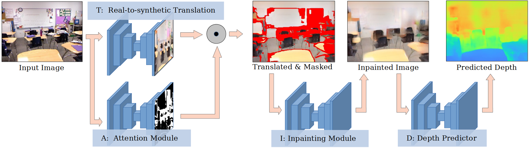
Figure 2: Flowchart of our whole ARC model in predicting the depth given a real-world image. The ARC framework performs real-to-synthetic translation of an input image to account for low-level domain shift and simultaneously detects the “hard” out-of-domain regions using a trained attention module $\cal A$. These regions are removed by multiplicative gating with the binary mask from $\cal A$ and the masked regions inpainted by module $\cal I$. The translated result is fed to final depth predictor module $\cal D$ which is trained to estimate depth from a mix of synthetic and (translated) real data.

3 Attend, Remove, Complete (ARC)

Recent methods largely focus on how to leverage synthetic data (and their annotations) along with real-world images (where no annotations are available) to train a model that performs well on real images later [24, 58]. We consider a more relaxed (and we believe realistic) scenario in which there is a small amount of real-world ground-truth data available during training. More formally, given a set of real-world labeled data $X^{r}=\{{\bf x}^{r}_{i},{\bf y}^{r}_{i}\}_{i=1}^{M}$ and a large amount of synthetic data $X^{s}=\{{\bf x}^{s}_{j},{\bf y}^{s}_{j}\}_{j=1}^{N}$, where $M\ll N$, we would like to train a monocular depth predictor $\cal D$, that accurately estimates per-pixel depth on real-world test images. The challenges of this problem are two-fold. First, due to the synthetic-real domain gap, it is not clear when including synthetic training data improves the test-time performance of a depth predictor on real images. Second, assuming the model does indeed benefit from synthetic training data, it is an open question as to how to best leverage the knowledge of domain difference between real and synthetic.

Our experiments positively answer the first question: synthetic data can be indeed exploited for learning better depth models, but in a non-trivial way as shown later through experiments. Briefly, real-world images contain complex regions (e.g., rare objects), which do not appear in the synthetic data. Such complex regions may negatively affect depth prediction by a model trained over large amounts of synthetic, clean images. Figure 2 demonstrates the inference flowchart of ARC, which learns to attend, remove and complete challenging regions in real-world test images in order to better match the low- and high-level domain statistics of synthetic training data. In this section, we elaborate each component module, and finally present the training pipeline.

3.1 Attention Module $\cal A$

How might we automatically discover the existence and appearance of “hard regions” that negatively affect depth learning and prediction? Such regions are not just those which are rare in the real images, but also include those which are common in real images but absent from our pool of synthetic training data. Finding such “hard regions” thus relies on both the depth predictor itself and synthetic data distribution. To discover this complex dependence, we utilize an attention module $\cal A$ that learns to automatically detect such “hard regions” from the real-world input images. Given a real image ${\bf x}^{r}\in{\mathbb{R}}^{H\times W\times 3}$ as input, the attention module produces a binary mask ${\bf M}\in{\mathbb{R}}^{H\times W}$ used for erasing the “hard regions” using simple Hadamard product ${\bf M}\odot{\bf x}^{r}$ to produce the resulting masked image.

One challenge is that producing a binary mask typically involves a hard-thresholding operation which is non-differentiable and prevents from end-to-end training using backpropagation. To solve this, we turn to the Gumbel-Max trick [21] that produces quasi binary masks using a continuous relaxation [26, 36].

We briefly summarize the “Gumbel max trick” [26, 36, 52]. A random variable $g$ follows a Gumbel distribution if $g=-\log(-\log(u))$, where $u$ follows a uniform distribution $U(0,1)$. Let $m$ be a discrete binary random variable with probability $P(m=1)\propto\alpha$, and let $g$ be a Gumbel random variable. Then, a sample of $m$ can be obtained by sampling $g$ from the Gumbel distribution and computing:

$${m}=\text{sigmoid}((\log(\alpha)+g)/\tau),$$ (1)

where the temperature $\tau\rightarrow 0$ drives the ${m}$ to take on binary values and approximates the non-differentiable argmax operation. We use this operation to generate a binary mask of size ${\bf M}\in{\mathbb{R}}^{H\times W}$.

To control the sparsity of the output mask ${\bf M}$, we penalize the empirical sparsity of the mask $\xi=\frac{1}{H*W}\sum_{i,j}^{H,W}{\bf M}_{i,j}$ using a KL divergence loss term [29]:

$$\ell_{KL}=\rho\log(\frac{\rho}{\xi})+(1-\rho)\log(\frac{1-\rho}{1-\xi}).$$ (2)

where hyperparameter $\rho$ controls the sparsity level (portion of pixels to keep). We apply the above loss term $\ell_{KL}$ in training our whole system, forcing the attention module $\cal A$ to identify the hard regions in an “intelligent” manner to target a given level of sparsity while still remaining the fidelity of depth predictions on the translated image. We find that training in conjunction with the other modules results in attention masks that tend to remove regions instead of isolated pixels (see Fig. 5)

3.2 Inpainting Module $\cal I$

The previous attention module $\cal A$ removes hard regions in ${\bf x}^{r}$ with sparse, binary mask ${\bf M}$, inducing holes in the image with the operation ${\bf M}\odot{\bf x}^{r}$. To avoid disrupting depth prediction we would like to fill in some reasonable values (without changing unmasked pixels). To this end, we adopt an inpainting module $\cal I$ that learns to fill in holes by leveraging knowledge from synthetic data distribution as well as the depth prediction loss. Mathematically we have:

$$\tilde{{\bf x}}=(1-{\bf M})\odot{\cal I}({\bf M}\odot{\bf x}^{r})+{\bf M}\odot{\bf x}^{r}.$$ (3)

To train the inpainting module $\cal I$, we pretrain with a self-supervised method by learning to reconstruct randomly removed regions using the reconstruction loss $\ell_{rec}^{rgb}$:

$$\ell_{rec}^{rgb}=\mathbb{E}_{x^{r}\sim X^{r}}[||{\cal I}({\bf M}\odot{\bf x}^{r})-{\bf x}^{r}||_{1}]$$ (4)

As demonstrated in [40], $\ell_{rec}^{rgb}$ encourages the model to learn remove objects instead of reconstructing the original images since removed regions are random. Additionally, we use two perceptual losses [55]. The first penalizes feature reconstruction:

$$\ell^{f}_{rec}=\sum\limits_{k=1}^{K}\mathbb{E}_{{\bf x}^{r}\sim X^{r}}[||\phi_{k}({\cal I}({\bf M}\odot{\bf x}^{r}))-\phi_{k}({\bf x}^{r})||_{1}],$$ (5)

where $\phi_{k}(\cdot)$ is the output feature at the $k^{th}$ layer of a VGG16 pretrained model [42]. The second perceptual loss is a style reconstruction loss that penalizes the differences in colors, textures, and common patterns.

$$\ell_{style}=\sum\limits_{k=1}^{K}\mathbb{E}_{x^{r}\sim X^{r}}[||\sigma^{\phi}_{k}({\cal I}({\bf M}\odot{\bf x}^{r}))-\sigma^{\phi}_{k}({\bf x}^{r})||_{1}],$$ (6)

where function $\sigma^{\phi}_{k}(\cdot)$ returns a Gram matrix. For the feature $\phi_{k}({\bf x})$ of size $C_{k}\times H_{k}\times W_{k}$, the corresponding Gram matrix $\sigma^{\phi}_{k}({\bf x}^{r})\in{\mathbb{R}}^{C_{k}\times C_{k}}$ is computed as:

$$\sigma^{\phi}_{k}({\bf x}^{r})=\frac{1}{C_{k}H_{k}W_{k}}R(\phi_{k}({\bf x}^{r}))\cdot R(\phi_{k}({\bf x}^{r}))^{T},$$ (7)

where $R(\cdot)$ reshapes the feature $\phi_{k}({\bf x})$ into $C_{k}\times H_{k}\ W_{k}$.

Lastly, we incorporate an adversarial loss $\ell_{adv}$ to force the inpainting module $\cal I$ to fill in pixel values that follow the synthetic data distribution:

$$\ell_{adv}=\mathbb{E}_{x^{r}\sim X^{r}}[\log(D(\tilde{{\bf x}}))]+\mathbb{E}_{{\bf x}^{s}\sim X^{s}}[\log(1-D({\bf x}^{s})],$$ (8)

where $D$ is a discriminator with learnable weights that is trained on the fly. To summarize, we use the following loss function to train our inpainting module $\cal I$:

$$\ell_{inp}=\ell_{rec}^{rgb}+\lambda_{f}\cdot\ell^{f}_{rec}+\lambda_{style}\cdot\ell_{style}+\lambda_{adv}\cdot\ell_{adv},$$ (9)

where we set weight parameters as $\lambda_{f}=1.0$, $\lambda_{style}=1.0$, and $\lambda_{adv}=0.01$ in our paper.

3.3 Style Translator Module $\cal T$

The style translator module $\cal T$ is the final piece to translate the real images into the synthetic data domain. As the style translator adapts low-level feature (e.g., color and texture) we apply it prior to inpainting. Following the literature, we train the style translator in a standard CycleGAN [60] pipeline, by minimizing the following loss:

$$\begin{split}\ell_{cycle}&=\mathbb{E}_{x^{r}\sim X^{r}}[||G_{s2r}(G_{r2s}(x^{r}))-x^{r}||_{1}]\\ &+\mathbb{E}_{x^{s}\sim X^{s}}[||G_{r2s}(G_{s2r}(x^{s}))-x^{s}||_{1}],\end{split}$$ (10)

where $\cal T$ = $G_{r2s}$ is the translator from direction real to synthetic domain; while $G_{s2r}$ is the other way around. Note that we need two adversarial losses $\ell^{r}_{adv}$ and $\ell^{s}_{adv}$ in the form of Eqn.(8) along with the cycle constraint loss $\ell_{cycle}$. We further exploit the identity mapping constraint to encourage translators to preserve the geometric content and color composition between original and translated images:

$$\begin{split}\ell_{id}&=\mathbb{E}_{x^{r}\sim X^{r}}[||G_{s2r}(x^{r})-x^{r}||_{1}]\\ &+\mathbb{E}_{x^{s}\sim X^{s}}[||G_{r2s}(x^{s})-x^{s}||_{1}].\end{split}$$ (11)

To summarize, the overall objective function for training the style translator $\cal T$ is:

$$\ell_{trans}=\lambda_{cycle}\cdot\ell_{cycle}+\lambda_{id}\cdot\ell_{id}+(\ell^{r}_{adv}+\ell^{s}_{adv}),$$ (12)

where we set the weights $\lambda_{cycle}=10.0$, $\lambda_{id}=5.0$.

3.4 Depth Predictor $\cal D$

We train our depth predictor $\cal D$ over the combined set of translated real training images $\tilde{{\bf x}}^{r}$ and synthetic images ${\bf x}^{s}$ using a simple $L_{1}$ norm based loss:

$$\begin{split}\ell_{d}=&\mathbb{E}_{({\bf x}^{r},{\bf y}^{r})\sim X^{r}}||{\cal D}(\tilde{{\bf x}}^{r})-y^{r}||_{1}\\ &+\mathbb{E}_{({\bf x}^{s},{\bf y}^{s})\sim X^{s}}||{\cal D}({\bf x}^{s})-{\bf y}^{s}||_{1}.\end{split}$$ (13)

3.5 Training by Modular Coordinate Descent

In principle, one might combine all the loss terms to train the ARC modules jointly. However, we found such practice difficult due to several reasons: bad local minima, mode collapse within the whole system, large memory consumption, etc. Instead, we present our proposed training pipeline that trains each module individually, followed by a fine-tuning step over the whole system. We note such a modular coordinate descent training protocol has been exploited in prior work, such as block coordinate descent methods [37, 1], layer pretraining in deep models [23, 42], stage-wise training of big complex systems [4, 7] and those with modular design [3, 11].

Concretely, we train the depth predictor module $\cal D$ by feeding the original images from either the synthetic set, or the real set or the mix of the two as a pretraining stage. For the synthetic-real style translator module $\cal T$, we first train it with CycleGAN. Then we insert the attention module $\cal A$ and the depth predictor module $\cal D$ into this CycleGAN, but fixing $\cal D$ and $\cal T$, and train the attention module $\cal A$ only. Note that after training the attention module $\cal A$, we fix it without updating it any more and switch the Gumbel transform to output real binary maps, on the assumption that it has already learned what to attend and remove with the help of depth loss and synthetic distribution. We train the inpainting module $\cal I$ over translated real-world images and synthetic images.

The above procedure yields good initialization for all the modules, after which we may keep optimizing them one by one while fixing the others. In practice, simply fine-tune the whole model (still fixing $\cal A$) with the depth loss term only, by removing all the adversarial losses. To do this, we alternate between minimizing the following two losses:

$$\begin{split}\ell^{1}_{d}&=\mathbb{E}_{({\bf x}^{r},{\bf y}^{r})\sim X^{r}}||{\cal D}({\cal I}({\cal T}({\bf x}^{r})\odot{\cal A}({\bf x}_{r}))))-{\bf y}^{r}||_{1}\\ &+\mathbb{E}_{({\bf x}^{s},{\bf y}^{s})\sim X^{s}}||{\cal D}({\bf x}^{s})-{\bf y}^{s}||_{1},\end{split}$$ (14)

$$\ell^{2}_{d}=\mathbb{E}_{({\bf x}^{r},{\bf y}^{r})\sim X^{r}}||{\cal D}({\cal I}({\cal T}({\bf x}^{r})\odot{\cal A}({\bf x}_{r}))))-{\bf y}^{r}||_{1}.$$ (15)

We find in practice that such fine-tuning better exploits synthetic data to avoid overfitting on the translated real images, and also avoids catastrophic forgetting [12, 28] on the real images in face of overwhelmingly large amounts of synthetic data.

4 Experiments

We carry out extensive experiments to validate our ARC model in leveraging synthetic data for depth prediction. We provide systematic ablation study to understand the contribution of each module and the sparsity of the attention module $\cal A$. We further visualize the intermediate results produced by ARC modules, along with failure cases, to better understand the whole ARC model and the high-level domain gap.

Table 1: A list of metrics used for evaluation in experiments, with their calculations, denoting by $y$ and $y^{*}$ the predicted and ground-truth depth in the validation set.

Abs Relative diff. (Rel)		$\frac{1}{|T|}\sum_{y\in T}|y-y^{*}|/y^{*}$
Squared Relative diff. (Sq-Rel)		$\frac{1}{|T|}\sum_{y\in T}||y-y^{*}||^{2}/y^{*}$
RMS		$\sqrt{\frac{1}{|T|}\sum_{y\in T}||y_{i}-y_{i}^{*}||^{2}}$
RMS-log		$\sqrt{\frac{1}{|T|}\sum_{y\in T}||\log y_{i}-\log y_{i}^{*}||^{2}}$
Threshold $\delta^{i}$,   $i$$\in$$\{1,2,3\}$		% of $y_{i}$ s.t. $\max(\frac{y_{i}}{y_{i}^{*}},\frac{y_{i}^{*}}{y_{i}})$$<$$1.25^{i}$

4.1 Implementation Details

Network Architecture. Every single module in our ARC framework is implemented by a simple encoder-decoder architecture as used in  [60], which also defines our discriminator’s architecture. We modify the decoder to output a single channel to train our attention module $\cal A$. As for the depth prediction module, we further add skip connections that help output high-resolution depth estimate [58].

Training. We first train each module individually for 50 epochs using the Adam optimizer [27], with initial learning rate 5$e$-5 (1$e$-4 for discriminator if adopted) and coefficients 0.9 and 0.999 for computing running averages of gradient and its square. Then we fine-tune the whole ARC model with the proposed modular coordinate descent scheme with the same learning parameters.

Datasets. We evaluate on indoor scene and outdoor scene datasets. For indoor scene depth prediction, we use the real-world NYUv2 [41] and synthetic Physically-based Rendering (PBRS) [56] datasets. NYUv2 contains video frames captured using Microsoft Kinect, with 1,449 test frames and a large set of video (training) frames. From the video frames, we randomly sample 500 as our small amount of labeled real data (no overlap with the official testing set). PBRS contains large-scale synthetic images generated using the Mitsuba renderer and SUNCG CAD models [43]. We randomly sample 5,000 synthetic images for training. For outdoor scene depth prediction, we turn to the Kitti [17] and virtual Kitti (vKitti) [14] datasets. In Kitti, we use the Eigen testing set to evaluate [59, 19] and the first 1,000 frames as the small amount of real-world labeled data for training [10]. With vKitti, we use the split $\{$clone, 15-deg-left, 15-deg-right, 30-deg-left, 30-deg-right$\}$ to form our synthetic training set consisting of 10,630 frames. Consistent with previous work, we clip the maximum depth in vKitti to 80.0m for training, and report performance on Kitti by capping at 80.0m for a fair comparison.

Comparisons and Baselines. We compare four classes of models. Firstly we have three baselines that train a single depth predictor on only synthetic data, only real data, or the combined set. Secondly we train state-of-the-art domain adaptation methods (T²Net [58], CrDoCo [6] and GASDA [57]) with their released code. During training, we also modify them to use the small amount of annotated real-world data in addition to the large-scale synthetic data. We note that these methods originally perform unsupervised domain adaptation, but they perform much worse than our modified baselines which leverage some real-world training data. This supports our suspicion that multiple losses involved in these methods (e.g., adversarial loss terms) do not necessarily contribute to reducing the depth loss. Thirdly, we have our ARC model and ablated variants to evaluate how each module helps improve depth learning. The fourth group includes a few top-performing fully-supervised methods which were trained specifically for the dataset over annotated real images only, but at a much larger scale For example, DORN [13] trains over more than 120K/20K frames for NYUv2/Kitti, respectively. This is 200/40 times larger than the labeled real images for training our ARC model.

Evaluation metrics. for depth prediction are standard and widely adopted in literature, as summarized in Table 1,

4.2 Indoor Scene Depth with NYUv2 & PBRS

Table 2: Quantitative comparison over NYUv2 testing set [41]. We train the state-of-the-art domain adaptation methods with the small amount of annotated real data in addition to the large-scale synthetic data. We design three baselines that only train a single depth predictor directly over synthetic or real images. Besides report full ARC model, we ablate each module or their combinations. We set $\rho$=0.85 in the attention module $\cal A$ if any, with more ablation study in Fig. 3. Finally, as reference, we also list a few top-performing methods that have been trained over several orders more annotated real-world frames.

Model/metric	$\downarrow$ lower is better				$\uparrow$ better
	Rel	Sq-Rel	RMS	RMS-log	$\delta^{1}$	$\delta^{2}$	$\delta^{3}$
State-of-the-art domain adaptation methods (w/ real labeled data)
T2Net [58]	0.202	0.192	0.723	0.254	0.696	0.911	0.975
CrDoCo [6]	0.222	0.213	0.798	0.271	0.667	0.903	0.974
GASDA [57]	0.219	0.220	0.801	0.269	0.661	0.902	0.974
Our (baseline) models.
syn only	0.299	0.408	1.077	0.371	0.508	0.798	0.925
real only	0.222	0.240	0.810	0.284	0.640	0.885	0.967
mix training	0.200	0.194	0.722	0.257	0.698	0.911	0.975
ARC: $\cal T$	0.226	0.218	0.805	0.275	0.636	0.892	0.974
ARC:$\cal A$	0.204	0.208	0.762	0.268	0.681	0.901	0.971
ARC: $\cal A$&$\cal T$	0.189	0.181	0.726	0.255	0.702	0.913	0.976
ARC: $\cal A$&$\cal I$	0.195	0.191	0.731	0.259	0.698	0.909	0.974
ARC: full	0.186	0.175	0.710	0.250	0.712	0.917	0.977
Training over large-scale NYUv2 video sequences ($>$120K)
DORN [13]	0.115	–	0.509	0.051	0.828	0.965	0.992
Laina [31]	0.127	–	0.573	0.055	0.811	0.953	0.988
Eigen [9]	0.158	0.121	0.641	0.214	0.769	0.950	0.988

Table 2 lists detailed comparison for indoor scene depth prediction. We observe that ARC outperforms other unsupervised domain adaptation methods by a substantial margin. This demonstrates two aspects. First, these domain adaptation methods have adversarial losses that force translation between domains to be more realistic, but there is no guarantee that “more realistic” is beneficial for depth learning. Second, removing “hard” regions in real images makes the real-to-synthetic translation easier and more effective for leveraging synthetic data in terms of depth learning. The second point will be further verified through qualitative results. We also provide an ablation study adding in the attention module $\mathcal{A}$ leads to better performance than merely adding the synthetic-real style translator $\mathcal{T}$. This shows the improvement brought by $\cal A$. However, combining $\cal A$ with either $\cal T$ or $\cal I$ improves further, while $\cal A$ & $\cal T$ is better as removing the hard real regions more closely matches the synthetic training data.

4.3 Outdoor Scene Depth with Kitti & vKitti

We train the same set of domain adaptation methods and baselines on the outdoor data, and report detailed comparisons in Table 3. We observe similar trends as reported in the indoor scenario in Table 2. Specifically, $\cal A$ is shown to be effective in terms of better performance prediction; while combined with other modules (e.g., $\cal T$ and $\cal I$) it achieves even better performance. By including all the modules, our ARC model (the full version) outperforms by a clear margin the other domain adaptation methods and the baselines. However, the performance gain here is not as remarkable as that in the indoor scenario. We conjecture this is due to several reasons: 1) depth annotation by LiDAR are very sparse while vKitti have annotations everywhere; 2) the Kitti and vKitti images are far less diverse than indoor scenes (e.g., similar perspective structure with vanishing point around the image center).

Table 3: Quantitative comparison over Kitti testing set [17]. The methods we compare are the same as described in Table 2, including three baselines, our ARC model and ablation studies, the state-of-the-art domain adaptation methods trained on both synthetic and real-world annotated data, as well as some top-performing methods on this dataset, which have been trained over three orders more annotated real-world frames from kitti videos.

Model/metric	$\downarrow$ lower is better				$\uparrow$ better
	Rel	Sq-Rel	RMS	RMS-log	$\delta^{1}$	$\delta^{2}$	$\delta^{3}$
State-of-the-art domain adaptation methods (w/ real labeled data)
T2Net [58]	0.151	0.993	4.693	0.253	0.791	0.914	0.966
CrDoCo [6]	0.275	2.083	5.908	0.347	0.635	0.839	0.930
GASDA [57]	0.253	1.802	5.337	0.339	0.647	0.852	0.951
Our (baseline) models.
syn only	0.291	3.264	7.556	0.436	0.525	0.760	0.881
real only	0.155	1.050	4.685	0.250	0.798	0.922	0.968
mix training	0.152	0.988	4.751	0.257	0.784	0.918	0.966
ARC: $\cal T$	0.156	1.018	5.130	0.279	0.757	0.903	0.959
ARC: $\cal A$	0.154	0.998	5.141	0.278	0.761	0.908	0.962
ARC: $\cal A$&$\cal T$	0.147	0.947	4.864	0.259	0.784	0.916	0.966
ARC: $\cal A$&$\cal I$	0.152	0.995	5.054	0.271	0.766	0.908	0.962
ARC: full	0.143	0.927	4.679	0.246	0.798	0.922	0.968
Training over large-scale kitti video frames ($>$20K)
DORN [13]	0.071	0.268	2.271	0.116	0.936	0.985	0.995
DVSO [53]	0.097	0.734	4.442	0.187	0.888	0.958	0.980
Guo [22]	0.096	0.641	4.095	0.168	0.892	0.967	0.986

4.4 Ablation Study and Qualitative Visualization

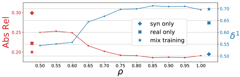
Figure 3: Ablation study of the sparsity factor $\rho$ of the ARC model on NYUv2 dataset. We use “Abs-Rel” and “or $\delta^{1}$” to measure the performance (see Table 1 for their definition). Note that the sparsity level $\rho$ cannot be exact 1.0 due to KL loss during training, so we present an approximate value with $\rho=0.99999$.

Table 4: Quantitative comparison between ARC and mix training baseline inside and outside of the mask region on NYUv2 testing set [41], where $\Delta$ represents the performance gain of ARC over mix training baseline under each metric.

Model/metric	$\downarrow$ lower is better				$\uparrow$ better
	Rel	Sq-Rel	RMS	RMS-log	$\delta^{1}$	$\delta^{2}$	$\delta^{3}$
Inside the mask (e.g., removed/inpainted)
mix training	0.221	0.259	0.870	0.282	0.661	0.889	0.966
ARC: full	0.206	0.232	0.851	0.273	0.675	0.895	0.970
$\Delta$	$\downarrow$0.015	$\downarrow$0.027	$\downarrow$0.019	$\downarrow$0.009	$\uparrow$0.014	$\uparrow$0.006	$\uparrow$0.004
Outside the mask
mix training	0.198	0.191	0.715	0.256	0.700	0.913	0.976
ARC: full	0.185	0.173	0.703	0.249	0.713	0.918	0.977
$\Delta$	$\downarrow$0.013	$\downarrow$0.018	$\downarrow$0.012	$\downarrow$0.007	$\uparrow$0.013	$\uparrow$0.005	$\uparrow$0.001

Figure 4: Sorted per-sample error reduction of ARC over the mix training baseline on NYUv2 dataset w.r.t the RMS-log metric. The error reduction is computed as RMS-log(ARC) $-$ RMS-log(mix training). The blue vertical line represents the index separating negative and positive error reduction.

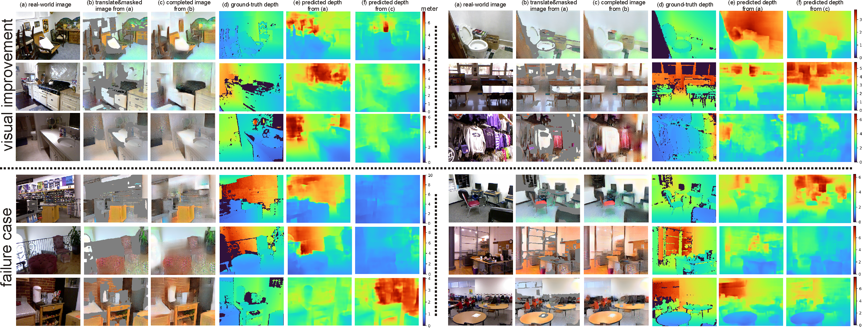
Figure 5: Qualitative results list some images over which our ARC model improves the depth prediction remarkably, as well as failure cases. (Best viewed in color and zoomed in.) More visualizations of ARC on Kitti and NYUv2 dataset are shown in the Appendices.

Sparsity level $\rho$ controls the percentage of pixels to remove in the binary attention map. We are interested in studying how the hyperparameter $\rho$ affects the overall depth prediction. We plot in Fig. 3 the performance vs. varied $\rho$ on two metrics (Abs-Rel and $\delta^{1}$). We can see that the overall depth prediction degenerates slowly with smaller $\rho$ at first; then drastically degrades when $\rho$ decreases to 0.8, meaning $\sim 20\%$ pixels are removed for a given image. We also depict our three baselines, showing that over a wide range of $\rho$. Note that ARC has slightly worse performance when $\rho=1.0$ (strictly speaking, $\rho=0.99999$) compared to $\rho=0.95$. This observation shows that remove a certain amount of pixels indeed helps depth predictions. The same analyses on Kitti dataset are shown in the Appendices.

Per-sample improvement study to understand where our ARC model performs better over a strong baseline. We sort and plot the per-image error reduction of ARC over the mix training baseline on NYUv2 testing set according to the RMS-log metric, shown in Fig. 4. The error reduction is computed as RMS-log(ARC) $-$ RMS-log(mix training). It’s easy to observe that ARC reduces the error for around 70% of the entire dataset. More importantly, ARC decreases the error over 0.2 at most when the average error of ARC and our mix training baseline are 0.252 and 0.257, respectively.

Masked regions study analyzes how ARC differs from mix training baseline on “hard” pixels and regular pixels. For each sample in the NYUv2 testing set, we independently compute the depth prediction performance inside and outside of the attention mask. As shown in Table 4, ARC improves the depth prediction not only inside but also outside of the mask regions on average. This observation suggests that ARC improves the depth prediction globally without sacrificing the performance outside of the mask.

Qualitative results are shown in Fig. 5, including some random failure cases (measured by performance drop when using ARC). These images are from NYUv2 dataset. Kitti images and their results can be found in the Appendices. From the good examples, we can see ARC indeed removes some cluttered regions that are intuitively challenging: replacing clutter with simplified contents, e.g., preserving boundaries and replacing bright windows with wall colors. From an uncertainty perspective, removed pixels are places where models are less confident. By comparing with the depth estimate over the original image, ARC’s learning strategy of “learn to admit what you don’t know” is superior to making confident but often catastrophically poor predictions. It is also interesting to analyze the failure cases. For example, while ARC successfully removes and inpaints rare items like the frames and cluttered books in the shelf, it suffers from over-smooth areas that provide little cues to infer the scene structure. This suggests future research directions, e.g. improving modules with the unsupervised real-world images, inserting a high-level understanding of the scene with partial labels (e.g. easy or sparse annotations) for tasks in which real annotations are expensive or even impossible (e.g., intrinsics).

5 Conclusion

We present the ARC framework which learns to attend, remove and complete “hard regions” that depth predictors find not only challenging but detrimental to overall depth prediction performance. ARC learns to carry out completion over these removed regions in order to simplify them and bring them closer to the distribution of the synthetic domain. This real-to-synthetic translation ultimately makes better use of synthetic data in producing an accurate depth estimate. With our proposed modular coordinate descent training protocol, we train our ARC system and demonstrate its effectiveness through extensive experiments: ARC outperforms other state-of-the-art methods in depth prediction, with a limited amount of annotated training data and a large amount of synthetic data. We believe our ARC framework is also applicable of boosting performance on a broad range of other pixel-level prediction tasks, such as surface normals and intrinsic image decomposition, where per-pixel annotations are similarly expensive to collect. Moreover, ARC hints the benefit of uncertainty estimation that requires special attention to the “hard” regions for better prediction.

Acknowledgements This research was supported by NSF grants IIS-1813785, IIS-1618806, a research gift from Qualcomm, and a hardware donation from NVIDIA.

References

- [1] Michal Aharon, Michael Elad, and Alfred Bruckstein. K-svd: An algorithm for designing overcomplete dictionaries for sparse representation. IEEE Transactions on signal processing, 54(11):4311–4322, 2006.
- [2] Peter Anderson, Xiaodong He, Chris Buehler, Damien Teney, Mark Johnson, Stephen Gould, and Lei Zhang. Bottom-up and top-down attention for image captioning and visual question answering. In Proceedings of the IEEE Conference on Computer Vision and Pattern Recognition, pages 6077–6086, 2018.
- [3] Jacob Andreas, Marcus Rohrbach, Trevor Darrell, and Dan Klein. Neural module networks. In Proceedings of the IEEE Conference on Computer Vision and Pattern Recognition, pages 39–48, 2016.
- [4] Elnaz Barshan and Paul Fieguth. Stage-wise training: An improved feature learning strategy for deep models. In Feature Extraction: Modern Questions and Challenges, pages 49–59, 2015.
- [5] Daniel J Butler, Jonas Wulff, Garrett B Stanley, and Michael J Black. A naturalistic open source movie for optical flow evaluation. In European conference on computer vision, pages 611–625. Springer, 2012.
- [6] Yun-Chun Chen, Yen-Yu Lin, Ming-Hsuan Yang, and Jia-Bin Huang. Crdoco: Pixel-level domain transfer with cross-domain consistency. In Proceedings of the IEEE Conference on Computer Vision and Pattern Recognition, pages 1791–1800, 2019.
- [7] Zaiyi Chen, Zhuoning Yuan, Jinfeng Yi, Bowen Zhou, Enhong Chen, and Tianbao Yang. Universal stagewise learning for non-convex problems with convergence on averaged solutions. arXiv preprint arXiv:1808.06296, 2018.
- [8] Alexey Dosovitskiy, Philipp Fischer, Eddy Ilg, Philip Hausser, Caner Hazirbas, Vladimir Golkov, Patrick Van Der Smagt, Daniel Cremers, and Thomas Brox. Flownet: Learning optical flow with convolutional networks. In Proceedings of the IEEE international conference on computer vision, pages 2758–2766, 2015.
- [9] David Eigen and Rob Fergus. Predicting depth, surface normals and semantic labels with a common multi-scale convolutional architecture. In Proceedings of the IEEE international conference on computer vision, pages 2650–2658, 2015.
- [10] David Eigen, Christian Puhrsch, and Rob Fergus. Depth map prediction from a single image using a multi-scale deep network. In Advances in neural information processing systems, pages 2366–2374, 2014.
- [11] Zhiyuan Fang, Shu Kong, Charless Fowlkes, and Yezhou Yang. Modularized textual grounding for counterfactual resilience. In Proceedings of the IEEE Conference on Computer Vision and Pattern Recognition, pages 6378–6388, 2019.
- [12] Robert M French. Catastrophic forgetting in connectionist networks. Trends in cognitive sciences, 3(4):128–135, 1999.
- [13] Huan Fu, Mingming Gong, Chaohui Wang, Kayhan Batmanghelich, and Dacheng Tao. Deep ordinal regression network for monocular depth estimation. In Proceedings of the IEEE Conference on Computer Vision and Pattern Recognition, pages 2002–2011, 2018.
- [14] Adrien Gaidon, Qiao Wang, Yohann Cabon, and Eleonora Vig. Virtual worlds as proxy for multi-object tracking analysis. In Proceedings of the IEEE conference on computer vision and pattern recognition, pages 4340–4349, 2016.
- [15] Yaroslav Ganin and Victor Lempitsky. Unsupervised domain adaptation by backpropagation. arXiv preprint arXiv:1409.7495, 2014.
- [16] Jonas Gehring, Michael Auli, David Grangier, Denis Yarats, and Yann N Dauphin. Convolutional sequence to sequence learning. In Proceedings of the 34th International Conference on Machine Learning-Volume 70, pages 1243–1252. JMLR. org, 2017.
- [17] Andreas Geiger, Philip Lenz, Christoph Stiller, and Raquel Urtasun. Vision meets robotics: The kitti dataset. The International Journal of Robotics Research, 32(11):1231–1237, 2013.
- [18] Golnaz Ghiasi, Tsung-Yi Lin, and Quoc V Le. Dropblock: A regularization method for convolutional networks. In Advances in Neural Information Processing Systems, pages 10727–10737, 2018.
- [19] Clément Godard, Oisin Mac Aodha, Michael Firman, and Gabriel J Brostow. Digging into self-supervised monocular depth estimation. In Proceedings of the IEEE International Conference on Computer Vision, pages 3828–3838, 2019.
- [20] Ian Goodfellow, Jean Pouget-Abadie, Mehdi Mirza, Bing Xu, David Warde-Farley, Sherjil Ozair, Aaron Courville, and Yoshua Bengio. Generative adversarial nets. In Advances in neural information processing systems, pages 2672–2680, 2014.
- [21] Emil Julius Gumbel. Statistics of extremes. Courier Corporation, 2012.
- [22] Xiaoyang Guo, Hongsheng Li, Shuai Yi, Jimmy Ren, and Xiaogang Wang. Learning monocular depth by distilling cross-domain stereo networks. In ECCV, 2018.
- [23] Geoffrey E Hinton and Ruslan R Salakhutdinov. Reducing the dimensionality of data with neural networks. science, 313(5786):504–507, 2006.
- [24] Judy Hoffman, Eric Tzeng, Taesung Park, Jun-Yan Zhu, Phillip Isola, Kate Saenko, Alexei A Efros, and Trevor Darrell. Cycada: Cycle-consistent adversarial domain adaptation. arXiv preprint arXiv:1711.03213, 2017.
- [25] Phillip Isola, Jun-Yan Zhu, Tinghui Zhou, and Alexei A Efros. Image-to-image translation with conditional adversarial networks. In Proceedings of the IEEE conference on computer vision and pattern recognition, pages 1125–1134, 2017.
- [26] Eric Jang, Shixiang Gu, and Ben Poole. Categorical reparameterization with gumbel-softmax. In International Conference on Learning Representations (ICLR), 2017.
- [27] Diederik P Kingma and Jimmy Ba. Adam: A method for stochastic optimization. arXiv preprint arXiv:1412.6980, 2014.
- [28] James Kirkpatrick, Razvan Pascanu, Neil Rabinowitz, Joel Veness, Guillaume Desjardins, Andrei A Rusu, Kieran Milan, John Quan, Tiago Ramalho, Agnieszka Grabska-Barwinska, et al. Overcoming catastrophic forgetting in neural networks. Proceedings of the national academy of sciences, 114(13):3521–3526, 2017.
- [29] Shu Kong and Charless Fowlkes. Pixel-wise attentional gating for scene parsing. In 2019 IEEE Winter Conference on Applications of Computer Vision (WACV), pages 1024–1033. IEEE, 2019.
- [30] Philipp Krähenbühl. Free supervision from video games. In Proceedings of the IEEE Conference on Computer Vision and Pattern Recognition, pages 2955–2964, 2018.
- [31] Iro Laina, Christian Rupprecht, Vasileios Belagiannis, Federico Tombari, and Nassir Navab. Deeper depth prediction with fully convolutional residual networks. In 2016 Fourth international conference on 3D vision (3DV), pages 239–248. IEEE, 2016.
- [32] Colin Levy and Ton Roosendaal. Sintel. In ACM SIGGRAPH ASIA 2010 Computer Animation Festival, page 82. ACM, 2010.
- [33] Zhengqi Li and Noah Snavely. Cgintrinsics: Better intrinsic image decomposition through physically-based rendering. In Proceedings of the European Conference on Computer Vision (ECCV), pages 371–387, 2018.
- [34] Mingsheng Long, Yue Cao, Jianmin Wang, and Michael I Jordan. Learning transferable features with deep adaptation networks. arXiv preprint arXiv:1502.02791, 2015.
- [35] Mingsheng Long, Guiguang Ding, Jianmin Wang, Jiaguang Sun, Yuchen Guo, and Philip S Yu. Transfer sparse coding for robust image representation. In Proceedings of the IEEE conference on computer vision and pattern recognition, pages 407–414, 2013.
- [36] Chris J Maddison, Andriy Mnih, and Yee Whye Teh. The concrete distribution: A continuous relaxation of discrete random variables. arXiv preprint arXiv:1611.00712, 2016.
- [37] Julien Mairal, Francis Bach, Jean Ponce, and Guillermo Sapiro. Online dictionary learning for sparse coding. In Proceedings of the 26th annual international conference on machine learning, pages 689–696. ACM, 2009.
- [38] Phuc Nguyen, Ting Liu, Gautam Prasad, and Bohyung Han. Weakly supervised action localization by sparse temporal pooling network. In Proceedings of the IEEE Conference on Computer Vision and Pattern Recognition, pages 6752–6761, 2018.
- [39] Sinno Jialin Pan and Qiang Yang. A survey on transfer learning. IEEE Transactions on knowledge and data engineering, 22(10):1345–1359, 2009.
- [40] Rakshith R Shetty, Mario Fritz, and Bernt Schiele. Adversarial scene editing: Automatic object removal from weak supervision. In Advances in Neural Information Processing Systems, pages 7706–7716, 2018.
- [41] Nathan Silberman, Derek Hoiem, Pushmeet Kohli, and Rob Fergus. Indoor segmentation and support inference from rgbd images. In European Conference on Computer Vision, pages 746–760. Springer, 2012.
- [42] Karen Simonyan and Andrew Zisserman. Very deep convolutional networks for large-scale image recognition. arXiv preprint arXiv:1409.1556, 2014.
- [43] Shuran Song, Fisher Yu, Andy Zeng, Angel X Chang, Manolis Savva, and Thomas Funkhouser. Semantic scene completion from a single depth image. Proceedings of 30th IEEE Conference on Computer Vision and Pattern Recognition, 2017.
- [44] Baochen Sun and Kate Saenko. Deep coral: Correlation alignment for deep domain adaptation. In European Conference on Computer Vision, pages 443–450. Springer, 2016.
- [45] Yaoru Sun and Robert Fisher. Object-based visual attention for computer vision. Artificial intelligence, 146(1):77–123, 2003.
- [46] Yi-Hsuan Tsai, Wei-Chih Hung, Samuel Schulter, Kihyuk Sohn, Ming-Hsuan Yang, and Manmohan Chandraker. Learning to adapt structured output space for semantic segmentation. In Proceedings of the IEEE Conference on Computer Vision and Pattern Recognition, pages 7472–7481, 2018.
- [47] Eric Tzeng, Judy Hoffman, Trevor Darrell, and Kate Saenko. Simultaneous deep transfer across domains and tasks. In Proceedings of the IEEE International Conference on Computer Vision, pages 4068–4076, 2015.
- [48] Eric Tzeng, Judy Hoffman, Kate Saenko, and Trevor Darrell. Adversarial discriminative domain adaptation. In Proceedings of the IEEE Conference on Computer Vision and Pattern Recognition, pages 7167–7176, 2017.
- [49] Eric Tzeng, Judy Hoffman, Ning Zhang, Kate Saenko, and Trevor Darrell. Deep domain confusion: Maximizing for domain invariance. arXiv preprint arXiv:1412.3474, 2014.
- [50] Gul Varol, Javier Romero, Xavier Martin, Naureen Mahmood, Michael J Black, Ivan Laptev, and Cordelia Schmid. Learning from synthetic humans. In Proceedings of the IEEE Conference on Computer Vision and Pattern Recognition, pages 109–117, 2017.
- [51] Ashish Vaswani, Noam Shazeer, Niki Parmar, Jakob Uszkoreit, Llion Jones, Aidan N Gomez, Łukasz Kaiser, and Illia Polosukhin. Attention is all you need. In Advances in neural information processing systems, pages 5998–6008, 2017.
- [52] Andreas Veit and Serge Belongie. Convolutional networks with adaptive inference graphs. In Proceedings of the European Conference on Computer Vision (ECCV), pages 3–18, 2018.
- [53] Nan Yang, Rui Wang, Jörg Stückler, and Daniel Cremers. Deep virtual stereo odometry: Leveraging deep depth prediction for monocular direct sparse odometry. In ECCV, 2018.
- [54] Amir R Zamir, Alexander Sax, William Shen, Leonidas J Guibas, Jitendra Malik, and Silvio Savarese. Taskonomy: Disentangling task transfer learning. In Proceedings of the IEEE Conference on Computer Vision and Pattern Recognition, pages 3712–3722, 2018.
- [55] Richard Zhang, Phillip Isola, Alexei A Efros, Eli Shechtman, and Oliver Wang. The unreasonable effectiveness of deep features as a perceptual metric. In Proceedings of the IEEE Conference on Computer Vision and Pattern Recognition, pages 586–595, 2018.
- [56] Yinda Zhang, Shuran Song, Ersin Yumer, Manolis Savva, Joon-Young Lee, Hailin Jin, and Thomas Funkhouser. Physically-based rendering for indoor scene understanding using convolutional neural networks. The IEEE Conference on Computer Vision and Pattern Recognition (CVPR), 2017.
- [57] Shanshan Zhao, Huan Fu, Mingming Gong, and Dacheng Tao. Geometry-aware symmetric domain adaptation for monocular depth estimation. In Proceedings of the IEEE Conference on Computer Vision and Pattern Recognition, pages 9788–9798, 2019.
- [58] Chuanxia Zheng, Tat-Jen Cham, and Jianfei Cai. T2net: Synthetic-to-realistic translation for solving single-image depth estimation tasks. In Proceedings of the European Conference on Computer Vision (ECCV), pages 767–783, 2018.
- [59] Tinghui Zhou, Matthew Brown, Noah Snavely, and David G Lowe. Unsupervised learning of depth and ego-motion from video. In Proceedings of the IEEE Conference on Computer Vision and Pattern Recognition, pages 1851–1858, 2017.
- [60] Jun-Yan Zhu, Taesung Park, Phillip Isola, and Alexei A Efros. Unpaired image-to-image translation using cycle-consistent adversarial networks. In Proceedings of the IEEE international conference on computer vision, pages 2223–2232, 2017.
- [61] Jun-Yan Zhu, Richard Zhang, Deepak Pathak, Trevor Darrell, Alexei A Efros, Oliver Wang, and Eli Shechtman. Toward multimodal image-to-image translation. In Advances in Neural Information Processing Systems, pages 465–476, 2017.