Fast moving pulsars as probes of interstellar medium

Abstract

Pulsars moving through ism produce bow shocks detected in hydrogen H$\alpha$ line emission. The morphology of the bow shock nebulae allows one to probe the properties of ism on scales $\sim 0.01$ pc and smaller. We performed 2D rmhd modeling of the pulsar bow shock and simulated the corresponding H$\alpha$ emission morphology. We find that even a mild spatial inhomogeneity of ism density, $\delta\rho/\rho\sim 1$, leads to significant variations of the shape of the shock seen in H$\alpha$ line emission. We successfully reproduce the morphology of the Guitar Nebula. We infer quasi-periodic density variations in the warm component of ism with characteristic length of $\sim 0.1$ pc. Structures of this scale might be also responsible for the formation of the fine features seen at the forward shock of Tycho snr in X-rays. Formation of such short periodic density structures in the warm component of ism is puzzling, and bow-shock nebulae provide unique probes to study this phenomenon.

1 Introduction

Pulsars produce ultra-relativistic winds that create Pulsar Wind Nebulae (PWNe,pwn Rees & Gunn, 1974; Gaensler & Slane, 2006; Kargaltsev & Pavlov, 2008; Kargaltsev et al., 2015; Reynolds et al., 2017). Many fast moving pulsars quickly escape the host supernova remnant (for a recent review see Kargaltsev et al., 2017a). The proper speed of such pulsars vary in a wide range from a few kilometers per second to more than a thousand kilometers per second. Typically, these velocities are much larger than the sound speeds in the ism, $c_{s,}{}_{\textsc{ism}}\sim 10-100\,\mathrm{km\,s^{-1}}$.

The interaction of a fast moving pulsar wind with the ism produces a bow-shock nebula with extended tail. The X-ray emission of the bow-shock was discussed by Barkov et al. (2019a); Olmi & Bucciantini (2019); the filamentary structure created by non-thermal particles escaping from PWN was researched by Bandiera (2008); Barkov & Lyutikov (2019); Barkov et al. (2019b).

In the apex part of the pwn the ism ram pressure confines the pulsar wind producing two shocks – forward shock in the ism and the reverse/ts in the pulsar wind; the two shock are separated by the contact discontinuity (CD). This picture is similar to the structure formed by interaction of the Solar wind with the Local ism (see Zank, 1999; Pogorelov et al., 2017, for review).

Early works on the structure of the bow shock nebulae (e.g. Bucciantini et al., 2005) predicted a smooth morphology. In contrast, the observations show large morphological variations (Kargaltsev et al., 2017b), both of the pwn part (regions encompassing the shocked pulsar wind) and the shape of the bow shock (in the ism part of the interaction region). Especially puzzling is the Guitar Nebula, which shows what can be called “closed in the back” morphology: shocks, delineated by the $H\alpha$ emission, bend/curve towards the tail, not the head part.

Variations of the pwn part of the interacting flow are likely due to the internal dynamics of the shocked pulsar wind: mass loading (Morlino et al., 2015; Olmi et al., 2018), as well as fluid and current-driven instabilities (Barkov et al., 2019a) can induce larger variations in the shape of the confined pulsar wind. (We note here that so far no simulations were able to catch the long term dynamics in the tails, on scales much longer than the stand-off distances.)

One of the goals of the present study is to investigate whether the variations of the pwn part of the flow can affect the shape of the forward shock (e.g., as discussed by van Kerkwijk & Ingle, 2008). Our simulations indicate that the internal dynamics of the pwn part does not affect the bow shock in any appreciable way. The basic reason is that the mildly relativistic flow within the pwn tail quickly advects downstream all the perturbations, see §4.

We then resort to external perturbations to produce the morphological variations of the $H\alpha$ emission maps. We target the Guitar Nebula as the extreme example of a nontrivial morphology of the forward shock. The most surprising morphological feature of the Guitar Nebula is a sequence of “closed in the back” shocks (Vigelius et al., 2007; Yoon & Heinz, 2017; Toropina et al., 2019). Several fast moving pulsars form nebulae with $H\alpha$ line emission (Brownsberger & Romani, 2014), which show sequences of “closed in the back” shocks similar to those seen in the Guitar Nebula. As we demonstrate, the “closed in the back” morphology is a result of the projection effect (due to particular combination of the line of sight) and of the physical properties of the system (pulsar’s velocity and ism density variations).

2 Physics of hydrogen ionisation

A fast moving pulsar form a bow shock that heats the electrons and ions from ism. Hot electrons ionize neutral atoms and thermalize with them. The pressure balance between the pulsar wind and the ism gives the stand-off distance $r_{s}$

$$r_{s}=\sqrt{\frac{L{}_{\textsc{w}}}{4\uppi c\rho{}_{\textsc{ism}}\varv{}_{\textsc{ns}}^{2}}}=4\times 10^{16}L{}_{\textsc{w,\tiny\,36}}^{1/2}\,n{}_{\textsc{ism,\tiny\,0}}^{-1/2}\varv{}_{\textsc{ns,\tiny\,7.5}}^{-1}\,{\rm cm}\,,$$ (1)

where $L{}_{\textsc{w}}$ is pulsar spin-down luminosity, $\varv{}_{\textsc{ns}}$ is the velocity of pulsar, $\rho{}_{\textsc{ism}}=\mu m_{p}n{}_{\textsc{ism}}$ is ism mass and number density (here $m_{p}$ is mass of proton, $\mu=1.4$ is chemical composition factor). We use the following normalization agreement: $A=10^{x}A_{x}\rm\,cgs\,units$. The pass-though time, which is the characteristic time for crossing the stand-off distance, is

$$t_{s}=r_{s}/\varv{}_{\textsc{ns}}=1.3\times 10^{9}L{}_{\textsc{w,\tiny\,36}}^{1/2}\,n{}_{\textsc{ism,\tiny\,0}}^{-1/2}\varv{}_{\textsc{ns,\tiny\,7.5}}^{-2}\,{\rm s}\,.$$ (2)

Let us next estimate the ionization and recombination rates for hydrogen at the shock front. Following the work (Rossi et al., 1997) the ionization rate is

$$\frac{\foreach\x in{x{}_{\scriptscriptstyle HI}}{\mathrm{d}\hskip 0.80002pt\x\,}}{\foreach\x in{t}{\mathrm{d}\hskip 0.80002pt\x\,}}=n_{e}\left[c_{r}(1-x{}_{\scriptscriptstyle HI})-c_{i}x{}_{\scriptscriptstyle HI}\right]$$ (3)

here $n_{e}=n{}_{\scriptscriptstyle H}\left[(1-x{}_{\scriptscriptstyle HI})+0.001\right]$ is electron concentration, $c_{i}$ and $c_{r}$ are ionization and recombination rate coefficients

$$c_{i}=5.8\times 10^{-11}\sqrt{T_{0}}\exp{\left(-\frac{1.57\times 10^{5}}{T_{0}}\right)}\quad\mathrm{cm^{3}\,s^{-1}}$$ (4)

and

$$c_{r}=2.6\times 10^{-11}\frac{1}{\sqrt{T_{0}}}\quad\mathrm{cm^{3}\,s^{-1}}.$$ (5)

In the case of a fast moving pulsar the temperature behind the bow shock can be as high as $T\simeq 2\times 10^{6}\varv{}_{\textsc{ns,\tiny\,7.5}}^{2}\rm\,K$. At such high temperatures ionization processes dominates over recombination ones by far ($c_{i}\approx 10^{-7}\varv{}_{\textsc{ns,\tiny\,7.5}}$ and $c_{r}\approx 2\times 10^{-14}\varv{}_{\textsc{ns,\tiny\,7.5}}^{-1}$ cm^-3 s^-1). The ionization time scale can be estimated as

$$t_{i}=\frac{1}{c_{i}n_{e}}\sim 10^{7}n_{e}^{-1}\varv{}_{\textsc{ns,\tiny\,7.5}}^{-1}\mbox{ s}.$$ (6)

Comparing Eq. (2) and Eq. (6) we can see $t_{i}\ll t_{s}$, it means that the ionization is very fast and thickness of the ionization shell should be small. In contrast, the recombination time scale $t_{r}\sim 5\times 10^{13}\varv{}_{\textsc{ns,\tiny\,7.5}}$ is much longer as compared to the pass-through time scale. Some atoms ionization process is accompanied by excitation and emission of $H\alpha$ line. The most efficient condition of $H\alpha$ line emission is near $x{}_{\scriptscriptstyle HI}\approx 0.5$. As the ionization proceeds in a significantly more compact region compare to recombination one, it should be responsible for generation of the most distinct line emission. Thus, H$\alpha$ emission is produced in a thin shell right behind the bow shock. Only for slow pulsars, with velocity below $10^{7}$ cm s^-1, the ionization shell thickness can be comparable with the bow shock size.

Using the algorithm suggested by Rossi et al. (1997), hydro-dynamical data as density, pressure and $x{}_{\scriptscriptstyle HI}$ (see section 3.1) allow us to calculate the excitation rate of hydrogen and intensity of H$\alpha$ line emission as

$$\dot{e}{}_{\scriptscriptstyle H\alpha}=n{}_{\scriptscriptstyle H}n_{e}x{}_{\scriptscriptstyle HI}j{}_{\scriptscriptstyle H\alpha}\qquad\mbox{$\mathrm{erg}$\,$\mathrm{cm^{3}\,s^{-1}}$}$$ (7)

and emissivity coefficient

$$j{}_{\scriptscriptstyle H\alpha}=\frac{\hbar^{2}\sqrt{2\uppi}}{k_{B}^{1/2}m_{e}^{3/2}}q_{12}\frac{h\nu{}_{\scriptscriptstyle H\alpha}}{1+\left(q_{21}/A_{21}\right)}\quad\mbox{$\mathrm{erg}$\, cm}^{-3}\mbox{ s}^{-1},$$ (8)

here

$$q_{21}=\frac{8.6\times 10^{-6}}{T_{0}^{1/2}}\frac{\Omega_{21}}{g_{2}}$$ (9)

and

$$q_{12}=\frac{8.6\times 10^{-6}}{T_{0}^{1/2}}\frac{\Omega_{12}}{g_{1}}\exp{\left(-\frac{h\nu{}_{\scriptscriptstyle H\alpha}}{k_{B}T}\right)},$$ (10)

where parameters $g_{1}$, $g_{2}$ and $\Omega_{21}=\Omega_{12}$ are tabulated in PLUTO code.

3 Method

We implement a two-step procedure to calculate the expected morphology of the H$\alpha$ emission. First, as described in §3.1 we perform relativistic mhd simulations of a pulsar moving through inhomogeneous ism. These calculations define the shape of the bow shock and values of all relevant hydrodynamic parameters. Next, §3.2, we performed post-processing of the hydrodynamic data to calculate H$\alpha$ emissivity maps.

3.1 Numerical Setup

We performed a number of 2d rmhd simulations of the interaction of relativistic pulsar wind with external medium. The simulations were performed using a 2d geometry in Cylindrical coordinates using the PLUTO code (Mignone et al., 2007). Spatial parabolic interpolation, a 2^nd order Runge-Kutta approximation in time, and an HLLC Riemann solver were used Mignone & Bodo (2005). PLUTO is a modular Godunov-type code entirely written in C and intended mainly for astrophysical applications and high Mach number flows in multiple spatial dimensions. The simulations were performed on CFCA XC50 cluster of national astronomical observatory of Japan (NAOJ). The flow has been approximated as an ideal, relativistic adiabatic gas, one particle species, and polytropic index of 4/3. The size of the domain is $R\in[0,20a]$, $Z\in[-3a,100a]$ where the length unit $a=10^{16}$ cm (the initial ism velocity is directed along $Z$-axis). To have a good resolution in the central region and long the tail zone we use a non-uniform resolution in the computational domain. For “high-resolution” simulations we adopted the following grid configuration. Number of the radial cells in a high resolution uniform grid in the central region (for $R\in[0,1a]$) is $N_{\rm R,in}=520$. The outer non-uniform grid (for region with $R\in[1a,20a]$) has $N_{\rm R,out}=1560$ radial cells. In the Z direction we also adopted a non-uniform grid with three different zones. The inlet part ($Z\in[-3a,-1a]$) has $N_{\rm Z,out-}=520$ non-uniform grid. The central part (for $Z\in[-1a,1a]$) has a uniform grid with $N_{\rm Z,in}=1040$ cells, and the non-uniform tail grid (for $Z\in[1a,100a]$) contains $N_{\rm Z,out+}=4680$ cells. The grid parameters in “low-resolution” models are the following: $N_{\rm R,in}=130$ and $N_{\rm R,out}=390$ for the radial direction; $N_{\rm Z,out-}=130$, $N_{\rm Z,in}=260$, and $N_{\rm Z,out+}=1170$ for the Z-direction. See Table 1 for other parameters.

We used a so called simplified non-equilibrium cooling (SNEq) block of PLUTO code (see details in Rossi et al., 1997). Which allows to calculate the fraction of neutral atoms of hydrogen $x{}_{\scriptscriptstyle HI}$ in ism taking into account ionization and recombination processes. Moreover, the radiation loses for 16 lines (like Ly $\alpha$, HeI (584+623), OII (3727) etc.) are included in the energy equation.

3.2 H$\alpha$ emissivity maps

To obtain H$\alpha$ brightness maps, Eq. (7) needs to be integrated over the line of sight. These calculation were performed at the postprocessing stage on a workstation-class PC. Despite the simplicity of the numerical procedure, obtaining of high-resolution synthetic maps required quite a large amount of computations. The character of required calculations, i.e. integration over the line of sight, implies a case for effective GPU computing. We utilized PyCUDA, a CUDA API implementation for python, which allowed us to profit python visualization library matplotlib and get access to high-performance GPU computations, which were performed on NVIDIA TITAN V card. The synthetic maps were obtained in Cartesian coordinate system, with Z-axis directed towards the observer. We adopted a uniform XY-grid with resolution of $1536\times 1024$, which is sufficient for the comparison with observations. The symmetry axis of the mhd cylindrical box is assumed to locate in the XZ-plane and to make angle $\theta$ with X-axis (“viewing angle”). The size of the mhd computational box determined the interval of integration over Z-axis. The transformation of the Cartesian coordinates to the cylindrical of the mhd box were performed with a recursive procedure that allowed some improvement of the algorithm performance. At the integration points the intensity of H$\alpha$ emission was computed by bilinear interpolation between the most nearby nodes of the $RZ$ array obtained with PLUTO simulations. As the dependence of the emission intensity along the line-of-sight is sectionally linear we used trapezoidal integration method. Some further details of the postprocessing script are given in Appendix A.

We simulate interaction of ns supersonically moving in the ism with varying density profile given by

$$n{}_{\textsc{ism}}(z,t)=\frac{n_{0}}{1-a_{\rho}\cos\left[\frac{(z-\varv{}_{\textsc{ns}}t)}{d{}_{\textsc{w}}}\right]},$$ (11)

here $n_{0}=1/$cm³ is ism concentration, $d{}_{\textsc{w}}=3\times 10^{17}$ cm wave length, $a_{\rho}$ is wave amplitude and $\varv{}_{\textsc{ns}}$ ns speed in ism, the values $\varv{}_{\textsc{ns}}$ and $a_{\rho}$ for the models can be found in the Tab. 1. In all cases we assume Mach number in the ism $M{}_{\textsc{ism}}=\varv{}_{\textsc{ns}}/c_{s,\,}{}_{\textsc{ism}}=30$.

We initiate the pulsar wind as spherically symmetric with Lorentz factor 4.9 which corresponds to initial Mach number 45. Anisotropy of the pulsar wind (Bogovalov & Khangoulyan, 2002) may have certain impact on the morphology of the pwn, but the forward shock is much less sensitive to the pulsar wind anisotropy (Barkov et al., 2019a). We adopt the spindown luminosity for fast and slow models which forms forward termination shock at the distance $r_{s}=10^{16}$ cm (see eq.1) if $n{}_{\textsc{ism}}=1/$cm³. This value corresponds to $L{}_{\textsc{w}}=5.6\times 10^{38}\,\mathrm{erg\,s^{-1}}$ for fast and $L{}_{\textsc{w}}=1.4\times 10^{36}\,\mathrm{erg\,s^{-1}}$ for slow models respectively.

4 Results

4.1 Overall PWN properties

Table 1: Models parameters. Here presented name of the models, resolution in radial “R” and axial “Z” directions, neutron star speed $\varv{}_{\textsc{ns}}$, density amplitude variation parameter $a_{\rho}$ and pulsar wind power $L{}_{\textsc{w}}$.

Name	R	Z	$\varv{}_{\textsc{ns}}/c$	$a_{\rho}$	$L{}_{\textsc{w,\tiny\,36}}$
hr-fast-const	2080	6240	0.1	0	560
hr-fast-var3	2080	6240	0.1	0.5	560
lr-fast-var3	520	1560	0.1	0.5	560
lr-SNEq-slow-var3	520	1560	0.005	0.5	1.4
lr-SNEq-slow-var2	520	1560	0.005	0.2	1.4

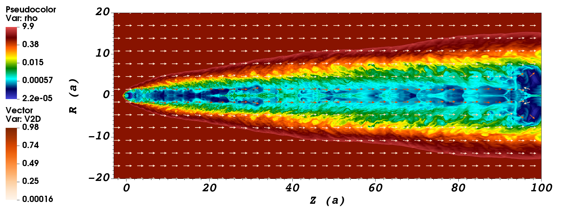
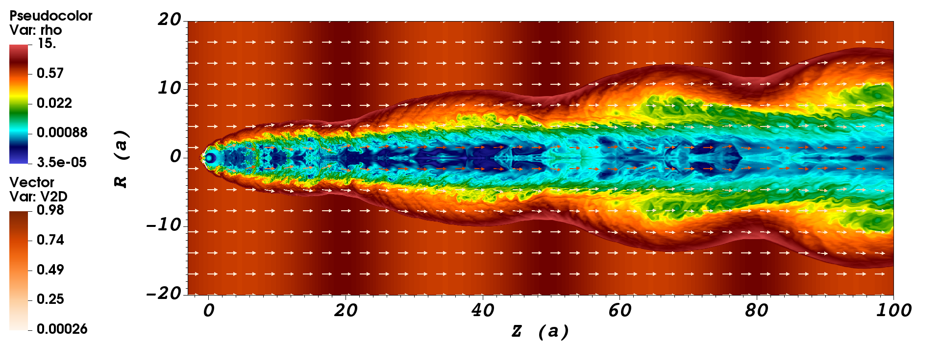
Figure 1: Color maps of density (log-scale) for hr-fast-const and hr-fast-var3 models (see Tab. 1 for detail) in the top and bottom panels, respectively. Arrows show the velocity field, the arrow color defines the flow speed (linear scale, speed of light units).

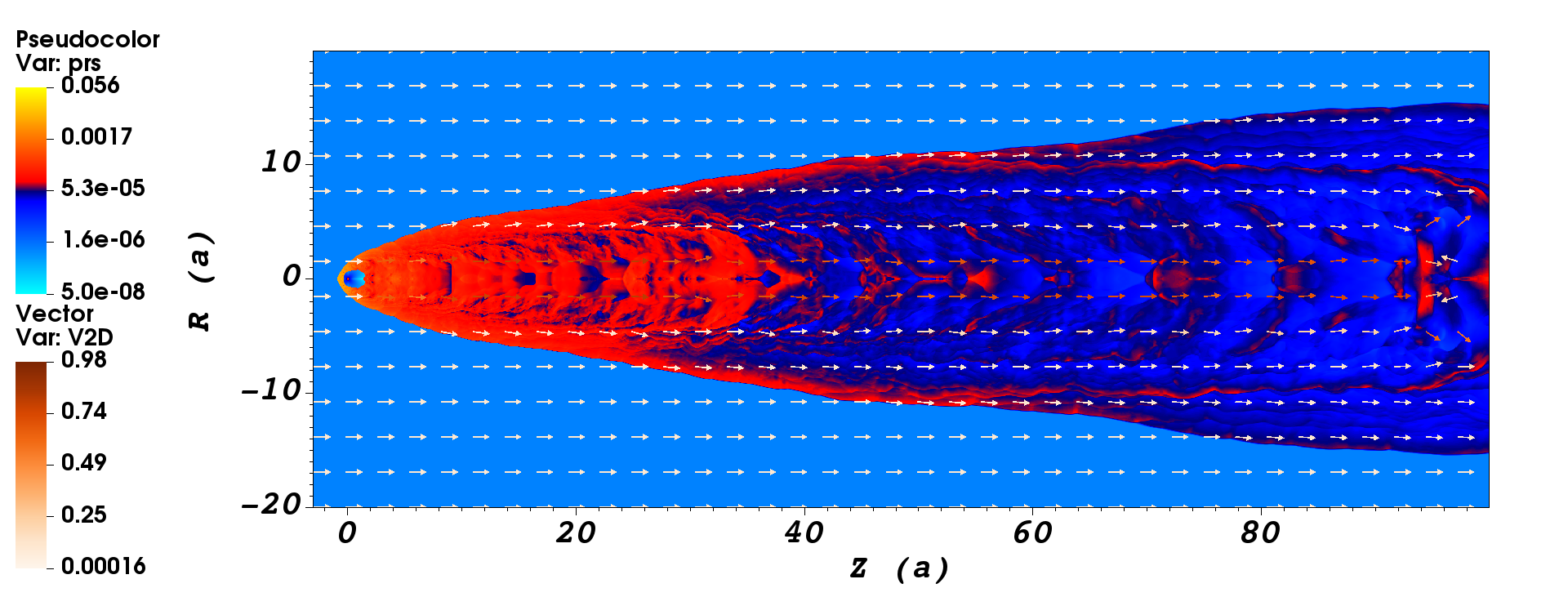
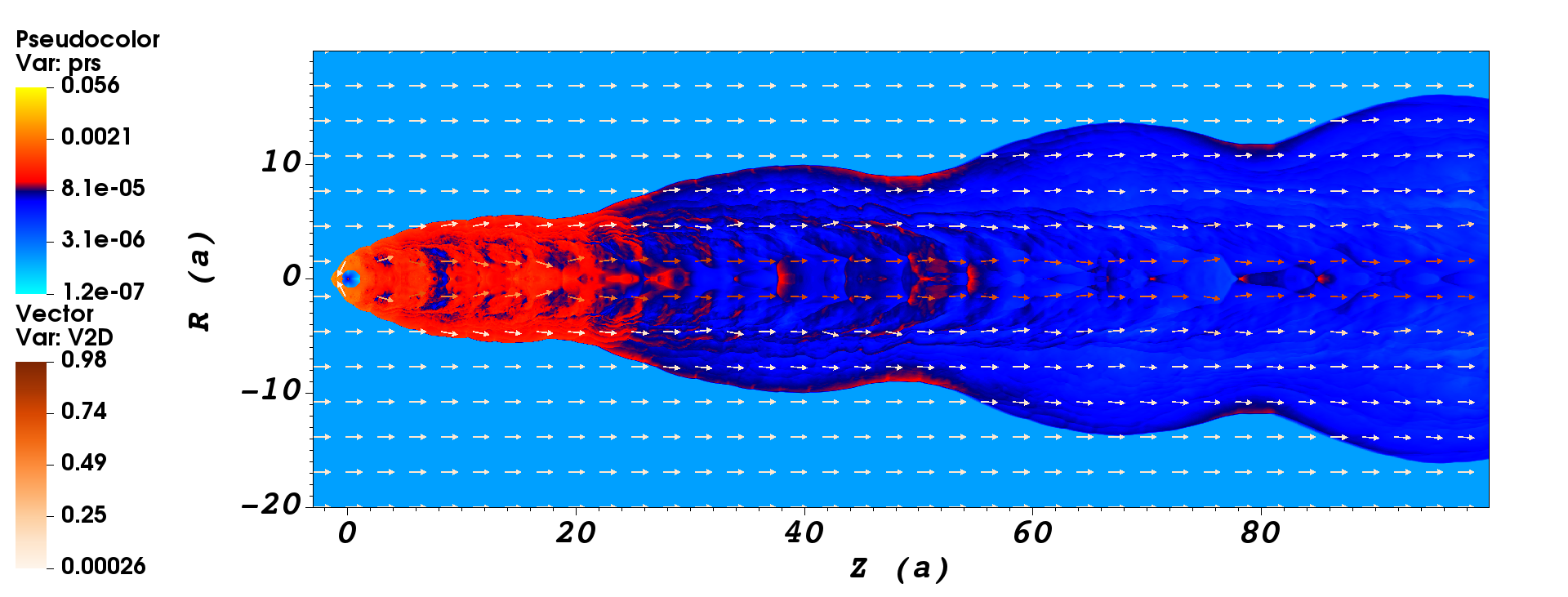
Figure 2: Color maps of pressure (log-scale) for hr-fast-const and hr-fast-var3 models (see Tab. 1 for detail) in the top and bottom panels, respectively. Arrows show the velocity field, the arrow color defines the flow speed (linear scale, speed of light units).

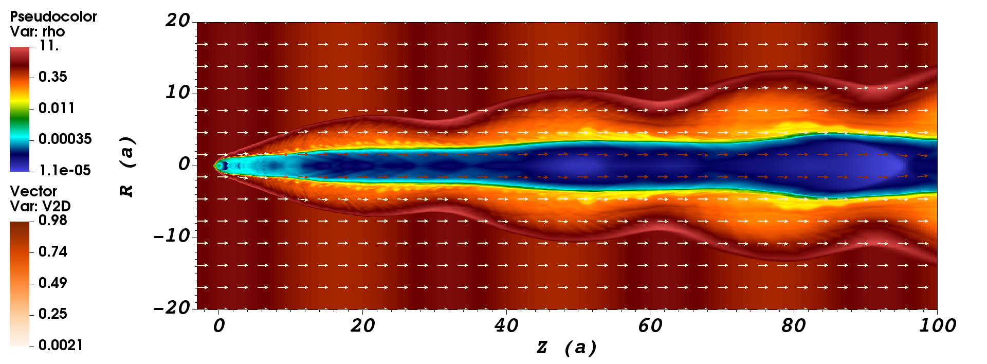
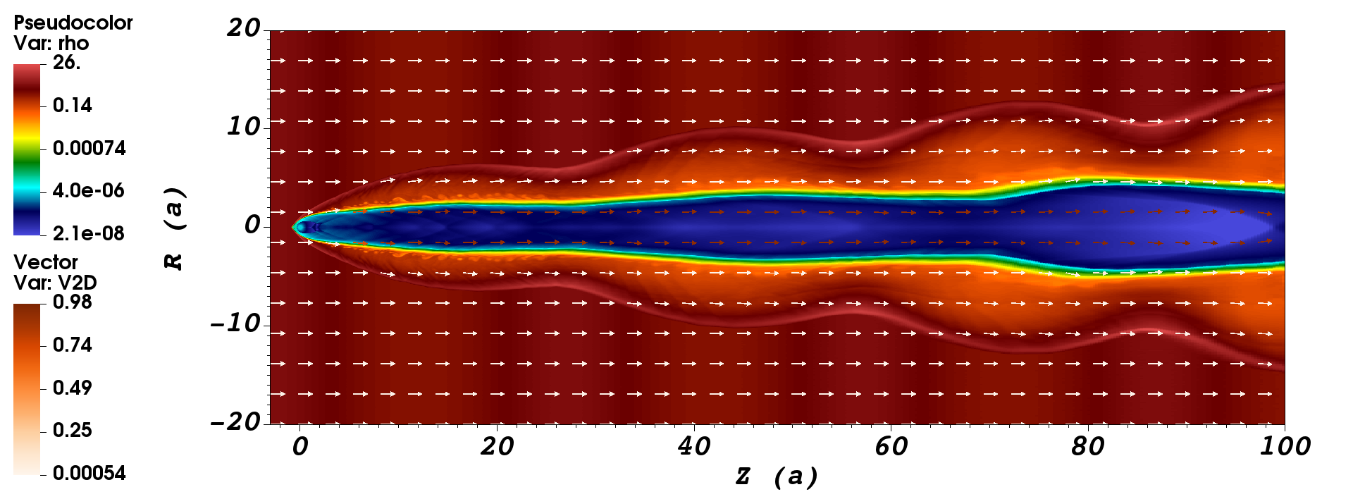
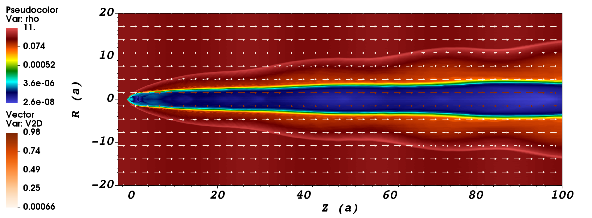
Figure 3: Color maps of density (log-scale) for three “low-resolution” models: lr-fast-var3 (top panel), lr-SNEq-slow-var3 (middle panel), and lr-SNEq-fast-var2 (which has a smaller variation of ism density, bottom panel). Arrows show the velocity field, the arrow color defines the flow speed (linear scale, speed of light units).

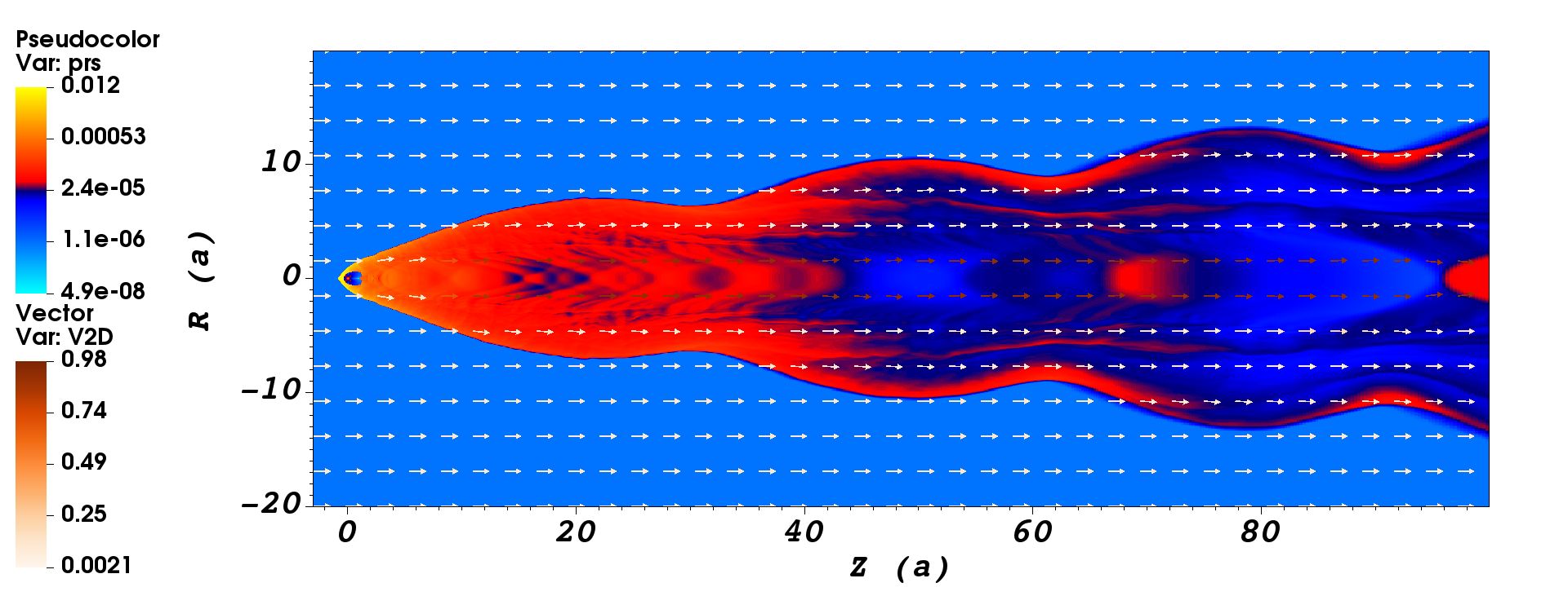
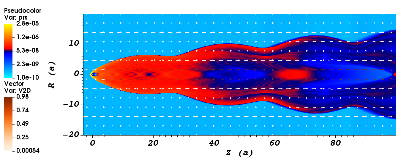
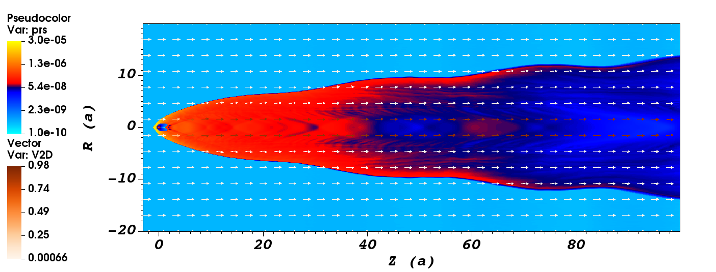
Figure 4: Color maps of pressure (log-scale) the same models as in Fig. 3. Arrows show the velocity field, the arrow color defines the flow speed (linear scale, speed of light units).

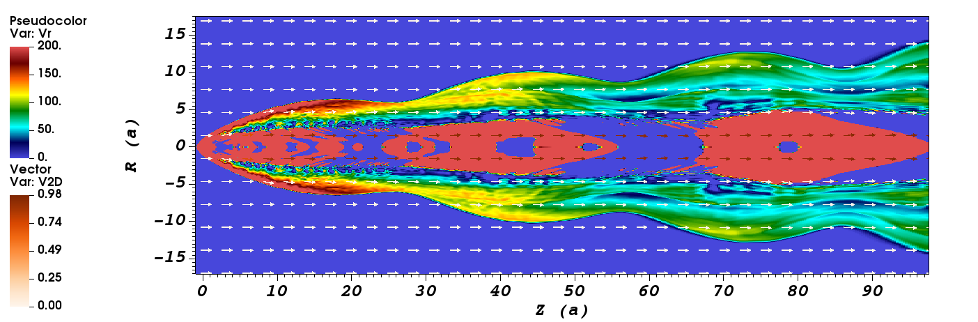
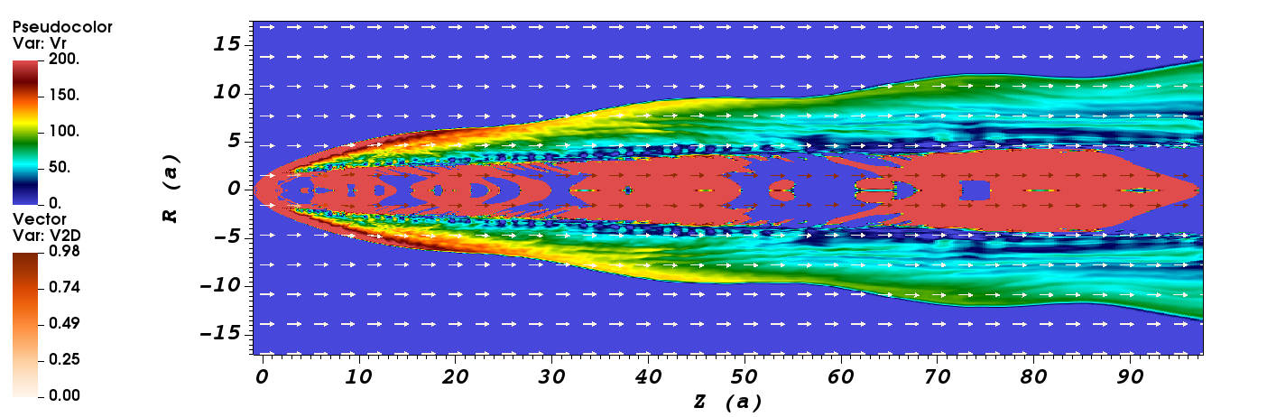
Figure 5: Color maps of radial velocity (linear-scale, [$\mathrm{km\,s^{-1}}$] units) for two “low-resolution” models with slower pulsar speed: lr-SNEq-slow-var3 (top panel), and lr-SNEq-slow-var2 (which has a smaller variation of ism density, bottom panel). Arrows show the velocity field, the arrow color defines the flow speed (linear scale, speed of light units).

Figure 6: $H\alpha$ line emission maps for model lr-SNEq-slow-var2. Viewing angle is 0.1 radian.

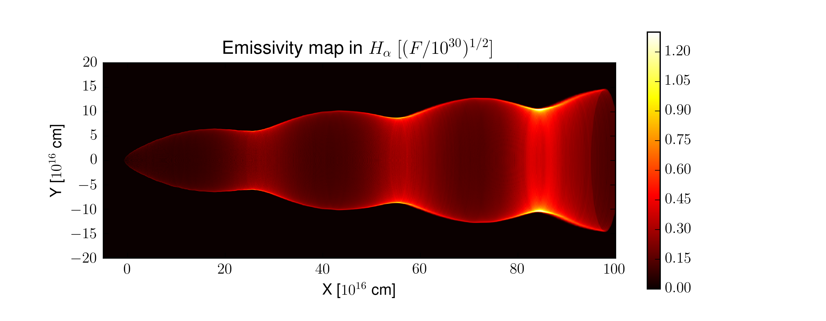
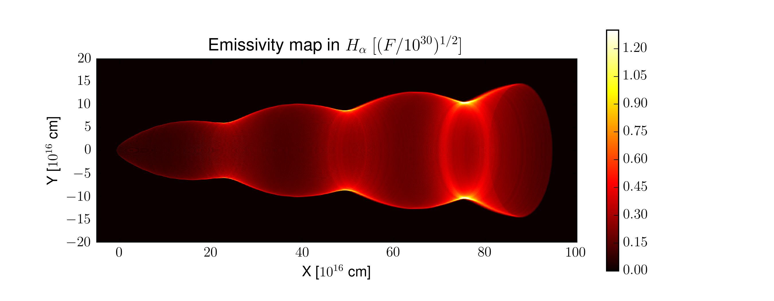
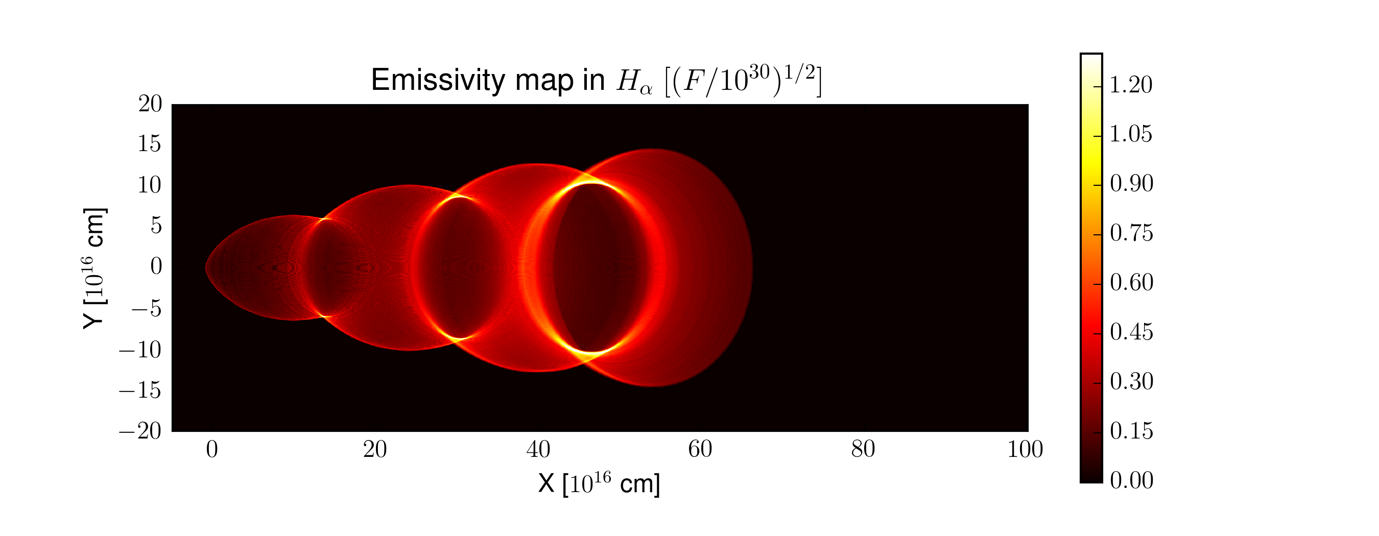
Figure 7: $H\alpha$ line emission maps for the model lr-SNEq-slow-var3 and three different viewing angles: 0.1 radian (top panel), 0.5 (middle panel), and 1 (bottom panel).

We performed five runs with different spacial resolutions and model parameters to illustrate how system evolves and which parameters play a crucial role. All the relevant parameters for each run are summarized in Table 1. We name each run accordingly the following simple rule: “run resolution (hr, lr or lr-SNEq)” – “pulsar velocity (fast or slow)” – “ism spatial dependence (const or var2 or var3)”. All the simulations were performed in the reference frame where the pulsar is at rest, and the ism is injected from the most left border of the computational domain (which corresponds to $z=-3a$). At the ism inlet the flow velocity was set to $\varv{}_{\textsc{ns}}$ and the density is determined by Eq. (11) for $z=-3a$.

In the model hr-fast-const we inject ism matter with constant density (i.e., $a_{\rho}=0$ in Eq. (11)) and velocity set to $0.1c$ (see Table 1). On top panels of Fig. 1 and Fig. 2 distributions of density and pressure are shown. In these figures one can see the expected flow structure: a pulsar surrounded by the unshocked pulsar wind; at larger radii a relativistic shock wave is formed; the shocked pulsar wind and ism matter are separated by a cd surface; a forward shock front takes place in the ism. On the right side from the pulsar, the shocks form a channel filled by material from the pulsar wind, which is surrounded by the shocked ism matter. The shock in the ism has a very smooth conical shape.

We see a significant growth of the kh instability at the cd between the shocked pulsar wind and ism. The kh instability triggers the formation of significant perturbations in the shocked pulsar wind region, so ism matter occasionally mixes with the shocked pulsar wind. These dense obstacles in the pulsar wind trigger the formation of additional shocks which potentially could deform the shape of the bow shock in ism. However, the large difference (a few orders of magnitude) between the sound speed in the shocked ism matter and the bulk speed of the shocked pulsar wind makes it almost impossible to develop a significant deformation of the shock front in ism. We can see the confirmation of described process in the upper panels of Fig. 1 and Fig. 2.

The quasistationary phase of simulation for the model hr-fast-var3 with periodic density distribution is presented in on the bottom panel of Fig. 1 and Fig. 2. Here we injected the ism matter with variable density ($a_{\rho}=0.5$ in Eq. (11)). A strong modulation of the shape of the ism shock can be seen. The shape of the cd is very complicated in this simulation. We can see a series of hierarchical structures which linked to the growth of small scale vertexes triggered by kh instability. On a larger scale, one can see elongated eddies triggered by the ism density variation. Interesting, the impact on the crossection of the shocked pulsar wind channel is significantly smaller compared to the variation of the crossection of forward shock in ism.

The gas pressure, shown in Fig. 2, for the model hr-fast-const indicates on a series of more-or-less uniformly distributed shocks which are triggered in the pulsar wind channel and propagate outside in the shocked material. The exact position of the cd is difficult to localize in this figure. The model hr-fast-var3 reveals a different behavior,: a series of shocks, which look like recollimation ones, can be localized just behind the high density front in the ism.

The models with slower ns velocity require a much longer computational time, so these models were computed with a smaller computational resolution. To verify eligibility of this resolution we also performed one simulation with this resolution for a faster moving ns.

First, let’s discuss the differences and similarities between the model lr-fast-var3 (Fig. 3) and hr-fast-var3 (Fig. 1). The shape of the forward shock in ism is essentially the same. The main difference is the structure of the cd surface, which in the case of lr-fast-var3 is much smoother if compared to the one obtained in hr-fast-var3 simulations. It can be explained by the influence of the numerical viscosity which suppresses the growth of the kh instability. The pressure maps (Fig. 4) show similarity of the bow shock shapes, also we see similar recollimation shocks. The high pressure zones in pulsar wind follows the high density zones in the ISM. The difference is the absence of fine structures in the shocked pulsar wind channel. In the low resolution case, the recollimation shocks have smoother structure. As we explained in § 2 and it is shown below, the optical lines are produced at the forward shock in the ism. The shocked pulsar wind zone is predominately filled with electron-positron pairs and should not produce any considerable amount of $H\alpha$ emission. We therefore safely claim that the resolution does not change significantly the geometry and properties of the $H\alpha$ emitting region.

The “slow” models feature a significantly larger density jump between the ism and the pulsar wind (see Fig. 3). The cd is more stable and the kh instability does not disrupt the pulsar wind channel. On the other hand, the forward shock shapes are almost identical in all *-var3 models. The pressure distributions are also very similar between lr-fast-var3 and lr-SNEq-slow-var3 models.

The amplitude of the density variation has a strong impact on the shape of the bow shock in ism (see Fig. 4). A variation of density by a factor of 3 (model lr-SNEq-slow-var3) creates a forward shock with a clear wavy shape, which is correlated to the ism density profile: the higher density, the smaller cylindrical radius of the shock. A model with a small density variation, lr-SNEq-slow-var2, still features a wavy-shaped bow shock. The recollimation shocks in the pulsar wind channel are visible and have a spatial lag relative to the density peaks in the ism.

In Fig. 5 we show the distribution of the radial component of speed in cylindrical coordinates for two models, lr-SNEq-slow-var3 and lr-SNEq-slow-var2. The radial speed at the shock decreases with the distance from the pulsar. On top of the decreasing trend, one can also see some speed increases in the low ism density regions. These increases are mostlikely related to the change of the sound speed in ism $c_{s}=\sqrt{\gamma_{g}p_{g}/\rho_{g}}$. In the case of the considered models, even for “slow” models, the pulsar moves with record speed as compared to pulsars found in Galaxy. The “sweet spot” speed for $H\alpha$ line production is about $10^{2}\,\mathrm{km\,s^{-1}}$. For such speed, the hydrogen ionization front is relatively thick, which makes the emission process to be efficient. In our simulations such speeds appear only on at the edge of the computational domain (see the right part of Fig. 5). As can be seen in Figs. 6 and  7 the $H\alpha$ line emission appears to be the most bright in this regime. In the case of a realistic ns proper speed, the bright $H\alpha$ region should appear close to the forward shock apex.

4.2 $H\alpha$ line intensity distribution

In Fig. 7 synthetic emissivity maps are shown for different viewing angles, $\theta=0.1$, $0.5$, and $1$ radian, from the top to the bottom. The high density peaks in ism are clearly visible as bright rings. Even a relatively small variation of the ism density leads to a very clear change of the surface brightens, with two important factors amplifying the emission: 1) total particle density; and 2) thickness of the ionization front. If the impact of the former factor is straightforward, ($I\propto n^{2}$), addressing the latter one is more complicated. If the shock is too fast, the ionization take place almost instantly and no neutral hydrogen left to emit after shock front. If shock is too slow, hydrogen atoms do not get excited and we again do not expect any significant line emission. Therefore, to see the $H\alpha$ nebula pulsar should move with velocity $\varv{}_{\textsc{ns,\tiny\,7.5}}\sim 1$.

The observational data (Brownsberger & Romani, 2014) show very similar features, the brighter are regions which seem to have the smaller radius, which should correspond to high ism density filaments crossed by the pulsar.

If ism density has a more complicated distribution (as we see in Brownsberger & Romani, 2014), one can expect a formation of structures which are more complex than ring-like structures revealed with our 2d simulations. For example, depending on the viewing angle even axial symmetric 2d distributions of emissivity can appear as bright triangles or lenses (see Fig. 7, bottom). We plan to further investigate the formation of complex structures in a future study with 3d mhd simulations.

4.3 Guitar Nebula

The parallax to pulsar B2224$+$65 measured with VLBI is $1.2^{+0.17}_{-0.2}$ mas (Deller et al., 2019), which corresponds to a distance of $D=830^{+170}_{-100}$ pc. The observations of Guitar Nebula (Chatterjee & Cordes, 2002; Dolch et al., 2016) in $H\alpha$ line revealed several depressions of the forward shock with the angular distance of $15^{\prime\prime}-30^{\prime\prime}$ between depression. This corresponds to a linear distance of $2-5\times 10^{17}$ cm (or $\sim 0.1$ pc). A comparison of the Guitar Nebula morphology with our synthetic emissivity maps (see Fig. 7) show that a modest modulation of the ism density, $\delta\rho/\rho\approx 0.8$, can result in such shape of the forward shock. The recent observations indicate that the pulsar a few years ago passed through a region with even higher density, $\delta\rho/\rho\sim 2$ (Dolch et al., 2016).

The pulsar producing the Guitar Nebula moves nearly in the plane of sky. We expect that for this configuration transverse density gradients will not produce distinct morphological features. In contrast, when the line of sight is nearly aligned with the pulsar’s velocity large morphological variations are expected (Brownsberger & Romani, 2014).

In the X-ray energy band, Chandra observations revealed a compact emitter spatially coinciding with pulsar B2224$+$65 and a filament structure extending by $\sim 2$ arcmin to the north-west (i.e., making angle of $\sim 118^{\circ}$ with the pulsar proper velocity) (Hui & Becker, 2007). The flux corresponding to the compact emitter is $\sim 1.8\times 10^{-14}\;\mathrm{erg\,s^{-1}\,cm^{-2}}$ (Johnson & Wang, 2010) and its extension is limited by $0.5^{\prime\prime}$ (Hui & Becker, 2007). For the source distance of 830 pc these parameters translates to $L_{\rm keV}=1.5\times 10^{30}\mathrm{erg\,s^{-1}}$ and $6\times 10^{15}\rm\,cm$. Because of its point-like nature, the compact emitter was associated with the pulsar. Similarly to pwn around isolated pulsar, bow-shock nebulae also feature extended non-thermal emission (Kargaltsev et al., 2017b). The characteristic size of X-ray morphology is comparable to the radius of the termination shock (Barkov et al., 2019a), i.e., $\sim 10^{16}\rm\,cm$ in the case of Guitar Nebula. In this region, adiabatic losses should dominate in the energy range responsible for the production of X-ray emission. According to Eq.(22) from Barkov et al. (2019a), X-ray luminosity of the extended nebula should be at the level of $0.1\%$ of the power responsible for acceleration of the keV-emitting electrons, i.e., fainter compare to the reported pulsar emission. We therefore conclude that Chandra observatory is not expected to detect the extended emission of Guitar Nebula.

The extended structure in Guitar Nebula can be associated with non-thermal particles escaping from pwn (Bandiera, 2008; Barkov et al., 2019b). For example, Bandiera (2008) argued that the X-ray feature reacquires ism magnetic field of $B\sim 50\rm\,\upmu G$. Large scale magnetic field can influence the shape of the termination shock. The magnetic field impact at the shock is determined by the gas normal velocity, $\varv_{s,n}$, and the Alfven speed, which is $\varv_{A}\sim 10^{7}\rm\,cm\,s^{-1}$ (for $B=50\rm\,\upmu G$ and plasma density of $\rho=1/\mbox{cm}^{3}$). The relative distortion of the forward shock can be estimated as $\left(\varv^{\prime}-\varv_{s,n}\right)/\varv_{s,n}$, where $\varv^{\prime}=\sqrt{\varv_{s,n}^{2}+\varv_{A}^{2}}$. For fast mowing pulsars, like B2224$+$65, the gas normal velocity is also very high, $\varv_{s,n}\sim\varv{}_{\textsc{ns}}\approx 10^{8}\rm\,cm\,s^{-1}$, thus the relative deformation of the forward shock remains small, $\sim 0.01$. We therefore conclude that the suggested scenario for the formation of $H_{\alpha}$ morphology in Guitar Nebula is consistent with the X-ray observations.

4.4 Connection to other observations

The Herschel satellite imaging observations of nearby molecular clouds (Miville-Deschênes et al., 2010), show that filamentary structures are characterized by length-scales with a relatively narrow distribution around a length of $\sim 0.1$ pc. This spreads within a factor of two for a wide range of column densities (Arzoumanian et al., 2011, 2019; Koch & Rosolowsky, 2015; Roy et al., 2019). These observations probe the cold component of ism, $T\sim 10\rm\,K$. The properties of the hot ($T\sim 10^{6}$ K) and warm ($T\sim 10^{4}$ K) components of ism are less known. As the hot and warm components are distributed in the interstellar space between the molecular clouds, their low densities make impossible obtaining of any meaningful constrains with CO line emission, as in the case of the molecular clouds. As shown above, $H\alpha$ emission from forward shocks created by fast moving pulsars is very sensitive to the density of ism, which allows one to obtain unique information about density structure of the warm ism. Our interpretation of the Guitar Nebula suggests that the warm component of ism features density filaments of the same length scale as cold ism as revealed with Hershel observations.

Interesting, the stripe structure seen in X-rays at the forward shock wave of snr Tycho has a similar length scale. The characteristic angular size of $l_{gap}\sim 8^{\prime\prime}$ corresponds to linear size $\sim 0.1$ pc (Decourchelle et al., 2001; Kosenko, 2006; Eriksen et al., 2011). Previously, these X-ray stripes were interpreted as a result of non-linear particle acceleration in turbulent media (Bykov et al., 2011; Caprioli & Spitkovsky, 2013). Based on similarity of the linear size of X-ray features seen in Tycho and density fluctuations inferred around the Guitar Nebula, we suggest that these structures, intrinsic to the upstream medium, are illuminated by the passage of the shock. Further down stream, strong turbulence (triggered, e.g. by the Relay-Taylor instability Warren et al., 2005) erases these structures.

Similar structures might have also been detected spectroscopically in the snrs RX J0852.0$\textendash$4622 and Vela (Pakhomov et al., 2012). Line profiles were indicating a presence of accelerating clouds, with sizes similar to the size of those inferred in the Guitar Nebula and Tycho snr, $\sim 0.1$ pc.

We also note that the structures we inferred in the warm ism around the Guitar Nebula should have different origin from the ones producing filaments in dense Galactic molecular clouds (e.g. Arzoumanian et al., 2011). In the case of molecular clouds the parsec-scale filaments correspond approximately to the Jeans length. The warm component of ISM has much higher temperature ($\sim 10^{4}$ K) and respectively much larger Jeans length, $l_{J}\approx c_{s}\left(\uppi/G\rho\right)^{1/2}\sim 2$ kpc, which significantly exceeds the revealed value. Thus, a new mechanism operating on the same scale, $\sim 0.1$ pc, is required to explain the formation of periodic structures in the warm ism.

In conclusion, we show that the dynamics and morphology of nebulae around fast moving pulsars can be used as a probe of the fine sub-parsec structure of the warm ism. In the present paper we focused on $H\alpha$ emission, however our approach can be generalized to other prominent optical lines. Numerical simulation of synthetic emission maps for several “optical” lines (from UV to IR bands) can provide unique information about the properties of ism. Future development of such methods also can deliver independent measurements of proper pulsar velocities, ism properties and its chemical composition.

Appendix A GPU simulation of the $H\alpha$ synthetic maps

To obtain $H\alpha$ brightness maps the emission coefficient, which was obtained from mhd simulations, is to be integrated over line of sight at the postprocessing stage. We were interested in a very efficient algorithm, as for each mhd simulation we studied the influence of the direction of the pulsar velocity and time evolution of the synthetic maps, which is important for understanding the formation of the visual structures seen in $H\alpha$ emission. We therefore adopted an approach based on the GPU computing. We used PyCUDA, a CUDA API implementation for python. The python script consists of several stages, which (i) read the data from mhd simulations; (ii) process a template for CUDA C code; (iii) copy the data to the GPU device and run block of GPU processes, and (iv) retrieve synthetic map from the device and create a visual file using matplotlib. A version of the script that includes stages (ii)-(iv), i.e. computes a synthetic map for a test array of emissivity is available at “https://github.com/dmikha/GPUmaps.git”. Below we briefly outline the key steps in this fairly simple script.

We first start with general explanation of the used algorithms. The mhd box coordinates do not match the “real world” Cartesian coordinates (where the synthetic maps are computed: $XY$ is the plane of sky and $Z$ axis directed along line-of-sight), and the “real world” coordinates need to be transforms to the mhd box coordinates. As the obtained coordinates do not match the nodes of the mhd grid, one needs to assign some emission coefficient at that specific location. This requires obtaining nearby nodes from the mhd array and approximating the value. To obtain the nearby nodes we used a recursive high-efficiency algorithm suitable for monotonic arrays. To determine the emission coefficient at the revealed location, we used a bilinear approximation method. This resulted in a sectionally linear dependence of the emission coefficient, thus any high-order integration methods are not justified for the integration over the line-of-sight. We therefore utilized the trapezoidal integration rule.

There are detailed tutorial how to use PyCUDA here we just provide short comments on our script. The script should include listing of the CUDA C code for the main computational block. This code is process by nvcc compiler, e.g.

mod = pycuda.compiler.SourceModule(nvcc_code)

Before the compilation, however, one can modify the nvcc code with various python tools, e.g., to define values of some parameters:

• nvcc code contains

  ...
  #define s_R $s_R
  ...
  

• python script contains

  ...
  nvcc_code = nvcc_listing.substitute(s_R  = N_r)
  ...
  

An instance of nvcc function callable from python can be created e.g. with

create_map_cuda = mod.get_function("create_map")

After that one needs to transfer data to the device memory. In PyCUDA there are various ways of doing this, in our script we used two slightly different syntaxes for that. In the first case we transfer the auxiliary array with

...
mod = SourceModule(nvcc_code)
R_d = mod.get_global(’R_d’)[0]
pycuda.driver.memcpy_htod(R_d, r.astype(np.float32))
...

In the second case we used the data transfer at the function call:

...
map = np.zeros((Ny_grid,Nx_grid)).astype(np.float32)
create_map_cuda(
    pycuda.driver.Out(map),
    block=my_block, grid=my_grid)
...

Here “my_block” and “my_grid” are tuples for the processes run on GPU, and should be selected according the capacity of the device. The remaining parts of the code are essentially usual python or C codes.

References

- Arzoumanian et al. (2011) Arzoumanian D., et al., 2011, A&A, 529, L6
- Arzoumanian et al. (2019) Arzoumanian D., et al., 2019, A&A, 621, A42
- Bandiera (2008) Bandiera R., 2008, A&A, 490, L3
- Barkov & Lyutikov (2019) Barkov M. V., Lyutikov M., 2019, MNRAS, 489, L28
- Barkov et al. (2019a) Barkov M. V., Lyutikov M., Khangulyan D., 2019a, MNRAS, 484, 4760
- Barkov et al. (2019b) Barkov M. V., Lyutikov M., Klingler N., Bordas P., 2019b, MNRAS, 485, 2041
- Bogovalov & Khangoulyan (2002) Bogovalov S. V., Khangoulyan D. V., 2002, Astronomy Letters, 28, 373
- Brownsberger & Romani (2014) Brownsberger S., Romani R. W., 2014, ApJ, 784, 154
- Bucciantini et al. (2005) Bucciantini N., Amato E., Del Zanna L., 2005, A&A, 434, 189
- Bykov et al. (2011) Bykov A. M., Ellison D. C., Osipov S. M., Pavlov G. G., Uvarov Y. A., 2011, ApJ, 735, L40
- Caprioli & Spitkovsky (2013) Caprioli D., Spitkovsky A., 2013, ApJ, 765, L20
- Chatterjee & Cordes (2002) Chatterjee S., Cordes J. M., 2002, ApJ, 575, 407
- Decourchelle et al. (2001) Decourchelle A., et al., 2001, A&A, 365, L218
- Deller et al. (2019) Deller A. T., et al., 2019, ApJ, 875, 100
- Dolch et al. (2016) Dolch T., Chatterjee S., Clemens D. P., Cordes J. M., Cashmen L. R., Taylor B. W., 2016, Journal of Astronomy and Space Sciences, 33, 167
- Eriksen et al. (2011) Eriksen K. A., et al., 2011, ApJ, 728, L28
- Gaensler & Slane (2006) Gaensler B. M., Slane P. O., 2006, ARA&A, 44, 17
- Hank Childs et al. (2012) Hank Childs H., Brugger E., Whitlock B., et al. 2012, in , High Performance Visualization–Enabling Extreme-Scale Scientific Insight. pp 357–372
- Hui & Becker (2007) Hui C. Y., Becker W., 2007, A&A, 467, 1209
- Johnson & Wang (2010) Johnson S. P., Wang Q. D., 2010, MNRAS, 408, 1216
- Kargaltsev & Pavlov (2008) Kargaltsev O., Pavlov G. G., 2008, in Bassa C., Wang Z., Cumming A., Kaspi V. M., eds, American Institute of Physics Conference Series Vol. 983, 40 Years of Pulsars: Millisecond Pulsars, Magnetars and More. pp 171–185 (arXiv:0801.2602), doi:10.1063/1.2900138
- Kargaltsev et al. (2015) Kargaltsev O., Cerutti B., Lyubarsky Y., Striani E., 2015, Space Sci. Rev., 191, 391
- Kargaltsev et al. (2017a) Kargaltsev O., Pavlov G. G., Klingler N., Rangelov B., 2017a, Journal of Plasma Physics, 83, 635830501
- Kargaltsev et al. (2017b) Kargaltsev O., Pavlov G. G., Klingler N., Rangelov B., 2017b, Journal of Plasma Physics, 83, 635830501
- Koch & Rosolowsky (2015) Koch E. W., Rosolowsky E. W., 2015, MNRAS, 452, 3435
- Kosenko (2006) Kosenko D. I., 2006, MNRAS, 369, 1407
- Mignone & Bodo (2005) Mignone A., Bodo G., 2005, MNRAS, 364, 126
- Mignone et al. (2007) Mignone A., Bodo G., Massaglia S., Matsakos T., Tesileanu O., Zanni C., Ferrari A., 2007, ApJS, 170, 228
- Miville-Deschênes et al. (2010) Miville-Deschênes M. A., et al., 2010, A&A, 518, L104
- Morlino et al. (2015) Morlino G., Lyutikov M., Vorster M., 2015, MNRAS, 454, 3886
- Olmi & Bucciantini (2019) Olmi B., Bucciantini N., 2019, MNRAS, 488, 5690
- Olmi et al. (2018) Olmi B., Bucciantini N., Morlino G., 2018, MNRAS, 481, 3394
- Pakhomov et al. (2012) Pakhomov Y. V., Chugai N. N., Iyudin A. F., 2012, MNRAS, 424, 3145
- Pogorelov et al. (2017) Pogorelov N. V., Heerikhuisen J., Roytershteyn V., Burlaga L. F., Gurnett D. A., Kurth W. S., 2017, The Astrophysical Journal, 845, 9
- Rees & Gunn (1974) Rees M. J., Gunn J. E., 1974, MNRAS, 167, 1
- Reynolds et al. (2017) Reynolds S. P., Pavlov G. G., Kargaltsev O., Klingler N., Renaud M., Mereghetti S., 2017, Space Sci. Rev., 207, 175
- Rossi et al. (1997) Rossi P., Bodo G., Massaglia S., Ferrari A., 1997, A&A, 321, 672
- Roy et al. (2019) Roy A., et al., 2019, A&A, 626, A76
- Toropina et al. (2019) Toropina O. D., Romanova M. M., Lovelace R. V. E., 2019, MNRAS, 484, 1475
- Vigelius et al. (2007) Vigelius M., Melatos A., Chatterjee S., Gaensler B. M., Ghavamian P., 2007, MNRAS, 374, 793
- Warren et al. (2005) Warren J. S., et al., 2005, ApJ, 634, 376
- Yoon & Heinz (2017) Yoon D., Heinz S., 2017, MNRAS, 464, 3297
- Zank (1999) Zank G. P., 1999, Space Science Reviews, 89, 413
- van Kerkwijk & Ingle (2008) van Kerkwijk M. H., Ingle A., 2008, ApJ, 683, L159