Revised Version

Classical defocussing of world lines - Cosmological Implications

Abstract

We have extended our result on defocussing of world lines [1] by modifying gravity in the early epoch by a 5-d theory with scalar $\psi(r)$. The acceleration term in the Raychaudhuri equation has been shown to be positive for flat FRW metric. The scalar $\psi(r)$ satisfies a non-linear differential equation which is solved. Though singular, the acceleration term turns out to be finite. With this, the equations for the Hubble parameter $H(t)$ and the scale factor $a(t)$ are obtained. These are analyzed using ’fixed point analysis’. Without the scalar field, the age of the universe is finite showing a beginning of the universe and with out bounce. With the contribution of the scalar field included, the age of the universe is shown to be infinite, thereby resolving the singularity. The scale factor $a(t)$ exhibits classical bounce, the bounce being proportional to the effect of the scalar field. The effect of the 5-d gravity in the early universe is to cause defocussing of the world lines, give infinite age of the universe thereby resolving the big bang singularity and classical bounce for the FRW scale factor.

1. Introduction:

In our earlier communication [1], we have shown classical defocussing of world lines in 5-dimensional Kaluza theory by modifying gravity in the early universe epoch by 5-d gravity with Kaluza scalar. The result obtained was general in the sense that no specific metric, other than spherical symmetry or explicit form for the Kaluza scalar $\psi(r)$ were used. When there is defocussing of world lines, we pointed out the possible avoidance of big bang singularity. This implies that the universe exists for ever and there should be bounce in the FRW scale factor. It is the purpose of this paper to examine these two issues for flat FRW universe. Bounce in the cosmology of early universe has been proposed to replace inflation as the mechanism for addressing issues in the standard big bang cosmology. Considered as an alternative to standard cosmological model without the initial singularity, bouncing cosmology is an attempt of addressing the early universe.

Bounce cosmologies have been proposed based upon stringy effects [2, 3, 4, 5], path integral methods [6,7], loop gravity approaches [8, 9], group field theory [10, 11, 12], from $f(T)$ gravity [13], from $f(R)$ gravity [14] and Gauss-Bonnet gravity [15]. Emergent cosmological models with bouncing scenario of the early universe has been considered in [16]. Bouncing cosmologies as alternatives to cosmological inflation for providing a description of the early universe has been studied in [17]. Big bang singularities are avoided at the classical level in Friedmann universe by introducing constrained scalar fields in [18]. A class of non-singular bouncing cosmologies that evade singularity theorems through vorticity in compact extra dimensions, the vorticity combating the focusing of geodesics has been proposed in [19]. The list above is not exhaustive but indicates the recent surge of activity in avoiding the singularities in the early universe. In regions of spacetime where gravity is strong, modifications of the coupling between gravity and electromagnetic field with non-minimal coupling involving curvature has been considered in [20]. From these investigations the consensus is that certain modifications of Einstein theory are expected during the early universe epoch where gravity is strong. We have considered in [1] one such modification, namely, during the early universe the spacetime is 5-dimensional and the modified gravity is taken to be 5-dimensional Kaluza gravity with the metric scalar $\psi(r)$. We point out here that we do not introduce a potential for the scalars and they are massless.

We summarize our results. We first show that the acceleration term in the Raychaudhuri equation is positive for flat FRW metric. The differential equation for the scalar $\psi(r)$ which is the classical equation of motion for $\psi(r)$, is solved. From the Raychaudhuri equation, the differential equations for Hubble parameter $H(t)$ and for the FRW scale factor $a(t)$ are obtained. These are analyzed and shown that the age of the universe is infinite, the universe existing for ever with out initial singularity. The scale factor $a(t)$ exhibits classical bounce.

In Section.2, we briefly review our earlier [1] results. In Section.3, we give the results using Friedmann - Walker - Robertson flat metric and in Section.4, we present the differential equations for the Hubble parameter $H(t)$ and the FRW scale factor $a(t)$. In Section.5, the differential equation for $H(t)$ is analyzed by iterative method and ’fixed point analysis’. The age of the universe now has been shown to be infinite, consistent with the defocussing of world lines and avoiding the big bang singularity. In Section.6, the differential equation for FRW scale factor $a(t)$ is analyzed and shown to exhibit classical bounce consistent with the avoidance of the big bang singularity. The results are summarized in Section.7.

2. Brief review of classical defocusing of world lines:

A 5-dimensional gravity theory with Kaluza scalar has been considered [1] at the early universe where the gravity is expected to be strong, the spacetime being five dimensional, that is

$$(ds)^{2} = g_{\mu\nu}dx^{\mu}dx^{\nu}-g_{55}(dx^{5})^{2}.$$

A remarkable consequence is that the world line equation has an acceleration term from the ’55’ component of the 5-d metric $g_{55}(r)=\psi(r)$, namely

$$\frac{d^{2}x^{\mu}}{ds^{2}}+{\bigtriangleup}^{\mu}_{\nu\lambda}\ \frac{dx^{\nu}}{ds}\ \frac{dx^{\lambda}}{ds} = \frac{1}{2}\frac{a_{1}^{2}}{{\psi}^{2}}g^{\mu\lambda}({\partial}_{\lambda}\psi),$$ (1)

where $\mu,\nu,\lambda$ are four dimensional indices and $a_{1}$ is a constant along the worldline, a consequence of the independence of the metric components on the fifth coordinate $x^{5}$. ${\bigtriangleup}^{\mu}_{\nu\lambda}$ are the 5-d connection coefficients restricting to 4-d indices. In the Raychaudhuri equation [21] in 5-d spacetime describing the evolution of a collection of particles following their worldline (1) characterized their volume $\Theta=u^{\mu}_{;\mu}$ the particles having the 4-velocity $u^{\mu}$

$$\dot{\Theta} = -\frac{{\Theta}^{2}}{4}-2{\sigma}^{2}+2{\omega}^{2}-R_{\mu\nu}u^{\mu}u^{\nu}+({\dot{u}}^{\mu})_{;\mu},$$ (2)

where $2{\sigma}^{2}={\sigma}_{\mu\nu}{\sigma}^{\mu\nu}$ and $2{\omega}^{2}={\omega}_{\mu\nu}{\omega}^{\mu\nu}$. $R_{\mu\nu}$ is the 4-d Ricci tensor and the subscript ; stands for covariant derivative using $\bigtriangleup$. ${\sigma}_{\mu\nu}$ is the symmetric shear tensor and ${\omega}_{\mu\nu}$ is the antisymmetric vorticity tensor. The last term involves ${\dot{u}}^{\mu}=u^{\mu}_{;\nu}u^{\nu}$, the possible acceleration (orthogonal to $u^{\mu}$) of the collection of particles. The 5-d Raychaudhuri equation restricting to 4-d, namely (2), follows from Ehlers identity

$$R_{\alpha\beta}u^{\alpha}u^{\beta} = -\dot{\Theta}-\frac{1}{4}{\Theta}^{2}-2{\sigma}^{2}+2{\omega}^{2}+({\dot{u}}^{\alpha})_{;\alpha},$$

with $\alpha,\beta=0,1,2,3,5$ satisfied by any metric $g_{\alpha\beta}$ [22, 23]. Restricting to 4-d, as $R_{55}=0$ (by the equation of motion for $\psi(r)$ shown in the Appendix), and as none of the quantities depend on $x^{5}$, (2) follows from Ehlers identity.

In view of (1), the last term in (2) exists now and it was shown in [1] that

$$({\dot{u}}^{\mu})_{;\mu} = -\frac{a_{1}^{2}}{2}g^{\mu\rho}D_{\mu}\left({\partial}_{\rho}\frac{1}{\psi}\right),$$ (3)

where $D_{\mu}$ stands for the covariant derivative $D_{\mu}({\partial}_{\rho}\frac{1}{\psi})={\partial}_{\mu}{\partial}_{\rho}\frac{1}{\psi}-{\bigtriangleup}^{\sigma}_{\mu\rho}({\partial}_{\sigma}\frac{1}{\psi})$. Thus (2) becomes, by replacing $R_{\mu\nu}u^{\mu}u^{\nu}\ \rightarrow\ \frac{4\pi G}{3}(\rho c^{2}+3p)$,

$$\dot{\Theta} = -\frac{{\Theta}^{2}}{4}-2{\sigma}^{2}+2{\omega}^{2}-\frac{4\pi G}{3c^{4}}(\rho c^{2}+3p)-\frac{a_{1}^{2}}{2}g^{\mu\rho}D_{\mu}\left({\partial}_{\rho}\frac{1}{\psi}\right),$$ (4)

for the density $\rho$ and pressure $p$ of the collection of particles. The last term in (4) was shown to be [1],

$$-\frac{a_{1}^{2}}{2}g^{\mu\rho}D_{\mu}\left({\partial}_{\rho}\frac{1}{\psi}\right) = \frac{3a_{1}^{2}}{4}e^{-\nu}\ \frac{(\psi^{\prime})^{2}}{{\psi}^{3}}\ >\ 0,$$ (5)

for a spherically symmetric metric

$$(ds)^{2} = e^{\mu}c^{2}(dt)^{2}-e^{\nu}(dr)^{2}-r^{2}\{(d\theta)^{2}+{\sin}^{2}{\theta}(d\phi)^{2}\}-\psi(r)(dx^{5})^{2},$$ (6)

with $\mu,\nu$ as functions of $r=\sqrt{x^{2}+y^{2}+z^{2}}$. Since $\psi(r)>0$ (so as to preserve the sign convention for the metric in (6)) and $e^{-\nu}$ is positive, the above result (5) exhibits defocussing of world lines classically. In obtaining the result (5), we made use of ${\hat{R}}_{AB}=0$ (in particular ${\hat{R}}_{55}=0$), the 5-d vacuum Einstein equations. The ${\hat{R}}_{55}=0$ equation is shown in the Appendix to be the classical equation of motion for $\psi(r)$.

3. FRW metric and the ’acceleration term’:

In obtaining the classical defocussing of world lines in [1], we used spherically symmetric metric (6) and ${\hat{R}}_{55}=0$, the 55-component of 5-d Einstein vacuum equations. In this section, we use a specific metric, namely flat FRW metric as

$$(ds)^{2} = c^{2}(dt)^{2}-a^{2}(t)\{(dr)^{2}+r^{2}(d\theta)^{2}+r^{2}{\sin}^{2}{\theta}(d\phi)^{2}\}-\psi(r)(dx^{5})^{2},$$ (7)

where $a(t)$ is the three dimensional spatial scale factor and the non-vanishing connection coefficients are:

$${\bigtriangleup}^{t}_{rr}=\frac{a(t)}{c^{2}}\ \frac{da(t)}{dt}\ ;\ {\bigtriangleup}^{t}_{\theta\theta}=\frac{r^{2}}{c^{2}}a(t)\frac{da(t)}{dt}\ ;\ {\bigtriangleup}^{t}_{\phi\phi}=\frac{r^{2}}{c^{2}}{\sin}^{2}\theta\ a(t)\frac{da(t)}{dt};$$

$${\bigtriangleup}^{r}_{tr}=\frac{1}{a(t)}\frac{da(t)}{dt}\ ;\ {\bigtriangleup}^{r}_{\theta\theta}=-r\ ;\ {\bigtriangleup}^{r}_{\phi\phi}=-r{\sin}^{2}\theta\ ;\ {\bigtriangleup}^{r}_{55}=-\frac{\psi^{\prime}}{2a^{2}(t)};$$

$${\bigtriangleup}^{\theta}_{t\theta}=\frac{1}{a(t)}\frac{da(t)}{dt}\ ;\ {\bigtriangleup}^{\theta}_{r\theta}=\frac{1}{r}\ ;\ {\bigtriangleup}^{\theta}_{\phi\phi}=-\sin{\theta}\cos{\theta};$$

$${\bigtriangleup}^{\phi}_{t\phi}=\frac{1}{a(t)}\frac{da(t)}{dt}\ ;\ {\bigtriangleup}^{\phi}_{r\phi}=\frac{1}{r};{\bigtriangleup}^{\phi}_{\theta\phi}=cot{\theta}\ ;\ {\bigtriangleup}^{5}_{r5}=\frac{\psi^{\prime}}{2\psi},$$ (8)

where $\psi^{\prime}=\frac{d\psi}{dr}$. In (8) $a(t)$ is FRW scale factor. The aim of using (7) is to calculate the ’acceleration term’ in (4) (the last term) and to show that it is positive for the FRW metric (7). The 5-d curvature tensor

$${\tilde{R}}_{AB} = {\partial}_{C}{\bigtriangleup}^{C}_{AB}-{\partial}_{B}{\bigtriangleup}^{C}_{AC}+{\bigtriangleup}^{C}_{DC}{\bigtriangleup}^{D}_{AB}-{\bigtriangleup}^{C}_{DB}{\bigtriangleup}^{D}_{CA},$$ (9)

satisfies the 5-d vacuum Einstein equation

$${\tilde{R}}_{AB} = 0.$$ (10)

In particular ${\tilde{R}}_{55}=0$, an ingredient in our result in [1] is

$${\tilde{R}}_{55}=\frac{1}{a^{2}(t)}\left(-\frac{\psi^{\prime\prime}}{2}-\frac{\psi^{\prime}}{r}+\frac{(\psi^{\prime})^{2}}{4\psi}\right) = 0,$$ (11)

where $\psi^{\prime\prime}=\frac{d^{2}\psi}{dr^{2}}$.

Now, we consider the ’acceleration term’ (3) in 5-d flat FRW metric (7). It is

$$-\frac{a_{1}^{2}}{2}g^{\mu\rho}D_{\mu}\left({\partial}_{\rho}\frac{1}{\psi}\right) = -\frac{a_{1}^{2}}{{\psi}^{3}}g^{rr}(\psi^{\prime})^{2}+\frac{a_{1}^{2}}{2{\psi}^{2}}g^{rr}\psi^{\prime\prime}-\frac{a_{1}^{2}}{2{\psi}^{2}}g^{\mu\rho}{\bigtriangleup}^{r}_{\mu\rho}\psi^{\prime},$$ (12)

and from (8), we have

$$g^{\mu\rho}{\bigtriangleup}^{r}_{\mu\rho} = \frac{2}{a^{2}(t)r}.$$ (13)

Therefore using (13) in (12), we find

$$-\frac{a_{1}^{2}}{2}g^{\mu\rho}D_{\mu}\left({\partial}_{\rho}\frac{1}{\psi}\right) = \frac{a_{1}^{2}}{a^{2}(t){\psi}^{2}}\left(-\frac{\psi^{\prime\prime}}{2}+\frac{(\psi^{\prime})^{2}}{\psi}-\frac{\psi^{\prime}}{r}\right).$$ (14)

From ${\tilde{R}}_{55}=0$ equation (11), $\frac{\psi^{\prime\prime}}{2}=-\frac{\psi^{\prime}}{r}+\frac{(\psi^{\prime})^{2}}{4\psi}$ and so

$$-\frac{a_{1}^{2}}{2}g^{\mu\rho}D_{\mu}\left({\partial}_{\rho}\frac{1}{\psi}\right) = \frac{3a_{1}^{2}}{4a^{2}(t)}\ \frac{(\psi^{\prime})^{2}}{{\psi}^{3}}\ >\ 0.$$ (15)

Thus, the result that the ’acceleration term’ in the Raychaudhuri equation is positive shown in [1], holdsgood for 5-d flat FRW metric (7) as well, as $\psi(r)$ is positive so as to preserve the sign convention for the metric in (7).

It is observed that the result of ${\tilde{R}}_{55}=0$ (11) for $\psi$ is consistent with the equation of motion for the scalar field $\psi(r)$ for the action (15) of [1] (see Appendix) and agrees with that obtained by Overduin and Wesson [24], using FRW metric (7).

Using (11), the scalar field $\psi(r)$ in FRW metric satisfies a non-linear differential equation

$$\frac{\psi^{\prime\prime}}{2}+\frac{\psi^{\prime}}{r}-\frac{(\psi^{\prime})^{2}}{4\psi} = 0.$$ (16)

Although (16) is non-linear, an exact solution is possible. It is

$$\psi(r) = \frac{1}{r^{2}}.$$ (17)

Of course $\psi(r)=constant$ is a solution to (16). With $\psi=constant$, the 5-d world will be same as 4-d world save for trivial changes and we do not consider this case.

With (17), the acceleration term in (15) for this solution is positive and finite as

$$-\frac{a_{1}^{2}}{2}g^{\mu\rho}D_{\mu}\left({\partial}_{\rho}\frac{1}{\psi}\right) = \frac{3a_{1}^{2}}{4a^{2}(t)}\ \frac{(\psi^{\prime})^{2}}{{\psi}^{3}}\ =\ \frac{3a_{1}^{2}}{a^{2}(t)}.$$ (18)

In the next section we explore the equation governing $a(t)$ using Raychaudhuri equation.

4. Raychaudhuri equation and the equation for $a(t)$:

We now consider the Raychaudhuri equation (2) for homogeneous and isotropic space-time. The vorticity can be assumed to be vanishing. Shear describes kinematic anisotropy. Requiring spatial homogeneity and isotropy implies ${\sigma}_{\mu\nu}=0$ [25]. Further, CMB anisotropies have been studied extensively in [26] in homogeneous cosmology and the study concludes $\sigma=0$ is clearly allowed at 95 percent confidential level. So we consider (2) with no shear and vortcity. It is

$$\dot{\Theta} = -\frac{{\Theta}^{2}}{4}-R_{\mu\nu}u^{\mu}u^{\nu}-\frac{a_{1}^{2}}{2}g^{\mu\rho}D_{\mu}({\partial}_{\rho}\frac{1}{\psi}),$$ (19)

where the last term has been shown to be $\frac{3a_{1}^{2}}{a^{2}(t)}$ in view of (18). In (19), $\dot{\Theta}=\frac{d\Theta}{ds}$. We are considering the motion of particles with speeds much less than the speed of light, that is, the non-relativistic motion of the particles. In this case we can replace $\frac{d}{ds}$ by $\frac{d}{dt}$. This can be seen by considering (7) as

$$(ds)^{2}=c^{2}(dt)^{2}-a^{2}(t)\{(dr)^{2}+r^{2}(d\theta)^{2}+r^{2}{\sin}^{2}\theta(d\phi)^{2}\}-\psi(r)(dx^{5})^{2},$$

$$=c^{2}(dt)^{2}\left(1-a^{2}(t)\{\frac{1}{c^{2}}\left(\frac{dr}{dt}\right)^{2}+\frac{r^{2}}{c^{2}}\left(\frac{d\theta}{dt}\right)^{2}+\frac{r^{2}{\sin}^{2}\theta}{c^{2}}\left(\frac{d\phi}{dt}\right)^{2}\}-\frac{\psi(r)}{c^{2}}\left(\frac{dx^{5}}{dt}\right)^{2}\right),$$

$$\simeq c^{2}(dt)^{2},$$

for non-relativistic speeds of the particles $\frac{1}{c^{2}}$ terms can be neglected. This can be seen using the geodesic equation with FRW metric (with $k=0$) as well. As the spatial part is homogeneous and isotropic, the geodesic passes through some origin (say $r=0$). Then by writing the geodesic equation as ${\dot{u}}_{\mu}=\frac{1}{2}({\partial}_{\mu}g_{\nu\sigma})u^{\nu}u^{\sigma}$, with $\{x^{\mu}\}=\{t,r,\theta,\phi\}$, it is seen that ${\dot{u}}_{3}=0$ so that $u_{3}$ is constant along the geodesic. But $u_{3}=-a^{2}(t)r^{2}{\sin}^{2}{\theta}u^{3}$ so that $u_{3}=0$ at the origin. As ${\dot{u}}_{3}=0$ along the path, $u_{3}=0$ along the path. Similarly $u_{2}=0$ along the path. Then it is seen that $u^{3}=u_{3}=0;u^{2}=u_{2}=0$ and $u_{1}$ is a constant. Using $u^{0}=\dot{t}$ and $u_{1}=-a^{2}(t)\dot{r}$ along with the normalization $u^{\mu}u_{\mu}=c^{2}$ for massive particles (we use $w\neq 0$), it can be shown that $\left(\frac{dt}{ds}\right)^{2}=1+\frac{a^{2}(t)}{c^{2}}{\dot{r}}^{2}$ [27]. In the early times, $a(t)$ is small and so $\frac{a^{2}(t)}{c^{2}}$ can be neglected. Then we can replace $\frac{d}{ds}$ by $\frac{d}{dt}$. Further, $s$ can be taken as cosmic time. Any coordinate system of the type $t=f(s)$ and $r^{\prime}=g(x,y,z)$ would not change the description of the universe; the sets $\{s,r\}$ and $\{t,r^{\prime}\}$ will be equivalent [28]. Spatial homogeneity and isotropy then identify $r$ with $r^{\prime}$. Also, the scale factor $a(t)$ operates on the whole spatial part. By allowing each galaxy to carry its own clock measuring its own proper time $s$, these clocks may ideally be synchronized at some initial time. Because the universe is homogeneous and isotropic there is no reason for clocks in different places to differ in the measurement of their proper time. If we tie the coordinate system $(t,r,\theta,\phi)$ to the galaxies so that their world lines are given by $(r,\theta,\phi)=constant$, then we have a comoving coordinate system and the time $t$ is nothing more than the proper time $s$ [29]. So, $\frac{d}{ds}$ can be replaced by $\frac{d}{dt}$ generally. Then

$$\frac{d\Theta}{dt} = -\frac{{\Theta}^{2}}{4}-R_{\mu\nu}u^{\mu}u^{\nu}+\frac{3a_{1}^{2}}{a^{2}(t)}.$$ (20)

The second order Friedmann equation can be obtained from (20) by considering a case of hyper surfaces orthogonal to the world lines and by replacing $\Theta$ by $\frac{4}{a(t)}\frac{da(t)}{dt}$ and $R_{\mu\nu}u^{\mu}u^{\nu}$ by $\frac{4\pi G}{3c^{4}}(\rho c^{2}+3p)$ [30, 31] where $\rho$ and $p$ stand for the matter density and pressure of the collection of particles. So, (20) gives

$$\frac{1}{a(t)}\ \frac{d^{2}a(t)}{dt^{2}} = -\frac{4\pi G}{12c^{4}}(\rho c^{2}+3p)+\frac{3a_{1}^{2}}{4a^{2}(t)},$$ (21)

a differential equation for $a(t)$.

We introduce Hubble parameter $H$ as

$$H(t) = \frac{1}{a(t)}\ \frac{da(t)}{dt},$$ (22)

so that

$$\dot{H}=\frac{dH(t)}{dt} = \frac{1}{a(t)}\frac{d^{2}a(t)}{dt^{2}}-H^{2}(t),$$ (23)

using (22). Then the equation for $a(t)$ (21) gives

$$\dot{H} = -H^{2}-\frac{4\pi G}{12c^{4}}(\rho c^{2}+3p)+\frac{3a_{1}^{2}}{4a^{2}(t)}.$$ (24)

From (22), it follows that $a(t)=e^{\int H(t)dt}$ and then (24) can be expressed as

$$\dot{H} = -H^{2}(t)-\frac{4\pi G}{12c^{4}}(\rho c^{2}+3p)+\frac{3a_{1}^{2}}{4}\ e^{-2\int H(t)dt},$$ (25)

a first order non-linear differential equation for $H(t)$.

Thus the Raychaudhuri equation (19) upon setting $\Theta=\frac{4}{a(t)}\frac{da(t)}{dt}$ gives (21), an equation for $a(t)$ the scale factor in FRW metric and (25), an equation for the Hubble parameter. Both the differential equations are non-linear. Apart from $\rho$ and $p$, the density and the pressure of the collection of particles and $a$ the geodesic constant, there are no free parameters thus far.

The distribution of matter in the visible universe on scales of about 300 Mpc or higher is found to be homogeneous and isotropic to a high degree of accuracy. One can assume following [32] that this matter to be perfect fluid collection of particles, described by the equation of state

$$p = w\rho c^{2},$$ (26)

where $w$ is a constant characterizing the fluid of particles; $-0.5<w\leq 5.27$. We set $8\pi G=c=1$ system of units. Then (25) becomes

$$\dot{H} = -H^{2}(t)-\frac{\rho}{24}(1+3w)+\frac{3a_{1}^{2}}{4}\ e^{-2\int H(t)dt}.$$ (27)

We have considered flat FRW metric and here the Friedmann equation gives $\rho=3H^{2}$. Then (27) becomes

$$\dot{H} = -\frac{H^{2}}{8}(9+3w)+\frac{3a_{1}^{2}}{4}\ e^{-2\int H(t)dt},$$ (28)

$$\equiv F(H).$$

Similarly, the equation for $a(t)$, (21) becomes using $\rho=3H^{2}=3\frac{1}{a^{2}(t)}\left(\frac{da(t)}{dt}\right)^{2}$,

$$a(t)\frac{d^{2}a(t)}{dt^{2}} = -\frac{1}{8}(1+3w)\left(\frac{da(t)}{dt}\right)^{2}+\frac{3a_{1}^{2}}{4}.$$ (29)

Equations (28) and (29) are to be analyzed.

5. Analysis of the equation (28) for $H(t)$:

Suppose the contribution of the scalar $\psi(r)$ is neglected by setting the geodesic constant $a_{1}$ to zero, then (28) becomes

$$\dot{H} = -\frac{H^{2}(t)}{8}(9+3w).$$ (30)

This is used to find the ’age of the universe’ $T$ as

$$T={\int}_{0}^{T}\int dt = {\int}_{H_{0}}^{H_{P}}\ \frac{dH}{\dot{H}}=-{\int}_{H_{0}}^{H_{P}}\frac{8\ dH}{H^{2}(9+3w)},$$ (31)

where $H_{0}$ signifies the current epoch. Then

$$T = \frac{8}{(9+3w)}\left(\frac{1}{H_{P}}-\frac{1}{H_{0}}\right),$$ (32)

showing finite $T$. This implies that the universe had a beginning before $T$.

With the contribution from $\psi(r)$ included ($a_{1}\neq 0$), we have

$$T={\int}_{H_{0}}^{H_{P}}\ \frac{dH}{\dot{H}} = {\int}_{H_{0}}^{H_{P}}\ \frac{dH}{F(H)},$$ (33)

where $F(H)$ given in (28) as

$$F(H) = -\frac{H^{2}(t)}{8}(9+3w)+\frac{3a_{1}^{2}}{4}\ e^{-2\int H(t)dt}.$$ (34)

This is evaluated iteratively. As a first approximation, neglecting the second term in (34), (28) gives $\dot{H}=-\alpha H^{2}$ where $\alpha=\frac{1}{8}(9+3w)$. Then

$$-2\int Hdt = -2\int H\left(\frac{dt}{dH}\right)dH\ =\ -2\int\frac{H}{\dot{H}}\ dH,$$ (35)

$$= \frac{2}{\alpha}{\int}_{H_{P}}^{H(t)}\ \frac{dH}{H}\ =\ \frac{2}{\alpha}\ \ell og\left(\frac{H(t)}{H_{P}}\right).$$

It is tempting to use (35) in (34) to write

$$F(H) = -\alpha H^{2}(t)+\frac{3a_{1}^{2}}{4}\left(\frac{H(t)}{H_{P}}\right)^{\frac{2}{\alpha}},$$

which will be the result of first iteration. Instead, we write (35) as

$$-2\int H(t)dt = \frac{2}{\alpha}\ell og\left(1+\frac{H(t)-H_{P}}{H_{P}}\right),$$

$$\simeq \frac{2}{\alpha}\left(\frac{H(t)-H_{P}}{H_{P}}-\frac{(H(t)-H_{P})^{2}}{2H^{2}_{P}}+\cdots\right),$$

so as to effectively take in to account higher iterations. Then (34) becomes

$$F(H) \simeq -\alpha H^{2}(t)+\frac{3a_{1}^{2}}{4}\ e^{\frac{2}{\alpha}\left(\frac{H(t)-H_{P}}{H_{P}}-\frac{(H(t)-H_{P})^{2}}{2H^{2}_{P}}+\cdots\right)}.$$ (36)

The advantage is that second and higher iterations are expected to produce a polynomial in $(H(t)-H_{P})$. The contribution from the scalar $\psi$ changes the structure of $F(H)$.

The farthest zero of $F(H)$ in (36) corresponds to $H=H_{P}$ with $F(H_{P})=0=-\alpha H^{2}_{P}+\frac{3a_{1}^{2}}{4}$ and so $H^{2}_{P}=\frac{3a_{1}^{2}}{4\alpha}$. It is to be noted that when the contribution from the scalar $\psi$ is neglected (by setting $a_{1}=0$), $F(H)=-\alpha H^{2}$ and this has no non-trivial zero. With the contribution from the scalar $\psi$ included, $F(H)$ has non-trivial fixed point. To see this, we follow the fixed point analysis of Awad [33] and note that $F(H)$ is continuous and differentiable. By introducing dimensionless variable $x=\frac{H}{H_{P}}$, we see

$$\frac{F(H)}{H^{2}_{P}}=y = -\alpha x^{2}+\alpha\ e^{\frac{2}{\alpha}\{x-1-\frac{1}{2}(x-1)^{2}\}},$$ (37)

keeping the first two terms in the exponent for the sake of illustration. In Fig. 1, the stable fixed point is exhibited for $\alpha\sim 0.8125$ corresponding to $w\sim-0.5$ and taking $\frac{3a_{1}^{2}}{4}=1$ for representative purposes.

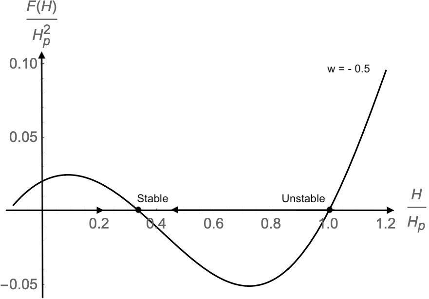
Figure 1: $\frac{3a_{1}^{2}}{4}=1$ is chosen.

The stable fixed point occurs when $0<H<H_{P}$, $F(H)$ has a ’future fixed point’ $H_{1}<H_{P}$. Since $F(H)$ is differentiable, the slope of the tangent at any fixed point is finite. Near the stable fixed point, $F(H)=F^{\prime}(H_{1})(H-H_{1})$ following [33]. Then the age of the universe

$$T\ =\ {\int}_{H_{0}}^{H_{1}}\frac{dH}{\dot{H}} = {\int}_{H_{0}}^{H_{1}}\ \frac{dH}{F^{\prime}(H_{1})(H-H_{1})}\ =\ \infty,$$ (38)

showing the universe had no beginning, consistent with the defocussing of world lines shown in [1]. Other allowed values of $\alpha$ and choice for $\frac{3a_{1}^{2}}{4}$ are found to be qualitatively similar without affecting the conclusion in (38). However, for other values of $\alpha$, the stable fixed point moves towards $H_{P}$ with $H_{1}$ coinciding with $H_{P}$. This is exhibited in Fig.2.

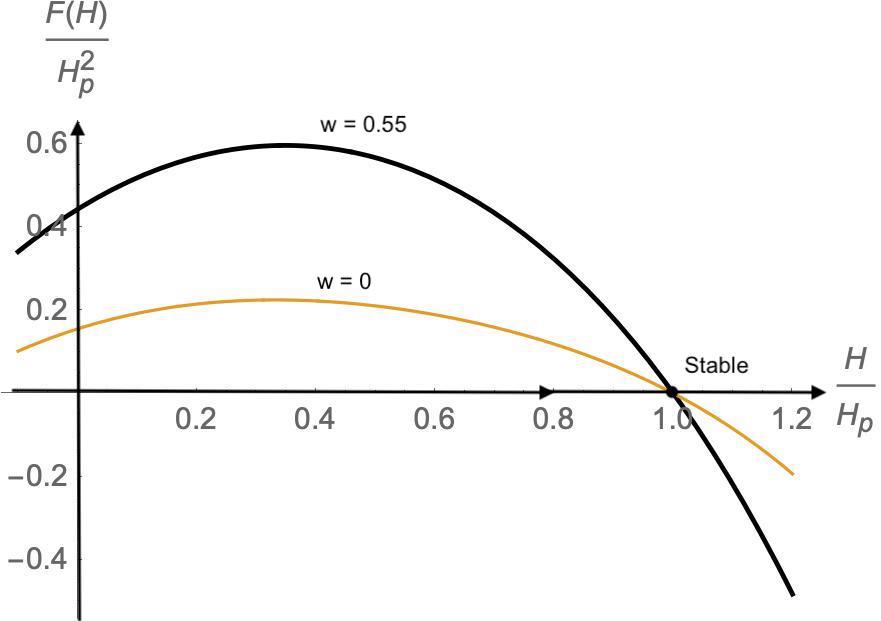
Figure 2: $\frac{3a_{1}^{2}}{4}=1$ is chosen.

In these cases also, the conclusion that $T\rightarrow\infty$ is obtained. Such a conclusion has been reached in [32] by considering quantum effects to Raychaudhuri equation. Here, the same conclusion is obtained using classical 5-d gravity for the description of the early universe.

6. Analysis of for $a(t)$:

The scale factor $a(t)$ in the flat FRW metric (7) satisfies (29), that is

$$a(t)\frac{d^{2}a(t)}{dt^{2}}+A\left(\frac{da(t)}{dt}\right)^{2}-\frac{3a_{1}^{2}}{4} = 0,$$ (39)

where $A=\frac{1}{8}(1+3w)$. We wish to solve the above equation for $a(t)$.

Solution.1:

By letting $a(t)={\psi(t)}^{\gamma}$, (39) becomes

$$\gamma(\gamma-1){\psi(t)}^{2\gamma-2}\left(\frac{d\psi}{dt}\right)^{2}+\gamma{\psi(t)}^{2\gamma-1}\frac{d^{2}\psi}{dt^{2}}+A{\gamma}^{2}{\psi(t)}^{2\gamma-2}\left(\frac{d\psi}{dt}\right)^{2}=\frac{3a_{1}^{2}}{4}.$$

Now, suppose we choose $\gamma=\frac{1}{1+A}$, then the above equation simplifies to

$${\psi(t)}^{\frac{1-A}{1+A}}\ \frac{d^{2}\psi}{dt^{2}} = \frac{3a_{1}^{2}}{4}(1+A).$$ (40)

By letting $\psi(t)=A_{1}(t+\epsilon)^{\rho}$ and taking $\rho=1+A$, we find

$$a(t) = \sqrt{\frac{3a_{1}^{2}}{4A}}\ (t+\epsilon).$$ (41)

It is to be noted with this exact solution of (39), the second derivative $\frac{d^{2}a(t)}{dt^{2}}$ vanishes. This solution exhibits classical bounce as $a(0)=\sqrt{\frac{3a_{1}^{2}}{4A}}\epsilon$. Further, this solution gives $\dot{H}=-H^{2}(t)=F(H)$ and the universe had a beginning.

Solution.2

By letting $W(t)={a(t)}^{A+1}$, the (39) becomes

$$\frac{d^{2}W(t)}{dt^{2}}-\frac{3a_{1}^{2}}{4}(A+1){W(t)}^{\frac{A-1}{A+1}} = 0.$$ (42)

Although the non-linearity in (39) is softened, it is still non-linear. As in the case of (28) for $H(t)$, we use iterative method. By neglecting the second term in (42), the solution of $\frac{d^{2}W(t)}{dt^{2}}=0$ gives $W(t)=\beta t+\gamma$ where $\beta$ and $\gamma$ are constants. using this for the second term in (42), we obtain

$$\frac{d^{2}W(t)}{dt^{2}} = \frac{3a_{1}^{2}}{4}(A+1)\left(\beta t+\gamma\right)^{\frac{A-1}{A+1}}.$$ (43)

This equation is integrated to give

$$W(t) = \frac{3a_{1}^{2}(A+1)^{3}}{4A(3A+1){\beta}^{2}}\left(\beta t+\gamma\right)^{\frac{3A+1}{A+1}}+C_{1}t+C_{2},$$ (44)

where $C_{1},C_{2}$ are constants. Then, the FRW scale factor is

$$a(t) = \left(\frac{3a_{1}^{2}(A+1)^{3}}{4A(3A+1){\beta}^{2}}\left(\beta\ t+\gamma\right)^{\frac{3A+1}{A+1}}+C_{1}t+C_{2}\right)^{\frac{1}{A+1}},$$ (45)

iterative solution for $a(t)$. When the scalar contribution is neglected (setting $a_{1}=0$), we see that $a(t)=\left(C_{1}\ t+C_{2}\right)^{\frac{1}{A+1}}$. With $a_{1}=0$, we should have standard cosmology for which $a(0)=0$ and so we choose $C_{2}=0$. With this choice, we have

$$a(t) = \left(\frac{3a_{1}^{2}(A+1)^{3}}{4A(3A+1){\beta}^{2}}\left(\beta t+\gamma\right)^{\frac{3A+1}{A+1}}+C_{1}\ t\right)^{\frac{1}{A+1}},$$ (46)

the behavior of the scale parameter $a(t)$. Now from this,

$$a(0) = \left(\frac{3a_{1}^{2}(A+1)^{3}}{4A(3A+1){\beta}^{2}}\right)^{\frac{1}{A+1}}\ {\gamma}^{\frac{3A+1}{(A+1)^{2}}},$$ (47)

showing classical bounce. It is to be noted that the bounce is proportional to $a$, the effect of the scalar in 5-d gravity in the early universe. Further from (46), we have expanding universe.

Solution.3. (Series solution),

In this method, the second derivative term in (39) is maintained. A series solution consists in taking

$$a(t) = b_{0}+b_{1}t+b_{2}t^{2}+b_{3}t^{3}+b_{4}t^{4}+\cdots$$ (48)

where $b_{0},b_{1},b_{2}\cdots$ are constants. Substituting in (39) and equating like powers of $t$, we obtain relations among these coefficients. From them, we consider three classes of solutions.

(1) If $b_{0}=0$, then, a solution $a(t)=\sqrt{\frac{3a_{1}^{2}}{4A}}t$ which correspond to the Solution.1 with $\epsilon=0$.

(2) If we choose, $b_{0}\neq 0;b_{1}\neq 0;b_{2}=0$, then a solution of $a(t)=b_{0}+\sqrt{\frac{3a_{1}^{2}}{4A}}t$ is obtained which is similar to Solution.1. Both these give $\dot{H}=-H^{2}$ same as in Solution.1.

(3) The third case corresponds to $b_{0}\neq 0;b_{1}=0$ and then the series solution corresponds to $a(t)=b_{0}+b_{2}t^{2}+b_{4}t^{4}+\cdots$, all even powers of $t$. The coefficients in this case are: $b_{2}=\frac{3a_{1}^{2}}{8b_{0}}$, $b_{4}=\frac{a_{1}^{2}}{16b_{0}}-\frac{3a_{1}^{4}(1+2A)}{128b_{0}^{3}}$ and so on. For illustrative purpose, we take $b_{0}=1$; $\frac{3a_{1}^{2}}{4}=1$ and $A=-\frac{1}{16}$ corresponding to $w=0.5$. Then, $H=\frac{t+0.16t^{3}}{1+0.5t^{2}+0.04t^{4}}$ and $\dot{H}=\frac{1+0.48t^{2}}{1+0.5t^{2}+0.04t^{4}}-H^{2}$, keeping upto $t^{4}$ in $a(t)$. From these, the graph connecting $\dot{H}$ with $H$ is drawn and this qualitatively gives Fig.2. In this third case, there is classical bounce as $a(0)\neq 0$.

Thus, the series method ensures departure from standard cosmology with classical bounce in agreement with the earlier analysis.

7. Summary:

We have extended our result on defocussing of world lines [1] by modifying gravity in the early epoch by a 5-d theory with scalar $\psi(r)$. The acceleration term in the Raychaudhuri equation has been shown to be positive for flat FRW metric. The scalar $\psi(r)$ satisfies a non-linear differential equation which is solved. Though singular, the acceleration term turns out to be finite. With this, the equations for the Hubble parameter $H(t)$ and the scale factor $a(t)$ are obtained. These are analyzed using ’fixed point analysis’. Without the scalar field, the age of the universe is finite showing a beginning of the universe and with out bounce. With the contribution of the scalar field included, the age of the universe is shown to be infinite, thereby resolving the singularity. The scale factor $a(t)$ exhibits classical bounce.

Acknowledgements:

We are thankful to Sonakshi Sachdev for help in drawing the figures. Useful discussions with Govind Krishnaswamy, B.V. Rao and K.S. Viswanathan are acknowledged with thanks.

References:

1. R.Parthasarathy, K.S.Viswanathan and Andrew DeBenedictis, Ann.Phys.398 (2018) 1.

2. R.Brandenberger and C.Vefa, Nucl.Phys. B316 (1989) 391.

3. M.Gasperini and G.Veneziano, Astro Particle Physics. 1 (1993) 317.

4. J.Khoury, B.A.Ovrut, P.J.Steinhardt and N.Turok, Phys.Rev. D64 (2001) 123522.

5. F.Finelli and R.Brandenberger, Phys.Rev. D65 (2002) 103522.

6. J.B.Hartle and S.W.Hawking, Phys.Rev. D28 (1983) 2960.

7. S.Gielen and N.Turok, Phys.Rev.Lett. 117 (2016) 021301.

8. M.Bojowald, Phys.Rev.Lett. 86 (2001) 5227.

9. A.Ashtekar, T.Pawlowski and P.Singh, Phys.Rev. D74 (2006) 084003.

10. S.Gielen and L.Sindoni, Quantum cosmology from group field theory condensates, arXiv 1602.08104.

11. M.de Caesare and M.Sakellariadov, Phys.Lett. B764 (2017) 49.

12. D.Oriti, L.Sindoni and E.Wilson-Ewing, Class.Quant.Gravity. 34 (2017) 04LT01.

13. M.Hohmann, L.Jarv and V.Valiklianova, Phys.Rev. D96 (2017) 043508,

14. S.D.Odintsov and V.K.Oikonomou, Int.J.Mod.Phys. D26 (2017) 1750085.

15. V.K.Oikonomov, Phys.Rev. D92 (2015) 124027.

16. K.Martineau and A.Barrau, Primordial power spectra from an emergent universe; basic results and clarfications, gr-qc/1812.05522.

17. R.Brandenberger and P.Peter, Bouncing cosmologies; Progress and Problems, hep-th/ 1603.05834.

18. A.M.Chamseddine and V.Mukhanov, Resolving cosmological singularities, gr-qc/1612.05860.

19. P.W.Graham, D.E.Kaplan and S.Rajendran, Phys.Rev. D97 (2018) 044003.

20. L.Annulli, V.Cardoso and L.Gualtieri, Electromagnetism and hidden vector fields in modified gravity theories, gr-qc/1901.02461.

21. A.K.Raychaudhuri, Phys,Rev. 98 (1955) 1123.

22. E.G. Mychelkin and M.A. Makukov, Unified geometrical basis for the generalized Ehlers identities and Raychaudhuri equations. gr-qc/1707.00862.

23. S. Ghosh, A. Dasgupta and S. Kar, Phys.Rev. D83 (2011) 084001.

24. J.M.Overduin and P.S.Wesson, Phys.Rep. 283 (1993) 303.

25. J. Borgman and L.H. Ford, Phys.Rev. D70 (2004) 064032.

26. E.F. Bunn, P. Ferriera and J. Silk, Phys.Rev.Lett. 77 (1996) 2883.

27. M.P. Hobson, G. Efstathiou and A.N. Lasenby, General Relativity: An Introduction for physicists, Cambridge University Press, 2006. Page.367.

28. F. De Felice and C.J.S. Clarke, Relativity on curved manifilds. Cambridge University Press, 1990.

29. J. Foster and J.D. Nightingle, A short course in General Relativity. Springer, 2006.

30. A.K.Raychaudhuri, Theoretical Cosmology, Oxford, U.K., 1979.

31. S.Das, Phys.Rev. D89 (2014) 084068.

32. A.F.Ali and S.Das, Phys.Lett. B741 (2016) 276.

33. A. Awad, Phys.Rev. D87 (2013) 103001. S.H. Strogatz, Nonlinear Dynamics and Chaos: Applications to Physics, Biology, Chemistry and Engineering, CRC Press, Taylor and Francis Group, A Chapman and Hall Book., 2018.

Appendix

Classical equation of motion for $\psi(r)$:

We start from the action (15) of [1]. After a partial integration of the second term (classical equation of motion will not be affected by having a total derivative), we have

$${\cal{S}} = \frac{1}{16\pi G_{4}}\int d^{4}x\sqrt{-g}\left(\sqrt{g_{55}}R-\frac{1}{2}g_{55}^{-\frac{3}{2}}g^{\mu\nu}({\partial}_{\mu}g_{55})({\partial}_{\nu}g_{55})\right),\hskip 56.9055pt(A1)$$

from which the Lagrangian density is

$${\cal{L}} = \sqrt{-g}\sqrt{g_{55}}R-\frac{1}{2}\sqrt{-g}g_{55}^{-\frac{3}{2}}g^{\mu\nu}({\partial}_{\mu}g_{55})({\partial}_{\nu}g_{55}).\hskip 113.81102pt(A2)$$

Then,

$$\frac{\partial{\cal{L}}}{\partial({\partial}_{\lambda}g_{55})} = -\sqrt{-g}g_{55}^{-\frac{3}{2}}g^{\lambda\mu}({\partial}_{\mu}g_{55}).$$

Using ${\partial}_{\lambda}(\sqrt{-g}g^{\lambda\mu})=-\sqrt{-g}{\Gamma}^{\mu}_{\alpha\beta}g^{\alpha\beta}$, it is seen that

$${\partial}_{\lambda}\left(\frac{\partial{\cal{L}}}{\partial({\partial}_{\lambda}g_{55})}\right) = \frac{3}{2}\sqrt{-g}g_{55}^{-\frac{5}{2}}g^{\lambda\mu}({\partial}_{\lambda}g_{55})({\partial}_{\mu}g_{55})-\sqrt{-g}g_{55}^{-\frac{3}{2}}g^{\alpha\beta}D_{\alpha}({\partial}_{\beta}g_{55}),$$

where $D_{\alpha}$ is the covariant derivative. Next,

$$\frac{\partial{\cal{L}}}{\partial g_{55}} = \frac{1}{2}\sqrt{-g}g_{55}^{-\frac{1}{2}}R+\frac{3}{4}\sqrt{-g}g_{55}^{-\frac{5}{2}}g^{\mu\nu}({\partial}_{\mu}g_{55})({\partial}_{\nu}g_{55}).\hskip 85.35826pt(A3)$$

From (3) and (4), the classical equation of motion for $g_{55}$ is

$$\frac{3}{4}g_{55}^{-\frac{5}{2}}g^{\mu\nu}({\partial}_{\mu}g_{55})({\partial}_{\nu}g_{55})-g_{55}^{-\frac{3}{2}}g^{\mu\nu}D_{\mu}({\partial}_{\nu}g_{55})-\frac{1}{2}g_{55}^{-\frac{1}{2}}R = 0.\hskip 56.9055pt(A4)$$

The 5-d Ricci scalar is zero and this gives $R=\frac{1}{g_{55}}g^{\mu\nu}D_{\mu}({\partial}_{\nu}g_{55})$. Using this in above, the classical equation of motion for $g_{55}$ becomes

$$g^{\mu\nu}D_{\mu}({\partial}_{\nu}g_{55})-\frac{1}{2}\frac{1}{g_{55}}g^{\mu\nu}({\partial}_{\mu}g_{55})({\partial}_{\nu}g_{55}) = 0.\hskip 113.81102pt(A5)$$

This agrees with Overduin and Wesson [22]. Now, using FRW metric, the equation of motion becomes with $g_{55}=\psi(r)$,

$$\frac{1}{2a^{2}(t)}\frac{1}{\psi}(\psi^{\prime})^{2}-\frac{1}{a^{2}(t)}\psi^{\prime\prime}-g^{\alpha\beta}{\Gamma}^{r}_{\alpha\beta}\psi^{\prime} = 0.\hskip 113.81102pt(A6)$$

For FRW, $g^{\alpha\beta}{\Gamma}^{r}_{\alpha\beta}=\frac{2}{ra^{2}(t)}$ and therefore, the above classical equation of motion becomes

$$\frac{2}{a^{2}(t)}\left(\frac{(\psi^{\prime})^{2}}{4\psi}-\frac{\psi^{\prime\prime}}{2}-\frac{\psi^{\prime}}{r}\right) = 0.\hskip 170.71652pt(A7)$$

This in turn implies that for FRW metric, $R_{55}=0$. So we need not impose $R_{55}=0$ as this becomes automatically zero by virtue of classical equation of motion for $\psi(r)$.