High-Dimensional Feature Selection for Genomic Datasets

Abstract

A central problem in machine learning and pattern recognition is the process of recognizing the most important features. In this paper, we provide a new feature selection method (DRPT) that consists of first removing the irrelevant features and then detecting correlations between the remaining features. Let $D=[A\mid\mathbf{b}]$ be a dataset, where $\mathbf{b}$ is the class label and $A$ is a matrix whose columns are the features. We solve $A\mathbf{x}=\mathbf{b}$ using the least squares method and the pseudo-inverse of $A$. Each component of $\mathbf{x}$ can be viewed as an assigned weight to the corresponding column (feature). We define a threshold based on the local maxima of $\mathbf{x}$ and remove those features whose weights are smaller than the threshold. To detect the correlations in the reduced matrix, which we still call $A$, we consider a perturbation $\tilde{A}$ of $A$. We prove that correlations are encoded in $\Delta\mathbf{x}=\mid\mathbf{x}-\tilde{\mathbf{x}}\mid$, where $\tilde{\mathbf{x}}$ is the least quares solution of $\tilde{A}\tilde{\mathbf{x}}=\mathbf{b}$. We cluster features first based on $\Delta\mathbf{x}$ and then using the entropy of features. Finally, a feature is selected from each sub-cluster based on its weight and entropy. The effectiveness of DRPT has been verified by performing a series of comparisons with seven state-of-the-art feature selection methods over ten genetic datasets ranging up from 9,117 to 267,604 features. The results show that, over all, the performance of DRPT is favorable in several aspects compared to each feature selection algorithm.

1 Introduction

Supervised learning is a central problem in machine learning and data mining [1]. In this process, a mathematical/statistical model is trained and generated based on a pre-defined number of instances (train data) and is tested against the remaining (test data). A subcategory of supervised learning is classification, where the model is trained to predict class labels [2]. For instance, in tumor datasets, class labels can be malignant or benign, the former being cancerous and the latter being non-cancerous tumors [3]. For each instance in a classification problem, there exists a set of features that contribute to the output [4].

In high-dimensional datasets, there are a large number of irrelevant features that have no correlation with the class labels. Irrelevant features act as noise in the data that not only increase the computational costs but, in some cases, divert the learning process toward weak model generation [5, 6]. The other important issue is the presence of correlation between good features, which makes some features redundant. Redundancy is known as multicollinearity in a broader context and it is known to create overfitting and bias in regression when a model is trained on data from one region and predicted on another region [7, 8].

The goal of feature selection (FS) methods is to select the most important and effective features [9]. As such, FS can decrease the model complexity in the training phase while retaining or improving the classification accuracy. Recent FS methods [10, 11, 12] usually find the most important features through a complex model which introduce a more complicated framework when followed by a classifier.

In this paper, we present a linear FS method called dimension reduction based on perturbation theory (DRPT). Let $D=[A\mid\mathbf{b}]$ be a dataset where $\mathbf{b}$ is the class label and $A$ is an $m\times n$ matrix whose columns are features. We shall focus on datasets where $m<<n$ and of particular interests to us are genomic datasets where gene expression level of samples (cases and controls) are measured. So, each feature is the expression levels of a gene measured across all samples. Biologically speaking, there is only a limited number of genes that are associated to a disease and, as such, only expression levels of certain genes can differentiate between cases and controls. So, a majority of genes are considered irrelevant. One of the most common methods to filter out irrelevant features in genomic datasets is using $p$-values. That is, one can look at the expression levels of a gene in normal and disease cases and calculate the $p$-values based on some statistical tests. It has been customary to conclude that genes whose $p$-values are not significant are irrelevant and can be filtered out. However, genes expressions are not independent events (variables) and researchers have been warned against the misuse of statistical significance and $p$-values, as it is recently pointed out in [13, 14].

We consider the system $A\mathbf{x}=\mathbf{b}$ where the rows of $A$ are independent of each other and $A\mathbf{x}=\mathbf{b}$ is an underdetermined linear system. This is the case for genomic datasets because each sample has different gene expressions from the others. Since $A\mathbf{x}=\mathbf{b}$ may not have a unique solution, instead we use the least squares method and the pseudo-inverse of $A$ to find the solution with the smallest 2-norm. One can view each component $x_{i}$ of $\mathbf{x}$ as an assigned weight to the column (feature) $\mathbf{F}_{i}$ of $A$. Therefore, the bigger the $|x_{i}|$ the more important $\mathbf{F}_{i}$ is in connection with $\mathbf{b}$.

It then makes sense to filter out those features whose weights are very small compared to the average of local maximums over $|x_{i}|$’s. After removing irrelevant features, we obtain a reduced dataset, which we still denote it by $[A\mid\mathbf{b}]$. In the next phase, we detect correlations between columns of $A$ by perturbing $A$ using a randomly generated matrix $E$ of small norm. Let $\tilde{\mathbf{x}}$ be the solution to $(A+E)\tilde{\mathbf{x}}=\mathbf{b}$. It follows from Theorem 3.3 that features $\mathbf{F}_{i}$ and $\mathbf{F}_{j}$ correlate if and only if $|x_{i}-\tilde{x}_{i}|$ and $|x_{j}-\tilde{x}_{j}|$ are almost the same. Next, we cluster $\Delta\mathbf{x}=|\mathbf{x}-\tilde{\mathbf{x}}|$ using a simplified least-squares method called Savitsky-Golay smoothing filter [15]. This process yields a step-wise function where each step is a cluster. We note that features in the same cluster do not necessarily correlate and so we further break up each cluster of $\Delta\mathbf{x}$ into sub-clusters using entropy of features. Finally, from each sub-cluster, we pick a feature and rank all the selected features using entropy.

The “stability” of a feature selection algorithm is recently discussed in [16]. An algorithm is ‘unstable’ if a small change in data leads to large changes in the chosen feature subset. In real datasets, it is possible that there are small noise or error involved in the data. Also, the order of samples (rows) in a dataset should not matter; the same applies to the order of features (columns). In Theorem 3.4 we prove that DRPT is noise-robust and in Theorem 3.5 we prove that DRPT is stable with respect to permuting rows or columns.

We compare our method with seven state-of-the-art FS methods, namely mRMR [17], LARS [18], HSIC-Lasso [19], Fast-OSFS [20], group-SAOLA [21], CCM [22] and BCOA [23] over ten genomic datasets ranging up from 9,117 to 267,604 features. We use Support Vector Machines (SVM) and Random Forest (RF) to classify the datasets based on the selected features by FS algorithms. The results show that, over all, the classification accuracy of DRPT is favorable compared with each individual FS algorithm. Also, we report the running time, CPU time, and memory usage and demonstrate that DRPT does well compared to other FS methods.

The rest of this paper is organized as follows. In Section 2, we review related work. We present our approach and the algorithm in Section 3. Experimental results and performance comparisons are shown in Section 4 and we conclude the paper in Section 5.

2 Related Work

FS methods are categorized as filter, wrapper and embedded methods [24]. Filter methods evaluate each feature regardless of the learning model. Wrapper-based methods select features by assessing the prediction power of each feature provided by a classifier. The quality of the selected subset using these methods is very high, but wrapper methods are computationally inefficient. The last group consolidates the advantages of both methods, where a given classifier selects the most important features simultaneously with the training phase. These methods are powerful, but the feature selection process cannot be defused from the classification process.

Providing the most informative and important features to a classifier would result in a better prediction power and higher accuracy [25]. Selecting an optimal subset of features is an NP-hard problem that has attracted many researchers to apply meta-heuristic and stochastic algorithms [26, 27, 28].

Several methods exist that aim to enhance classification accuracy by assigning a common discriminative feature set to local behavior of data in different regions of the feature space [29, 30]. For example, localized feature selection (LFS) is introduced by Armanfard et al. [30], in which a set of features is selected to accommodate a subset of samples. For an arbitrary query of the unseen sample, the similarity of the sample to the representative sample of each region is calculated, and the class label of the most similar region is assigned to the new sample.

On the other hand, some approaches use aggregated sample data to select and rank the features [17, 18, 19, 31, 32]. The least absolute shrinkage and selection operator (LASSO) is an estimation method in linear models which simultaneously applies variable selection by setting some coefficients to zero [31].

Least angle regression (LARS) proposed by Efron et al. [18] is based on LASSO and is a linear regression method which computes all least absolute shrinkage and selection operator [31] estimates and selects those features which are highly correlated to the already selected ones.

Chen et al. [32] introduced a semi-supervised FS called Rescaled Linear Square Regression (RLSR), in which rescaling factors are incorporated to exploit the least square regression model and rank features. They solve the minimization problem shown in equation 1 to learn $\mathbf{\Theta}$ and $\mathbf{Y}_{U}$, which are a matrix of rescaling factors and unknown labels, respectively.

$$\min\Big{(}||\mathbf{X}^{T}\mathbf{\Theta}\mathbf{W}+\mathbf{1b}^{T}-\mathbf{Y}||^{2}_{F}+\gamma||\mathbf{W}||^{2}_{F}\Big{)}\\ \text{st.}\mathbf{W},\mathbf{b},\theta>0,\mathbf{1}^{T}\theta=1,\mathbf{Y}_{U}\geq 0,\mathbf{Y}_{U}\mathbf{1}=\mathbf{1},$$ (1)

where $\mathbf{W}$ is a sparse matrix that represents the importance of features, $\mathbf{X}$ is the dataset, $\mathbf{Y}$ is class labels, and $b=\frac{1}{n}(\mathbf{Y}^{T}\mathbf{1}-\mathbf{W}^{T}\mathbf{X}\mathbf{1})$, where $n$ is number of samples in a dataset. Their proposed algorithm continuously updates $\mathbf{W}$, $\mathbf{b}$ and $\mathbf{Y}_{U}$ until convergence.

Yamada et al. [19] proposed a non-linear FS method for high-dimensional datasets called Hilbert-Schmidt independence criterion least absolute shrinkage and selection operator (HSIC-Lasso), in which the most informative non-redundant features are selected using a set of kernel functions, where the solutions are found by solving a LASSO problem. The complexity of the original Hilbert-Schmidt FS (HSFS) is $O(n^{4})$. In a recent work [33] called Least Angle Nonlinear Distributed (LAND), the authors have improved the computational power of the HSIC-Lasso. They have demonstrated via some experiments that LAND and HSIC-Lasso attain similar classification accuracies and dimension reduction. However, LAND has the advantage that it can be deployed on parallel distributed computing. Another kernel-based feature selection method is introduced in [22] using measures of independence and minimizing the trace of the conditional covariance operator. It is motivated by selecting the features that maximally account for the dependence on the covariates’ response.

In some recent real-world applications, we need to deal with sequentially added dimensions in a feature space while the number of data instances is fixed. Yu et al. [34] developed an open source Library of Online FS (LOFS) using state-of-the-art algorithms. The learning module of LOFS consists of two submodules, Learning Features added Individually (LFI) and Learning Grouped Features added sequentially (LGF). The LFI module includes various FS methods including Alpha-investing [35], OSFS [36], Fast-OSFS [20], and SAOLA [37] to learn features added individually over time, while the LGF module provides the group-SAOLA algorithm [21] to mine grouped features added sequentially.

In [38], the authors proposed a bio-inspired optimization algorithm called Coyote Optimization Algorithm (COA) simulating the behavior of coyotes. Using their new strategy, COA makes a balance between exploration and exploitation processes to solve continuous optimization problems. Very recently, the authors [23] upgraded their method by proposing a binary version of COA called Binary Coyote Optimization Algorithm (BCOA), which is a wrapper feature selection method.

There is a great interest in the applications of FS methods in disease diagnoses and prognoses. For example, Parkinson’s disease (PD) is a critical neurological disorder and its diagnoses in its initial stages is extremely complex and time consuming. Recently, voice recordings and handwritten drawings of PD patients are used to extract a subset of important features using FS algorithms to diagnose PD [39, 40, 41, 42, 43] with a good success rate.

3 Proposed approach

Consider a dataset $D$ consisting of $m$ samples where each sample contains $n+1$ features. Let us denote by $A$ the first $n$ columns of $D$ and by $\mathbf{b}$ the last column. We also denote by $\mathbf{F}_{i}$ the $i$-th feature (column) of $A$. We shall first consider eliminating the irrelevant features. Throughout, by the norm of a vector, we always mean its 2-norm. Recall that

$$||A||=\text{Sup}_{\mathbf{x}\neq 0}\frac{||A\mathbf{x}||}{||\mathbf{x}||}=\text{Sup}_{||\mathbf{x}||=1}||A\mathbf{x}||$$

Denote by $\sigma_{1}\geq\sigma_{2}\geq\cdots\geq\sigma_{r}$ the singular values of $A$, where $r=\text{min}(m,n)$. The smallest non-zero singular value of $A$ is denoted by $\sigma_{\text{min}}$ and the greatest of the $\sigma_{i}$ is also denoted by $\sigma_{\text{max}}$. It is well-known that $||A||_{2}=\sigma_{\text{max}}$. Recall that $A$ admits a singular value decomposition (SVD) in the form $A=U\Sigma V^{T}$, where $U$ and $V$ are orthogonal matrices and $\Sigma=\text{diag}(\sigma_{1},\ldots,\sigma_{r},0,\ldots,0)$ is an $m\times n$ diagonal matrix. Here, $V^{T}$ denotes the transpose of $V$.

We first normalize the columns of $A$ so that each $\mathbf{F}_{i}$ has norm 1. Then, we solve the linear system $A\mathbf{x}=\mathbf{b}$ by using the method of least squares (see theorem 3.1). Here, $\mathbf{x}=[x_{1}\cdots x_{i}\cdots x_{n}]^{T}$. The idea is to select a small number of columns of $A$ that can be used to approximate $\mathbf{b}$. Since $A\mathbf{x}=\mathbf{b}$ may not have a unique solution, instead we consider a broader picture by solving the least squares problem $\text{min}_{\mathbf{x}}||A\mathbf{x}-\mathbf{b}||_{2}$ whose solution is given in terms of pseudo-inverse and SVD of $A$. The following result is well-known, see [44].

Theorem 3.1 (All Least Squares Solutions)

Let $A$ be an $m\times n$ matrix and $\mathbf{b}\in\mathbb{R}^{m}$. Then all the solutions of $\text{min}_{\mathbf{x}}||A\mathbf{x}-\mathbf{b}||_{2}$ are of the form $\mathbf{y}=A^{+}\mathbf{b}+\mathbf{z}$, where $\mathbf{z}\in\ker(A)$. Furthermore, the unique solution whose 2-norm is the smallest is given by $\mathbf{x}=A^{+}\mathbf{b}$.

In other words, we can approximate the label column $\mathbf{b}$ as a linear combination $x_{1}\mathbf{F}_{1}+\cdots+x_{n}\mathbf{F}_{n}$. So each $|x_{i}|$ can be viewed as an assigned weight to $\mathbf{F}_{i}$. Given that each $\mathbf{F}_{i}$ has norm 1, if $|x_{i}|$ is small compared to others, then the vector $x_{i}\mathbf{F}_{i}$ will have a negligible effect on $\mathbf{b}$. It then makes sense to filter out those features whose weights are very small. In other words, we shrink the weights of irrelevant features to zero.

In this paper, we shall mostly focus on datasets where $m<<n$. Of special interest to us are genomic datasets where there are usually tens or hundreds of samples compared to tens of thousands of genes. The matrix $A$ in these datasets has full row-rank because gene expressions of different samples are independent of each other. Since $\mathbf{b}\in\mathbb{R}^{m}$, it is enough to identify only $m$ independent columns of $A$. Intuitively, it makes sense to eliminate the columns that are less important.

We prove below how weight of each feature $\mathbf{F}_{i}$ is directly affected by the relevance of $\mathbf{F}_{i}$ to $\mathbf{b}$. Suppose that $A$ is an $m\times n$ of full row-rank and consider the SVD of $A$ as $A=U\Sigma V^{T}$. Let $U=\left[\begin{array}[]{c|c|c}\mathbf{u}_{1}&\cdots&\mathbf{u}_{m}\end{array}\right]$. Note that $\mathbf{u}_{1},\ldots,\mathbf{u}_{m}$ form an orthonormal basis of $\mathbb{R}^{m}$.

Theorem 3.2

Let $A$ be a full row-rank matrix and denote by $\mathbf{x}=[x_{1}\ldots x_{n}]^{T}$ the least squares solutions to $A\mathbf{x}=\mathbf{b}$. Then, each component $x_{i}$ of $\mathbf{x}$ is given by $x_{i}=\langle\mathbf{F}_{i},\mathbf{z}\rangle$, where $\mathbf{z}=U[\langle\mathbf{u}_{1},\mathbf{b}\rangle/\sigma_{1}^{2}\,\cdots\,\langle\mathbf{u}_{m},\mathbf{b}\rangle/\sigma_{m}^{2}]^{T}$.

Proof. Since $A$ is full row-rank, the right inverse of $A$ is $A^{+}=A^{T}(AA^{T})^{-1}$. Consider the SVD of $A$ as $A=U\Sigma V^{T}$. Then $AA^{T}=U\Sigma\Sigma^{T}U^{T}=\sum_{i=1}^{m}\sigma_{i}^{2}u_{i}u_{i}^{T}$. Note that the solution of $A\mathbf{x}=\mathbf{b}$ with the smallest norm is $\mathbf{x}=A^{+}\mathbf{b}=A^{T}(AA^{T})^{-1}\mathbf{b}$. Let $\mathbf{z}=(AA^{T})^{-1}\mathbf{b}$. So, $\mathbf{b}=AA^{T}\mathbf{z}=\sum_{i=1}^{m}\sigma_{i}^{2}u_{i}u_{i}^{T}\mathbf{z}$. Since the $\mathbf{u}_{i}$s are orthonormal, we get

$$\langle\mathbf{u}_{k},\mathbf{b}\rangle=\sigma_{k}^{2}\langle\mathbf{u}_{k},\mathbf{z}\rangle,\quad k=1,\ldots,m.$$ (2)

Since $A$ has full row-rank, we have $\sigma_{k}>0$, for all $k$. Let $\bar{b}_{1},\ldots,\bar{b}_{m}$ be the coordinates of $\mathbf{b}$ with respect to the basis $\mathbf{u}_{1},\ldots,\mathbf{u}_{m}$ of $\mathbb{R}^{m}$. Similarly, let $\bar{z}_{1},\ldots,\bar{z}_{m}$ be the coordinates of $\mathbf{z}$ with respect to this basis. So, $\mathbf{b}=U[\bar{b}_{1}\,\ldots\,\bar{b}_{m}]^{T}$ and $\mathbf{z}=U[\bar{z}_{1}\,\ldots\,\bar{z}_{m}]^{T}$. Equation (2) can be written as $\bar{b}_{k}=\sigma_{k}^{2}\bar{u}_{k}$, for each $1\leq k\leq m$. On the other hand, $\mathbf{x}=A^{+}\mathbf{b}=A^{T}(AA^{T})^{-1}\mathbf{b}=A^{T}\mathbf{z}$. Since $\mathbf{z}=U[\bar{z}_{1}\,\ldots\,\bar{z}_{m}]^{T}$, we deduce that $x_{i}=\langle\mathbf{F}_{i},\mathbf{z}\rangle$, for each $i$. $\Box$

We note that the extent to which a feature is relevant to $\mathbf{b}$ also depends on how important the other features are in determining $\mathbf{b}$. This fact is reflected in Theorem 3.2 by taking into account the singular values of $A$ that encode part of the information about $A$. Also, the definition of relevancy is not quantitative and one has to set a threshold for the degree of relevancy. We set a dynamic threshold by calculating the average of all local maxima in $\mathbf{x}$ and remove those features that their corresponding value $|x_{i}|$ is smaller than the threshold. In a sense, the threshold is set so that rank of the reduced matrix is still the same as of the original $A$. So, in the reduced matrix, we only keep features that have a higher impact on $\mathbf{b}$ and yet the reduced matrix retains the same prediction power as $A$ in approximating $\mathbf{b}$.

If $A$ is full row-rank then, it follows from Theorem 3.1 that the solution $\mathbf{x}^{R}$ of smallest 2-norm to the system $A\mathbf{x}=\mathbf{b}$ is in the row space of $A$. So, there is a vector $\mathbf{y}$ such that $\mathbf{x}^{R}=-A^{T}\mathbf{y}$. Hence, $\mathbf{x}^{R}$ satisfies $\mathbf{x}^{R}+A^{T}\mathbf{y}=0,A\mathbf{x}^{R}=\mathbf{b}$. In other words, $\mathbf{x}^{R}$ is part of the solution to the non-singular linear system

$$\left(\begin{array}[]{ c c }I&A^{T}\\ A&0\end{array}\right)\left(\begin{array}[]{ c c }x^{R}\\ y\end{array}\right)=\left(\begin{array}[]{ c c }0\\ b\end{array}\right)$$

Next, we show how we can detect correlations between features. Recall that a perturbation of $A$ is of the form $A+E$, where $E$ is a random matrix with the normal distribution. We choose $E$ to be a random matrix such that $||E||_{2}\approx 10^{-s}\sigma_{\text{min}}(A)$, for some $s\geq 0$. We set $s=3$ where our estimates are correct up to a magnitude of $10^{-3}$.

Theorem 3.3

Let $\mathbf{x}$ and $\mathbf{{\tilde{x}}}$ be solutions of $A\mathbf{x}=\mathbf{b}$ and $(A+E)\mathbf{{\tilde{x}}}=\mathbf{b}$, where $E$ is a perturbation such that such that $||E||_{2}=10^{-s}\sigma_{\text{min}}(A)$. If a feature $\mathbf{F}_{i}$ is independent of the rest of the features, then $|x_{i}-\tilde{x}_{i}|\approx 0$. Furthermore, suppose that features $\mathbf{F}_{j}$ and $\mathbf{F}_{k}$ correlate, say $\mathbf{F}_{j}=c\mathbf{F}_{k}$ for some scalar $c$. If $\mathbf{F}_{j}$ and $\mathbf{F}_{k}$ are independent from the rest of the features, then $c=\frac{x_{k}-\tilde{x}_{k}}{x_{j}-\tilde{x}_{j}}$.

Proof. From $A\mathbf{x}=\mathbf{b}$ and $(A+E)\mathbf{{\tilde{x}}}=\mathbf{b}$, we get $A(\mathbf{x}-\mathbf{{\tilde{x}}})=E\mathbf{{\tilde{x}}}$. Consider the SVD of $A+E$ which is of the form $A+E=U\Sigma V^{T}$. So, $\mathbf{{\tilde{x}}}=V\Sigma^{-1}U^{T}\mathbf{b}$. Since $U$ and $V$ are orthogonal and for orthogonal matrices we have $||U\mathbf{v}||_{2}=||\mathbf{v}||_{2}$, we get

$$||\mathbf{{\tilde{x}}}||_{2}=||V\Sigma^{-1}U^{T}\mathbf{b}||_{2} =||\Sigma^{-1}\mathbf{b}||_{2}$$

$$\leq||\Sigma^{-1}||_{2}||\mathbf{b}||_{2}=\frac{1}{\sigma_{\text{min}}(A+E)}$$

$$\leq\frac{1}{-||E||_{2}+\sigma_{\text{min}}(A)}.$$

Hence, $||E\mathbf{{\tilde{x}}}||_{2}\leq||E||||\mathbf{{\tilde{x}}}||_{2}\leq 10^{-s}$ and we deduce that

$$(x_{1}{-}\tilde{x}_{1})\mathbf{F}_{1}+\cdots+(x_{t}{-}\tilde{x}_{t})\mathbf{F}_{t}+\cdots+(x_{n}{-}\tilde{x}_{n})\mathbf{F}_{n}\approx 0.$$

Now, if a feature, say $\mathbf{F}_{i}$, is independent of the rest of features, then it follows that $|x_{i}-\tilde{x}_{i}|\approx 0$. Furthermore, since $\mathbf{F}_{j}$ and $\mathbf{F}_{k}$ are independent from the rest of the features, we must have

$$(x_{j}-\tilde{x}_{j})\mathbf{F}_{j}+(x_{k}-\tilde{x}_{k})\mathbf{F}_{k}\approx 0.$$

So, $\mathbf{F}_{j}=\frac{x_{k}-\tilde{x}_{k}}{x_{j}-\tilde{x}_{j}}\mathbf{F}_{k}$. Hence, $c=\frac{x_{k}-\tilde{x}_{k}}{x_{j}-\tilde{x}_{j}}$, as required. $\Box$

Theorem 3.3 shows how we can filter out irrelevant features by looking at the components of $\mathbf{x}-\mathbf{\tilde{x}}$ that are close to zero. Also, as we mentioned before, we normalize the columns of $A$ so that each $\mathbf{F}_{i}$ has norm 1. So, if in the raw dataset $\mathbf{F}_{j}$ and $\mathbf{F}_{k}$ correlate then after normalization we must have $\mathbf{F}_{j}^{\prime}=\pm\mathbf{F}_{k}^{\prime}$. Here, $\mathbf{F}_{j}^{\prime}=\frac{\mathbf{F}_{j}}{||\mathbf{F}_{j}||}$. So, by Theorem 3.3, if $\mathbf{F}_{j}$ and $\mathbf{F}_{k}$ are independent from other features, we must have $|x_{k}-\tilde{x}_{k}|=|x_{j}-\tilde{x}_{j}|$. We explain these notions further in a synthetic dataset. Consider a synthetic dataset with 22 features and 100 samples and the label column $\mathbf{b}$ which we set as $\mathbf{b}=3\mathbf{F}_{19}+5\mathbf{F}_{17}+2\mathbf{F}_{20}$. The first 20 features of this dataset are generated randomly in the interval of -1 and 1. The correlations between remaining features are set as follows: $\mathbf{F}_{21}=2\mathbf{F}_{18}+4\mathbf{F}_{19}$ and $\mathbf{F}_{22}=3\mathbf{F}_{20}$. First, we normalize $A$. Then solve $A\mathbf{x}=\mathbf{b}$ and $(A+E)\mathbf{\tilde{x}}=\mathbf{b}$ and calculate $\Delta\mathbf{x}$ as shown in Table 1.

Table 1: Perturbation of the synthetic Dataset

	x	$\tilde{\mathbf{x}}$	$\Delta\mathbf{x}=|\mathbf{x}-\mathbf{\tilde{x}}|$
$\mathbf{F}_{1}$…$\mathbf{F}_{16}$	$\leq$3.0987e-14	$\leq$2.6907e-05	$\leq$4.7316e-05
$\mathbf{F}_{17}$	29.1715	29.1715	2.7239e-05
$\mathbf{F}_{18}$	-3.4494	-10.2466	6.7972
$\mathbf{F}_{19}$	9.9339	-3.1806	13.1145
$\mathbf{F}_{20}$	-5.3307	-6.0073	0.6766
$\mathbf{F}_{21}$	7.3630	21.8723	14.5093
$\mathbf{F}_{22}$	-5.3307	-4.6541	0.6766

Let $\Delta\mathbf{x}=|\mathbf{x}-\tilde{\mathbf{x}}|$ and denote its $i$-th component with $\Delta x_{i}$. Since each of $\mathbf{F}_{1},\ldots,\mathbf{F}_{17}$ are independent from the other features, as we expected, we have $\Delta x_{i}\approx 0$, for all $1\leq i\leq 17$. However, $\mathbf{F}_{17}$ is relevant because it correlates with $\mathbf{b}$. Indeed, $\mathbf{F}_{17}$ is a very important feature because we cannot make up for its loss using other features. Hence, we should be able to distinguish and preserve $\mathbf{F}_{17}$ from other $\mathbf{F}_{i}$ for which $\Delta x_{i}=0$. This can be accomplished by noting that irrelevant features have smaller $|x_{i}|$ compared to other features as can be seen from Table 1.

Since $\mathbf{F}_{22}=3\mathbf{F}_{20}$, these features correlate and are independent from other features. By normalization, we get $\mathbf{F}_{22}^{\prime}=\mathbf{F}_{20}^{\prime}$. So, we expect to have $\Delta x_{20}\approx\Delta x_{22}$ as shown in Table 1. We deduce that $\mathbf{F}_{22}$ and $\mathbf{F}_{20}$ are dependent and so we should only choose one of them.

Finally, after normalization and rewriting the relation $\mathbf{F}_{21}=2\mathbf{F}_{18}+4\mathbf{F}_{19}$, we obtain $\mathbf{F}_{21}^{\prime}\approx\mathbf{F}_{19}^{\prime}$ modulo $\mathbf{F}_{18}^{\prime}$. The reason for this is because norms of $\mathbf{F}_{21}^{\prime}$ and $\mathbf{F}_{19}^{\prime}$ outweigh norm of $\mathbf{F}_{18}^{\prime}$. This is confirmed in Tabel 1 as $\Delta x_{19}$ and $\Delta x_{21}$ are closest to each other compared to the others. So, $\mathbf{F}_{19}$ and $\mathbf{F}_{21}$ fall into the same cluster of $\Delta\mathbf{x}$. This means that one of $\mathbf{F}_{19}$ or $\mathbf{F}_{21}$ must be removed as a redundant feature. We shall now explain the clustering process of $\Delta\mathbf{x}$.

By Theorem 3.3, if features $\mathbf{F}_{i}$ and $\mathbf{F}_{j}$ correlate, then the differences $\Delta x_{i}$ and $\Delta x_{j}$ are almost the same. That is, the correlations between features are encoded in $\Delta\mathbf{x}$. Now, we sort $\Delta\mathbf{x}$ and obtain a stepwise function where each step can be viewed as a cluster consisting of features that possibly correlate with each other. To find an optimal number of steps, it makes sense to smooth $\Delta\mathbf{x}$ where we view $\Delta\mathbf{x}$ as a signal and use a simplified least-squares method called Savitsky-Golay smoothing filter [15]. Figure 1 exhibits how the smoothening process on $\Delta\mathbf{x}$ preserves its whole structure without changing the trend.

We note that the converse of Theorem 3.3 may not be true in general. That is $\Delta x_{i}$ and $\Delta x_{j}$ being the same does not necessarily imply that $\mathbf{F}_{i}$ and $\mathbf{F}_{j}$ correlate. Hence, in the next step, we want to further break up each cluster of $\Delta\mathbf{x}$ into sub-clusters. There are several ways to accomplish this step and one of the most natural ways is to use entropy of features.

Generally, entropy is a key measure for information gain and it is capable of quantifying the disorder or uncertainty of random variables. Also, entropy effectively scales the amount of information that is carried by random variables. Entropy of a feature $\mathbf{F}$ is defined as follows:

$$H(\mathbf{F})=-\sum_{k=1}^{m}{f_{k}\log f_{k}}$$ (3)

where $m$ is the number of samples and $f_{k}$ is the frequency with which $\mathbf{F}$ assumes the $k$-th value in the observations.

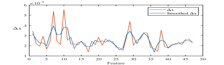
Figure 1: $\Delta\mathbf{x}$ vs. smoothed $\Delta\mathbf{x}$

Figure 2(a) shows clustering the set of all features based on $\Delta\mathbf{x}$, and then a typical cluster splits into sub-clusters using entropy as shown in Figure 2(b). To do so, we sort the features of a cluster based on their entropy which yields another step-wise function. At this stage, we pick one candidate feature from each sub-cluster based on the corresponding values $|x_{i}|$. Finally, the selected features are ranked based on both their entropies and the corresponding $|x_{i}|$’s. The final sorting of the features is an amalgamation of these two rankings.

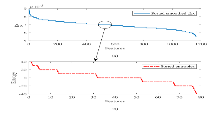
Figure 2: (a) Sorted smoothed $\Delta\mathbf{x}$ (b) Sorted entropies of the magnified cluster

3.1 Noise-robustness and stability

In real datasets, it is likely that $D$ involves some noise. For example, in genomics, it is conceivable that through the process of preparing a genomic dataset, some error/noise is included and as such the dataset $D$ is noisy. We note that the label column $\mathbf{b}$ is already known to us (and without noise). So instead of $D=[A\mid\mathbf{b}]$ we deal with $D=[A_{1}\mid\mathbf{b}]$, where $A_{1}=A+E_{1}$ and $||E_{1}||_{2}$ is small ($||E_{1}||_{2}=10^{-s}\sigma_{\text{min}}(A)$). A perturbation of $A_{1}$ is of the form $\tilde{A}_{1}=A_{1}+E_{2}$, where $||E_{2}||_{2}=10^{-s}\sigma_{\text{min}}(A)$. Our aim is to show that if certain columns of $A$ correlate, then so do the same columns of $A_{1}$ and vice versa.

Theorem 3.4

Let $\tilde{\mathbf{x}},{\mathbf{\tilde{y}}}$ be solutions of $A_{1}\tilde{\mathbf{x}}=\mathbf{b}$ and $\tilde{A}_{1}{\mathbf{\tilde{y}}}=\mathbf{b}$, respectively. Suppose that $S^{\prime}=\{\mathbf{F}_{1},\ldots,\mathbf{F}_{t}\}$ is set of columns of $A$ such that $\sum_{i=1}^{t}c_{i}\mathbf{F}_{i}=0$, for some non-zero $c_{i}$. If

1. any subset of $S^{\prime}$ is linearly independent,

2. $\mathbf{F}_{1},\ldots,\mathbf{F}_{t}$ are linearly independent from the remaining columns of $A$.

Then the vectors $\begin{bmatrix}c_{1}&\cdots&c_{t}\end{bmatrix}$ and $\begin{bmatrix}\tilde{x}_{1}-\tilde{y}_{1}&\cdots&\tilde{x}_{t}-\tilde{y}_{t}\end{bmatrix}$ are proportional.

Proof. From $(A+E_{1})\tilde{\mathbf{x}}=\mathbf{b}$ and $(A+E_{1}+E_{2})\tilde{\mathbf{y}}=\mathbf{b}$, we get $A(\tilde{\mathbf{x}}-\tilde{\mathbf{y}})=-E_{1}\tilde{\mathbf{x}}_{1}+(E_{1}+E_{2})\tilde{\mathbf{y}}$. Similar arguments as in the proof of Theorem 3.3 can be used to show that

$$||-E_{1}\tilde{\mathbf{x}}+(E_{1}+E_{2})\tilde{\mathbf{y}}|| \leq||-E_{1}\tilde{\mathbf{x}}_{1}||+||(E_{1}+E_{2})\tilde{\mathbf{y}}||$$

$$\leq\frac{1}{10^{s}-1}+\frac{2\cdot 10^{-s}}{-2\cdot 10^{-s}+1}$$

$$\leq\frac{1}{10^{s}-1}+\frac{2}{10^{s}-2}$$

$$\approx 3\cdot 10^{-s}$$

We deduce that

$$(\tilde{x}_{1}-\tilde{y}_{1})\mathbf{F}_{1}+\cdots+(\tilde{x}_{t}-\tilde{y}_{t})\mathbf{F}_{t}+\cdots+(\tilde{x}_{n}-\tilde{y}_{n})\mathbf{F}_{n}\approx 0.$$ (4)

Since $\mathbf{F}_{1},\ldots,\mathbf{F}_{t}$ are linearly independent from the rest of features in $S$, we get

$$(\tilde{x}_{1}-\tilde{y}_{1})\mathbf{F}_{1}+\cdots+(\tilde{x}_{t}-\tilde{y}_{t})\mathbf{F}_{t}\approx 0.$$ (5)

Now, if $\begin{bmatrix}c_{1}&\cdots&c_{t}\end{bmatrix}$ and $\begin{bmatrix}\tilde{x}_{1}-\tilde{y}_{1}&\cdots&\tilde{x}_{t}-\tilde{y}_{t}\end{bmatrix}$ are not proportional, we can use Equation (5) and our first hypothesis to get a dependence relation of a shorter length between the elements of $S^{\prime}$, which would contradict our assumption that any proper subset of $S^{\prime}$ is linearly independent. The proof is complete. $\Box$

We also remark that our method is insensitive to shuffling of the dataset $D$. That is, if we exchange rows (or columns), there is an insignificant change in $\Delta\mathbf{x}$. We have demonstrated this fact through experiments in Tables 4; we offer a proof as follows.

Theorem 3.5

DRPT is insensitive to permuting rows or columns.

Proof. We show this for permutation of rows and a similar argument can be made for permuting columns. Suppose that $D_{1}=[A_{1}\mid\mathbf{b}_{1}]$ is obtained from $D$ by shuffling rows. First, assume that only two rows are exchanged. Then there exists an elementary matrix $T$ such that $TA=A_{1}$ and $T\mathbf{b}=\mathbf{b}_{1}$. Since $T$ is invertible, it follows that $A\mathbf{x}=\mathbf{b}$ if and only if $A_{1}\mathbf{x}=\mathbf{b}_{1}$. For the general case, we note that every shuffling is a composition of elementary matrices.

3.2 Algorithm

The Flowchart and algorithm of DRPT are as follows. The MATLAB^®implementation of DRPT is publicly available in GitHub .

Figure 3: Flowchart of Dimension Reduction based on Perturbation Theory (DRPT)

Algorithm 1 Dimension reduction based on perturbation theory (DRPT)

Input: $D=[A\mid\textbf{b}],k$

Output: A subset of features of size $k$

$\triangleright$ //***Part1: Irrelevant Feature Removal***                    

Normalize columns of $A$ within $[0,1]$

$\textbf{x}=A^{+}\textbf{b}$

$\text{TH}=$Average(LocalMaxima of x)

$I=\emptyset$

for each $x_{i}\in$ x do

     if $x_{i}\geq\text{TH}$ then

         $I=I\cup{i}$      

$A\leftarrow A[I]$

$\triangleright$ //***Part2: Detecting Correlations***                      

$s=3$

$(m,n)=\text{Size}(A)$

$minSVD=Min$(singular value of $A$)

$\textbf{x}=A^{+}\textbf{b}$

$t=10^{-s}\cdot minSVD$

Set $E$ be a random $m\times n$ matrix with uniform dist. in the interval (0,1)

$E=t.*E$

$\tilde{A}=A+E$

$\Delta\textbf{x}=|(\tilde{A})^{+}\textbf{b}-\textbf{x}|$

$\Delta\textbf{x}=\text{Smooth}(\Delta\textbf{x})$

$\triangleright$ //***Part3: Ranking Features***                            

while  $z\in\text{unique}(\Delta\textbf{x})$  do

     $\text{CL}=\{\textbf{F}_{i}\mid|x_{i}-\tilde{x}_{i}|=z$}

     for  $h\in\text{unique}(H(\text{CL}))$ do

         $\text{subCL}=\{\textbf{F}_{i}\in\text{CL}\mid H(\textbf{F}_{i})=h\}$

         $\text{Pick }\textbf{F}_{i}\text{ in subCL with }|x_{i}|=\max\textbf{x}_{\text{subCL}}$

         $\text{Output}\leftarrow\text{Output}\cup\textbf{F}_{i}$      

$Ranked$ $Output$ $\leftarrow$ Rank ($Output$, {$H(F)$ & x})

Return: the top $k$ features

3.3 Complexity

The complexity of our proposed method is dominated by the complexity of the SVD which is $O(mn^{2},m^{2}n)$, since the inverse of perturbed $\tilde{A}$ is calculated using SVD.

4 Experimental Results

We compared our method with seven state-of-the-art FS methods, namely minimal-redundancy-maximal-relevance criterion (mRMR) [17], least angle regression (LARS) [18], Hilbert-Schmidt Independence Criterion Lasso (HSIC-Lasso) [19], Fast Online Streaming FS (Fast-OSFS) and Scalable, Accurate Online FS (group-SAOLA) [34], Conditional Covariance Minimization (CCM) [22] and Binary Coyote Optimization Algorithm (BCOA) [23] . We used MATLAB ^®implementations of LARS and LASSO by Sjöstrand [45], HSIC-Lasso and BCOA by their authors, Fast-OSFS and group-SAOLA given in the open source library [34]. The CCM method is implemented in Python by their authors and its code available at GitHub.

To have a fair comparison among different FS methods, we read the datasets by the same function and use a stratified partitioning of the dataset so that 70% of each class is selected for FS. Then we use SVM and RF classifiers implemented in MATLAB^®, to evaluate the selected subsets of features on the remaining 30% of the dataset. We have used linear kernel in SVM (default setting of SVM in MATLAB^®) and as for RF, we set 30 as the number of trees and the other parameters have default values.

4.1 Datasets

We select a variety of dataset from Gene Expression Omnibus (GEO) and dbGaP to perform FS and classification. The specifications of all datasets are given in Table 2.

Table 2: Dataset Specifications

Dataset Samples # Original F # Cleaned F # Labels Proportion of labels 1 2 3 4 GDS1615 127 22,282 13,649 3 33% 20.5% 46.5% – GDS3268 202 44,290 29,916 2 36.1% 63.9% – – GDS968 171 12,625 9,117 4 26.3% 26.3% 22.8% 24.6% GDS531 173 12,625 9,392 2 20.8% 79.2% – – GDS2545 171 12,625 9,391 4 10.6% 36.8% 38% 14.6% GDS1962 180 54,675 29,185 4 12.8% 14.4% 45 27.8% GDS3929 183 24,526 19,334 2 69.9% 30.1% – – GDS2546 167 12,620 9,583 4 10.2% 35.3% 39.5% 15% GDS2547 164 12,646 9,370 4 10.4% 35.4% 39% 15.2% NeuroX 11,402 535,202 267,601 2 48.6% 51.4% – –

All the GEO datasets are publicly available. To pre-process the data, we develop an R code to clean and convert any NCBI dataset to CSV format . We use GEO2R [46] to retrieve the mappings between prob IDs and gene samples. Probe IDs without a gene mapping were removed. Expression values of each gene are the average of expression values of all mapped prob IDs to that gene. We also handle missing values with k-Nearest Neighbors (kNN) imputation method.

The dataset NeuroX holds SNP information about subjects’ Parkinson disease status and sociodemographic (e.g., onset age/gender) data. Parkinson’s disease status coded as 0 (control) and 1 (case), from clinic visit using modified UK Brain Bank Criteria for diagnosis. The original NeuroX has 11402 samples, and it is only accessible by authorized access via dbGaP. It has 535202 features that each two sequence features are considered as a SNP. So after cleaning and merging features of NeuroX, we use two subsets of 100 and 200 samples with 267601 SNPs (NX100 and NX200) for this paper.

4.2 Parameters

A FS method that selects most relevant and non-redundant features (Minimum Redundancy and Maximum Relevancy) is favorable in the sense that the top $k$ selected features retain most of the information about the dataset. On the other hand, the top selected genes in a genomic dataset must be further analyzed in wet labs to confirm the biological relevance of the genes to the disease. For example, authors in [47] first identified 50 top genes of a Colon cancer dataset using their FS method. Then, they selected the first 15 genes, because adding more genes would not result in significant changes to the prediction accuracy. Similar studies [48, 49] suggest considering the top 50 features. So, in Table 3, we set $k=50$ to select a subset of 50 features using FS algorithms. Then, for $t=1$ to $k$, we feed the first $t$ features to the classifier to find an optimal $t$ so that the subset of first $t$ features yields the highest accuracy. This set up is applied across all FS methods. In Figure 4, we expand this idea by considering up to 90 features using each FS method. We can see that there is small, incremental changes in classification accuracies when we increase the number of features from 50 to 90.

We report the average classification accuracies and average number of selected features over 10 independent runs where the dataset is row shuffled in each run. We note the top $k$ selected features using a FS algorithm might differ over different runs because the dataset is row shuffled and so the training set changes on every run. Also, optimal subset size for SVM and RF might be different, in other words SVM might attain the maximum accuracy using the first 20 features while RF might attain its maximum using the first 25 features.

Both Fast-OSFS and group-SAOLA have a parameter $\alpha$, which is a threshold on the significance level. The authors of the LOFS [34] in their Matlab user manual recommend setting $\alpha=0.05$ or $\alpha=0.01$. However, our experiments based on these parameters showed inferior classification accuracies compared to other methods across all datasets given in Table 2. We also note that the running times of both Fast-OSFS and group-SAOLA increased as we increased $\alpha$.

Experimenting with various values of $\alpha$, we realized that increasing $\alpha$ from 0.01 to 0.5 exhibited clear improvement in classification accuracies on all datasets except NeuroX. So, we set $\alpha=0.5$ for all datasets except NeuroX.

We also experienced that both Fast-OSFS and group-SAOLA on NeuroX may not execute all the time when $\alpha>0.0005$; often errors were generated as part of a statistics test function. So, for NeuroX, we set $\alpha=10^{-5}$ for both Fast-OSFS and group-SAOLA.

The group-SAOLA model has an extra parameter for setting the number of selected groups, selectGroups. As there was no default or recommended value for this parameter, we obtained results by varying selectGroups from 2 to 10 for all the datasets, and we chose the highest accuracy for each dataset.

4.3 Hardware and Software

Our proposed method DRPT and other FS methods in section 4 have been run on an IBM^®LSF 10.1.0.6 machine (Suite Edition: IBM Spectrum LSF Suite for HPC 10.2.0) with requested 8 nodes, 24 GB of RAM, and 10 GB swap memory using MATLAB^®R2017a (9.2.0.556344) 64-bit(glnxa64). Since CCM is implemented in Python and uses TensorFlow[50], we requested 8 nodes, 120 GB of RAM, and 40 GB swap memory on the LFS machine using Python 3.6.

4.4 Results.

The average number of selected features and average classification accuracies over 10 independent runs using SVM and RF on the datasets described in Section 4.1 are shown in Table 3.

Table 3: Superscript is average number of selected features and subscript is resulting classification accuracies (CA) based on SVM and RF using mRMR, LARS, HSIC-Lasso, Fast-OSFS, group-SAOLA, CCM, BCOA and DRPT over 10 runs.

Classifier Dataset $(\text{\# of selected features})_{\text{classification accuracy}}$ mRMR LARS HSIC-Lasso Fast-OSFS group-SAOLA CCM BCOA DRPT SVM GDS1615 $(40.20)_{87.37}$ $(26.60)_{91.67}$ $(18.70)_{91.35}$ $(17.20)_{84.31}$ $(12.40)_{83.13}$ $(29.20)_{80.82}$ $(33.90)_{84.90}$ $(37.00)_{\textbf{91.89}}$ GDS3268 $(38.50)_{85.69}$ $(43.50)_{89.62}$ – $(35.90)_{87.89}$ $(16.60)_{84.13}$ $(38.65)_{85.82}$ $(34.50)_{73.55}$ $(33.90)_{\textbf{90.45}}$ GDS968 $(39.80)_{80.87}$ $(38.70)_{\textbf{83.73}}$ – $(19.80)_{72.41}$ $(14.10)_{70.53}$ $(34.14)_{78.82}$ $(32.86)_{76.19}$ $(38.30)_{81.06}$ GDS531 $(30.90)_{69.78}$ $(27.60)_{79.96}$ $(4.00)_{67.93}$ $(26.50)_{77.43}$ $(11.60)_{77.70}$ $(30.45)_{\textbf{80.82}}$ $(32.67)_{74.17}$ $(25.20)_{77.16}$ GDS2545 $(34.00)_{75.90}$ $(33.70)_{79.02}$ $(33.8)_{76.40}$ $(18.80)_{74.95}$ $(12.30)_{75.55}$ $(30.11)_{70.82}$ $(29.85)_{75.40}$ $(31.30)_{\textbf{83.23}}$ GDS1962 $(39.50)_{65.12}$ $(32.50)_{76.56}$ $(31.5)_{\textbf{76.81}}$ $(24.60)_{65.15}$ $(10.50)_{66.593}$ $(40.12)_{66.82}$ $(35.45)_{66.89}$ $(37.60)_{72.87}$ GDS3929 $(41.10)_{73.57}$ $(41.10)_{\textbf{83.78}}$ – $(40.20)_{83.11}$ $(21.60)_{76.97}$ $(39.90)_{75.82}$ $(41.20)_{72.12}$ $(37.90)_{78.76}$ GDS2546 $(33.10)_{74.13}$ $(32.70)_{\textbf{83.51}}$ $(27.00)_{77.69}$ $(26.40)_{81.25}$ $(17.70)_{80.88}$ $(35.30)_{73.82}$ $(32.50)_{72.98}$ $(32.70)_{81.48}$ GDS2547 $(39.40)_{67.31}$ $(32.50)_{73.88}$ $(12.3)_{71.16}$ $(23.60)_{73.13}$ $(24.30)_{76.85}$ $(28.40)_{66.82}$ $(26.60)_{67.35}$ $(33.70)_{\textbf{80.53}}$ NX100 $(2.00)_{\textbf{100.00}}$ – – $(2.00)_{\textbf{100.00}}$ $(11.00)_{\textbf{100.00}}$ – – $(21.00)_{\textbf{100.00}}$ NX200 $(2.40)_{\textbf{100.00}}$ – – $(2.00)_{\textbf{100.00}}$ $(2.00)_{\textbf{100.00}}$ – – $(12.00)_{\textbf{100.00}}$ RF GDS1615 $(32.70)_{81.96}$ $(20.20)_{88.24}$ $(22.70)_{\textbf{92.88}}$ $(15.20)_{82.34}$ $(13.00)_{82.26}$ $(31.20)_{79.55}$ $(30.80)_{81.08}$ $(31.20)_{85.46}$ GDS3268 $(26.50)_{\textbf{87.26}}$ $(41.70)_{86.52}$ – $(30.20)_{86.40}$ $(13.60)_{81.19}$ $(34.55)_{82.82}$ $(33.50)_{78.87}$ $(32.60)_{86.15}$ GDS968 $(44.20)_{79.44}$ $(42.70)_{79.77}$ – $(19.50)_{72.84}$ $(18.20)_{71.28}$ $(41.30)_{77.53}$ $(40.73)_{76.42}$ $(38.50)_{\textbf{81.55}}$ GDS531 $(23.90)_{63.69}$ $(20.70)_{71.44}$ $(4.70)_{67.82}$ $(14.80)_{75.48}$ $(16.40)_{74.67}$ $(23.60)_{\textbf{77.36}}$ $(21.50)_{73.92}$ $(14.30)_{75.88}$ GDS2545 $(31.40)_{79.31}$ $(33.10)_{75.81}$ $(33.10)_{80.64}$ $(14.80)_{74.16}$ $(12.00)_{76.05}$ $(34.20)_{74.82}$ $(33.57)_{75.63}$ $(32.60)_{\textbf{86.78}}$ GDS1962 $(29.40)_{72.37}$ $(30.80)_{72.41}$ $(42.1)_{\textbf{78.45}}$ $(21.90)_{69.88}$ $(13.30)_{63.28}$ $(32.20)_{69.17}$ $(30.62)_{67.95}$ $(29.30)_{74.32}$ GDS3929 $(29.10)_{71.94}$ $(28.60)_{73.44}$ – $(28.10)_{70.49}$ $(15.90)_{71.56}$ $(28.50)_{67.50}$ $(24.10)_{65.13}$ $(18.90)_{66.60}$ GDS2546 $(36.30)_{70.53}$ $(34.30)_{75.86}$ $(45.90)_{\textbf{83.09}}$ $(25.80)_{77.04}$ $(18.20)_{78.46}$ $(36.30)_{72.90}$ $(31.20)_{75.28}$ $(33.30)_{80.31}$ GDS2547 $(22.40)_{68.44}$ $(24.80)_{71.68}$ $(32.6)_{\textbf{81.67}}$ $(30.00)_{75.85}$ $(20.50)_{77.10}$ $(25.40)_{69.70}$ $(24.20)_{71.28}$ $(23.20)_{78.95}$ NX100 $(2.00)_{\textbf{100.00}}$ – – $(2.00)_{\textbf{100.00}}$ $(2.00)_{\textbf{100.00}}$ – – $(22.00)_{\textbf{100.00}}$ NX200 $(2.40)_{\textbf{100.00}}$ – – $(2.00)_{\textbf{100.00}}$ $(2.00)_{\textbf{100.00}}$ – – $(11.00)_{\textbf{100.00}}$

The empty spaces in Table 3 under LARS, HSIC-Lasso, CCM and BCOA’s columns simply mean that these methods do not run on those datasets; this is a major shortfall of these methods and it would be interesting to find out why and to what extent LARS, HSIC-Lasso and BCOA fail to run on a dataset. Since the NeuroX datasets have 267,601 features, CCM method requires 1.5 TB of RAM to execute.

In terms of accuracy using either of SVM or RF, we can see from Table 3 that DRPT is at least as good as any of the other seven methods. We can further infer that, in general, SVM has a better performance than RF on these datasets and SVM requires more features than RF to attain the maximum possible accuracy.

In Table 4, we report the standard deviation (SD) of the number of selected features and SD of the classification accuracies over 10 independent runs. Lower SDs are clearly desirable, which is also an indication of the method’s stability with respect to permutation of rows.

Table 4: Superscript is SD of $\#$ selected features and subscript is the SD of resulting classification accuracies (CA) based on SVM and RF using mRMR, LARS, HSIC-Lasso, Fast-OSFS, group-SAOLA, CCM, BCOA and DRPT over 10 runs.

Classifier Dataset $(\text{SD of selected features})_{\text{SD of CA}}$ mRMR LARS HSIC-Lasso Fast-OSFS group-SAOLA CCM BCOA DRPT SVM GDS1615 $(7.87)_{4.29}$ $(16.54)_{4.95}$ $(8.38)_{4.20}$ $(6.18)_{4.79}$ $(6.50)_{6.60}$ $(9.35)_{5.84}$ $(13.60)_{7.43}$ $(7.05)_{\textbf{3.61}}$ GDS3268 $(9.35)_{3.58}$ $(5.28)_{3.31}$ – $(8.99)_{4.34}$ ${(3.66)}_{3.47}$ $(6.31)_{4.43}$ $(4.72)_{5.64}$ $(9.49)_{\textbf{1.83}}$ GDS968 $(6.20)_{5.12}$ $(8.12)_{4.96}$ – $(4.15)_{4.44}$ $(3.78)_{6.53}$ $(6.60)_{6.76}$ $(6.50)_{4.12}$ $(7.07)_{\textbf{4.79}}$ GDS531 $(17.46)_{4.39}$ $(12.89)_{4.79}$ $(1.45)_{5.74}$ $(9.91)_{6.30}$ $(4.77)_{5.71}$ $(14.05)_{4.79}$ $(14.46)_{3.61}$ $(10.89)_{\textbf{3.02}}$ GDS2545 $(13.14)_{3.37}$ $(13.71)_{3.04}$ $(12.13)_{\textbf{2.66}}$ $(9.33)_{6.44}$ $(6.00)_{6.93}$ $(12.87)_{5.27}$ $(11.08)_{4.97}$ $(8.97)_{2.79}$ GDS1962 $(11.03)_{2.91}$ $(11.55)_{3.68}$ $(15.54)_{4.03}$ $(14.04)_{7.01}$ $(4.40)_{6.00}$ $(14.15)_{3.84}$ $(11.04)_{3.57}$ $(10.50)_{\textbf{2.89}}$ GDS3929 $(10.51)_{4.64}$ $(11.12)_{3.32}$ – $(8.87)_{3.69}$ $(5.93)_{5.22}$ $(13.84)_{4.19}$ $(15.53)_{\textbf{3.13}}$ $(9.44)_{3.65}$ GDS2546 $(7.96)_{\textbf{2.12}}$ $(10.89)_{4.65}$ $(13.41)_{3.10}$ $(2.72)_{4.57}$ $(5.81)_{4.02}$ $(7.76)_{4.87}$ $(5.25)_{6.82}$ $(10.67)_{4.24}$ GDS2547 $(9.36)_{4.42}$ $(9.98)_{3.77}$ $(7.86)_{4.61}$ $(13.57)_{4.95}$ $(8.60)_{4.64}$ $(8.38)_{5.29}$ $(10.23)_{7.53}$ $(9.48)_{\textbf{3.18}}$ NX100 $(00.00)_{\textbf{00.00}}$ – – $(00.00)_{\textbf{00.00}}$ $(00.00)_{\textbf{00.00}}$ – – $(3.10)_{\textbf{00.00}}$ NX200 $(00.71)_{\textbf{00.00}}$ – – $(00.00)_{\textbf{00.00}}$ $(00.00)_{\textbf{00.00}}$ – – $(2.00)_{\textbf{00.00}}$ RF GDS1615 $(9.64)_{4.63}$ $(9.27)_{3.44}$ $(7.23)_{\textbf{2.25}}$ $(5.33)_{3.95}$ $(6.00)_{4.08}$ $(10.60)_{5.19}$ $(9.60)_{5.29}$ $(9.26)_{3.12}$ GDS3268 $(10.24)_{\textbf{2.54}}$ $(6.33)_{2.46}$ – $(8.27)_{5.40}$ $(5.54)_{2.86}$ $(7.95)_{5.81}$ $(9.04)_{4.13}$ $(8.37)_{2.95}$ GDS968 $(4.69)_{4.01}$ $(6.85)_{4.10}$ – $(5.23)_{5.13}$ $(5.34)_{4.89}$ $(5.64)_{4.43}$ $(4.22)_{4.03}$ $(5.26)_{\textbf{3.90}}$ GDS531 $(10.34)_{3.98}$ $(17.76)_{5.36}$ $(2.11)_{6.57}$ $(7.32)_{9.07}$ $(6.98)_{6.90}$ $(9.60)_{6.72}$ $(11.37)_{3.63}$ $(7.38)_{\textbf{2.86}}$ GDS2545 $(14.60)_{2.87}$ $(12.08)_{3.28}$ $(15.30)_{\textbf{2.21}}$ $(6.86)_{6.63}$ $(5.27)_{5.61}$ $(10.60)_{3.94}$ $(9.98)_{3.71}$ $(9.37)_{2.74}$ GDS1962 $(12.00)_{3.20}$ $(15.46)_{\textbf{1.82}}$ $(7.11)_{2.88}$ $(7.29)_{3.54}$ $(4.87)_{5.48}$ $(13.52)_{4.82}$ $(10.06)_{5.11}$ $(11.33)_{4.11}$ GDS3929 $(11.86)_{2.94}$ $(16.34)_{3.37}$ – $(10.84)_{5.31}$ $(8.94)_{4.14}$ $(12.60)_{3.96}$ $(9.60)_{4.49}$ $(8.83)_{\textbf{2.48}}$ GDS2546 $(11.14)_{3.59}$ $(12.64)_{3.80}$ $(2.73)_{3.33}$ $(9.39)_{2.36}$ $(4.02)_{5.25}$ $(8.73)_{4.17}$ $(10.23)_{4.62}$ $(8.11)_{\textbf{3.15}}$ GDS2547 $(15.31)_{4.42}$ $(10.06)_{3.83}$ $(11.19)_{4.16}$ $(7.63)_{4.58}$ $(6.15)_{6.03}$ $(10.28)_{5.19}$ $(11.93)_{4.86}$ $(9.33)_{\textbf{3.25}}$ NX100 $(00.00)_{\textbf{00.00}}$ – – $(00.00)_{\textbf{00.00}}$ $(00.00)_{\textbf{00.00}}$ – – $(2.20)_{\textbf{00.00}}$ NX200 $(00.00)_{\textbf{00.00}}$ – – $(00.00)_{\textbf{00.00}}$ $(00.00)_{\textbf{00.00}}$ – – $(2.30)_{\textbf{00.00}}$

Figure 4 shows the average classification accuracy results of our DRPT compared to other FS methods using $k$ features and the SVM classifier, where $k$ is between 10 and 90. When a FS method returns a subset of $k$ features, we use SVM to find an optimal $t\leq k$ so that the first $t$ features yield the best accuracy. Note that we do not look for the best subset and rather add the features sequentially to find the optimal $t$. Then we calculate the accuracy using the first $t$ features and take the average of these accuracies over 10 runs. Our evaluation metric is consistent across all FS methods.

Figure 4 shows the general superiority of the classification accuracy of our proposed model over the other models for the 9 genomic datasets used in our study. We can see a steady increase in classification accuracies of different FS methods as we increase $k$ from 10 to 50, however the curves usually flat out when $k$ is between 50 and 90. Note that HSIC-Lasso, Fast-OSFS, and group-SAOLA models output a subset of fewer than 60 features.

We note that the default number of selected features by LARS is almost the number of samples in a dataset. In Table 5, we perform a further comparison between LARS and DRPT where we set $k$ to be the default number of features suggested by LARS and we use the classifier to find an optimal subset of size at most $k$. For example, the dataset GDS1615, has 127 samples in total. Since we take approximately 70% of samples for FS, the suggested number of features by LARS is $k=87$.

Table 5: Superscript is average number of selected features and subscript is resulting classification accuracies (CA) based on SVM and RF using LARS Suggestion (LS) for 10 independent runs of DRPT and LARS.

Classifier Dataset $(\text{\# of selected features})_{\text{classification accuracy}}$ # of LS DRPT LARS SVM GDS1615 $87$ $(69.90)_{95.89}$ $(62.2)_{93.99}$ GDS3268 $140$ $(94.50)_{95.13}$ $(103.30)_{95.15}$ GDS968 $118$ $(90.50)_{86.93}$ $(68.30)_{87.20}$ GDS531 $120$ $(92.80)_{83.79}$ $(51.15)_{81.07}$ GDS2545 $118$ $(63.00)_{84.33}$ $(58.70)_{80.28}$ GDS1962 $124$ $(75.47)_{75.19}$ $(44.3)_{77.43}$ GDS3929 $127$ $(93.57)_{89.75}$ $(78.70)_{86.77}$ GDS2546 $115$ $(89.12)_{85.92}$ $(61.90)_{84.31}$ GDS2547 $113$ $(83.94)_{85.14}$ $(67.30)_{77.67}$ RF GDS1615 $87$ $(57.76)_{89.83}$ $(54.00)_{90.23}$ GDS3268 $140$ $(84.4)_{89.35}$ $(87.20)_{90.67}$ GDS968 $118$ $(91.30)_{87.20}$ $(85.30)_{85.14}$ GDS531 $120$ $(26.50)_{76.23}$ $(25.60)_{75.54}$ GDS2545 $118$ $(73.94)_{89.72}$ $(75.50)_{78.65}$ GDS1962 $124$ $(89.75)_{75.00}$ $(70.90)_{74.68}$ GDS3929 $127$ $(52.10)_{70.51}$ $(22.90)_{74.32}$ GDS2546 $115$ $(47.80)_{82.49}$ $(53.10)_{77.93}$ GDS2547 $113$ $(53.80)_{78.86}$ $(28.00)_{73.87}$

If we look at the performance of LARS just based on its default number of features, we note that CA of LARS significantly drops. This, in particular, suggests that LARS does not select an optimal subset of features.

Figure 4: Classification accuracies (CA) based on SVM using mRMR, LARS, HSIC-Lasso, Fast-OSFS, group-SAOLA, CCM, BCOA and DRPT over 10 runs for different number of features

We also take advantage of IBM^®LSF to report running time, CPU time and memory usage of each FS method. We just remark that through parallelization, an algorithm might achieve a better running time at the cost of having greater CPU time.

Figure 5 depicts running time of FS methods that includes the classification time using SVM as well. We can see that LARS, HSIC-Lasso, and DRPT have comparable running times. The running times of Fast-OSFS, group-SAOLA and BCOA are higher than DRPT while the running time of mRMR is the worst among all by order of magnitude.

Figure 5: Running Time of feature selection by DRPT, HSIC-Lasso, LARS, Fast-OSFS, group-SAOLA, and mRMR over 10 runs using SVM

Next, we compare CPU time. For a non-parallelized algorithm, the CPU time is almost the as same as the running time. However, a parallelized algorithm takes more CPU time as it hires multi-processes. Figure 6 shows the CPU time that is taken by FS methods on six common datasets. Clearly, mRMR takes the highest CPU time and it is also obvious that HSIC-Lasso uses more processes as it is implemented in parallel.

We also quantify the computational performance of all methods based on the peak memory usage over six common datasets (Figure 6). We observe that mRMR and HSIC-Lasso require an order of magnitude higher memory than LARS. Although the peak memory usage by DRPT is significantly lower than mRMR and HSIC-Lasso, DRPT takes almost the same amount of memory across all datasets. In this regard, there is a potential for more efficient implementation of DRPT.

Figure 6: (a) CPU Time and (b) Memory taken by DRPT, HSIC-Lasso , LARS, Fast-OSFS, group-SAOLA, and mRMR

We had to leave the CCM method out of the comparison in Figures 5 and 6 because it is implemented in Python and required a high volume of RAM while the other methods implemented in Matlab. Table 6 shows the CCM performance in terms of running time, CPU time, and memory usage, where running time and CPU time are measured by second and memory usage is scaled in GB.

Table 6: Running time, CPU time and memory taken by CCM model

Dataset	Running Time	CPU Time	Memory
GDS1615	850	26855	107
GDS531	3327	36193	150
GDS2545	1478	36009	74
GDS1962	3621	38730	148
GDS2546	1389	35331	73
GDS2547	985	30500	71

5 Conclusions

In this paper, we presented a linear feature selection method (DRPT) for high-dimensional genomic datasets. The novelty of our method is to remove irrelevant features outright and then detect correlations on the reduced dataset using perturbation theory. While we showed DRPT precisely detects irrelevant and redundant features on a synthetic dataset, the extent to which DRPT is effective on real dataset was tested on ten genomic datasets. We demonstrated that DRPT performs well on these datasets compared to state-of-the-art feature selection algorithms. We proved that DRPT is robust against noise. Performance of DRPT is insensitive to permutation of rows or columns of the data. Even though the running time of DRPT is comparable to other FS methods, an efficient implementation of DRPT in Python or C++ can help improve both memory usage and the running time.

In this paper, we focused only on genomic datasets because inherently they are similar. For example, they all have full-row rank. Besides, it is widely accepted that there is no dimension reduction algorithm that performs well on all datasets (compared to other methods). In a future work, we aim to revise our current algorithm to offer a new FS algorithm that performs well on face and text datasets.

References

- [1] L. Breiman, Classification and regression trees, Routledge, 2017.
- [2] N. M. Nasrabadi, Pattern recognition and machine learning, Journal of electronic imaging 16 (4) (2007) 049901.
- [3] T. Sørlie, C. M. Perou, R. Tibshirani, T. Aas, S. Geisler, H. Johnsen, T. Hastie, M. B. Eisen, M. Van De Rijn, S. S. Jeffrey, et al., Gene expression patterns of breast carcinomas distinguish tumor subclasses with clinical implications, Proceedings of the National Academy of Sciences 98 (19) (2001) 10869–10874.
- [4] G. H. John, R. Kohavi, K. Pfleger, Irrelevant features and the subset selection problem, in: Machine Learning Proceedings 1994, Elsevier, 1994, pp. 121–129.
- [5] S. Khalid, T. Khalil, S. Nasreen, A survey of feature selection and feature extraction techniques in machine learning, in: Science and Information Conference (SAI), 2014, IEEE, 2014, pp. 372–378.
- [6] C. Ding, H. Peng, Minimum redundancy feature selection from microarray gene expression data, Journal of bioinformatics and computational biology 3 (02) (2005) 185–205.
- [7] C. F. Dormann, J. Elith, S. Bacher, C. Buchmann, G. Carl, G. Carré, J. R. G. Marquéz, B. Gruber, B. Lafourcade, P. J. Leitão, T. Münkemüller, C. McClean, P. E. Osborne, B. Reineking, B. Schröder, A. K. Skidmore, D. Zurell, S. Lautenbach, Collinearity: a review of methods to deal with it and a simulation study evaluating their performance, Ecography 36 (1) (2013) 27–46.
- [8] R. Tamura, K. Kobayashi, Y. Takano, R. Miyashiro, K. Nakata, T. Matsui, Best subset selection for eliminating multicollinearity, Journal of the Operations Research Society of Japan 60 (3) (2017) 321–336.
- [9] I. Guyon, A. Elisseeff, An introduction to variable and feature selection, Journal of machine learning research 3 (Mar) (2003) 1157–1182.
- [10] M. Gaudioso, E. Gorgone, M. Labbé, A. M. Rodríguez-Chía, Lagrangian relaxation for svm feature selection, Computers & Operations Research 87 (2017) 137–145.
- [11] Y. Xue, L. Zhang, B. Wang, Z. Zhang, F. Li, Nonlinear feature selection using gaussian kernel SVM-RFE for fault diagnosis, Applied Intelligence 48 (10) (2018) 3306–3331.
- [12] P. Chaudhari, H. Agarwal, Improving feature selection using elite breeding qpso on gene data set for cancer classification, in: V. Bhateja, C. A. Coello Coello, S. C. Satapathy, P. K. Pattnaik (Eds.), Intelligent Engineering Informatics, Springer Singapore, Singapore, 2018, pp. 209–219.
- [13] V. Amrhein, S. Greenland, B. McShane, Scientists rise up against statistical significance (2019).
- [14] R. L. Wasserstein, A. L. Schirm, N. A. Lazar, Moving to a world beyond “” (2019).
- [15] R. W. Schafer, et al., What is a savitzky-golay filter, IEEE Signal processing magazine 28 (4) (2011) 111–117.
- [16] S. Nogueira, K. Sechidis, G. Brown, On the stability of feature selection algorithms, The Journal of Machine Learning Research 18 (174) (2018) 1–54.
- [17] H. Peng, F. Long, C. Ding, Feature selection based on mutual information: criteria of max-dependency, max-relevance, and min-redundancy, IEEE Transactions on Pattern Analysis & Machine Intelligence (8) (2005) 1226–1238.
- [18] B. Efron, T. Hastie, I. Johnstone, R. Tibshirani, et al., Least angle regression, The Annals of statistics 32 (2) (2004) 407–499.
- [19] M. Yamada, W. Jitkrittum, L. Sigal, E. P. Xing, M. Sugiyama, High-dimensional feature selection by feature-wise kernelized lasso, Neural computation 26 (1) (2014) 185–207.
- [20] X. Wu, K. Yu, W. Ding, H. Wang, X. Zhu, Online feature selection with streaming features, IEEE transactions on pattern analysis and machine intelligence 35 (5) (2012) 1178–1192.
- [21] K. Yu, X. Wu, W. Ding, J. Pei, Scalable and accurate online feature selection for big data, ACM Transactions on Knowledge Discovery from Data (TKDD) 11 (2) (2016) 1–39.
- [22] J. Chen, M. Stern, M. J. Wainwright, M. I. Jordan, Kernel feature selection via conditional covariance minimization, in: Advances in Neural Information Processing Systems, 2017, pp. 6946–6955.
- [23] R. C. T. de Souza, C. A. de Macedo, L. dos Santos Coelho, J. Pierezan, V. C. Mariani, Binary coyote optimization algorithm for feature selection, Pattern Recognition (2020) 107470.
- [24] R. Kohavi, G. H. John, Wrappers for feature subset selection, Artificial intelligence 97 (1-2) (1997) 273–324.
- [25] Y. Yang, J. O. Pedersen, A comparative study on feature selection in text categorization, in: ICML, Vol. 97, 1997, pp. 412–420.
- [26] B. Xue, M. Zhang, W. N. Browne, X. Yao, A survey on evolutionary computation approaches to feature selection, IEEE Transactions on Evolutionary Computation 20 (4) (2016) 606–626.
- [27] Z. Wang, M. Li, J. Li, A multi-objective evolutionary algorithm for feature selection based on mutual information with a new redundancy measure, Information Sciences 307 (2015) 73–88.
- [28] S. Paul, S. Das, Simultaneous feature selection and weighting–an evolutionary multi-objective optimization approach, Pattern Recognition Letters 65 (2015) 51–59.
- [29] Y. Sun, S. Todorovic, S. Goodison, Local-learning-based feature selection for high-dimensional data analysis, IEEE transactions on pattern analysis and machine intelligence 32 (9) (2009) 1610–1626.
- [30] N. Armanfard, J. P. Reilly, M. Komeili, Local feature selection for data classification, IEEE transactions on pattern analysis and machine intelligence 38 (6) (2015) 1217–1227.
- [31] R. Tibshirani, Regression shrinkage and selection via the lasso, Journal of the Royal Statistical Society. Series B (Methodological) (1996) 267–288.
- [32] X. Chen, G. Yuan, F. Nie, J. Z. Huang, Semi-supervised feature selection via rescaled linear regression., in: IJCAI, 2017, pp. 1525–1531.
- [33] M. Yamada, J. Tang, J. Lugo-Martinez, E. Hodzic, R. Shrestha, A. Saha, H. Ouyang, D. Yin, H. Mamitsuka, C. Sahinalp, et al., Ultra high-dimensional nonlinear feature selection for big biological data, IEEE Transactions on Knowledge and Data Engineering 30 (7) (2018) 1352–1365.
- [34] K. Yu, W. Ding, X. Wu, Lofs: a library of online streaming feature selection, Knowledge-Based Systems 113 (2016) 1–3.
- [35] J. Zhou, D. P. Foster, R. A. Stine, L. H. Ungar, Streamwise feature selection, Journal of Machine Learning Research 7 (Sep) (2006) 1861–1885.
- [36] X. Wu, K. Yu, H. Wang, W. Ding, Online streaming feature selection, in: ICML, 2010, pp. 1159–1166.
- [37] K. Yu, X. Wu, W. Ding, J. Pei, Towards scalable and accurate online feature selection for big data, in: 2014 IEEE International Conference on Data Mining, IEEE, 2014, pp. 660–669.
- [38] J. Pierezan, L. D. S. Coelho, Coyote optimization algorithm: a new metaheuristic for global optimization problems, in: 2018 IEEE Congress on Evolutionary Computation (CEC), IEEE, 2018, pp. 1–8.
- [39] L. Ali, C. Zhu, M. Zhou, Y. Liu, Early diagnosis of parkinson’s disease from multiple voice recordings by simultaneous sample and feature selection, Expert Systems with Applications 137 (2019) 22–28.
- [40] A. S. Ashour, M. K. A. Nour, K. Polat, Y. Guo, W. Alsaggaf, A. El-Attar, A novel framework of two successive feature selection levels using weight-based procedure for voice-loss detection in parkinson’s disease, IEEE Access 8 (2020) 76193–76203.
- [41] P. Sharma, S. Sundaram, M. Sharma, A. Sharma, D. Gupta, Diagnosis of parkinson’s disease using modified grey wolf optimization, Cognitive Systems Research 54 (2019) 100–115.
- [42] M. Kim, J. H. Won, J. Hong, J. Kwon, H. Park, L. Shen, Deep network-based feature selection for imaging genetics: Application to identifying biomarkers for parkinson’s disease, in: 2020 IEEE 17th International Symposium on Biomedical Imaging (ISBI), IEEE, 2020, pp. 1920–1923.
- [43] O. Yaman, F. Ertam, T. Tuncer, Automated parkinson’s disease recognition based on statistical pooling method using acoustic features, Medical Hypotheses 135 (2020) 109483.
- [44] A. Ben-Israel, T. N. Greville, Generalized inverses: theory and applications, Vol. 15, Springer Science & Business Media, 2003.
-
[45]
K. Sjöstrand, Matlab
implementation of LASSO, LARS, the elastic net and SPCA, version 2.0
(June 2005).
URL http://www2.imm.dtu.dk/pubdb/p.php?3897 - [46] T. Barrett, S. E. Wilhite, P. Ledoux, C. Evangelista, I. F. Kim, M. Tomashevsky, K. A. Marshall, K. H. Phillippy, P. M. Sherman, M. Holko, et al., NCBI GEO: archive for functional genomics data sets—update, Nucleic acids research 41 (D1) (2012) D991–D995.
- [47] X. Zhou, K. Mao, LS bound based gene selection for DNA microarray data, Bioinformatics 21 (8) (2005) 1559–1564.
- [48] M. Gutkin, R. Shamir, G. Dror, SlimPLS: a method for feature selection in gene expression-based disease classification, PloS one 4 (7).
- [49] S. Liu, C. Xu, Y. Zhang, J. Liu, B. Yu, X. Liu, M. Dehmer, Feature selection of gene expression data for cancer classification using double rbf-kernels, BMC bioinformatics 19 (1) (2018) 1–14.
- [50] M. Abadi, P. Barham, J. Chen, Z. Chen, A. Davis, J. Dean, M. Devin, S. Ghemawat, G. Irving, M. Isard, et al., Tensorflow: A system for large-scale machine learning, in: 12th USENIX symposium on operating systems design and implementation (OSDI 16), 2016, pp. 265–283.