Dwell-Time Based Stability Analysis and $\mathcal{L}_{2}$ Control of LPV Systems with Piecewise Constant Parameters and Delay

Abstract

Dwell-time based stability conditions for a class of LPV systems with piecewise constant parameters under time-varying delay are derived using clock-dependent Lyapunov-Krasovskii functional. Sufficient synthesis conditions for clock-dependent gain-scheduled state-feedback controllers ensuring $\mathcal{L}_{2}$-performance are also provided. Several numerical and practical examples, to illustrate the efficacy of the results, are given.

1 Introduction

The framework of LPV systems has proven to be a systematic way to model nonlinear real-world phenomena and synthesize gain-scheduled controllers for nonlinear systems; see Briat (2015a), Mohammadpour and Scherer (2012), and T´oth (2010). The applications of LPV systems include the automotive industry (Sename et al. (2013)), turbofan engines (Gilbert et al. (2010)), robotics (Kajiwara et al. (1999)), and aerospace systems (Shin et al. (2000)). Apart from nonlinearity, real-world applications are often affected by time delays that can degrade the performance of the dynamical systems, or in the worst case, they can cause instability; see Niculescu (2001). Time delays frequently appear in communication networks, mechanical systems, PVTOL aircrafts, robotized teleoperation, and many other domains; see Chiasson and Loiseau (2007) and Ahmed et al. (2018). Since time delays can also adversely affect the stability of the LPV systems (Briat (2015a); Zakwan and Ahmed (2020a)), it is quite natural to consider LPV systems with time delays.

The point of view usually considered in LPV control is worst-case analysis, i.e., parameters are assumed to behave in an extreme way almost all the time by (i) either considering them to vary arbitrarily fast/discontinuously, or (ii) by assuming that they have bounded derivatives. Both of them are quite extreme cases, and there is a room in the parameter space in-between parameters varying arbitrarily fast/discontinuously and parameters having bounded derivatives. To fill this gap, we consider the class of LPV systems with piecewise constant parameters as introduced in Briat (2015b). The rationale of LPV systems with piecewise constant parameters lies in reduced conservatism with improved performance. The main idea is to utilize the prior knowledge of the parameters’ trajectory for stability analysis rather than performing worst-case analysis. LPV systems with piecewise constant parameters arise naturally in the context of sampled-data control of LPV systems (Joo and Kim (2015)) and control of buck converters with piecewise constant loads (Tan et al. (2002)). LPV systems with piecewise constant parameters can be considered as switched systems with an uncountable number of modes in a bounded compact set, Zakwan (2020). LPV systems with piecewise constant parameters subject to spontaneous Poissonian jumps are also discussed in Briat (2018) and Zakwan (2020).

The main aim of this paper is to study the dwell-time based stability properties and control of LPV systems with piecewise constant parameters under a time-varying delay. Stability analysis and control of LPV systems with piecewise constant parameters is also discussed in Briat (2015b). However, there are two main differences between our work and Briat (2015b). First, no delay is present in Briat (2015b). Here we extend the results of Briat (2015b) to the difficult case when there is a time-varying delay in the dynamics of LPV systems with piecewise constant parameters. Second, our work provides $\mathcal{L}_{2}$-performance for controller synthesis, which was not considered in Briat (2015b).

At first glance, establishing quadratic stability for the class of LPV systems with piecewise constant parameters seems to be a natural choice, since the parameters belong to the class of arbitrarily fast varying parameters. However, by doing so, we will fail to capture the fact that the parameters are constant between the consecutive jumps, hence, leading to conservative results. To reduce this conservatism, we employ clock-dependent Lyapunov-Krasovskii functionals, introduced in Briat (2013), for stability analysis. These functionals inherit a clock that measures the time elapsed since the last jump in the parameters’ trajectory yielding clock-dependent stability conditions. These conditions result in infinite-dimensional semi-definite programs that are intractable. Several techniques such as gridding methods (Briat, 2015a, Appendix C) and sum-of-squares (SOS) polynomials (Wu and Prajna, 2005; Scherer and Hol, 2006) are available to approximate semi-infinite constraint LMI by a finite number of LMIs. After obtaining the dwell-time based stability conditions, we also use them to derive synthesis conditions for clock-dependent gain-scheduled state-feedback controller ensuring $\mathcal{L}_{2}$-performance.

The paper unfolds as follows. In Section 2, we provide some preliminary results followed by dwell-time based stability conditions for LPV systems with piecewise constant parameters under a time-varying delay whereas synthesis conditions for clock-dependent gain-scheduled controllers with guaranteed $\mathcal{L}_{2}$ performance for these systems are provided in Section 3. Section 4 provides numerical and practical examples to illustrate our main results. Finally, some concluding remarks and future research directions are briefly discussed in Section 5.

We employ standard notation throughout the paper. The sets of positive integers and whole numbers are denoted by $\mathbb{N}$ and $\mathbb{N}_{0}:=\mathbb{N}\cup\{0\}$, respectively. The identity and null matrices of dimension $n$ are denoted by $I_{n}$ and $\mathcal{O}_{n}$, respectively. We write $M\succ 0$ (resp. $M\preceq 0$) to indicate that $M$ is a symmetric positive definite (resp. negative semi-definite) matrix. The cone of symmetric positive definite (resp. positive semi-definite) matrices is denoted by $\mathbb{S}^{n}_{\succ 0}\ (\text{resp.}\ \mathbb{S}^{n}_{\succeq 0})$. For some square matrix $A$, $A+A^{T}$ will be denoted by $\textrm{Sym}[A]$. The Banach space of continuous functions from a set $X$ to a set $Y$ is denoted by $\mathscr{C}(X,Y)$. The asterisk symbol $(*)$ denotes the complex conjugate transpose of a matrix and $x_{t}(\theta)$ is the shorthand notation for the translation operator acting on the trajectory such that $x_{t}(\theta)=x(t+\theta)$ for some non-zero interval $\theta\in[-h,0]$.

2 Stability analysis of LPV systems with piecewise constant parameters and delay

2.1 Preliminaries

We consider in this paper LPV systems with piecewise constant parameters and time-varying delay that can be described as

$$\Sigma_{s}:\quad\left\{\begin{array}[]{lll}\dot{x}(t)&=&A(\rho)x(t)+A_{d}(\rho)x(t-d(t))\\ &&+B(\rho)u(t)+E(\rho)w(t)\\ z(t)&=&C(\rho)x(t)+C_{d}(\rho)x(t-d(t))\\ &&+D(\rho)u(t)+F(\rho)w(t)\\ x(\theta)&=&\phi(\theta),\ \forall\theta\in\left[-h,0\right]\;,\end{array}\right.$$

where $x\in\mathbb{R}^{n}$ is the system state, $w\in\mathbb{R}^{m}$ is the exogenous input, $u\in\mathbb{R}^{q}$ is the control input, $z\in\mathbb{R}^{r}$ is the controlled output, and $\phi\in\mathscr{C}([-h\;0],\mathbb{R}^{n})$ is the functional initial condition. The time-varying delay $d(t)$ is assumed to belong to the set

$$\mathscr{D}:=\{d:\mathbb{R}_{\geq 0}\rightarrow[0,h],\ \dot{d}\leq\mu<1\}$$

with $h<+\infty$. The parameter vector trajectory $\rho:\mathbb{R}_{\geq 0}\rightarrow\mathcal{P}\subset\mathbb{R}^{s}$, $\mathcal{P}$ compact and connected, is assumed to be piecewise constant and measurable, and that the matrix-valued functions $A(\cdot)$, $A_{d}(\cdot)$, $B(\cdot)$, $C(\cdot)$, $C_{d}(\cdot)$, $D(\cdot)$, $E(\cdot)$, and $F(\cdot)$ are bounded and continuous on $\mathcal{P}$. We define the sequence $\{t_{k}\}_{k\in\mathbb{N}_{0}},t_{0}=0$, of time instants where the parameters change values. We assume that there exists an $\epsilon>0$ such that $T_{k}:=t_{k+1}-t_{k}\geq\epsilon$ for all $k\in\mathbb{N}_{0}$, and $T_{D}\leq T_{k}$ is refereed to as minimum dwell-time.

We now provide the following integral inequality based on Jensen’s inequality to be used in the proof of our stability theorem to bound the derivative of the Lyapunov-Krasovskii functional. This inequality plays an important role in the stability problem of time-delay systems, Gu et al. (2003).

Proposition 1 (Gu et al. (2003)).

For any matrix valued function $R:\mathcal{P}\mapsto\mathbb{S}^{n}_{\succ 0}$, scalar $h>0$ such that the integrations concerned are well defined, it holds that

$$\left(\displaystyle{\int^{t}_{t-h}}\dot{x}(s)ds\right)^{T}R\left(\displaystyle{\int^{t}_{t-h}}\dot{x}(s)ds\right)\leq h\displaystyle{\int^{t}_{t-h}}\dot{x}(s)^{T}R\dot{x}(s)ds\;.$$

2.2 Dwell-time based stability results

In this section, we derive dwell-time based stability conditions for the the system $\Sigma_{s}$ by employing clock-dependent Lyapunov-Krasovskii functional. To this aim, we define the set

$$\mathscr{P}_{\geq T_{D}}=\bigg{\{}\begin{array}[]{lll}\rho:\mathbb{R}_{\geq 0}\rightarrow\mathcal{P}:\rho(t)=\alpha_{k}\in\mathcal{P},\\ t\in[t_{k},t_{k+1}),t_{k+1}\geq t_{k}+T_{D},k\in\mathbb{N}_{0}\end{array}\bigg{\}}\;,$$

which contains all the possible parameter trajectories.

Theorem 1.

For given constants $h\geq 0$, $\mu\in[0,1]$, $\kappa>0$, and $T_{D}>0$, if there exist matrix-valued functions $P:[0,\ T_{D}]\times\mathcal{P}\mapsto\mathbb{S}^{n}_{\succ 0}$, $Q:[0,\ T_{D}]\times\mathcal{P}\mapsto\mathbb{S}^{n}_{\succ 0}$, and $R:[0,\ T_{D}]\times\mathcal{P}\mapsto\mathbb{S}^{n}_{\succ 0}$ such that the LMIs

$${\Gamma(\tau,\rho):=\left[\begin{matrix}\Gamma_{11}(\tau,\rho)&\Gamma_{12}(\tau,\rho)&hA^{T}(\rho)R(\tau,\rho)\\ *&\Gamma_{22}(\tau,\rho)&hA_{d}^{T}(\rho)R(\tau,\rho)\\ *&*&-R(\tau,\rho)\end{matrix}\right]\prec 0}$$ (1)

$$\Gamma(T_{D}^{+},\rho)\prec 0$$ (2)

$$P(T_{D},\rho)-P(0,\eta)\succeq 0$$ (3)

$$Q(T_{D},\rho)-Q(0,\eta)\succeq 0$$ (4)

$$R(T_{D},\rho)-R(0,\eta)\succeq 0$$ (5)

$$\kappa Q(T_{D},\rho)-\dot{Q}(0,\eta)\succeq 0$$ (6)

$$\kappa R(T_{D},\rho)-\dot{R}(0,\eta)\succeq 0$$ (7)

hold for all $\tau\in[0,\ T_{D}]$ and all $\rho,\eta\in\mathcal{P}$, where

$$\begin{array}[]{lll}\Gamma_{11}(\tau,\rho)=\emph{Sym}[P(\tau,\rho)A(\rho)]+\dot{P}(\tau,\rho)+Q(\tau,\rho)\\ \hskip 50.00008pt-e^{-\kappa h}R(\tau,\rho)\\ \Gamma_{12}(\tau,\rho)=P(\tau,\rho)A_{d}(\rho)+e^{-\kappa h}R(\tau,\rho)\\ \Gamma_{22}(\tau,\rho)=-(1-\mu)e^{-\kappa h}Q(\tau,\rho)-e^{-\kappa h}R(\tau,\rho)\end{array}$$

then the system $\Sigma_{s}$ with $u\equiv 0,w\equiv 0$, and $\rho\in\mathscr{P}_{\geq T_{D}}$ is uniformly asymptotically stable.

Proof:  Let us define the clock-dependent Lyapunov-Krasovskii functional

$$\begin{array}[]{lll}V(t,x_{t},\rho)&=&x^{T}P(\tau,\rho)x\\[2.84526pt] &&+\displaystyle{\int_{t-d(t)}^{t}}e^{\kappa(s-t)}x^{T}(s)Q(\tau,\rho)x(s)ds\\[11.38109pt] &&+h\displaystyle{\int_{-h}^{0}\int_{t+\theta}^{t}}e^{\kappa(s-t)}\dot{x}^{T}(s)R(\tau,\rho)\dot{x}(s)dsd\theta\;,\end{array}$$

where $\rho\in\mathscr{P}_{\geq T_{D}},\tau=\min\{t-t_{k},T_{D}\}$, and $t_{k}$ is the instant where the parameter vector $\rho$ changes its value with a finite jump intensity.

Taking the derivative of $V$ along the trajectories of $\Sigma_{s}$ satisfies

$$\begin{array}[]{lll}\dot{V}(t,x_{t},\rho)\preceq 2x^{T}(t)P(\tau,\rho)x(t)\\[5.69054pt] \hskip 10.00002pt+x^{T}(t)\dot{P}(\tau,\rho)+x^{T}(t)Q(\tau,\rho)x(t)\\[2.84526pt] \hskip 10.00002pt-(1-\mu)e^{-\kappa h}x^{T}(t-d(t))Q(\tau,\rho)x(t-d(t))\\[2.84526pt] \hskip 10.00002pt+\displaystyle{\int_{t-d(t)}^{t}}e^{\kappa(s-t)}x^{T}(s)[\dot{Q}(\tau,\rho)-\kappa Q(\tau,\rho)]x(s)ds\\[5.69054pt] \hskip 10.00002pt+h^{2}\dot{x}^{T}(t)R(\tau,\rho)\dot{x}(t)-h\displaystyle{\int^{t}_{t-h}}\dot{x}^{T}(s)e^{-\kappa h}R(\tau,\rho)\dot{x}(s)ds\\[8.53581pt] \hskip 10.00002pt+h\displaystyle{\int_{-h}^{0}\int_{t+\theta}^{t}}e^{\kappa(s-t)}\dot{x}^{T}(s)[\dot{R}(\tau,\rho)-\kappa R(\tau,\rho)]\dot{x}(s)dsd\theta\;.\end{array}$$

Since (6) and (7) hold, it follows that

$$\begin{array}[]{lll}\dot{V}(t,x_{t},\rho)\preceq 2x^{T}(t)P(\tau,\rho)x(t)\\[8.53581pt] \hskip 10.00002pt+x^{T}(t)\dot{P}(\tau,\rho)x(t)+x^{T}(t)Q(\tau,\rho)x(t)\\[8.53581pt] \hskip 10.00002pt-(1-\mu)e^{-\kappa h}x^{T}(t-d(t))Q(\tau,\rho)x(t-d(t))\\[8.53581pt] \hskip 10.00002pt+h^{2}\dot{x}^{T}(t)R(\tau,\rho)\dot{x}(t)\\[8.53581pt] \hskip 10.00002pt-h\displaystyle{\int^{t}_{t-h}}\dot{x}^{T}(s)e^{-\kappa h}R(\tau,\rho)\dot{x}(s)ds\;.\end{array}$$ (8)

Employing Proposition 1, we deduce from (8) that

$$\begin{array}[]{lll}\dot{V}(t,x_{t},\rho)&\preceq&\xi^{T}(t)\left[\begin{matrix}\Gamma_{11}(\tau,\rho)&\Gamma_{12}(\tau,\rho)\\ *&\Gamma_{22}(\tau,\rho)\end{matrix}\right]\xi(t)\\[14.22636pt] &&+h^{2}\dot{x}^{T}(t)R(\tau,\rho)\dot{x}(t)\;,\end{array}$$ (9)

where

$$\xi(t)=\left[\begin{matrix}x^{T}(t)&x^{T}(t-d(t))\end{matrix}\right]^{T}\;.$$

Taking Schur compliment of (9) yields the LMI (1). This condition will ensure that Lyapunov-Krasovskii function is decreasing between two consecutive jumps of the parameter vector $\rho$. Moreover, the change in Lypaunov-Krasovskii functional at the jumping instant $t_{k}$ of the parameters’ trajectory is given as

$$\begin{array}[]{lll}V(t^{-}_{k},x_{t},\rho)-V(t^{+}_{k},x_{t},\eta)=x^{T}(t)[P(T_{D},\rho)-P(0,\eta)]x(t)\\[8.53581pt] +\displaystyle{\int_{t_{k}-d(t)}^{t_{k}}}e^{-\kappa(s-t_{k})}x^{T}(s)[Q(T_{D},\rho)-Q(0,\eta)]x(s)ds\\[14.22636pt] +h\displaystyle{\int_{-h}^{0}\int_{t_{k}+\theta}^{t_{k}}e^{-\kappa(s-t_{k})}\dot{x}^{T}(s)[R(T_{D},\rho)-R(0,\eta)]\dot{x}(s)}dsd\theta\;.\end{array}$$

Since (3), (4), and (5) hold, the Lyapunov-Krasovskii functional cannot increase at the time instant $t_{k}$ as $V(t^{-}_{k},x_{t},\rho)-V(t^{+}_{k},x_{t},\theta)\succeq 0$. Therefore, $\Sigma_{s}$ is uniformly asymptotically stable. This concludes the proof. $\square$

Remark 1.

The Lyapunov-Krasovskii functional is parameter and clock-dependent during the holding time $t\in[t_{k},t_{k}+T_{D}]$. For $t>t_{k}+T_{D}$, the matrix-valued functions $P(\tau,\rho)$, $Q(\tau,\rho)$, $R(\tau,\rho)$ are chosen to be only parameter dependent such that $P(\tau,\rho)=P(T_{D},\rho)$.

3 Stabilization with guaranteed $\mathcal{L}_{2}$-performance by state-feedback

In this section, we aim at obtaining synthesis conditions for the clock-dependent gain-scheduled state-feedback controllers of the form

$$\Sigma_{c}:\quad u(t)=\left\{\begin{array}[]{lll}K(t-t_{k},\rho(t_{k}))x(t),\;t\in[t_{k},t_{k}+T_{D})\\ K(T_{D},\rho(t_{k}))x(t),\;t\in[t_{k}+T_{D},t_{k+1})\;,\end{array}\right.$$

where $\rho\in\mathscr{P}_{\geq T_{D}}$, $\tau\in[0,\ T_{D}]$, $\tau=\min\{t-t_{k},T_{D}\}$, and $K:[0,\ T_{D}]\times\mathcal{P}\mapsto\mathbb{R}^{n_{u}\times n}$ is the clock- and parameter-dependent gain. Our objective is to find sufficient stabilization conditions for the gain $K(\tau,\rho)$ such that the closed-loop system $(\Sigma_{s},\Sigma_{c})$ is asymptotically stable in the absence of disturbance $w$ and that the map $w\mapsto z$ has a guaranteed $\mathcal{L}_{2}$-gain of at most $\gamma$. We have the following the result.

Theorem 2.

For given constants $h\geq 0$, $\mu\in[0,1]$, ${\kappa>0}$, and $T_{D}>0$, if there exist matrix-valued functions $\tilde{P}:[0,\ T_{D}]\times\mathcal{P}\mapsto\mathbb{S}^{n}_{\succ 0}$, $\tilde{Q}:[0,\ T_{D}]\times\mathcal{P}\mapsto\mathbb{S}^{n}_{\succ 0}$, $\tilde{R}:[0,\ T_{D}]\times\mathcal{P}\mapsto\mathbb{S}^{n}_{\succ 0}$, $\tilde{U}:[0,\ T_{D}]\times\mathcal{P}\mapsto\mathbb{R}^{n_{u}\times n}$, and $\tilde{X}:\mathcal{P}\mapsto\mathbb{R}^{n\times n}$ such that the LMIs (3)-(16) are feasible:

$$\tilde{\Gamma}(T_{D}^{+},\rho)\prec 0$$ (11)

$$\tilde{P}(T_{D},\rho)-\tilde{P}(0,\eta)\succeq 0$$ (12)

$$\tilde{Q}(T_{D},\rho)-\tilde{Q}(0,\eta)\succeq 0$$ (13)

$$\tilde{R}(T_{D},\rho)-\tilde{R}(0,\eta)\succeq 0$$ (14)

$$\kappa\tilde{Q}(T_{D},\rho)-\dot{\tilde{Q}}(0,\eta)\succeq 0$$ (15)

$$\kappa\tilde{R}(T_{D},\rho)-\dot{\tilde{R}}(0,\eta)\succeq 0$$ (16)

for all $\tau\in[0,T_{D}]$ and all $\rho,\eta\in\mathcal{P}$, where

$$\begin{array}[]{lll}\tilde{\Gamma}_{12}(\tau,\rho)=\tilde{P}(\tau,\rho)+A(\rho)\tilde{X}(\rho)+B(\rho)\tilde{U}(\tau,\rho)\\[2.84526pt] \tilde{\Gamma}_{25}(\tau,\rho)=(C(\rho)\tilde{X}(\rho)+D(\rho)\tilde{U}(\tau,\rho))^{T}\\[2.84526pt] \tilde{\Lambda}_{33}(\tau,\rho)=-(1-\mu)\tilde{Q}(\tau,\rho)e^{-\kappa h}-e^{-\kappa h}\tilde{R}(\tau,\rho)\\[2.84526pt] \tilde{\Upsilon}(\tau,\rho)=\tilde{\dot{P}}(\tau,\rho)+\tilde{Q}(\tau,\rho)-e^{-\kappa h}\tilde{R}(\tau,\rho)-\tilde{P}(\tau,\rho)\end{array}$$

$${\tilde{\Gamma}(\tau,\rho):=\left[\begin{matrix}-\textrm{Sym}[\tilde{X}(\rho)]&\tilde{\Gamma}_{12}(\tau,\rho)&A_{d}(\rho)\tilde{X}(\rho)&E(\rho)&0&\tilde{X}(\rho)&\tilde{X}(\rho)+h\tilde{R}(\tau,\rho)\\ *&\tilde{\Upsilon}(\tau,\rho)&e^{-\kappa h}\tilde{R}(\tau,\rho)&0&\tilde{\Gamma}_{25}(\tau,\rho)&0&-\tilde{P}(\tau,\rho)\\ *&*&\tilde{\Lambda}_{33}(\tau,\rho)&0&\tilde{X}^{T}C_{d}^{T}(\rho)&0&0\\ *&*&*&-\gamma^{2}I&F^{T}(\rho)&0&0\\ *&*&*&*&-I&0&0\\ *&*&*&*&*&-\tilde{P}(\tau,\rho)&-h\tilde{R}(\tau,\rho)\\ *&*&*&*&*&*&(-1-2h)\tilde{R}(\tau,\rho)\end{matrix}\right]\prec 0}$$ (10)

then the closed-loop system $(\Sigma_{s},\Sigma_{c})$ with $\rho\in\mathscr{P}_{\geq T_{D}}$ is uniformly asymptotically stable in the absence of disturbance $w$ and the $\mathcal{L}_{2}$-gain of the map $w\mapsto z$ is at most $\gamma$.

Proof:  From Theorem 1, it follows that

$$\begin{array}[]{lll}\dot{V}(t,x_{t},\rho)&\preceq&\xi^{T}(t)\left[\begin{matrix}\Gamma_{11}(\tau,\rho)&\Gamma_{12}(\tau,\rho)\\ *&\Gamma_{22}(\tau,\rho)\end{matrix}\right]\xi(t)\\[14.22636pt] &&+h^{2}\dot{x}^{T}(t)R(\tau,\rho)\dot{x}(t)\;,\end{array}$$

where $\Gamma_{11}(\tau,\rho)$, $\Gamma_{12}(\tau,\rho)$, and $\Gamma_{22}(\tau,\rho)$ are given in Theorem 1. To ensure the prescribed $\mathcal{L}_{2}$ performance level of $\gamma$, we further require

$$\dot{V}(t,x_{t},\rho)-\gamma^{2}w^{T}(t)w(t)+z^{T}(t)z(t)\prec 0\;.$$ (17)

Substituting $z(t)$ from $\Sigma_{s}$ in (17) yields

$$\zeta^{T}(t)\Psi(\tau,\rho)\zeta(t)+h^{2}\dot{x}^{T}(t)R(\tau,\rho)\dot{x}(t)\prec 0\;,$$ (18)

where

$$\zeta=\left[\begin{matrix}x(t)&x(t-d(t))&w(t)\end{matrix}\right]$$

and

${\Psi}(\tau,\rho)=$

$$\begin{array}[]{lll}\left[\begin{matrix}{\Psi}_{11}(\tau,\rho)&{\Psi}_{12}(\tau,\rho)&P(\tau,\rho)E(\rho)+C^{T}(\rho)D(\rho)\\ *&{\Psi}_{22}(\tau,\rho)&C_{d}^{T}(\rho)D(\rho)\\ *&*&-\gamma^{2}I+F^{T}(\rho)F(\rho)\end{matrix}\right]\end{array}$$

with

$$\begin{array}[]{lll}\Psi_{11}(\tau,\rho)=\textrm{Sym}[P(\tau,\rho)A(\rho)]+\dot{P}(\tau,\rho)+Q(\tau,\rho)\\ \hskip 50.00008pt-e^{-\kappa h}R(\tau,\rho)+C^{T}(\rho)C(\rho)\\ \Psi_{12}(\tau,\rho)=P(\tau,\rho)A_{d}(\rho)+e^{-\kappa h}R(\tau,\rho)+C^{T}(\rho)C_{d}(\rho)\\ \Psi_{22}(\tau,\rho)=-(1-\mu)e^{-\kappa h}Q(\tau,\rho)-e^{-\kappa h}R(\tau,\rho)\\ \hskip 50.00008pt+C_{d}^{T}(\rho)C_{d}(\rho)\end{array}$$

for all $\rho\in\mathscr{P}_{\geq T_{D}}$ and all $\tau\in[0,\ T_{D}]$.

Applying Schur complement twice on the LMI (18), we obtain

${\Lambda}(\tau,\rho)=$

$${\left[\begin{matrix}{\Lambda}_{11}(\tau,\rho)&{\Lambda}_{12}(\tau,\rho)&{P}(\tau,\rho)E(\rho)&C^{T}(\rho)&hA^{T}(\rho){R}(\tau,\rho)\\ *&{\Lambda}_{22}(\tau,\rho)&0&C_{d}^{T}(\rho)&hA_{d}^{T}(\rho){R}(\tau,\rho)\\ *&*&-\gamma^{2}I&F^{T}(\rho)&hE^{T}(\rho){R}(\tau,\rho)\\ *&*&*&-I&0\\ *&*&*&*&-{R}(\tau,\rho)\end{matrix}\right]\prec 0\;,}$$ (19)

where

$$\begin{array}[]{lll}\Lambda_{11}(\tau,\rho)=\textrm{Sym}[P(\tau,\rho)A(\rho)]+\dot{P}(\tau,\rho)+Q(\tau,\rho)\\ \hskip 50.00008pt-e^{-\kappa h}R(\tau,\rho)\\ \Lambda_{12}(\tau,\rho)=P(\tau,\rho)A_{d}(\rho)+e^{-\kappa h}R(\tau,\rho)\\ \Lambda_{22}(\tau,\rho)=-(1-\mu)e^{-\kappa h}Q(\tau,\rho)-e^{-\kappa h}R(\tau,\rho)\;.\end{array}$$

The structure of (19) is not adapted to the controller design due to the existence of the multiple product terms $A(\rho)P(\tau,\rho)$ and $A(\rho)R(\tau,\rho)$ that prevent finding a linearizing change of variable even after congruence transformations. A relaxation approach based on the idea of Briat et al. (2010) is applied to remove theses multiple product terms as follows. We will first prove that feasibility of (23) guarantees the feasibility of (19). To this aim, we let (23) be called $\hat{\Gamma}(\tau,\rho)$ with $\Upsilon(\tau,\rho)=\dot{P}(\tau,\rho)+Q(\tau,\rho)-e^{-\kappa h}R(\tau,\rho)-P(\tau,\rho)$, and decompose it as follows:

$$\hat{\Gamma}(\tau,\rho)=\hat{\Gamma}(\tau,\rho)|_{X=0}+U^{T}XV+V^{T}X^{T}U\;,$$ (20)

where $U=\left[-I_{n}\;A(\rho)\;A_{d}(\rho)\;E(\rho)\;\mathcal{O}_{n}\;I_{n}\;I_{n}\right]$ and $V=\left[I_{n}\;\mathcal{O}_{n\times 6n}\right]$. Then invoking the projection lemma (Gahinet and Apkarian (1994)), the feasibility of $\hat{\Gamma}(\tau,\rho)\prec 0$ implies the feasibility of the LMIs

$$\mathscr{N}^{T}_{U}\hat{\Gamma}(\tau,\rho)|_{X=0}\mathscr{N}_{U}\prec 0$$ (21a)

$$\mathscr{N}^{T}_{V}\hat{\Gamma}(\tau,\rho)|_{X=0}\mathscr{N}_{V}\prec 0\;,$$ (21b)

where $\mathscr{N}_{U}$ and $\mathscr{N}_{V}$ are basis of the null space of $U$ and $V$ and given as

$$\mathscr{N}_{U}=\left[\begin{matrix}A(\rho)&A_{d}(\rho)&E(\rho)&0&I&I\\ I&0&0&0&0&0\\ 0&I&0&0&0&0\\ 0&0&I&0&0&0\\ 0&0&0&I&0&0\\ 0&0&0&0&I&0\\ 0&0&0&0&0&I\end{matrix}\right],\ \mathscr{N}_{V}=\left[\begin{matrix}0\\ 0\\ 0\\ 0\\ 0\\ 0\\ I\end{matrix}\right]\;.$$ (22)

Subsequently, the projection lemma yields two inequalities, where the first inequality (21a) yields (19) and (21b) yields $-R(\tau,\rho)\prec 0$ for all $\rho\in\mathscr{P}_{\geq T_{D}}$ and all $\tau\in[0,T_{D}]$. Note that this inequality is a relaxed form of the right bottom $1\times 1$ block of the inequality (19) and is always satisfied. Hence, the feasibility of (23) implies the feasibility of (19).

$${\hat{\Gamma}(\tau,\rho):=\left[\begin{matrix}-\textrm{Sym}[X(\rho)]&P(\tau,\rho)+X^{T}(\rho)A(\rho)&X^{T}(\rho)A_{d}(\rho)&X^{T}(\rho)E(\rho)&0&X^{T}(\rho)&X^{T}(\rho)+hR(\tau,\rho)\\ *&\Upsilon(\tau,\rho)&e^{-\kappa h}R(\tau,\rho)&0&C^{T}(\rho)&0&-P(\tau,\rho)\\ *&*&\Lambda_{22}(\tau,\rho)&0&C_{d}^{T}(\rho)&0&0\\ *&*&*&-\gamma^{2}I&F^{T}(\rho)&0&0\\ *&*&*&*&-I&0&0\\ *&*&*&*&*&-P(\tau,\rho)&-hR(\tau,\rho)\\ *&*&*&*&*&*&(-1-2h)R(\tau,\rho)\end{matrix}\right]\prec 0}$$ (23)

Finally, for the controller synthesis, substituting the closed-loop matrices

$$\begin{array}[]{rcl}A(\rho)\leftarrow A_{cl}(\tau,\rho)&:=&A(\rho)+B(\rho)K(\tau,\rho)\\ C(\rho)\leftarrow C_{cl}(\rho)&:=&C(\rho)+D(\rho)K(\tau,\rho)\end{array}$$

into the inequality (23), and then performing a congruence transformation with respect to matrix $diag(X^{-1}(\rho)$, $X^{-1}(\rho)$, $X^{-1}(\rho)$,$I$,$I$, $X^{-1}(\rho)$,$X^{-1}(\rho))$ along with the linearizing change of variables

$$\begin{array}[]{rcl}\tilde{X}(\rho)&:=&X^{-1}(\rho)\\ \tilde{P}(\rho)&:=&\tilde{X}^{T}(\rho)P(\tau,\rho)\tilde{X}(\rho)\\ \tilde{R}(\tau,\rho)&:=&\tilde{X}^{T}(\rho)R(\tau,\rho)\tilde{X}(\rho)\\ \tilde{\Lambda}_{22}(\tau,\rho)&:=&\tilde{X}^{T}(\rho)\Lambda_{22}(\tau,\rho)\tilde{X}(\rho)\\ \tilde{\Upsilon}(\tau,\rho)&:=&\tilde{X}^{T}(\rho)\Upsilon(\tau,\rho)\tilde{X}(\rho)\\ \tilde{U}(\tau,\rho)&:=&K(\tau,\rho)\tilde{X}^{-1}(\rho)\\ \tilde{\dot{P}}(\tau,\rho)&:=&\tilde{X}^{T}(\rho)\dot{P}(\tau,\rho)\tilde{X}(\rho)\end{array}$$ (24)

yield the LMI (3). This concludes the proof. $\square$

4 Illustrations

We now provide three examples. The purpose of first example is to illustrate Theorem 1 whereas the second one illustrates Theorem 2. The third example demonstrates the application of our results to the consensus problem of multi-agent systems.

4.1 Example 1: Illustration of Theorem 1

Let us consider the following LPV system with time delay considered in Pang and Zhang (2015):

$$\begin{array}[]{lll}\dot{x}(t)=\left[\begin{matrix}0&1\\ -2-\rho&-1\end{matrix}\right]x(t)+\left[\begin{matrix}-1&0\\ -1-\rho&-1\end{matrix}\right]x(t-d(t))\;,\end{array}$$ (25)

where $d(t)<0.5$ and $\dot{d}(t)\leq\mu<0.5$. We solve the LMIs in Theorem 1 via gridding approach with fifty points in YALMIP, Löfberg (2004). Since the LMIs in Theorem 1 yield intractable infinite-dimensional semi-definite programs, we relax them by using parameter-dependent polynomials of order 1. Choosing $T_{D}=1\times 10^{-4}$ and $\kappa=0.005$, and applying Theorem 1, one can corroborate that the system (25) is stable for $0<\rho(t)\leq 0.76$.

4.2 Example 2: Illustration of Theorem 2

We now consider the system $\Sigma_{s}$ with

$$\begin{array}[]{lll}A(\rho)=\left[\begin{matrix}2-\rho&-0.5-0.5\rho\\ -1&-2+0.1\rho\end{matrix}\right],\;A_{d}(\rho)=\left[\begin{matrix}-1&0\\ 0.05-0.45\rho&-1\end{matrix}\right],\\[11.38109pt] B(\rho)=\left[\begin{matrix}1\\ 0\end{matrix}\right],\;E(\rho)=\left[\begin{matrix}0.01\\ 0.01\end{matrix}\right],\;C(\rho)=C_{d}(\rho)=\left[\begin{matrix}0&1\end{matrix}\right],\\[8.53581pt] D(\rho)=F(\rho)=0,\;\mathcal{P}=[0,\;\bar{\rho}]\;.\end{array}$$ (26)

Choosing $\bar{\rho}=1$, $h=0.2$, $\mu=0.9$, $\kappa=1\times 10^{-8}$, and $T_{d}=0.01$, and solving the LMIs in Theorem 2 yields the following controller gain

$$K(\tau,\rho)=\frac{1}{den(\tau,\rho)}\left[\begin{matrix}K_{1}(\tau,\rho)&K_{2}(\tau,\rho)\end{matrix}\right]$$

where

$$\begin{array}[]{lll}K_{1}(\tau,\rho)=2031.1\rho+2364.7\tau+6.8217\rho\tau-46431.0\\ K_{2}(\tau,\rho)=10.565\rho\tau-2181.9\tau-2588.6\rho+26748.0\\ den(\rho)=47.187\rho+1639.5\;.\end{array}$$

We simulate both the open-loop system and the closed-loop system under a unit-step disturbance. It can be observed in Fig. 1 (top) that the open-loop system is unstable. At the bottom of the same figure, a random parameter trajectory is shown, where the time between two successive jumps is taken equal to $T_{D}=0.05$ and the next value for the parameter is simply drawn from $\mathcal{U}(0,2)$. The evolution of the closed-loop state trajectories is shown in Fig. 2 with an initial condition $[-2,1]$. Since our simulation depicts stability of the closed-loop system, it helps illustrate our general theory, in the special case of the system (26).

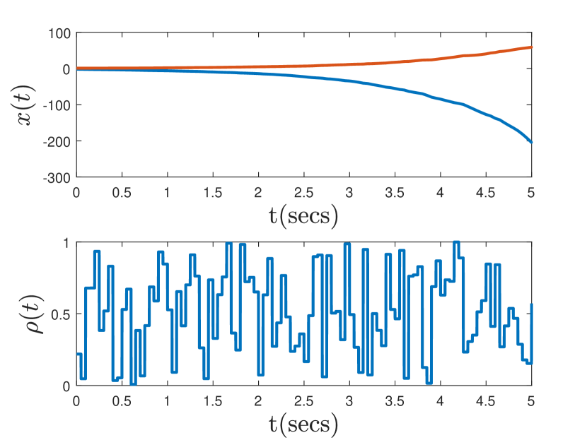
Figure 1: State trajectories of the open-loop system (top) and a typical parameter trajectory (bottom)

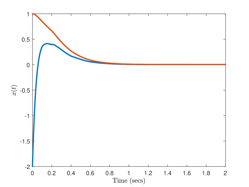
Figure 2: State trajectories of the closed-loop system under a step disturbance

4.3 Example 3: Consensus problem of multi-agent systems

In this example, we illustrate the application of our results to consensus problem of a multi-agent nonholonomic system subject to a switching topology.

Consider the following multi-agent system with six agents ($N=6$) considered in Gonzalez and Werner (2014):

$$\begin{array}[]{lll}\dot{\bar{x}}(t)&=&(I_{N}\otimes\mathcal{A})\bar{x}(t)+(\mathcal{L}(t)\otimes\mathcal{A}_{d})\bar{x}(t-d(t))\\ &&+(I_{N}\otimes\mathcal{B})\bar{u}(t)+(I_{N}\otimes\mathcal{E})\bar{w}(t)\\ \bar{z}(t)&=&(I_{N}\otimes\mathcal{C})\bar{x}(t)+(\mathcal{L}(t)\otimes\mathcal{C}_{d})\bar{x}(t-d(t))\\ &&+(I_{N}\otimes\mathcal{D})\bar{u}(t)+(I_{N}\otimes\mathcal{F})\bar{w}(t)\end{array}$$ (27)

where $\bar{x}(\theta)=\phi(\theta)$ for all $\theta\in\left[-h,0\right]$, $\bar{x}\in\mathbb{R}^{Nn}$, $\bar{u}\in\mathbb{R}^{Nq}$, $\bar{w}\in\mathbb{R}^{Nm}$, $\bar{z}\in\mathbb{R}^{Nr}$, and the system matrices are given by

$$\begin{array}[]{lll}\mathcal{A}=\left[\begin{matrix}0&1\\ -1&0\end{matrix}\right],\ \mathcal{A}_{d}=\left[\begin{matrix}0&1\\ -1&0\end{matrix}\right],\ \mathcal{B}=\left[\begin{matrix}1&0\\ 0&0.6\end{matrix}\right],\\ \mathcal{E}=0.05\times\mathcal{B},\ \mathcal{C}=\mathcal{C}_{d}=I_{2},\ \mathcal{D}=\mathcal{O}_{2},\ \mathcal{F}=0.1I_{2}\;.\end{array}$$ (28)

The upper bounds on delay and its derivative are chosen to be $h=0.2$ and $\mu=0.9$, respectively. For the system (27), we consider a switching topology represented by the following time-varying Laplacian matrix

$$\begin{array}[]{rcl}\mathcal{L}(t)=\sigma(t)\mathcal{L}_{1}+(1-\sigma(t))\mathcal{L}_{2}\;,\end{array}$$ (29)

where $\sigma(t)$ is a piecewise constant switching signal that takes value in $[0,1]$ with $T_{D}=0.1$, and $\mathcal{L}_{1},\mathcal{L}_{2}$ is a pair of symmetric commutable Laplacian matrices given by

$$\begin{array}[]{rcl}\mathcal{L}_{1}&=&\left[\begin{matrix}1&-0.5&0&0&0&-0.5\\ -0.5&1&-0.5&0&0&0\\ 0&-0.5&1&-0.5&0&0\\ 0&0&-0.5&1&-0.5&0\\ 0&0&0&-0.5&1&-0.5\\ -0.5&0&0&0&-0.5&1\\ \end{matrix}\right],\end{array}$$ (30)

$$\begin{array}[]{rcl}\mathcal{L}_{2}&=&\left[\begin{matrix}1&-0.25&-0.25&0&-0.25&-0.25\\ -0.25&1&-0.25&-0.25&0&-0.25\\ -0.25&-0.25&1&-0.25&-0.25&0\\ 0&-0.25&-0.25&1&-0.25&-0.25\\ -0.25&0&-0.25&-0.25&1&-0.25\\ -0.25&-0.25&0&-0.25&-0.25&1\\ \end{matrix}\right].\end{array}$$ (31)

For the matrices $\mathcal{L}_{1}$ and $\mathcal{L}_{2}$, the maximum and minimum eigenvalues are $\min\{\underline{\lambda}_{1},\ \underline{\lambda}_{2}\}=0$, $\max\{\bar{\lambda}_{1},\ \bar{\lambda}_{2}\}=2$, respectively. By defining a new piecewise constant parameter $\rho\in\mathscr{P}_{\geq T_{D}}$ with $\mathcal{P}=[0,\ \bar{\rho}]$ where $\bar{\rho}=2$ and using an approach similar to Corollary 2 of Zakwan and Ahmed (2020b), the distributed system (27) can be modeled as following LPV system with piecewise constant parameter:

$$\begin{array}[]{lll}\dot{x}(t)&=&A(\rho)x(t)+A_{d}(\rho)x(t-d(t))+B(\rho)u(t)+E(\rho)w(t)\\ z(t)&=&C(\rho)x(t)+C_{d}(\rho)x(t-d(t))+D(\rho)u(t)+F(\rho)w(t)\\ x(\theta)&=&\phi(\theta),\ \forall\theta\in\left[-h,0\right]\end{array}$$ (32)

where ${A}(\rho)=\mathcal{A}$, ${A}_{d}(\rho)=\rho\mathcal{A}_{d}$, $B(\rho)=\mathcal{B}$, $E(\rho)=\mathcal{E}$, ${C}(\rho)=C$, $C_{d}(\rho)=\rho\mathcal{C}_{d}$, $D(\rho)=\mathcal{D}$, and $F(\rho)=\mathcal{F}$.

Our goal is to design a clock-dependent distributed controller $\mathcal{K}(\tau,t)=I_{N}\otimes\mathcal{K}_{a}(\tau)+\mathcal{L}(t)\otimes\mathcal{K}_{b}(\tau)$. Using an approach similar to Corollary 2 of Zakwan and Ahmed (2020b), the distributed controller $\mathcal{K}(t)$ can be modelled as the clock-dependent gain-scheduled controller $\Sigma_{c}$ with gain ${K}(\tau,\rho)=K_{a}(\tau)+\rho K_{b}(\tau)$. We Choose $\kappa=0.01$ and then solve the LMIs in Theorem 2 using gridding approach with fifty points in YALMIP, Löfberg (2004). Note that to inherit same parametrization for controller as of the plant, we used $\tilde{U}(\tau,\rho)=\tau\tilde{U}_{a}+\rho\tilde{U}_{b}$. Once LMIs are feasible, we compute the matrix-valued function $\tilde{U}(\tau,\rho)$ which results in the following controller gains

$$\begin{array}[]{lll}K_{a}(\tau)=\left[\begin{matrix}-11.102\tau&-11.573\tau\\ 17.813\tau&-14.79\tau\end{matrix}\right]\\ K_{b}(\tau)=\left[\begin{matrix}-0.5078&-0.63061\\ 0.87181&-0.78384\end{matrix}\right]\;.\end{array}$$ (33)

The distributed controller gain $\mathcal{K}(t)$ can be constructed from $\mathcal{K}_{a}(\tau)=K_{a}(\tau)$ and $\mathcal{K}_{b}(\tau)=K_{b}(\tau)$.

We simulate the closed-loop system with a time-varying delay $\tau(t)=0.09sin(0.9t)+0.1$ under a unit-step disturbance. Fig. 3 shows the evolution of the state trajectories reaching a consensus subject to a typical switching signal shown in Fig. 4. For the random parameter trajectory shown in Fig. 4, the time between two successive jumps is taken equal to $T_{D}=0.1$ and the next value for the parameter is simply drawn from $\mathcal{U}(0,1)$. The consensus of multiagent system depicted in Fig. 3 under a switching topology and time-varying delay reflects the efficacy of the approach.

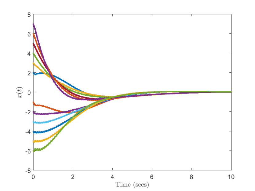
Figure 3: State trajectories of the closed-loop system under a step disturbance

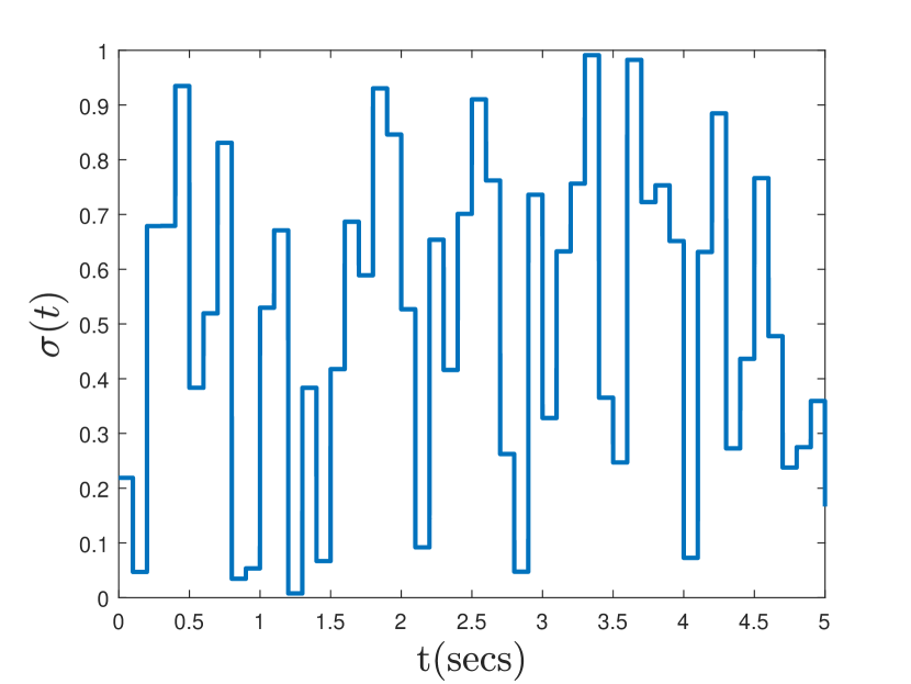
Figure 4: A typical realization of the piecewise constant switching signal $\sigma(t)$

5 Concluding Remarks

Dwell-time based stability conditions and synthesis conditions for gain-scheduled $\mathcal{L}_{2}$ state-feedback controllers are derived for a class of LPV systems with piecewise parameters under time-varying delay. One of the main advantages of our approach is reduced conservatism with improved performance as compared to more generalized methods such as quadratic stability.

Several extensions of this work are possible; for instance, dynamic $\mathcal{L}_{2}$ output feedback control, improving the bound on the rate of change of time delay, considering stochastic time-delays and stochastic piecewise constant parameter trajectories.

The authors would like to thank Dr. Corentin Briat for his useful suggestions to improve the quality of this paper.

References

• (1)
• Ahmed et al. (2018) Ahmed, S., Frédéric Mazenc and Hitay Özbay (2018). Dynamic output feedback stabilization of switched linear systems with delay via a trajectory based approach. Automatica 93, 92–97.
• Briat (2013) Briat, C. (2013). Convex conditions for robust stability analysis and stabilization of linear aperiodic impulsive and sampled-data systems under dwell-time constraints. Automatica 49(11), 3449–3457.
• Briat (2015a) Briat, C. (2015a). Linear Parameter-Varying and Time-Delay Systems – Analysis, Observation, Filtering & Control. Springer-Verlag, Berlin-Heidelberg.
• Briat (2015b) Briat, C. (2015b). Stability analysis and control of a class of LPV systems with piecewise constant parameters. Systems & Control Letters 82, 10–17.
• Briat (2018) Briat, C. (2018). Stability analysis and state-feedback control of LPV systems with piecewise constant parameters subject to spontaneous poissonian jumps. IEEE Control Systems Letters 2(2), 230 – 235.
• Briat et al. (2010) Briat, C., Olivier Sename and Jean-François Lafay (2010). Memory-resilient gain-scheduled state-feedback control of uncertain LTI/LPV systems with time-varying delays. Systems & Control Letters 59(8), 451–459.
• Chiasson and Loiseau (2007) Chiasson, J. and Jean Jacques Loiseau (2007). Applications of Time Delay Systems. Springer-Verlag, Berlin-Heidelberg.
• Gahinet and Apkarian (1994) Gahinet, P. and Pierre Apkarian (1994). A linear matrix inequality approach to ${H_{\infty}}$ control. International Journal of Robust and Nonlinear Control 4(4), 421–448.
• Gilbert et al. (2010) Gilbert, W., Didier Henrion, Jacques Bernussou and David Boyer (2010). Polynomial LPV synthesis applied to turbofan engines. Control Engineering Practice 18(9), 1077–1083.
• Gonzalez and Werner (2014) Gonzalez, A. M. and Herbert Werner (2014). LPV formation control of non-holonomic multi-agent systems. IFAC Proceedings Volumes 47(3), 1997–2002.
• Gu et al. (2003) Gu, K., Vladimir L Kharitonov and Jie Chen (2003). Stability of Time-Delay Systems. Birkhäuser, Basel.
• Joo and Kim (2015) Joo, H. and Sung Hyun Kim (2015). LPV control with pole placement constraints for synchronous buck converters with piecewise-constant loads. Mathematical Problems in Engineering, vol. 2015, Article ID 686857, 8 pages.
• Kajiwara et al. (1999) Kajiwara, H., Pierre Apkarian and Pascal Gahinet (1999). LPV techniques for control of an inverted pendulum. IEEE Control Systems Magazine 19(1), 44–54.
• Löfberg (2004) Löfberg, J. (2004). YALMIP: A toolbox for modeling and optimization in MATLAB. In Proceedings of the IEEE International Symposium on Computer Aided Control Systems Design. New Orleans, LA, USA. pp. 284–289.
• Mohammadpour and Scherer (2012) Mohammadpour, J. and Carsten W Scherer (2012). Control of Linear Parameter Varying Systems with Applications. Springer-Verlag, New York.
• Niculescu (2001) Niculescu, S.-I. (2001). Delay Effects on Stability: A Robust Control Approach. Springer-Verlag, London.
• Pang and Zhang (2015) Pang, G.-C. and Kan-Jian Zhang (2015). Stability of time-delay system with time-varying uncertainties via homogeneous polynomial Lyapunov-Krasovskii functions. International Journal of Automation and Computing 12(6), 657–663.
• Scherer and Hol (2006) Scherer, C. W. and Camile WJ Hol (2006). Matrix sum-of-squares relaxations for robust semi-definite programs. Mathematical programming 107(1-2), 189–211.
• Sename et al. (2013) Sename, O., Peter Gaspar and József Bokor (2013). Robust Control and Linear Parameter Varying Approaches: Application to Vehicle Dynamics. Springer-Verlag, Berlin-Heidelberg.
• Shin et al. (2000) Shin, J.-Y., Gary J Balas and Andrew K Packard (2000). $\mathcal{H}_{\infty}$ control of the V132 X-38 lateral-directional axis. In Proceedings of the American Control Conference. Chicago, IL, USA. pp. 1862–1866.
• Tan et al. (2002) Tan, K., Karolos M Grigoriadis and Fen Wu (2002). Output-feedback control of LPV sampled-data systems. International Journal of Control 75(4), 252–264.
• T´oth (2010) T´oth, R. (2010). Modeling and Identification of Linear Parameter-Varying Systems. Springer-Verlag, Berlin-Heidelberg.
• Wu and Prajna (2005) Wu, F. and S Prajna (2005). SOS-based solution approach to polynomial LPV system analysis and synthesis problems. International Journal of Control 78(8), 600–611.
• Zakwan (2020) Zakwan, M. (2020). Dynamic $L_{\text{2}}$ output feedback stabilization of LPV systems with piecewise constant parameters subject to spontaneous poissonian jumps. IEEE Control Systems Letters 4(2), 408–413.
• Zakwan and Ahmed (2020a) Zakwan, M. and Saeed Ahmed (2020a). Distributed output feedback control of decomposable LPV systems with delay and switching topology: Application to consensus problem in multi-agent systems. International Journal of Control. doi:10.1080/00207179.2019.1710257.
• Zakwan and Ahmed (2020b) Zakwan, M. and Saeed Ahmed (2020b). On output feedback stabilization of time-varying decomposable systems with switching topology and delay. In 21st IFAC World Congress. Berlin, Germany. arXiv:2001.01593v1 [eess.SY].