Integrable Field Theories with an Interacting Massless Sector

Abstract

We present the first known integrable relativistic field theories with interacting massive and massless sectors. And we demonstrate that knowledge of the massless sector is essential for understanding of the spectrum of the massive sector. Terms in this spectrum polynomial in the spatial volume (the accuracy for which the Bethe ansatz would suffice in a massive theory) require not just Lüscher-like corrections (usually exponentially small) but the full TBA integral equations. We are motivated by the implications of these ideas for AdS/CFT, but present here only field-theory results.

Introduction

Integrable quantum field theories are an important class of exactly solvable models. Many, like the $O(N)$ and sine-Gordon models (Hasenfratz:1990hq, ; Zamolodchikov:1995xk, ), contain massive excitations, whose asymptotic S-matrix is the basic ingredient for their solution. Some contain instead massless excitations, whose S-matrix plays the same role (Zamolodchikov:1991vx, ). Among models which contain both, or have adjustable mass parameters, it is generally believed that the massless sector decouples, and so the two sectors can be studied independently.

This paper studies some theories for which this decoupling does not occur. We find a double-scaling limit of certain Homogeneous Sine-Gordon (HSG) models (Park:1994bx, ; Hollowood:1994vx, ; FernandezPousa:1996hi, ), in which some of the particles become truly massless, yet retain a nontrivial interaction with the massive particles. And we show that the massless virtual particles must be included in the calculation of the spectrum of massive excitations. We discuss examples in which the full Thermodynamic Bethe Ansatz (TBA) (Yang:1966ty, ; Zamolodchikov:1989cf, ) is required, and one for which Lüscher terms (Luscher:1985dn, ) are sufficient.

Our main motivation for seeking out such theories comes from the AdS/CFT correspondence in string theory (Maldacena:1997re, ). In the planar limit, this is a complicated integrable model, and techniques of integrability have enabled the calculation of various quantities far beyond either weak- or strong-coupling perturbation theory (Beisert:2010jr, ). One version of this correspondence involves strings on $AdS_{3}\times S^{3}\times T^{4}$, where the presence of the flat torus $T^{4}$ introduces massless excitations into the (light-cone gauge) string theory (Babichenko:2009dk, ; Borsato:2014hja, ). Fully incorporating these into the integrable description is the principal challenge of adapting what we know about the $AdS_{5}\times S^{5}$ correspondence to this less-symmetric variant. The difficulties of doing so have left open various disagreements concerning the energy of massive physical states (Abbott:2015pps, ), and our hope is that this papers’s simpler examples may shed some light.

$\mathbf{su(3)_{2}}$ Model

Homogeneous Sine-Gordon (HSG) models are an integrable family generalising the complex sine-gordon model (Park:1994bx, ; Hollowood:1994vx, ; FernandezPousa:1996hi, ; Miramontes:1999hx, ; CastroAlvaredo:1999em, ; Dorey:2004qc, ; Bajnok:2015eng, ). We consider $su(3)_{k}$ models, all of which have three adjustable parameters: $m_{i}$ for $i=1,2$ control the masses of the particles, and $\sigma$ is a rapidity offset. The simplest model for which our double-scaling limit exists is the $su(3)_{2}$ model. Its S-matrix is diagonal, with $S^{ij}$ as follows:

$$S(\theta)=\begin{bmatrix}-1&\tanh\frac{1}{2}(\theta+\sigma-\frac{\mathrm{i}\pi}{2})\\ -\tanh\frac{1}{2}(\theta-\sigma-\frac{\mathrm{i}\pi}{2})&-1\end{bmatrix}.$$

The vacuum TBA of this model was studied by (CastroAlvaredo:1999em, ), and following (Dorey:1996re, ) we extend this to obtain excited-state TBA equations with physical particles of mass $m_{1}$ :

$$\epsilon_{1}(\theta) =m_{1}L\cosh\theta+\sum_{k}\pi\mathrm{i}-\int\frac{d\phi}{2\pi}\>K^{12}(\theta-\phi)L_{2}(\phi)$$

$$\epsilon_{2}(\phi) =m_{2}L\cosh\phi+\sum_{k}\log S^{21}(\phi-\hat{\theta}_{k}-\tfrac{\mathrm{i}\pi}{2})$$

$$\qquad-\smash{\int\frac{d\theta}{2\pi}}\>K^{21}(\phi-\theta)L_{1}(\theta)$$ (1)

where $L_{i}(\theta)\equiv\log\left[1+e^{-\epsilon_{i}(\theta)}\right]$, and the interaction kernel is nonzero only between particles of different mass:

$$K^{ij}(\theta) \equiv-\mathrm{i}\partial_{\theta}\log S^{ij}(\theta).$$

$$=\frac{1}{\cosh(\theta\pm\sigma)},\quad i,j={\textstyle{1,2\atop 2,1}}.$$

The rapidities $\hat{\theta}_{k}$ of the physical particles are fixed in terms of their mode numbers $\hat{n}_{k}\in\mathbb{Z}$ by

$$\epsilon_{1}(\hat{\theta}_{k}+\tfrac{\mathrm{i}\pi}{2})=2\pi\mathrm{i}(\hat{n}_{k}+\tfrac{1}{2}).$$ (2)

The purpose of solving these integral equations is to find the energy

$$E=\sum_{k}m_{1}\cosh\hat{\theta}_{k}-\smash{\sum_{i=1,2}\int\frac{d\theta}{2\pi}}\>m_{i}\cosh\theta\>L_{i}(\theta).$$ (3)

Dropping all the integrals will convert (2) into the Bethe Ansatz Equations (BAE), momentum quantisation conditions for otherwise free particles (Bethe:1931hc, ; Faddeev:1977rm, ). Here these are simply $e^{\mathrm{i}m_{1}\sinh\hat{\theta}_{k}^{\mathrm{BAE}}}=\prod_{k^{\prime}\neq k}(-1)$. This approximation is usually justified when $L$ is large, as we generically expect $\epsilon_{i}(\theta)$ to be large, and hence the factor $L_{i}(\theta)$ which appears in every integral to be small. For a massive theory, it gives the energy to polynomial accuracy, i.e. including all terms in $1/L$.

The first corrections for smaller $L$ are the Lüscher terms (Luscher:1983rk, ). In deriving these from the TBA there are two contributions (Bajnok:2008bm, ): $\delta E_{\mathrm{int}}$ is the integrals in energy (3), and

$$\delta E_{\mathrm{quant}}\equiv{\textstyle\sum_{k}}m_{1}\cosh\hat{\theta}_{k}-{\textstyle\sum_{k}}m_{1}\cosh\hat{\theta}_{k}^{\mathrm{BAE}}$$

comes from the integral in (1) via the quantisation condition (2). Both enter with a factor $e^{-m_{i}L}$, which ensures that the wrapping effect of a massive particle is exponentially suppressed; this may be thought of as a tunneling effect. Terms with $e^{-2m_{i}L}$ are called double-wrapping effects.

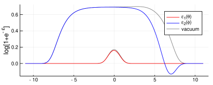
Figure 1: A solution of the $su(3)_{2}$ model (1), with $m_{1}=1$, $m_{2}=10^{-3}$ and $\sigma=4$, in length $L=2$. The vacuum solution is shown in gray, while the coloured lines are an excited state with $\hat{n}_{k}=1$ hence $\hat{\theta}_{1}=2.238$. We are interested in much larger $L$, for which the red line $L_{1}(\theta)\sim e^{-m_{1}L}\to 0$, and even smaller $m_{2}$ such that $m_{2}L\to 0$. Then the blue line $L_{2}(\phi)$ is order 1 for $\left|\phi\right|\lesssim-\log m_{2}L\to\infty$.

However, Lüscher terms arising from massless virtual particles need not be so suppressed. Their exponent contains $m_{2}L\cosh\phi$ which approaches $L\left|p\right|$ in the limit $m_{2}\to 0$, giving polynomial corrections like $\int dp\>e^{-L\left|p\right|}=2/L$. It is the momentum $p=m_{2}\sinh\phi$ which is well-defined in the massless limit, while $\phi$ diverges. Figure 1 shows a comparison between massive $L_{1}(\theta)$ and near-massless $L_{2}(\phi)$.

In many theories this divergence of rapidity $\phi$ would cause the interaction $S^{12}$ to become trivial. But in HSG models it is possible to compensate with the shift parameter $\sigma$, and so we propose taking this double-scaling limit:

$$m_{2}\to 0,\quad\sigma\to+\infty,\quad\sigma_{0}=\sigma+\log(m_{2}/2)\sim 1.$$ (4)

Our choice of the sign of $\sigma$ means that it is the right-moving particles which retain an interaction:

$$S^{21}(\phi-\hat{\theta}_{k}-\tfrac{\mathrm{i}\pi}{2})\to\begin{cases}-1\big{/}\tanh\frac{\log p-\hat{\theta}_{k}-\sigma_{0}}{2},&p>0\\ +1&p<0.\end{cases}$$

Dropping all order $e^{-m_{1}L}$ pieces, the integral in (3) arising from massless virtual particles then reads

$$\negthickspace\delta E_{\mathrm{int}}\negthickspace =\frac{-\pi}{24L}-\negthickspace\int_{0}^{\infty}\negthickspace\frac{dp}{2\pi}\log\Big{[}1-e^{-L|p|}\prod_{k}\tanh\tfrac{\log p-\hat{\theta}_{k}-\sigma_{0}}{2}\Big{]}$$

$$=\frac{\pi}{12}\Big{[}-\frac{1}{L}+\frac{1}{L^{2}}-\frac{2+c_{1}}{L^{3}}+\mathcal{O}\Big{(}\frac{1}{L^{4}}\Big{)}\Big{]}$$ (5)

at $\sigma_{0}=0$, for one particle at $\hat{\theta}_{1}=c_{1}/L+c_{2}/L^{2}+\ldots$. This expansion can be checked against a numerical solution of the full TBA (1) at small but finite $m_{2}=10^{-6}$, and we see perfect agreement. Analytically, notice that if we expand in the wrapping number (i.e. in $e^{-L\left|p\right|}$) then every wrapping contributes at order $1/L$. However, expanding the integrand in $1/L$, holding fixed $y=pL$, gives the series shown.

The quantisation condition (2) can be treated in the same way. The effect of massless virtual particles enters $\hat{\theta}_{k}$ at order $1/L^{2}$, and hence affects the energy as $\delta E_{\mathrm{quant}}\propto c_{2}/L^{3}$.

$\mathbf{su(3)_{3}}$ Model

What the above $su(3)_{2}$ example lacks is interactions between the massless particles. We next turn to the $su(3)_{3}$ HSG model, which has the same three parameters $m_{1}$, $m_{2}$, $\sigma$ but now two particles of each mass, $a,b=1,2$. (It also has a discrete parameter, a 3rd root of $-1$, which we take to be $\eta=-1$ for simplicity.) The S-matrix is again diagonal, and we write $S_{ab}^{ij}(\theta_{a,i}-\theta_{b,j})$ for a particle of mass $m_{i}$ and label $a$ scattering with one of $m_{j},b$. This is

$$S^{ij}(\theta)\,= \delta_{ij}\,\begin{bmatrix}(2)_{\theta}&-(1)_{\theta}\\ -(1)_{\theta}&(2)_{\theta}\end{bmatrix}$$

$$+\bigl{(}1-\delta_{ij}\bigr{)}\,\begin{bmatrix}-(-1)_{\theta+\sigma_{ij}}&(-2)_{\theta+\sigma_{ij}}\\ (-2)_{\theta+\sigma_{ij}}&-(-1)_{\theta+\sigma_{ij}}\end{bmatrix}$$

where $\sigma_{12}=-\sigma_{21}=\sigma$ and

$$(n)_{\theta}\equiv\sinh\tfrac{1}{2}(\theta+\tfrac{\mathrm{i}\pi}{3}n)/\sinh\tfrac{1}{2}(\theta-\tfrac{\mathrm{i}\pi}{3}n).$$

The complete TBA has four pseudo-energies $\epsilon_{a,i}(\theta)$, and we again consider an excited-state TBA with physical particles of mass $m_{1}$, and label $a=1$. This reads

$$\epsilon_{a,i}(\theta)\,= m_{i}L\cosh\theta+\sum_{k}\log S_{a1}^{i1}(\theta-\hat{\theta}_{k}-\tfrac{\mathrm{i}\pi}{2})$$

$$-\smash{\sum_{b,j}\int\frac{d\theta^{\prime}}{2\pi}}\;K_{ab}^{ij}(\theta-\theta^{\prime})L_{b,j}(\theta^{\prime})$$ (6)

with energy

$$E =\sum_{k}m_{1}\cosh\hat{\theta}_{k}-\sum_{b,j}\int\frac{d\theta}{2\pi}\>m_{j}\cosh\theta\>L_{b,j}(\theta).$$ (7)

The quantisation condition for $\hat{\theta}_{k}$ is now $\epsilon_{1,1}(\hat{\theta}_{k}+\tfrac{\mathrm{i}\pi}{2})=2\pi\mathrm{i}(\hat{n}_{k}+\tfrac{1}{2})$, which in the large-$L$ limit gives us the following Bethe equations:

$$e^{\mathrm{i}m_{1}L\sinh\hat{\theta}_{j}^{\mathrm{BAE}}}{\textstyle\prod_{k}}\>S_{11}^{11}(\hat{\theta}_{j}^{\mathrm{BAE}},\hat{\theta}_{k}^{\mathrm{BAE}})=-1.$$

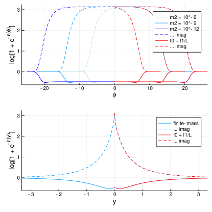
Figure 2: Pseudo-energy $\epsilon_{1,2}(\phi)$ for the $su(3)_{3}$ HSG model, showing the solution to (8) in length $L=10^{3}$ with masses $m_{2}=10^{-6},10^{-9},10^{-12}$ (in blue), and on the same axes as the zero-mass $f_{n}(y)$ expansion (12) (drawn for $y>0$ only, in red). As a function of $\phi$ (above) the range for which $L_{1,2}(\phi)$ is order 1 grows as the mass $m_{2}$ is decreased. As a function of $y=m_{2}L\sinh\phi$ (below) the massless limit is well-behaved. We use mode number $\hat{n}_{k}=1$ hence $\hat{\theta}_{1}=4\pi/L+\ldots$, mass $m_{1}=1$, shift $\sigma=-\log m_{2}/2$. Solid lines are the real parts, dashed lines imaginary.

Massless TBA

To study the TBA in the $m_{2}\to 0$ limit, we now fix $m_{1}\approx 1$ and drop all exponentially small terms, that is, all integrals containing $L_{a,1}(\theta)$ above. Because we have only physical particles of type $a=i=1$, the two massless equations are complex conjugates, $\epsilon_{2,2}(\phi)=\overline{\epsilon_{1,2}}(\phi)$, leaving just one integral equation:

$$\epsilon_{1,2}(\phi)=m_{2}L\cosh\phi-{\textstyle\sum_{k}}\log s(\phi-\hat{\theta}_{k}-\sigma)+\mathrm{i}\pi$$ (8)

$$+\sqrt{3}\int\frac{d\phi^{\prime}}{2\pi}\left[\frac{L_{1,2}(\phi^{\prime})}{1+2\cosh(\phi-\phi^{\prime})}-\frac{\overline{L_{1,2}}(\phi^{\prime})}{1-2\cosh(\phi-\phi^{\prime})}\right]$$

where $s(\theta)\equiv(1)_{\theta-\frac{\mathrm{i}\pi}{2}}=\sinh(\tfrac{\theta}{2}-\tfrac{\mathrm{i}\pi}{12})/\sinh(\tfrac{\theta}{2}-\tfrac{\mathrm{i}5\pi}{12})$, and

$$E=\sum_{k}m_{1}\cosh\hat{\theta}_{k}-\int\frac{d\phi}{2\pi}m_{2}\cosh\phi\left[L_{1,2}(\phi)+\overline{L_{1,2}}(\phi)\right].$$

We can solve this numerically at small finite $m_{2}$, but can also take a strict $m_{2}\to 0$ limit analytically, using the same double-scaling limit as above, (4). It is again the mixed-mass S-matrix elements which contain the shift $\sigma$, and choosing to take $\sigma\to+\infty$ keeps the coupling to right-moving massless modes nontrivial:

$$s(\phi-\hat{\theta}_{k}-\sigma)\to s_{+}(p,\hat{\theta}_{k})\equiv\begin{cases}s(\log p-\hat{\theta}_{k}-\sigma_{0}),&p>0\\ e^{-\mathrm{i}\pi/3}&p<0.\end{cases}$$

Notice that in this limit, where $\left|\phi\right|,\left|\phi^{\prime}\right|\to\infty,$ the denominators of (8) diverge unless $\phi$ and $\phi^{\prime}$ have the same sign. Hence the integral equation for $\epsilon(p),p>0$ is decoupled from that for $p<0$:

$$\epsilon_{1,2}(p)=L\left|p\right|-{\textstyle\sum_{k}}\log s_{+}(p,\hat{\theta}_{k})+\mathrm{i}\pi$$ (9)

$$+\frac{\sqrt{3}}{2\pi}\int_{0}^{\infty}\frac{dp^{\prime}}{p^{\prime}}\left[\frac{L_{1,2}(\pm p^{\prime})}{1+\frac{\left|p\right|}{p^{\prime}}+\frac{p^{\prime}}{\left|p\right|}}-\frac{\overline{L_{1,2}}(\pm p^{\prime})}{1-\frac{\left|p\right|}{p^{\prime}}-\frac{p^{\prime}}{\left|p\right|}}\right],\;p\gtrless 0.$$

The energy contains $\delta E_{\mathrm{int}}=-\int\frac{dp}{2\pi}\left[L_{1,2}(p)+\mathrm{c.c.}\right]$, notice the different measure. And the quantisation condition (for one physical particle, $\hat{\theta}_{1}\in\mathbb{R}$) reads

$$2\pi\mathrm{i}\hat{n}_{k} =\mathrm{i}m_{1}L\sinh\hat{\theta}_{1}-2\pi\mathrm{i}$$ (10)

$$+\frac{\sqrt{3}}{2\pi}\int_{0}^{\infty}\frac{dp}{p}\left[\frac{\log(1+e^{-\epsilon_{1,2}(p)})}{1-2\mathrm{i}\sinh(\hat{\theta}_{1}-\log p+\sigma_{0})}-\mathrm{c.c.}\right].$$

This limit eliminates $m_{2}$ but not $L$ from the integral equation. To find large-$L$ solutions, we claim that you should expand in $1/L$ holding fixed $pL$, the same small-momentum limit we used for (5) above:

$$\epsilon_{1,2}(p) =f_{0}(y)+\frac{f_{1}(y)}{L}+\frac{f_{2}(y)}{L^{2}}+\mathcal{O}\Big{(}\frac{1}{L^{3}}\Big{)}$$ (11)

$$\hat{\theta}_{1} =c_{1}/L+c_{2}/L^{2}+\ldots,\qquad y=pL.$$

This ansatz gives an integral equation at each power of $1/L$. For $y<0$, clearly (9) is independent of $L$, hence only $f_{0}(y)$ is nonzero there. The first few equations are:

$$f_{0}(y) =\left|y\right|+2\pi\Big{(}1-\frac{\mathop{\mathrm{sign}}(y)}{3}\Big{)}+\frac{\sqrt{3}}{2\pi}\int_{0}^{\infty}\frac{dy^{\prime}}{y^{\prime}}\Bigg{[}\frac{\log(1+e^{-f_{0}(\pm y^{\prime})})}{1+\frac{\left|y\right|}{y^{\prime}}+\frac{y^{\prime}}{\left|y\right|}}-\frac{\log(1+e^{-\overline{f_{0}}(\pm y^{\prime})})}{1-\frac{\left|y\right|}{y^{\prime}}-\frac{y^{\prime}}{\left|y\right|}}\Bigg{]},\negthickspace\negthickspace\negthickspace \negthickspace\negthickspace\negthickspace y \gtrless 0$$ (12)

$$f_{1}(y) =\frac{\sqrt{3}y}{2}-\frac{\sqrt{3}}{\pi}\int_{0}^{\infty}\frac{dy^{\prime}}{y^{\prime}}\Big{[}\frac{f_{1}(y^{\prime})}{(1+e^{+f_{0}(y^{\prime})})(1+\frac{y}{y^{\prime}}+\frac{y^{\prime}}{y})}-\frac{\bar{f_{1}}(y^{\prime})}{(1+e^{+\bar{f_{0}}(y^{\prime})})(1-\frac{y}{y^{\prime}}-\frac{y^{\prime}}{y})}\Big{]}, \negthickspace\negthickspace\negthickspace y >0$$

$$f_{2}(y) =\frac{-\mathrm{i}\sqrt{3}y^{2}}{2}-\sqrt{3}yc_{1}+\frac{\sqrt{3}}{4\pi}\int_{0}^{\infty}\frac{dy^{\prime}}{y^{\prime}}\Big{[}\frac{e^{+f_{0}(y^{\prime})}f_{1}(y^{\prime})-2(1+e^{+f_{0}(y^{\prime})})f_{2}(y^{\prime})}{(1+e^{+f_{0}(y^{\prime})})^{2}(1+\frac{y}{y^{\prime}}+\frac{y^{\prime}}{y})}-...\Big{]}, \negthickspace\negthickspace\negthickspace y >0.$$

These can be solved in sequence, as each depends only on lower-order functions $f_{n}(y)$, and lower-order coefficients $c_{n}$. The resulting pseudo-energy $\epsilon_{1,2}(\phi)$ is shown in Figure 2. On the same axes we show the result of solving (8) at small but finite $m_{2}$; see the appendix for a discussion of numerical issues here. The coefficients of $\hat{\theta}_{1}$ are found by expanding (10), and solving:

$$\negthickspace c_{1} =\frac{2\pi}{m_{1}}(\hat{n}_{k}+1) =4\pi$$ (13)

$$\negthickspace c_{2} =-\frac{\sqrt{3}}{m_{1}}\smash{\int}\frac{dy}{2\pi}\left[\log(1+e^{-f_{0}(y)})+\text{c.c.}\right] \approx 0.362$$

$$\negthickspace\negthickspace\negthickspace\negthickspace\negthickspace\negthickspace c_{3} \approx-336.6\,.$$

The same numerical solutions $f_{n}(y)$ give the values shown (for mode number $\hat{n}_{k}=1$, mass $m_{1}=1$, shift $\sigma_{0}=0$), and again these agree with the TBA at small finite $m_{2}$. These corrections to the quantisation condition for $\hat{\theta}_{1}$ are (through the $m_{1}\cos\hat{\theta}_{1}$ term) one source of corrections to the energy:

$$\delta E_{\mathrm{quant}}=\frac{c_{1}c_{2}}{L^{3}}+\ldots\approx\frac{4.558}{L^{3}}+\mathcal{O}\Big{(}\frac{1}{L^{4}}\Big{)}.$$ (14)

The other source is the integral term in (7), which can be similarly expanded:

$$\delta E_{\mathrm{int}} =-\smash{\frac{1}{L}\int\frac{dy}{2\pi}}\left[\log(1+e^{-f_{0}(y)})+\text{c.c.}\right]$$

$$\qquad\qquad+\frac{1}{L^{2}}\int\frac{dy}{2\pi}\left[\frac{f_{1}(y)}{1+e^{f_{0}(y)}}+\text{c.c.}\right]+\ldots$$

$$\approx\frac{0.418}{L}-\frac{0.363}{L^{2}}+\frac{5.855}{L^{3}}+\mathcal{O}\Big{(}\frac{1}{L^{4}}\Big{)}.$$ (15)

We are able to check the first three terms here against the finite-$m_{2}$ numerical solution to (8), and Figure 3 shows the comparison.

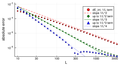
Figure 3: Comparison of the energy correction $\delta E_{\mathrm{int}}$ from the $m_{2}=0$ expansion (15), to that from solving the TBA (8) at $m_{2}=10^{-12}$. Including more terms (up to $1/L^{3}$) reduces the error, at moderately large $L$. (At around $L=300$ the error changes sign, and we run out of precision.)

For contrast, we can also find the Lüscher contribution here (instead of solving the integral equation) by dropping the integral in (9). The answer is very different:

$$\delta E_{\mathrm{int}} =-\int\frac{dp}{2\pi}\left[\log\big{(}1-e^{-\left|L\right|p}s_{+}(p,\hat{\theta}_{1})\big{)}+\mathrm{c.c.}\right]$$

$$\approx-\frac{0.349}{L}+\frac{0.302}{L^{2}}+\mathcal{O}\Big{(}\frac{1}{L^{3}}\Big{)}.$$ (16)

Conclusion

By studying these simple models, we have learned:

1. Interacting relativistic integrable theories containing both massive and massless particles exist .

2. The spectrum of massive excitations depends on the massless sector, including massless-massless interactions. Calculating this $E$ to polynomial accuracy in $L$, which in a massive theory requires only the BAE, now requires at least the massless-sector TBA.

3. Either left- or right-moving massless particles could be nontrivially coupled to the massive modes, but not both. We expect that more complicated theories can somewhat avoid this .

4. While an expansion in the wrapping order (i.e. in $e^{-L\left|p\right|}$) is no longer meaningful, the energy calculation can be organised as a series in $1/L$ by expanding at small momentum, holding $pL$ fixed.

As mentioned above, our motivation for this work comes from string integrability in the AdS/CFT correspondence. The light-cone gauge string is viewed as a non-relativistic integrable field theory, living on the worldsheet whose spatial extent $L$ is proportional to an angular momentum $J$. And in $AdS_{3}\times S^{3}\times T^{4}$ this theory has massless excitations.

In earlier work (Abbott:2015pps, ), we showed that some disagreements in the one-loop spectrum of the massive sector $AdS_{3}\times S^{3}$ appear to be caused by interactions with the massless sector. In particular, we were able to calculate massless Lüscher corrections for circular spinning strings, for which there was a long-standing mismatch. We included all orders of wrappings following (Heller:2008at, ), and treated the multi-particle physical state following (Bajnok:2008bm, ), to calculate :

$$\delta E=\sum_{b}^{4+4}(-1)^{F_{b}}\negthickspace\int\negthickspace d\phi\sum_{n=1}^{\infty}\frac{1}{n}e^{-nLm_{2}\cosh\phi}\prod_{k}^{\negthickspace\negthickspace\mathcal{O}(\sqrt{\lambda})\negthickspace\negthickspace}S_{b1}(\phi-\hat{\theta}_{k})^{n}.$$

This formula allowed us to correct the mismatch between BAE and string theory calculations (up to a factor of 2) for strings moving in $S^{3}$, called the $su(2)$ sector. However, there are comparable mismatches for other solutions, such as $sl(2)$-sector circular strings, for which a similar calculation does not succeed. This formula is the analogue of (5) or (16) here. What we add now is the first glimpse of the world beyond these wrapping corrections: the interactions of massless modes with each other lead to different results.

Since our paper (Abbott:2015pps, ), there has been some work on the massless TBA (Bombardelli:2018jkj, ; Fontanella:2019ury, ). Unlike the massive sector, there appear to be no complications with massless bound states. These papers take a small-$p$ limit in which the system becomes relativistic. However they do not yet incorporate massive-massless interactions, which are essential for the effects on the massive spectrum studied here. It would be very interesting to find ways to remedy this.

Numerical Methods

We solve all of these integral equations iteratively, starting with $\epsilon(\phi)=0$ and then at time step $t$ replacing

$$\epsilon(\phi):=\lambda^{t}\mathop{\mathrm{rhs}}[\epsilon](\phi)+(1-\lambda^{t})\epsilon(\phi).$$

Here $\lambda=0.99$ controls how fast the updates decay. Some such damping is essential in order to find stable and accurate solutions. The function $\epsilon(\phi)$ is encoded either as a sum of Chebyshev polynomials, or just values at a grid of points $\phi_{i}$.

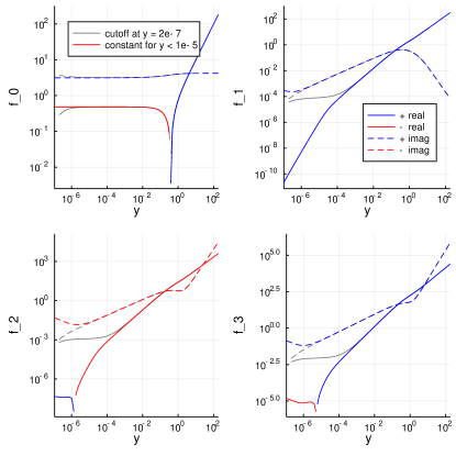
Figure 4: Terms $f_{n}(y)$ of the expansion (11). The lines in colour use $f_{0}(y)=-0.48+\mathrm{i}\pi$ for $y<10^{-5}$, while the lines in gray do not, and hence suffer more strongly from boundary effects. Dashed lines indicate the imaginary part, and red indicates negative values.

The equations (12) for $f_{n}(y)$ deserve extra comment. We use a grid of points evenly spaced in $\phi$, which necessarily has some smallest value $y_{\mathrm{min}}$. The integration measure $\int dy^{\prime}/y^{\prime}$ is uniform in $\log y$ and thus arbitrarily small $y^{\prime}$ are weighted equally. In particular, the values $y^{\prime}<y_{\mathrm{min}}$ which we omit would appear inside the integral needed for $f_{n}(y>y_{\mathrm{min}})$. This effect is of finite range in $\log y$, thanks to factors $1/[1\pm 2\cosh(\log y-\log y^{\prime})]$ in the integrand, and thus we believe it contaminates a only the end of the range of values considered.

Figure 4 shows these boundary effects. With a cutoff $y_{\mathrm{min}}=2\times 10^{-7}$, values of $f_{0}(y)$ for $y<10^{-6}$ deviate, but it is simple to correct this by solving the small-$y$ limit directly:

$$f_{0}(0) =\frac{4\mathrm{i}\pi}{3}+I_{+}\log(1+e^{-f_{0}(0)})-I_{-}\log(1+e^{-\bar{f_{0}}(0)})$$

$$\approx-0.48+\mathrm{i}\pi$$

where $I_{\pm}\equiv\frac{\sqrt{3}}{2\pi}\int_{0}^{\infty}\frac{dy}{y}\frac{1}{1\pm(y+1/y)}$ with no cutoff. Fixing $f_{0}(y)$ to be exactly this for $y<10^{-5}$ obviously produces a perfectly straight line in both Figure 4 and Figure 2. The other $f_{n}(y)$ have similar boundary effects which are not so easily removed, but the effect of clamping $f_{0}(y)$ to a constant is the difference between the gray and coloured curves in Figure 4.

The energy integrals (15), which are the motivation for finding functions $f_{n}(y)$, have a different integration measure, simply $\int dy$. Thus very small $y$ values contribute vanishingly little to $\delta E_{2}$. The digits shown for $\delta E_{2}$ in (15) above are unchanged by clamping $f_{0}(y)$ to a constant like this, and also unchanged by only integrating over $y>10^{-3}$.

The numerical solution also needs a cutoff $y_{\mathrm{max}}$. Here there are no awkward issues, as the integrand always has a factor $e^{-f_{0}(y)}$ which rapidly kills it. This is true for both $f_{n}(y)$ integral equations (12), and for the energy integrals (15).

Finally, in the text we claim agreement between the coefficients $c_{n}$ found along with these $f_{n}(y)$, shown in (13), and the result of solving the TBA (8) at small but finite $m_{2}$. Figure 5 shows some data on this.

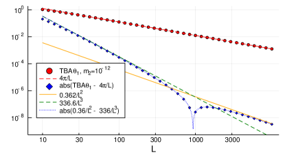
Figure 5: Comparison of $\hat{\theta}_{1}$ from solving (8) at $m_{2}=10^{-12}$, to the expansion $c_{1}/L+c_{2}/L^{2}+c_{3}/L^{3}+\ldots$, using the first three $c_{n}$ as shown in (13). The difference $\hat{\theta}_{1}-4\pi/L$ changes sign around $L=1000$, causing a dip in the blue points.

References

- (1) P. Hasenfratz, M. Maggiore and F. Niedermayer, The exact mass gap of the O(3) and O(4) non-linear -models in d = 2, Physics Letters B 245 (1990) 522–528.
- (2) A. B. Zamolodchikov, Mass scale in the sine-Gordon model and its reductions, Int. J. Mod. Phys. A10 (1995) 1125–1150.
- (3) A. B. Zamolodchikov, From tricritical Ising to critical Ising by thermodynamic Bethe ansatz, Nucl. Phys. B358 (1991) 524–546.
- (4) Q.-H. Park, Deformed coset models from gauged WZW actions, Phys. Lett. B328 (1994) 329–336 [arXiv:hep-th/9402038].
- (5) T. J. Hollowood, J. L. Miramontes and Q.-H. Park, Massive integrable soliton theories, Nucl. Phys. B445 (1995) 451–468 [arXiv:hep-th/9412062].
- (6) C. R. Fernandez-Pousa, M. V. Gallas, T. J. Hollowood and J. L. Miramontes, The Symmetric space and homogeneous sine-Gordon theories, Nucl. Phys. B484 (1997) 609–630 [arXiv:hep-th/9606032].
- (7) C. N. Yang and C. P. Yang, One-dimensional chain of anisotropic spin spin interactions. 1. Proof of Bethe’s hypothesis for ground state in a finite system, Phys. Rev. 150 (1966) 321–327.
- (8) A. B. Zamolodchikov, Thermodynamic Bethe Ansatz in Relativistic Models. Scaling Three State Potts and Lee-yang Models, Nucl. Phys. B342 (1990) 695–720.
- (9) M. Luscher, Volume Dependence of the Energy Spectrum in Massive Quantum Field Theories. 1. Stable Particle States, Commun. Math. Phys. 104 (1986) 177.
- (10) J. M. Maldacena, The large N limit of superconformal field theories and supergravity, Adv. Theor. Math. Phys. 2 (1998) 231–252 [arXiv:hep-th/9711200].
- (11) N. Beisert et. al., Review of AdS/CFT Integrability: An Overview, Lett. Math. Phys. 99 (2012) 3–32 [arXiv:1012.3982].
- (12) A. Babichenko, B. Stefanski and K. Zarembo, Integrability and the AdS3/CFT2 correspondence, JHEP 03 (2010) 058 [arXiv:0912.1723].
- (13) R. Borsato, O. Ohlsson Sax, A. Sfondrini and B. Stefanski, The complete AdS3 x S3 x T4 worldsheet S-matrix, JHEP 10 (2014) 066 [arXiv:1406.0453].
- (14) M. C. Abbott and I. Aniceto, Massless Luscher Terms and the Limitations of the AdS3 Asymptotic Bethe Ansatz, Phys. Rev. D93 (2016) 106006 [arXiv:1512.08761].
- (15) J. L. Miramontes and C. R. Fernandez-Pousa, Integrable quantum field theories with unstable particles, Phys. Lett. B472 (2000) 392–401 [arXiv:hep-th/9910218].
- (16) O. A. Castro-Alvaredo, A. Fring, C. Korff and J. L. Miramontes, Thermodynamic Bethe ansatz of the homogeneous Sine-Gordon models, Nucl. Phys. B575 (2000) 535–560 [arXiv:hep-th/9912196].
- (17) P. Dorey and J. L. Miramontes, Mass scales and crossover phenomena in the homogeneous sine-Gordon models, Nucl. Phys. B697 (2004) 405–461 [arXiv:hep-th/0405275].
- (18) Z. Bajnok, J. Balog, K. Ito, Y. Satoh and G. Z. Tóth, Exact mass-coupling relation for the homogeneous sine-Gordon model, Phys. Rev. Lett. 116 (2016) 181601 [arXiv:1512.04673].
- (19) P. Dorey and R. Tateo, Excited states by analytic continuation of TBA equations, Nucl. Phys. B482 (1996) 639–659 [arXiv:hep-th/9607167].
- (20) Our notation is that is a generic rapidity, and that of a physical excitation, . We write specifically for the rapidity of particles of mass , as we will take the limit .
- (21) H. Bethe, On the theory of metals. 1. Eigenvalues and eigenfunctions for the linear atomic chain, Z. Phys. 71 (1931) 205–226.
- (22) L. D. Faddeev and V. E. Korepin, Quantum Theory of Solitons: Preliminary Version, Phys. Rept. 42 (1978) 1–87.
- (23) M. Luscher, On a relation between finite size effects and elastic scattering processes, Cargese Summer Inst. (1983) 0451.
- (24) Z. Bajnok and R. A. Janik, Four-loop perturbative Konishi from strings and finite size effects for multiparticle states, Nucl. Phys. B807 (2009) 625–650 [arXiv:0807.0399].
- (25) We exclude here what are variously called pseudoparticles (Fendley:1992dm, ), auxiliary roots (Beisert:2005fw, ), or magnon Bethe roots (Gromov:2008gj, ). The massless excitations of interest are ordinary, propagating, momentum-carrying particles, on an equal footing with the massive ones.
- (26) For example the HSG models have three mass parameters for , and three independent shifts for , allowing (say) particles moving in either direction to remain coupled, but not coupled to the same massive species.
- (27) M. P. Heller, R. A. Janik and T. Lukowski, A new derivation of Luscher F-term and fluctuations around the giant magnon, JHEP 06 (2008) 036 [arXiv:0801.4463].
- (28) Here labels the 4 massless bosons and 4 massless fermions, and is the wrapping order. The physical solution is a condensate of a very large number, of order , of massive particles, all of the same type, which can be treated as a single cut in the complex plane (Hernandez:2006tk, ). The ’t Hooft coupling is in terms of the radius of the space, and plays the role of for these semiclassical strings.
- (29) D. Bombardelli, B. Stefanski and A. Torrielli, The low-energy limit of AdS3/CFT2 and its TBA, JHEP 10 (2018) 177 [arXiv:1807.07775].
- (30) A. Fontanella, O. Ohlsson Sax, B. Stefanski and A. Torrielli, The Effectiveness of Relativistic Invariance in AdS3, JHEP 07 (2019) 105 [arXiv:1905.00757].
- (31) P. Fendley and K. A. Intriligator, Scattering and thermodynamics in integrable N=2 theories, Nucl. Phys. B380 (1992) 265–290 [arXiv:hep-th/9202011].
- (32) N. Beisert and M. Staudacher, Long-range PSU(2,2|4) Bethe ansaetze for gauge theory and strings, Nucl. Phys. B727 (2005) 1–62 [arXiv:hep-th/0504190].
- (33) N. Gromov, V. Kazakov and P. Vieira, Finite Volume Spectrum of 2D Field Theories from Hirota Dynamics, JHEP 12 (2009) 060 [arXiv:0812.5091].
- (34) R. Hernandez and E. Lopez, Quantum corrections to the string Bethe ansatz, JHEP 07 (2006) 004 [arXiv:hep-th/0603204].