Accumulated densities of sedimenting particles in turbulent flows

Abstract

We study the effect of turbulence on a sedimenting layer of particles by means of direct numerical simulations. A Lagrangian model in which particles are considered as tracers with an additional downward settling velocity is integrated together with an isotropic homogeneous turbulent flow. We study the spatial distribution of particles when they are collected on a plane at non-asymptotic times. We relate the resulting coarse-grained particle density to the history of the stretching rate along the particle trajectory and the projection of the density onto the accumulation plane, and analyse the deviation from homogeneity in terms of the Reynolds number and the settling velocity. We identify two regimes that arise during the early and during the well-mixed stage of advection. In the former regime, more inhomogeneity in the particle distribution is introduced for decreasing settling velocity or increasing Reynolds number, while the tendencies are opposite in the latter regime. A resonant-like crossover is found between these two regimes, where inhomogeneity is maximal.

I Introduction

Sedimentation of particles in a turbulent flow is a crucial problem both for theory and applications. For example, it plays a key role in the process of rain formation in clouds falkovich2002 ; woittiez2009 . In the marine environment, sinking of particles is an important mechanism for many physical processes: in the sequestration of carbon dioxide delarocha2007 ; devries2012 , in the downward transport of organic and inorganic aggregates, such as marine snow alldredge1988 ; borgnino2019 , larval eggs and microplastics woodall2014 ; khatmullina2017 . Experimentally, a way to estimate the downward fluxes of particles in the ocean interior is performed by placing sediment traps siegel1997 ; buesseler2007 ; siegel2008 . An open question concerns the identification of the mechanisms that lead to the observed size and spatial distributions of particles which are collected at a given depth by the traps.

The interaction between particles and flow is determinant to establish the spatial distribution of particlesbalkovsky2001 . Advection of a homogeneous distribution of passive particles in an incompressible flow generally results in a homogeneous concentration of particles. Deviations from homogeneity may arise from some type of compressibility, either in the flow itself or in the motion of particles. In this case, particle dynamics is restricted to a lower-dimensional or even fractal subspace. Some exemplary cases of this phenomenon are found in the motion of particles under significant inertial effects bec2003 ; falkovich2004 ; dejoan2013 ; bec2014 , in gyrotactic algae delillo2014 , in the action of buoyancy that forces particles to relax to a specific isopycnal depth sozza2018 , or even confines them to move on a horizontal sheet depietro2015 or on a free surface boffetta2004 . Another situation arises when considering initially inhomogeneous distributions. In this case, even with passive tracers in incompressible flow it is possible to observe inhomogeneities at non-asymptotic time scales. Cuts or projections to a lower-dimensional manifold can give rise to additional inhomogeneity in this case. Under complex flow acting for sufficiently long times, the particle distribution will generally recover homogeneity, but for the finite times characteristic of realistic situations (for example sedimentation in the ocean) distributions are far from this asymptotic limit.

In this paper, we investigate the dynamics of a sedimenting layer of particles under three-dimensional turbulence and discuss the role of the flow to create inhomogeneities. Particles initially distributed homogeneously on an upper plane are let to fall down in a turbulent flow and are collected at a lower accumulation plane. We will discuss how the final coarse-grained density of particles is related to the properties of the flow. Two contributions were identified from previous works: stretching of the particle layer and projection on the collecting surface. Differently from the previous works, in which large-scale oceanic simulations monroy2017 ; taylor2018 or chaotic dynamical systems drotos2019 were used, our attention is focused on the small-scale inhomogeneities due to an isotropic homogeneous turbulent flow. In Section II we formulate the numerical setup and introduce the main theoretical tools. Sect. IV describes our results and discusses them, and our conclusions are summarized in Sect. V.

II Formulation of the problem

We begin by considering a homogeneous and isotropic turbulent flow described by an incompressible velocity field ${\bf u}({\bf x},t)$ (e.g. $\nabla\cdot{\bf u}=0$) ruled by Navier-Stokes equations

$$\partial_{t}{\bf u}+{\bf u}\cdot{\bf\nabla}{\bf u}=-{\bf\nabla}p+\nu\triangle{\bf u}+{\bf f},$$ (1)

where $p$ is the pressure, $\nu$ is the kinematic viscosity and ${\bf f}$ is the mechanical random forcing with imposed energy input $\varepsilon$. In the absence of forcing and viscosity the system conserves energy $E=\frac{1}{2}\langle{\bf u}^{2}\rangle$. When forcing and viscosity are at work, a turbulent steady state can be reached, where energy is conserved only in a statistical sense and transferred from large scales to small scales with a constant flux frisch1995 . The energy input $\varepsilon$, together with the kinematic viscosity $\nu$, defines the Kolmogorov microscales for the length $\eta=(\nu^{3}/\varepsilon)^{1/4}$, time $\tau_{\eta}=(\nu/\varepsilon)^{1/2}$, velocity $u_{\eta}=(\nu\varepsilon)^{1/4}$ and acceleration $a_{\eta}=(\varepsilon^{3}/\nu)^{1/4}$. These scales will be used to define dimensionless parameters.

We now discuss the equations of motion for the particles. We consider small spherical particles of size $a$ and density $\rho_{p}$ transported by the incompressible velocity field ${\bf u}({\bf x},t)$. A standard modeling set-up is a simplified form of the Maxey-Riley equations maxey1983 for the velocity of the particles ${\bf v}$:

$$\dfrac{d{\bf v}}{dt}=\beta\dfrac{d{\bf u}}{dt}-\dfrac{{\bf v}-{\bf u}}{\tau_{p}}+(1-\beta){\bf g}\ ,$$ (2)

where $\beta=3\rho_{f}/(2\rho_{p}+\rho_{f})$ is the density contrast ($\rho_{f}$ is the density of the fluid), $\tau_{p}=a^{2}/(3\beta\nu)$ is the Stokes relaxation time and ${\bf g}$ is the gravitational acceleration. If the flow is turbulent, we can define two dimensionless parameters, the Stokes number $St=\tau_{p}/\tau_{\eta}$ and the Froude number $Fr=a_{\eta}/g$. In the limits $St\rightarrow 0$ and $Fr\rightarrow 0$ but such that $St/Fr$ remains constant, we can neglect the inertial effects without omitting the gravity term (since the settling velocity issozza2016 ; drotos2019 ; mathai2016 ; Balachandar2010 $v_{s}\propto St/Fr$) leading to the reduced first-order differential equation

$${\bf v(t)}\equiv\dfrac{d{\bf X}(t)}{dt}={\bf u}({\bf X}(t),t)-v_{s}\hat{{\bf z}}.$$ (3)

In this expression we neglect terms of first order in $St$. Thus particles are “tracers” transported by the incompressible velocity field ${\bf u}({\bf x},t)$ that additionally sink with a constant settling velocity $v_{s}=(1-\beta)g\tau_{p}$ along the vertical direction $z$ (characterized by the $\hat{\bf z}$ unit vector). The model defined by Eq. (3) has been largely studied in the literature and in previous works on this specific subject siegel2008 ; fouxon2012 ; sozza2016 ; monroy2017 ; drotos2019 . We remark that the model is derived within the assumption that particles are small, with particle Reynolds number $Re_{p}=v_{s}a/\nu\ll 1$, and not interacting, so that each particle evolves independently from the others. Furthermore, imposing $St<1$ restricts the validity of the reduced model to settling velocities $v_{s}<(1-\beta)g\tau_{\eta}$.

We introduce a dimensionless settling parameter $\Phi=v_{s}/U$, with $U$ being the root mean square velocity $U=(2E/3)^{1/2}$. Notice that for $\Phi\gg 1$ (i.e. $v_{s}\gg U$) the motion of the particles is ballistic and turbulence is reduced to a small perturbation. On the contrary, when $\Phi\approx 1$ or $\Phi\ll 1$ trajectories are strongly controlled by turbulence and a random-like motion arises. The constraint $v_{s}<(1-\beta)g\tau_{\eta}$, ensuring $St<1$, reads as $\Phi<15^{1/4}(1-\beta)Fr^{-1}Re_{\lambda}^{-1/2}$ in dimensionless quantities (see the definition of $Re_{\lambda}$ in Section III).

At the initial time $t=0$ particles are homogeneously released at random positions on a horizontal plane $z=L$, after which they move following Eq. (3). In order to investigate the evolution and deformation of the layer of particles we need to calculate, among other quantities, the local stretching rates along each particle trajectory. We introduce the Jacobian matrix $\mathbb{J}(t)$ describing separation in time $\delta{\bf X}(t)$ of particle trajectories initialized at an infinitesimal distance $\delta{\bf X}(0)$, i.e.

$$\delta X_{\alpha}(t)=\sum_{\beta=1,2,3}\mathbb{J}_{\alpha\beta}(t)\delta X_{\beta}(0),$$ (4)

with

$$\mathbb{J}_{\alpha\beta}(t)=\dfrac{\partial X_{\alpha}(t)}{\partial X_{\beta}(0)},$$ (5)

Using the chain rule, the evolution of $\mathbb{J}_{\alpha\beta}$ is given by

$$\dfrac{d}{dt}\mathbb{J}_{\alpha\beta}(t)=\sum_{\gamma=1,2,3}\partial_{\gamma}u_{\alpha}({\bf X}(t),t)~{}\mathbb{J}_{\gamma\beta}(t),$$ (6)

where $\partial_{\gamma}u_{\alpha}({\bf X}(t),t)$ is the fluid velocity gradient measured at the position of the particle that started at ${\bf X}(0)$. The initial condition is $\mathbb{J}_{\alpha\beta}(0)=\delta_{\alpha\beta}$. Since initially the particle surface is horizontal, the first and second columns of the matrix $\mathbb{J}_{\alpha\beta}(t)$ give at each time two vectors, ${\bf t}_{1}(t)$ and ${\bf t}_{2}(t)$, tangent to that falling surface.

We are interested in quantifying the final distribution of particles deposited on a horizontal plane at a fixed depth, say $z=0$. At that plane we can define a particle surface density $\rho({\bf x}_{h})$, with ${\bf x}_{h}=(x,y)$ denoting the horizontal components. The relationship between the homogeneous density $\rho_{0}$ at the upper release plane and the density $\rho({\bf x}_{h})$ at the lower collecting plane is given by a total density factor $F({\bf x}_{h})$ defined by $\rho({\bf x}_{h})/\rho_{0}\equiv F({\bf x}_{h})$. As demonstrated in previous work drotos2019 ; monroy2019 , this total factor is the product of two contributions: $F({\bf x}_{h})=S({\bf x}_{h})P({\bf x}_{h})$. $S$, the stretching factor, characterizes the stretching accumulated by the falling surface around the trajectory that reaches the lower plane at ${\bf x}_{h}$, whereas $P$, the projection factor, takes into account the orientation-dependent footprint of the falling surface on the horizontal collecting plane in the neighborhood of ${\bf x}_{h}$. These two factors can be calculated drotos2019 ; monroy2019 (cf. pope1989 ; zheng2017 as well) from the tangent vectors ${\bf t}_{1}(t)$ and ${\bf t_{2}}(t)$ (and thus from Eq. (6)) as

$$\left\{\begin{array}[]{l}S=|{\bf t}_{1}\times{\bf t}_{2}|^{-1},\\[5.69046pt] P=\dfrac{\big{|}v_{z}\big{|}}{\big{|}{\bf\hat{n}}\cdot{\bf v}\big{|}}.\end{array}\right.$$ (7)

All quantities are computed at the final time $t_{h}$ at which the particle trajectory reaches position ${\bf x}_{h}$ on the collecting plane. $v_{z}$ is the vertical component of the particle velocity ${\bf v}$ at that time, and ${\bf\hat{n}}$ is the unit vector normal to the surface that can be computed by normalizing ${\bf n}$, the vector normal to the surface given by the cross product ${\bf n}(t_{h})={\bf t}_{1}(t_{h})\times{\bf t}_{2}(t_{h})$. If the falling surface reaches the accumulation plane horizontally around ${\bf x}_{h}$, $\hat{{\bf n}}$ at that location points along the $z$ axis and $P=1$, meaning that there is no projection effect. Note that $P$ diverges where ${\bf\hat{n}}\cdot{\bf v}=0$, i.e. where particle velocity arrives at the collecting plane tangent to the falling surface. These locations define caustics which form lines and typically occur when the falling surface develops folds. On the other hand, the area of an infinitesimal surface element at time $t$ is $|{\bf t}_{1}(t)\times{\bf t}_{2}(t)|~{}dA_{0}$, where $dA_{0}$ is the initial area. Thus, $S=1$ if the surface reaches the accumulation plane unstretched.

III Numerical simulations

We solve Eq. (1) with a pseudo-spectral method on a triply periodic cubic domain of size $L=2\pi$ containing $M^{3}=32^{3}-256^{3}$ grid points to obtain statistically steady flows with Taylor-microscale Reynolds number $Re_{\lambda}=U\lambda/\nu\approx 19-93$, where $\lambda=U\sqrt{15\nu/\varepsilon}$ is the Taylor microscale and $U$ is the root-mean-square velocity fluctuation. Time marching is performed using a second-order Runge-Kutta scheme. The forcing acts only at large scales in a shell of wavenumbers $k\leq k_{f}$, and maintains a constant energy input $\langle{\bf f}\cdot{\bf u}\rangle=\varepsilon$, which equates, on average, the energy dissipation rate. This is obtained by taking ${\bf f}({\bf x},t)=\varepsilon\Theta(k_{f}-k){\bf u}({\bf x},t)/2E_{k\leq k_{f}}$, where $\Theta$ is the Heaviside step function and $E_{k\leq k_{f}}$ the kinetic energy restricted to the wavenumbers smaller than $k_{f}$ lamorgese2005 ; rosales2005 ; weiss2019 . We ensure that small-scale fluid motion is well resolved by imposing the Kolmogorov length scale $\eta=(\nu^{3}/\varepsilon)^{1/4}$ of the resulting flow to be of the same order as our grid spacing, $k_{max}\eta>1.8$, where $k_{max}=M/3$. Table 1 reports the most important Eulerian parameters used in the simulations. Additional numerical details are as in sozza2020 .

$M$	$\nu$	$E$	$U$	$u_{\eta}$	$\mathcal{T}$	$\tau_{\eta}$	$\mathcal{L}$	$\lambda$	$\eta$	$Re_{\lambda}$
$32$	$4\times 10^{-2}$	$0.47$	$0.56$	$0.25$	$4.65$	$0.63$	$3.17$	$1.36$	$0.16$	$19$
$64$	$2\times 10^{-2}$	$0.52$	$0.59$	$0.21$	$5.25$	$0.45$	$3.80$	$1.02$	$0.09$	$30$
$128$	$7\times 10^{-3}$	$0.61$	$0.64$	$0.16$	$6.11$	$0.26$	$4.77$	$0.65$	$0.04$	$60$
$256$	$3\times 10^{-3}$	$0.62$	$0.65$	$0.13$	$6.24$	$0.17$	$4.93$	$0.33$	$0.02$	$93$

Table 1: Parameters of the four turbulent flows used here: resolution $M$, kinematic viscosity $\nu$, kinetic energy $E=\frac{1}{2}\langle{\bf u}^{2}\rangle$, root mean square velocity $U=(2E/3)^{1/2}$, Kolmogorov velocity $u_{\eta}=(\nu\varepsilon)^{1/4}$, eddy turnover time $\mathcal{T}=E/\varepsilon$, Kolmogorov time scale $\tau_{\eta}=(\nu/\varepsilon)^{1/2}$, integral length scale $\mathcal{L}=E^{3/2}/\varepsilon$, Taylor microscale $\lambda=U(15\nu/\varepsilon)^{1/2}$, Kolmogorov length scale $\eta=(\nu^{3}/\varepsilon)^{1/4}$, Taylor-microscale Reynolds number $Re_{\lambda}=U\lambda/\nu$. All the simulations are performed with energy dissipation rate $\varepsilon=0.1$ and domain size $L=2\pi$.

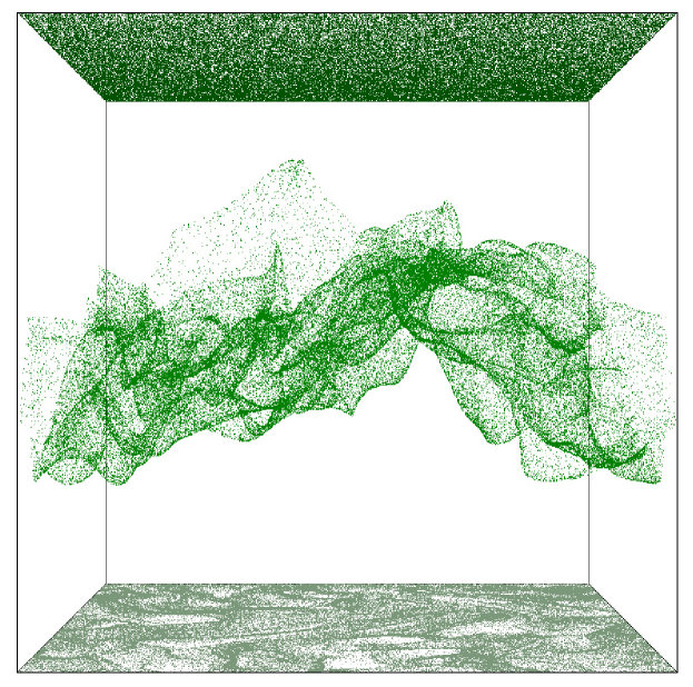
Figure 1: Particle distribution in the initial homogeneous configuration at $z=L$ (upper plane), at an intermediate time (crumpled surface) and particles finally deposited at the lower plane $z=0$.

After the flow has reached statistical steady state, $N=1.2\times 10^{6}$ particles are initialized with homogeneously random positions on a plane at fixed horizontal position $z_{0}=L$. The trajectory of each of them is evolved with Eq. (3). The associated Jacobian matrix $\mathbb{J}_{\alpha\beta}(t)$ giving deformations close to that trajectory is simultaneously evolved with Eq. (6) and initial condition $\mathbb{J}_{\alpha\beta}(0)=\delta_{\alpha\beta}$. Fluid velocity and its gradients are calculated by third-order spatial interpolation on the particles’ positions. The integration time step $dt$ is chosen to be smaller than the time needed to cross a grid cell, which is equal to satisfying the condition $v_{s}dt/dx<1$, where $dx=L/M$. Deformation of the evolving surface is characterized by its tangent vectors ${\bf t}_{1}(t)$ and ${\bf t}_{2}(t)$, given by the first two columns of $\mathbb{J}_{\alpha\beta}(t)$, and by the normal vector ${\bf n}(t)={\bf t}_{1}(t)\times{\bf t}_{2}(t)$. To limit numerical errors arising from exponentially different values of the components of $\mathbb{J}_{\alpha\beta}(t)$ a Gram-Schmidt orthonormalization is applied periodically to the vectors ${\bf t}_{1}(t)$, ${\bf t}_{2}(t)$ and ${\bf n}(t)$ and a new initial condition for $\mathbb{J}_{\alpha\beta}$ is built by using the resulting vectors as columns. The stretching factor $S$ in Eq. (7) is computed as a product of the partial stretching factors obtained before each reinitialization. We consider $17$ different values of the settling velocity $v_{s}$. The largest values do not satisfy the constraint imposed by $St<1$ (a validity condition for the model, see section II), but $St=1$ is clearly marked in every figure.

As we let particles fall and be transported by the flow, we observe the deformation of the initially flat and homogeneous distribution of particles into a crumpled surface, see Fig. 1. Since ${\bf\nabla}\cdot{\bf u}=0$ the dynamics defined by Eq. (3) is also incompressible (${\bf\nabla}\cdot{\bf v}=0$), and we expect that a homogeneous distribution (in the three-dimensional space) is recovered after a sufficient number of eddy turnover times. Such a return to homogeneity can be obtained either at large times or, equivalently, at large depths. At finite times or depths, we suggest that the settling parameter $\Phi=v_{s}/U$ determines the morphology of the surface.

Integration of particle trajectories is performed until the particles reach the bottom plane at $z=0$. In principle, there may be particles that are trapped forever in the flow above the bottom plane, but for the parameters used here all particles arrive at the bottom plane within a finite time. When a particle reaches the bottom plane at $z=0$, we register its position ${\bf X}(t_{h})=({\bf x}_{h},0)$, its velocity ${\bf v}$ and its arrival time $t_{h}$. With this information and the values of the stretching computed along the trajectory we are able to compute the total stretching $S$, the projection $P$ and the total factor $F$ for each particle.

We recall that the simulations of the fluid dynamics are implemented with periodic boundaries, which means that the accumulation plane is neither a physical barrier nor a wall. For the particles, however, the domain is periodic only in the horizontal directions. In the vertical direction, it is semi-finite with an absorbing boundary condition at the bottom, on the accumulation plane, where particle trajectory integration is stopped. We also remark that caution should be taken when considering fast settling particles in a periodic flow woittiez2009 ; ireland2016 , since they can perceive spurious correlations of the turbulent flow, when the time it takes a particle to fall through the domain is smaller than the correlation time of the underlying flow. In standard setups such as ireland2016 , particles were recirculating along the periodic domain and then, if falling sufficiently fast, they could artificially encounter the same eddy several times. In our setup a fast particle can sample parts of the same eddy twice at most. Also, the density factor accumulates stretching contributions from the whole particle trajectory, of which the boundary region is just a tiny part. Thus, we expect the results described below to be independent of the use of periodic boundary conditions. In fact we have computed the average time-dependent stretching on particles with trajectories stopped at the same accumulation layer, but with a domain size $L$ for the flow simulation twice as large, and found no difference with the result under the setup described here.

IV Results and discussion

IV.1 Direct inspection of spatial variations

Particles reach the bottom with different times of arrival. Hence, neighboring particles on the accumulation plane may have visited different regions of the domain, experienced very different histories of stretching and folding and finally be collected at different moments. Similarly, particles that are initially close may have diverged and concluded their trajectories in very distant regions and at very diverse times as well.

First we aim to obtain a direct quantitative insight to the inhomogeneities in the distribution of particles collected on the accumulation plane. A suitable way to characterize this concentration field is to compute a coarse-grained surface density $\rho_{ij}$, where the indices $(i,j)$ label a set of boxes on the collecting plane: particle positions on that collecting plane are located within a two-dimensional grid with resolution $M_{B}$ and counted in each cell of size $L_{B}=L/M_{B}$. So that, $\rho_{ij}=n_{ij}/L_{B}^{2}$, where $n_{ij}$ is the number of particles in the cell $(i,j)$. Summing over all cells one obtains the total number of particles as $\sum_{i,j=1}^{M_{B}}n_{ij}=N$. The initial density, namely $\rho_{0}$, is equal to $N/L^{2}$, so that $\rho_{ij}/\rho_{0}=(n_{ij}L^{2})/(NL_{B}^{2})=(n_{ij}M_{B}^{2})/N$. In the homogeneous case when $n_{ij}=N(L_{B}/L)^{2}$, we obtain $\rho_{ij}/\rho_{0}=1$. If the particle distribution becomes inhomogeneous, the presence of voids and clusters will be registered where $\rho_{ij}/\rho_{0}<1$ and $\rho_{ij}/\rho_{0}>1$, respectively.

In the absence of folds, $\rho_{ij}/\rho_{0}$ is a coarse-grained version of $F({\bf x}_{h})=\rho({\bf x}_{h})/\rho_{0}$. If more than one branch of the surface appears at a particular position due to some folding of the surface, $\rho/\rho_{0}$ will correspond to a sum of the coarse-grained values of $F$ characterizing the different branches.

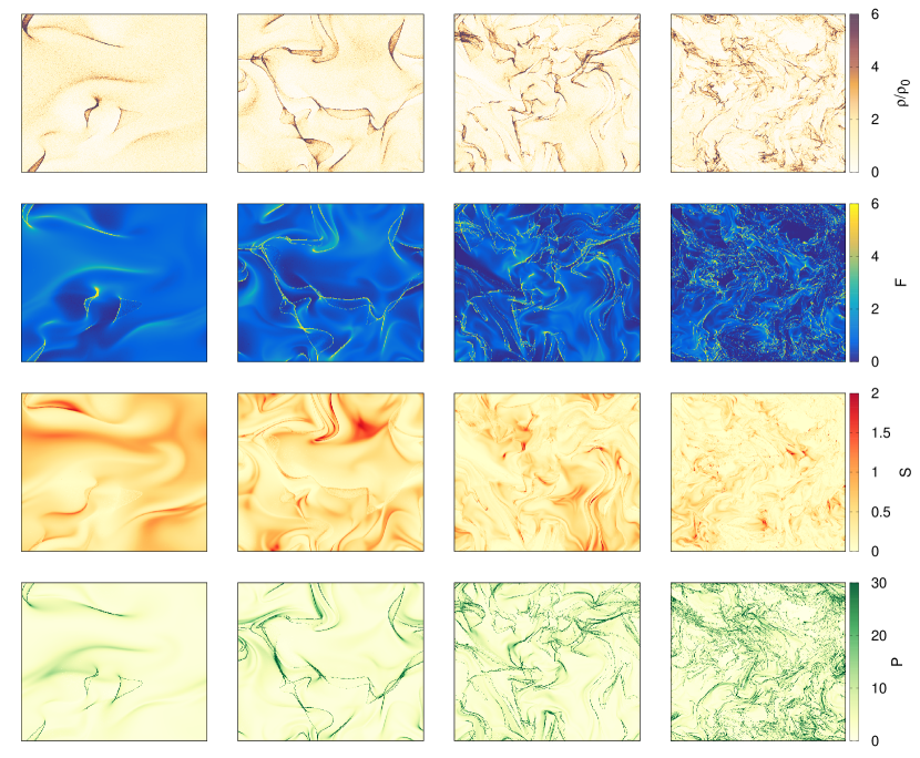
Figure 2: Color map of the final distribution at the accumulation plane of the coarse-grained particle density $\rho/\rho_{0}$ (first row, box resolution of the coarse-graining is $M_{B}=512$), the total density factor $F({\bf x}_{h})$ (second row) and the separated contributions due to the stretching $S({\bf x}_{h})$ and the projection $P({\bf x}_{h})$ factors (third and fourth row). $Re_{\lambda}=19,30,60,93$ in the four columns from left to right. Computations are for $\Phi=3$, a value for which a large Poisson dispersion index $\chi$ is attained.

In Figure 2, examples for the spatial distribution of the coarse-grained particle density, the total density factor, and the separated contributions of stretching and projection are shown on the accumulation plane for a given settling parameter (chosen near the maximal observed inhomogeneity, as characterized by the Poisson dispersion index $\chi$ defined below). $F$, $S$ and $P$ have also been coarse-grained by taking the arithmetic average in the same cells as those that define $\rho_{ij}$. (Note that summation over different branches is not actually performed for this qualitative inspection.) We observe the emergence of clustering of particles in the coarse-grained density and in the total density factor, which are in reasonable agreement with each other, even if a perfect agreement is not expected, since the presence of folds is obvious. At most points we observe that $S<1$ meaning that the infinitesimal area $|{\bf t}_{1}\times{\bf t}_{2}|~{}dA_{0}$ has grown larger than the original $dA_{0}$. Also, the most noticeable features in $P$ are large values that arise from the lines at which ${\bf\hat{n}}\cdot{\bf v}\to 0$, i.e. from the caustic lines at which $P$ diverges. In fact, a comparison with the maps of stretching and projection suggests that the largest inhomogeneities are due to the formation of caustics, the abundance of which increases with the Reynolds number $Re_{\lambda}$, leading to the formation of a complex web of filaments. The dominance of caustics is similar to the case of advection of inertial heavy particles, but in that case they arise from the compressibility of the particle flow wilkinson2005 ; gustavsson2014 , whereas here the particle flow is incompressible ($\nabla\cdot{\bf v}=0$) and develops caustics because of the two-dimensional character of the initial distribution, together with the bending action of the flow and the projection effect on the bottom surface. These three effects concur in the formation of the final distribution of particles.

IV.2 Statistical characterization of inhomogeneities in the collecting plane

Next, we quantitatively investigate the degree of inhomogeneity and its dependence on $\Phi$ and $Re_{\lambda}$ by evaluating the so-called Poisson dispersion index $\chi$ of the particle number distribution $n_{ij}$ defined over the coarse-graining boxes of the accumulation plane. We also discuss implications of the choice of the box size $L_{B}$ for coarse-graining.

As a first step, the average and the standard deviation of the set of values $\{n_{ij}\}$ on the accumulation plane are considered (similarly as in drotos2019 ; monroy2019 ). Since the number of particles is conserved and periodic boundary conditions are prescribed in the horizontal direction, the spatial average of $n_{ij}$ is the same as the initial number: $\overline{n_{ij}}=n_{0}=N/M_{B}^{2}$ (where the bar represents the average with respect to boxes). Simple quantifiers of inhomogeneity are the standard deviation $\sigma_{n}$ and its square, the variance. The latter is conveniently normalized by $n_{0}$ to quantify deviations from a homogeneous Poisson distribution by the Poisson dispersion index as $\chi=\sigma_{n}^{2}/\overline{n}=\sigma_{n}^{2}/n_{0}$. Note that $\chi=1$ corresponds to a homogeneous but random distribution, describing particles arriving at uniformly random positions on the accumulation plane. In such a case, a nonzero standard deviation $\sigma_{n}$ results from the finite number of particles, which, after coarse-graining, leads to a Poisson distribution of $n$ over the boxes. True inhomogeneity, with clusters and voids, is indicated by $\chi\neq 1$.

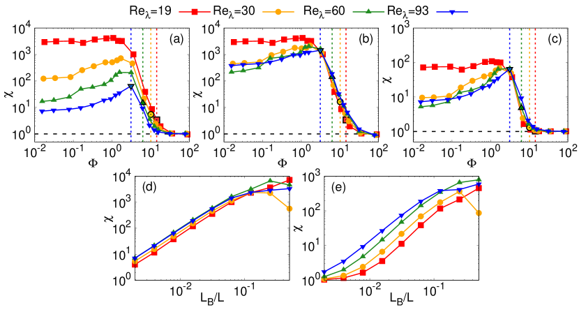
Figure 3: The Poisson dispersion index $\chi$ computed for the two-dimensional horizontal distribution of particles at the accumulation level as a function of the settling parameter $\Phi$ (a-c) and the coarse-graining box size $L_{B}$ (d-e) for different values of $Re_{\lambda}$. $L_{B}=2L/M$ (a), $L_{B}=L/16$ (b) and $L_{B}=L/128$ (c), $\Phi=3.35$ (d), $\Phi=6.7$ (e). The settling parameter $\Phi$ corresponding to $St=1$, an upper bound of the validity range of 3, is marked by a black contoured symbol and a dashed line for each $Re_{\lambda}$.

How to choose $L_{B}$ for coarse-graining is not obvious. On the one hand, it is not meaningful to take $L_{B}$ below some mean distance between the particles ($\rho^{-1/2}$). On the other hand, $L_{B}$ may be chosen below the spatial resolution $L/M$ of the fluid flow in order to resolve small-scale folds of the particle sheet, which may have an important effect on the observed inhomogeneity. In Fig. 3a) we present the dispersion index as a function of the settling parameter $\Phi$, and where the size of the coarse-graining boxes is chosen to depend on the resolution $M$ of the fluid model as $L_{B}=2L/M$ and thus also on the Reynolds number, cf. Table 1. This box size is near the smallest characteristic scale (the Kolmogorov length scale) of the fluid motion, but varies between relatively coarse ($L/16$) and much finer ($L/128$) values compared to the domain size. Irrespective of $Re_{\lambda}$, particles are found uniformly distributed on the accumulation plane for large $\Phi$ ($\chi\approx 1$), which is a result of the lack of time for the surface to deform (remember that the surface is represented by randomly initialized particles). At intermediate $\Phi$ we start to observe considerable inhomogeneities characterized by $\chi>1$. A maximum of clustering is found between $\Phi=1$ and $4$, when the particle settling velocity $v_{s}$ is of the same order as the root-mean-square fluid velocity $U$. Note also that the accumulation plane would be reached during one unit of the integral time scale $T$ by a particle uniformly settling with $\Phi$ between $1.5$ and $2.5$ in all simulations, see Table 1. Decreasing $\Phi$ further results in a slight decrease of $\chi$.

Fig. 3a also shows that the limiting value of $\chi$ for $\Phi\to 0$ strongly depends on the Reynolds number. For any $\Phi$, in fact, a higher $Re_{\lambda}$ implies a smaller $\chi$. This result means that inhomogeneities at the Kolmogorov length scale are actually attenuated as the velocity field becomes increasingly complicated, which can be attributed to an increased mixing.

One may, of course, also compare inhomogeneities observed at the same spatial resolution $L_{B}$ in flows with different Kolmogorov scale and $Re_{\lambda}$. Results are shown for a large and a small $L_{B}$ in Figs. 3b and 3c, respectively. While the characteristics of the individual lines are the same as in Fig. 3a), curves for different $Re_{\lambda}$ cross at a value of $\Phi$ a bit above $\Phi=1$. That is, it depends on the settling velocity whether increasing turbulence strength attenuates or enhances inhomogeneity observed at a given spatial resolution. The settling parameter of Fig. 2 is just large enough to fall into the latter category.

It is worth noting that inhomogeneities observed at a small resolution $L_{B}$ are typically weaker than those at a larger resolution for any given Reynolds number: compare the range of $\chi$ between Figs. 3b and 3c, and see Figs. 3d and 3e for a direct representation for given (large) values of $\Phi$. On the finest spatial scales, where for fast settling initial randomness dominates over later mixing, $\chi$ appears to converge to $1$.

We now see that the degree of observed inhomogeneity strongly depends on the spatial resolution, but its dependence on the settling velocity and on the turbulence strength ($Re_{\lambda}$) is robust for any given resolution. We can conclude about the existence of two regimes from the point of view of parameter dependence, one for large $\Phi$ and one for small $\Phi$, where the effect of increasing mixing by the flow is opposite. We will elaborate on this point and on the crossover between the two regimes in the next subsection, where we analyze the mechanisms underlying our observations.

When using the correlation dimension falkovich2002 ; bec2003 ; sozza2018 for estimating inhomogeneities as a function of $\Phi$ (not shown), the same qualitative behavior is observed as with the Poisson dispersion index. This suggests that our conclusions are robust, and they do not depend on the choice of the particular statistical quantifier.

IV.3 Statistics of stretching and projection over trajectories

We attempt to explore the mechanisms leading to the dependence of $\chi$ on $\Phi$ and $Re_{\lambda}$ presented in Fig. 3 by investigating corresponding properties of the two mechanisms contributing to inhomogeneities, namely the stretching and the projection effects. For the statistical quantification of their local characteristics, we treat different branches of the sedimenting surface separately, without any summation. Furthermore, at difference with Sect. IV.2 and drotos2019 ; monroy2019 , we explore in this section the statistics with respect to the uniform distribution of particles in the initial layer, or equivalently, we weight each particle trajectory equally. This provides a point of view complementary to the statistics over boxes in the collecting layer explored in Sect. IV.2 to compute $\sigma_{n}$ and $\chi$. In particular, we compute here arithmetic averages $\langle A\rangle$, standard deviations $\sigma_{A}$ and correlation coefficients of $A=S$, $P$ and also $F$ over the individual values obtained for the individual particles, e.g.:

$$\langle A\rangle=\dfrac{1}{N}\sum_{k=1}^{N}A_{k}.$$ (8)

where $k$ runs over different particles. In the limit of infinitely many particles,

$$\langle A\rangle =\frac{\int A({\bf x}_{0})\,\mathrm{d}^{2}{\bf x}_{0}}{\int 1\,\mathrm{d}^{2}{\bf x}_{0}}$$

$$=\frac{\int A({\bf x}_{h})F({\bf x}_{h})\,\mathrm{d}^{2}{\bf x}_{h}}{\int F({\bf x}_{h})\,\mathrm{d}^{2}{\bf x}_{h}},$$ (9)

where the $d{\bf x}_{0}$ integrals are taken over the complete initial release plane, and the integral over $d{\bf x}_{h}$ over each branch of the surface sedimented on the collecting plane with a subsequent summation of the values obtained for the different branches. We have used that the number of particles is conserved, $\rho_{0}\mathrm{d}^{2}{\bf x}_{0}=\rho({\bf x}_{h})\mathrm{d}^{2}{\bf x}_{h}$. The second expression in (9) illustrates why such a uniform weighting according to the initial (uniform) distribution of the particles is equivalent to weighting the points in the collecting plane with the total density factor $F$ (or the final density at those points if the sedimenting surface reaches the collecting plane in a single branch). Note that this kind of evaluation for a finite number $N$ of particles corresponds to an ”implicit” coarse-graining on the collecting plane, with a grid provided by the particles’ positions.

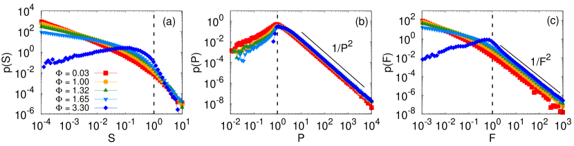
Figure 4: Probability density functions (statistics over released particles) of stretching $p(S)$ (a), of projection $p(P)$ (b) and of the total density factor $p(F)$ (c), at $Re_{\lambda}=60$ for the indicated values of the settling parameter $\Phi$.

To better understand the contribution of stretching and projection to the inhomogeneities, we first report in Figure 4 the probability density functions of $S$, $P$, and $F$ over the individual trajectories. The distribution of $F$ combines the behavior of $S$ and $P$. The low values of the total density factor $F\ll 1$ are controlled by low values of stretching, whereas large values $F\gg 1$ are produced by the large values in $P$, associated with caustics. The distributions of stretching appear to behave as power laws for small values of the settling parameter $\Phi$. When $\Phi$ is below roughly $1$ (the value giving the maximum of clustering, see Figs. 3a-c), the weight given to very small values of $S$ increases as $\Phi$ decreases, since the areas of the surface elements arriving on the collecting plane can grow without limits. On the contrary, the distribution of $P$ remains mostly unchanged for varying values of $\Phi$ and does not depend on $Re_{\lambda}$ (not shown), revealing a universal geometric feature of the projection near caustics. Indeed in Figure 4 we observe $p(P)\sim P^{-2}$ and $p(F)\sim F^{-2}$ for $P\gg 1$ and $F\gg 1$, respectively, which can be explained by the formation of caustics. It is a well-known result that, generically, the density profile at a line caustic diverges as $F\propto x^{-1/2}$, where $x$ is the transverse spatial distance to the caustic wilkinson2005 . Considering the transformation between variables $x$ and $F$ (assuming homogeneity in the direction parallel to the caustic), $p(F)dF=p(x)dx$, and that, as seen before, the density factor gives the proper weight to the horizontal locations $p(x)\sim F$ one obtains $p(F)=|dx/dF|p(x)\propto F^{-2}$.

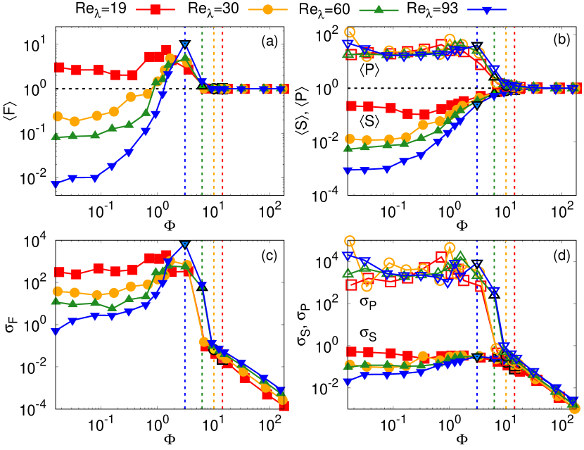
Figure 5: Average and standard deviation of $F$, $S$ and $P$ for different values of $Re_{\lambda}$ as a function of the settling parameter $\Phi$. (a) Average of $F$, (b) average of $S$ and $P$, (c) standard deviation of $F$, (d) standard deviation of $S$ and $P$. The settling parameter $\Phi$ corresponding to $St=1$, an upper bound of the validity range of 3, is marked by a black contoured symbol and a dashed line for each $Re_{\lambda}$.

To place the corresponding properties of $S$ and $P$ into a narrower context, we now investigate the average and standard deviation (statistics over released particles) of the total density factor $F$. $\langle F\rangle$ and $\sigma_{F}$ are plotted in Fig. 5. The former characterizes the average dilution ($\langle F\rangle<1$) or concentration ($\langle F\rangle>1$) of particles on the collecting plane with respect to the initial release density $\rho_{0}$ (remember that different branches generated by folding of the falling surface are treated separately). Meanwhile, $\sigma_{F}$ describes the degree of inhomogeneity among the different particles.

The shape of $\sigma_{F}$ as a function of $\Phi$ in Fig. 5 is very similar to that of $\chi$ in Fig. 3 (except for the large-$\Phi$ asymptotics, of course), which suggests that the accumulated inhomogeneities (represented by $\chi$) are closely related to the trajectory-wise processes of stretching and projection, as opposed to summation of the density over different branches of the sedimented surface, which could also have a dominating effect. Note, however, that a quantitative comparison would be difficult, so that summation may well be important, too.

For increasing $\Phi$, $\langle F\rangle$ converges to $1$, as expected in the lack of time for deformation and bending, while it generally exhibits a shift toward net dilution, or area expansion, for decreasing $\Phi$ below $\Phi\approx 1$, which will be understood by analyzing $S$ and $P$. Between $\Phi=1$ and $10$, $\langle F\rangle$ exhibits a prominent maximum, just like $\chi$ and $\sigma_{F}$. This maximum suggests again that either $v_{s}\approx U$ or a settling time near the integral time scale (or both circumstances) result in a kind of resonance where maximal net deformation and maximal inhomogeneity in the deformation takes place. This resonance represents, furthermore, a crossover between the regimes of large and small $\Phi$ with different tendencies.

Very close to $\Phi=1$, just as for $\chi$, we find a crossing in the $Re_{\lambda}$-dependences, too: for $\Phi<1$, an increasing Reynolds number results in a shift toward net dilution or expansion (decreasing $\langle F\rangle$) and a decrease in inhomogeneity ($\sigma_{F}$), but these tendencies revert near $\Phi=1$. We conclude that the effects of increasing the strength of turbulence are far from trivial but are certainly different in the regimes of small and large settling parameter.

Much insight becomes accessible about explanations for the above tendencies by analyzing the statistics of $S$ and $P$. The decay of both $\sigma_{S}$ and $\sigma_{P}$ in Fig. 5 follows the same power law for large $\Phi$ as $\sigma_{F}$. $\sigma_{S}$ is not affected much by the resonance between $\Phi=1$ and $10$, but typically becomes slightly decreasing for $\Phi<1$, while exhibiting only a minor degree of inhomogeneity there. Based on this observation and the similar magnitudes of $\sigma_{F}$ and $\sigma_{P}$ in Figs. 5, most of the inhomogeneity in $F$ near and below the resonance might appear to originate from the inhomogeneity of $P$. Note, however, the rather erratic behavior, lacking a clear tendency, of $\sigma_{P}$ for decreasing $\Phi$, contrasting the behavior of $\sigma_{F}$. While this relationship will be further commented on later, and a comprehensive understanding of all aspects is beyond the scope of the current analysis, a universal conclusion about the small-$\Phi$ behavior of the degree of inhomogeneity in any quantity seems to be a convergence to some constant value, in spite of the arbitrarily long time available for deformation for $\Phi\to 0$.

This behavior of the standard deviation appears to apply to mean values as well, as Fig. 5 illustrates for $\langle S\rangle$ and $\langle P\rangle$. With $\langle P\rangle$ being mostly constant for $\Phi<1$, the decrease in $\langle F\rangle$ can naturally be linked to the decrease of $\langle S\rangle$ for decreasing $\Phi$ observed in this regime in Fig. 5. The decrease in $\langle S\rangle$ below $1$ actually describes a stretching (expansion, corresponding to a dilution of the density) of increasing strength, which is presumably related to the longer time available for the development of deformation. The same effect may underlie the even sharper response of $\langle P\rangle$ for decreasing $\Phi$ between $10$ and $1$, before the increase of $\langle P\rangle$ saturates. The difference in the sharpness and the saturation of $\langle P\rangle$ is what gives rise to the resonance-like behavior in $\langle F\rangle$, even though $F=SP$ only pointwise, and $\langle F\rangle\neq\langle S\rangle\langle P\rangle$ in general due to spatial correlations.

Fig. 5 also provides with the opportunity to study the effects of varying the Reynolds number. Both $\langle P\rangle$ and $\sigma_{P}$ depend weakly and irregularly on $Re_{\lambda}$ for $\Phi<1$. This might be regarded as an indication of a saturation in all effects of projection, which cannot be enhanced further by modifying the circumstances (Reynolds number and settling parameter). The explanation of such a saturation might be the reaching of a ”maximal randomness” in the orientation of the normal vector of an arbitrarily chosen point of the sedimenting surfacedrotos2019 .

The fact that $\langle S\rangle$ does not saturate but decreases with increasing $Re_{\lambda}$ in the same range of $\Phi$ (Fig. 5, similarly to $\langle F\rangle$) suggests that a similar saturation is not reached in the stretching, the net effect of which may grow without any limit, as shown by the distribution of $S$ in Fig 4a. The dependence of $\langle S\rangle$ (and $\langle F\rangle$) on $Re_{\lambda}$ might simply be understood as stronger deformation resulting from stronger turbulence. Especially in view of this, explaining why inhomogeneity is attenuated with increasing $Re_{\lambda}$ as indicated by $\sigma_{S}$ might be linked to the long-term homogenization in an increasingly complicated flow with increasing mixing capability. The attenuation of inhomogeneity with decreasing $\Phi$ might be explained in a similar way but relying on the longer time available for mixing instead of the increasing mixing capability of the flow. How $\sigma_{S}$ depends on $Re_{\lambda}$ and $\Phi$ for $\Phi<1$ appears to be transferred to $\sigma_{F}$ (Fig. 5), which suggests that inhomogeneities in stretching do have an important effect on the final inhomogeneities in spite of their much smaller magnitude.

By now, mixing is understood to be a central process in shaping the inhomogeneities for $\Phi<1$. We have seen that more mixing (smaller $\Phi$ or larger $Re_{\lambda}$) attenuates inhomogeneities on the long term (at least when investigated at a predefined spatial resolution, which is determined here by the finite number of particles, cf. Section IV.2). Without mixing, however, there would be no inhomogeneities at all.

We resolve this apparent contradiction by considering the short-term effects of mixing. In particular, when compared to the small-$\Phi$ regime, mixing works in the opposite way in the large-$\Phi$ regime. That is, $\sigma_{P}$ and $\sigma_{S}$ (and also $\langle P\rangle$ and $\langle S\rangle$) increase with increasing $Re_{\lambda}$ (see in Fig. 5). The presumable explanation precisely lies in the time available for mixing, which is around or less than the integral time scale. It seems plausible that saturation is not reached in the effects of the projection, nor homogenization is performed, which is confirmed by $\sigma_{P}$ and $\sigma_{S}$ growing from $0$ with decreasing $\Phi$ and increasing $Re_{\lambda}$ in Fig. 5. As long as the sheet is not deformed very much, stronger turbulence or longer time naturally results in the intensification of both the net effects of deformation and their inhomogeneity. For the net effects $\langle P\rangle$ and $\langle S\rangle$, this is similar to the $\Phi<1$ regime except that $\langle P\rangle$ saturates there.

Comparing the $Re_{\lambda}$-dependence of $\langle S\rangle$ and $\langle P\rangle$ for $\Phi\gtrsim 1$, the former becomes weaker than the latter, and this is what we suppose to yield a change in the dependence of $\langle F\rangle$ on $Re_{\lambda}$ between the two regimes. At the same time, the similar change for $\sigma_{F}$ is more straightforwardly explained by the same change for $\sigma_{S}$ and $\sigma_{P}$, corresponding to an inherent difference between the short-term and long-term behaviors. It is interesting to observe that introducing stronger turbulence enhances and attenuates inhomogeneities before and after the crossover.

So far, we have learnt that observable inhomogeneities (as in Fig. 3) are strongly determined by trajectory-wise processes (investigated in Fig. 4 and 5). Increasing mixing by the flow has been identified to introduce and enhance inhomogeneities on the short term, and to attenuate them on the long term (at the spatial resolution corresponding to the finite number of particles). We point out, however, that summation over the increasingly numerous branches of the falling layer may contribute to the attenuation of inhomogeneities. Irrespective of that, the strongest inhomogeneities have been linked to the projection of the falling layer onto the accumulation plane (e.g. caustics). However, the impacts of projection have been found to saturate after entering the well-mixed regime, where the parameter dependence of stretching effects appears to be dominant, conforming with the above-mentioned attenuation of observable inhomogeneities.

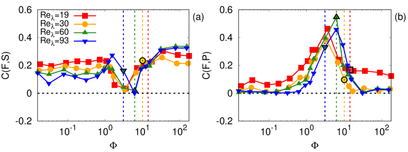
Figure 6: Pearson correlation coefficients: (a) $C(F,S)$ and (b) $C(F,P)$ for different values of $Re_{\lambda}$ as a function of the settling parameter $\Phi$. The settling parameter $\Phi$ corresponding to $St=1$, an upper bound of the validity range of 3, is marked by a black contoured symbol and a dashed line for each $Re_{\lambda}$.

The latter claims, indirectly derived from Fig. 5, are supported by an analysis of spatial correlations. We compute the Pearson correlation coefficient of $F$ with $S$ and $P$ ($C(F,S)$ and $C(F,P)$) using statistics over particles. The value of the correlation coefficient is influenced by both net effects and inhomogeneities. If stretching and projection were uncorrelated (which is not the case, see Fig. 2), we would have $C(F,S)=\frac{\sigma_{S}}{\sigma_{F}}\langle P\rangle$ and a corresponding formula for $C(F,P)$, which suggests that both averages and standard deviations are relevant monroy2019 .

Results for the correlation coefficients are plotted in Fig. 6. For increasing $\Phi$ beyond the crossover, stretching seems to be dominant in forming the spatial structures of the final density (although this is not observed for all Reynolds numbers). This suggests that undulations of the surface become negligible compared to the effect of stretching for increasing $\Phi$, in accordance with the same conclusion of monroy2019 . In the vicinity of the resonance, projection takes over, and the correlation with stretching falls to zero. This is presumably due to the increase in the inhomogeneity of projection, without a similar increase for stretching (see Fig. 5d). Such a result is in agreement with the qualitative observation of the spatial distributions in the proximity of the resonance, displayed in Fig. 2, where the filamentary structures of $P$ and $F$ appear to be well correlated. The dominance reverts again for $\Phi<1$, which is in accordance with the observation that both $\langle F\rangle$ and $\sigma_{F}$ follow the corresponding features of $S$ (both as a function of $\Phi$ and $Re_{\lambda}$). In relation with Fig. 5, we explained this via the saturation of $P$, corresponding to the unit vector $\hat{{\bf n}}$ normal to the (wrapped and contorted) surface taking already a random orientation, which cannot become more disordered by decreasing $\Phi$.

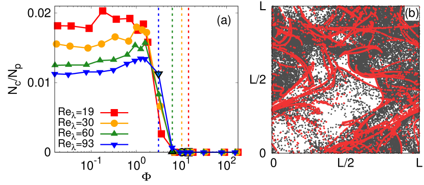
Figure 7: (a) Fraction of particles $N_{c}/N_{p}$ in caustics characterized by having ${\bf\hat{n}}\cdot{\bf v}=0$ (numerically, the requirement is $|{\bf\hat{n}}\cdot{\bf v}|<0.01$). The settling parameter $\Phi$ corresponding to $St=1$, an upper bound of the validity range of 3, is marked by a black contoured symbol and a dashed line for each $Re_{\lambda}$. (b) Positions of the particles sedimented on the collecting plane. In red, particles in caustics as defined above. $\Phi=1$ and $Re_{\lambda}=19$.

In Fig. 7, we present further evidence supporting that the reason for the huge increment in $P$ in vicinity of the resonance (coming from large $\Phi$ where the surface is flat, see Fig. 5), is that caustics appear where the density formally diverges. Thus in Fig. 7a we plot the fraction of particles in caustics (numerically requiring $|{\bf\hat{n}}\cdot{\bf v}|<0.01$) as a function of $\Phi$, observing the two regimes: very small for large values of $\Phi$, and non-negligible values for $\Phi<1$ and any values of $Re_{\lambda}$. The example of Fig. 7b illustrates by a direct plotting of the positions of the particles on the accumulation plane that caustics are closely related to inhomogeneities in the sedimented particles’ distribution. The filamentary pattern of caustic lines in Fig. 7b is recognized to be the same as that of the maxima of $P$ in Fig. 2 and spreads through the collecting plane.

V Conclusions

We performed direct numerical simulations of sinking non-inertial particles in a turbulent flow, exploring a range of settling velocities and Reynolds numbers. We focused our attention on the inhomogeneities of the particle distribution that take place when particles released on a plane at a fixed height are collected on a certain accumulation depth.

Although the Lagrangian dynamics is incompressible, advection of the two-dimensional surface by the flow and accumulation on a plane can lead to the emergence of inhomogeneities by a combination of stretching and projection effects drotos2019 ; monroy2019 . Our results indicate the existence of two different regimes from this point of view: the inhomogeneities grow during the initial stages of the dispersion, while they undergo attenuation when approaching the long-term asymptotics of a well-mixed state. With a fixed domain size, the settling time and thus the degree of inhomogeneity in the accumulated density is controlled by the settling velocity: the initial and the long-term regimes are realized for large and small settling velocity, respectively.

Between the two regimes, we have found a ”resonant” range of settling velocity where inhomogeneity can become maximal. The maximum might approximately be determined by the coincidence of the settling velocity with the root-mean-square velocity of the flow, by the coincidence of the typical settling time with the integral time scale of the flow, or by an interplay of the two circumstances.

The range of settling velocity hosting this resonance-like behavior not only marks a change of behavior of the degree of inhomogeneity as a function of the settling velocity itself, but also as a function of the Reynolds number. During the initial transients, a more complicated flow (higher Reynolds number) enhances inhomogeneity, while it facilitates approaching homogeneous mixing in the regime leading to the long-term asymptotics.

We have also investigated the contributions of the two basic inhomogeneizing mechanisms in the two regimes. For large settling velocities, when the surface is bended very little without developing overhangs, stretching is predominant. When getting close to resonant-like settling velocities, folds appear, yielding projection caustics in the sedimented density. For this reason, effects of projection become dominant, and this is responsible for the crossover in some properties at the resonance-like region. With further decrease of the settling velocity, the magnitude of the inhomogeneities remains determined by projection, but the increasing effects of projection saturate soon as mixing becomes strong. The parameter dependence of observable inhomogeneities then conforms with the increasing homogeneity of stretching as mixing becomes stronger, although summation over a large number of different branches of the falling particle layer may also be important.

The above results give an opportunity to comment on some previous work. Although our setup shows a few important differences with the problem of sedimentation in mesoscale oceanic flows addressed in monroy2019 common points are prominent enough to locate the mesoscale oceanic setup on the axis of the settling velocity. In particular, although anisotropy in the velocity field of the ocean is pronounced (with large differences between horizontal and vertical velocities), one can safely state that the settling velocity of typical biogenic particlesmonroy2017 is (several times) larger than vertical velocities of flow. As for the typical sedimentation time, it is the same order of magnitude as the characteristic time scale of the mesoscale oceanic flow. These circumstances may mean that the parameters are not far from the resonance-like maximum of inhomogeneity, and fall into the regime of initial transients identified for $\Phi>1$ in the present paper. Considerable inhomogeneities appear in corresponding oceanic simulations and are enhanced for decreasing settling velocity and increasing mesoscale turbulence strength monroy2019 .

Finally, we indicate the relevance of these studies for sinking biogenic particles in an eddy-resolving oceanic velocity field. A careful study has been performed in monroy2019 for a mesoscale oceanic flow, based on the analysis of monroy2017 of sizes and densities of particles for which our modeling approach is valid. These biogenic particles (examples of which are dead plankton bodies, zoo-plankton fecal pellets, or small aggregates and marine snow) have typical sizes $a$ ranging between $10^{-6}-10^{-3}~{}\mbox{m}$, and typical densities between between $\rho_{p}=1050-2700~{}\mbox{kg}\mbox{m}^{-3}$, so that $\beta$ is bounded between $0.5$ and $1.0$. Oceanic turbulence is characterized by $\varepsilon=10^{-4}-10^{-8}~{}\mbox{m}^{2}/\mbox{s}^{3}$, $\nu=10^{-6}~{}\mbox{m}^{2}/\mbox{s}$ Thorpe2007 , for which we obtain a Kolmogorov length scale $\eta=(\nu^{3}/\varepsilon)^{1}/4=0.3-3~{}\mbox{mm}$, Kolmogorov time scale $\tau_{\eta}=(\nu/\varepsilon)^{1/2}=0.1-10~{}\mbox{s}$, Kolmogorov velocity $u_{\eta}=(\nu\varepsilon)^{1/4}=0.3-3~{}\mbox{mm}/\mbox{s}$ and acceleration $a_{\eta}=(\varepsilon^{3}/\nu)^{1/4}=30-0.03~{}\mbox{mm}/\mbox{s}^{2}$, leading to a Froude number $Fr=\times 10^{-6}-\times 10^{-3}$ and a Stokes number $St=10^{-7}-0.5$. The range of Reynolds numbers used in our numerical simulations indicate that we are dealing with spatial scales of the flow between $6\ cm$ and $1\ m$. Note that our configuration represents two relevant situations in this context: one is sedimentation on the seafloor, and the other is the collection of particles in sediment traps located at a given depth. For this last situation, the impact of boundary conditions at the bottom is irrelevant. However, for sedimentation on the seafloor, in the case of a no-slip boundary condition, a boundary layer close to the bottom is formed and turbulence is drastically reduced and modified there, which, does not affect the processes in the bulk monroy2019 .

References

- (1) G. Falkovich, A. Fouxon, and M. G. Stepanov, “Acceleration of rain initiation by cloud turbulence,” Nature, vol. 419, no. 6903, pp. 151–154, 2002.
- (2) E. J. P. Woittiez, H. J. J. Jonker, and L. M. Portela, “On the combined effects of turbulence and gravity on droplet collisions in clouds: a numerical study,” J. Atmos. Sci., vol. 66, no. 7, pp. 1926–1943, 2009.
- (3) C. L. De La Rocha and U. Passow, “Factors influencing the sinking of poc and the efficiency of the biological carbon pump,” Deep Sea Res. Pt. II, vol. 54, no. 5-7, pp. 639–658, 2007.
- (4) T. DeVries, F. Primeau, and C. Deutsch, “The sequestration efficiency of the biological pump,” Geophys. Res. Lett., vol. 39, no. 13, 2012.
- (5) A. L. Alldredge and C. Gotschalk, “In situ settling behavior of marine snow,” Limnol. Oceanogr., vol. 33, no. 3, pp. 339–351, 1988.
- (6) M. Borgnino, J. Arrieta, G. Boffetta, F. De Lillo, and I. Tuval, “Turbulence induces clustering and segregation of non-motile, buoyancy-regulating phytoplankton,” J. R. Soc. Interface, vol. 16, no. 159, p. 20190324, 2019.
- (7) L. C. Woodall, A. Sanchez-Vidal, M. Canals, G. L. J. Paterson, R. Coppock, V. Sleight, A. Calafat, A. Rogers, B. Narayanaswamy, and R. Thompson, “The deep sea is a major sink for microplastic debris,” R. Soc. Open Sci., vol. 1, no. 4, p. 140317, 2014.
- (8) L. Khatmullina and I. Isachenko, “Settling velocity of microplastic particles of regular shapes,” Mar. Pollut. Bull., vol. 114, no. 2, pp. 871–880, 2017.
- (9) D. A. Siegel and W. G. Deuser, “Trajectories of sinking particles in the Sargasso Sea: modeling of statistical funnels above deep-ocean sediment traps,” Deep Sea Res. Pt. I, vol. 44, no. 9-10, pp. 1519–1541, 1997.
- (10) K. O. Buesseler, A. N. Antia, M. Chen, S. W. Fowler, W. D. Gardner, O. Gustafsson, K. Harada, A. F. Michaels, M. Rutgers van der Loeff, and M. Sarin, “An assessment of the use of sediment traps for estimating upper ocean particle fluxes,” J. Mar. Res., vol. 65, no. 3, pp. 345–416, 2007.
- (11) D. A. Siegel, E. Fields, and K. O. Buesseler, “A bottom-up view of the biological pump: Modeling source funnels above ocean sediment traps,” Deep Sea Res. Pt I, vol. 55, no. 1, pp. 108–127, 2008.
- (12) E. Balkovsky, G. Falkovich, and A. Fouxon, “Intermittent distribution of inertial particles in turbulent flows,” Phys. Rev. Lett., vol. 86, no. 13, p. 2790, 2001.
- (13) J. Bec, “Fractal clustering of inertial particles in random flows,” Phys. Fluids, vol. 15, no. 11, pp. L81–L84, 2003.
- (14) G. Falkovich and A. Pumir, “Intermittent distribution of heavy particles in a turbulent flow,” Phys. Fluids, vol. 16, no. 7, pp. L47–L50, 2004.
- (15) A. Dejoan and R. Monchaux, “Preferential concentration and settling of heavy particles in homogeneous turbulence,” Phys. Fluids, vol. 25, no. 1, p. 013301, 2013.
- (16) J. Bec, H. Homann, and S. S. Ray, “Gravity-driven enhancement of heavy particle clustering in turbulent flow,” Phys. Rev. Lett., vol. 112, no. 18, p. 184501, 2014.
- (17) F. De Lillo, M. Cencini, M. M. Durham, M. Barry, R. Stocker, E. Climent, and G. Boffetta, “Turbulent fluid acceleration generates clusters of gyrotactic microorganisms,” Phys. Rev. Lett., vol. 112, no. 4, p. 044502, 2014.
- (18) A. Sozza, F. De Lillo, and G. Boffetta, “Inertial floaters in stratified turbulence,” Europhys. Lett., vol. 121, no. 1, p. 14002, 2018.
- (19) M. De Pietro, M. A. T. van Hinsberg, L. Biferale, H. J. H. Clercx, P. Perlekar, and F. Toschi, “Clustering of vertically constrained passive particles in homogeneous isotropic turbulence,” Phys Rev E, vol. 91, no. 5, p. 053002, 2015.
- (20) G. Boffetta, J. Davoudi, B. Eckhardt, and J. Schumacher, “Lagrangian tracers on a surface flow: The role of time correlations,” Phys. Rev. Lett., vol. 93, no. 13, p. 134501, 2004.
- (21) P. Monroy, E. Hernández-García, V. Rossi, and C. López, “Modeling the dynamical sinking of biogenic particles in oceanic flow,” Nonlinear Proc. Geophys., vol. 24, no. 2, pp. 293–305, 2017.
- (22) J. R. Taylor, “Accumulation and subduction of buoyant material at submesoscale fronts,” J. Phys. Oceanogr., vol. 48, no. 6, pp. 1233–1241, 2018.
- (23) G. Drótos, P. Monroy, E. Hernández-García, and C. López, “Inhomogeneities and caustics in the sedimentation of noninertial particles in incompressible flows,” Chaos, vol. 29, no. 1, p. 013115, 2019.
- (24) U. Frisch, Turbulence: The legacy of A.N. Kolmogorov. Cambridge University Press, 1995.
- (25) M. R. Maxey and J. J. Riley, “Equation of motion for a small rigid sphere in a nonuniform flow,” Phys. Fluids, vol. 26, no. 4, pp. 883–889, 1983.
- (26) A. Sozza, F. De Lillo, S. Musacchio, and G. Boffetta, “Large-scale confinement and small-scale clustering of floating particles in stratified turbulence,” Phys. Rev. Fluids, vol. 1, no. 5, p. 052401, 2016.
- (27) V. Mathai, E. Calzavarini, J. Brons, C. Sun, and D. Lohse, “Microbubbles and microparticles are not faithful tracers of turbulent acceleration,” Phys. Rev. Lett., vol. 117, no. 2, p. 024501, 2016.
- (28) S. Balachandar and J. K. Eaton, “Turbulent dispersed multiphase flow,” Annu. Rev. Fluid. Mech., vol. 42, no. 1, pp. 111–133, 2010.
- (29) I. Fouxon, “Distribution of particles and bubbles in turbulence at a small Stokes number,” Phys. Rev. Lett., vol. 108, no. 13, p. 134502, 2012.
- (30) P. Monroy, G. Drótos, E. Hernández-García, and C. López, “Spatial inhomogeneities in the sedimentation of biogenic particles in ocean flows: Analysis in the Benguela region,” J. Geophys. Res., vol. 124, pp. 4744–4762, 2019.
- (31) S. B. Pope, P. K. Yeung, and S. S. Girimaji, “The curvature of material surfaces in isotropic turbulence,” Phys. Fluids A, vol. 1, no. 12, pp. 2010–2018, 1989.
- (32) T. Zheng, J. You, and Y. Yang, “Principal curvatures and area ratio of propagating surfaces in isotropic turbulence,” Phys. Rev. Fluids, vol. 2, no. 10, p. 103201, 2017.
- (33) A. G. Lamorgese, D. A. Caughey, and S. B. Pope, “Direct numerical simulation of homogeneous turbulence with hyperviscosity,” Phys. Fluids, vol. 17, no. 1, p. 015106, 2005.
- (34) C. Rosales and C. Meneveau, “Linear forcing in numerical simulations of isotropic turbulence: Physical space implementations and convergence properties,” Phys. Fluids, vol. 17, no. 9, p. 095106, 2005.
- (35) P. Weiss, D. Oberle, D. W. Meyer, and P. Jenny, “Impact of turbulence forcing schemes on particle clustering,” Phys. Fluids, vol. 31, no. 6, p. 061703, 2019.
- (36) A. Sozza, M. Cencini, F. De Lillo, and G. Boffetta, “Scalar absorption by particles advected in a turbulent flow,” arXiv preprint arXiv:2004.10256, 2020.
- (37) P. J. Ireland, A. D. Bragg, and L. R. Collins, “The effect of Reynolds number on inertial particle dynamics in isotropic turbulence. Part 2. Simulations with gravitational effects,” J. Fluid Mech., vol. 796, pp. 659–711, 2016.
- (38) M. Wilkinson and B. Mehlig, “Caustics in turbulent aerosols,” Europhys. Lett., vol. 71, no. 2, p. 186, 2005.
- (39) K. Gustavsson, S. Vajedi, and B. Mehlig, “Clustering of particles falling in a turbulent flow,” Phys. Rev. Lett., vol. 112, no. 21, p. 214501, 2014.
- (40) S. A. Thorpe, An introduction to ocean turbulence. Cambridge University Press, 2007.