Mean square displacement of a free quantum particle
in a thermal state

Abstract

The mean square displacement $\left\langle\left(x(t)-x(0)\right)^{2}\right\rangle$ of the position $x$ of a free particle of mass $m$ at thermal equilibrium is evaluated quantum mechanically. An analytical expression is obtained which shows an initial quadratic increase of the mean square displacement with time and later on a linear growth, with the slope $\hbar/m$, quite at variance with the result from classical statistical mechanics. Results are discussed in relation to observables from helium scattering or spin-echo experiments, and their possible interpretation in terms of the classical and quantum mechanical expression for the mean square displacement of an essentially free particle.

I Introduction

This paper is about the mean square displacement (MSD) $\delta_{x}^{2}(t)=\left\langle(x(t)-x(0))^{2}\right\rangle_{\theta}$ of a thermalized, but otherwise free moving quantum particle, the position of which at time $t$ is $x(t)$. A thermalized state can be characterized by a set of random numbers $\theta$ and $\left\langle\cdot\right\rangle_{\theta}$ is the average in the sense of the arithmetic mean over these states. The main motivation of the present work is the study of the diffusion of particles within the laws of quantum mechanics. Some of the results presented here should also be relevant in quantum transport theory.

In classical mechanics, a particle at thermal equilibrium with its environment moves with statistically distributed positions and velocities. For a free particle, $x(t)=x(0)+vt$ with $\left\langle x(0)\right\rangle_{\theta}=0$ and $\left\langle v\right\rangle_{\theta}=0$ but $\delta_{x}^{2}(t)=\left\langle\left(v\,t\right)^{2}\right\rangle_{\theta}=\left\langle v^{2}\right\rangle_{\theta}\,t^{2}$, and $\left\langle v^{2}\right\rangle_{\theta}=\mbox{$k_{\rm B}$}T\,/\,m$ for a thermal ensemble. Here $T$ is the temperature and $k_{\rm B}$ is the Boltzmann constant . The MSD increases quadratically with time and such a behavior is termed ballistic motion.

In quantum mechanics, the time dependent expectation value of the particle’s position can be given as the trace $x(t)=\mbox{{$\rm Tr$}}\left(\hat{x}\hat{\rho}(t)\right)$, where $\hat{x}$ is the position operator and $\hat{\rho}(t)$ is the time dependent density operator. At thermal equilibrium, the ensemble averaged density operator is constant, $\left\langle\hat{\rho}(t)\right\rangle_{\theta}=\left\langle\hat{\rho}(0)\right\rangle_{\theta}$, so that $x(t)=x(0)$ and $\delta_{x}^{2}(t)\equiv 0$. This is equivalent, however, to the classical result, if $\left\langle v\right\rangle_{\theta}$ is taken instead of $v$ to calculate $\delta_{x}^{2}(t)$. Rather than evaluating the trace with the ensemble averaged density operator, one should evaluate it with a typical member of the thermal ensemble Tolman (1938), and perform the average afterwards. How does $\delta_{x}^{2}(t)$ then look like? To the best of our knowledge, this question does not seem to have received the appropriate attention so far. It is the subject of the present work.

Diffusion has been understood as the result of stochastic processes involving many body interactions since more than a century Einstein (1905); Smoluchowski (1916); Chandrasekhar (1943); Kubo et al. (1992). Theoretical and experimental developments related to diffusion in condensed phases and at surfaces have been continuously reviewed from the prospective of both classical and quantum mechanics in the past 50 years, and references 7; 8; 9; 10; 11; 12; 13; 14; 15; 16; 17 can only partially cover the vast literature on this matter. If a particle is undergoing diffusion, its MSD increases linearly with time, quite contrary to the ballistic motion of a free particle. This property might not be unique to diffusion, however.

Aside this well established consensus, the delocalized nature of the quantum mechanical state of a single particle inherently reflects the diffusive character of its motion Schrödinger (1931); Nelson (1966). Fürth related this character to the uncertainty principle Fürth (1933). The thermal probability density of a single adsorbate, for instance, is extremely delocalized on the adsorption substrate and the uncertainty to find a particle at a specific position in space increases with the size of the space. Under these circumstances it seems worth to investigate how the temporal evolution of the mean square displacement of a particle’s position looks like, when the particle’s dynamics is described entirely by quantum mechanics, say, from the solution of the Liouville-von-Neumann equation for a thermal state or, equivalently, from the solution of the Schrödinger equation with an initial thermal wave packet.

Because quantum mechanical delocalization is a peculiar property of a single particle, this investigation is conveniently conducted, in a first approach, in the independent particle formalism of a many body system. This will be the approach adopted in the present work. Any possible interaction among the particles or between the particles and their environment that leads to a dissipation of energy will be discarded. Friction, which is related to random many body interactions via the fluctuation-dissipation theorem, is consequently excluded in the independent particle formalism. One may argue that, under these conditions, it is meaningless to study diffusion. While it is conceptually interesting to reopen the question of diffusion without friction Fürth (1933); Wallstrom (1994), this is not the aim of the present work. Rather, the focus will be on properties of the time dependent MSD of an independent, thermalized quantum particle, on their relation to properties of diffusion and, quite critically, on their potential relation to observables. Obviously, the neglect of many body interactions is a strong approximation and the present approach will correspondingly yield approximate results, only.

Scattering experiments yield information on particle diffusion by means of the transformation of the inelastic scattering cross section to the space-time pair correlation function $G(r,t)$ formulated by van Hove van Hove (1954). The space Fourier transformation of the pair correlation function is the intermediate scattering function (ISF). The space-time Fourier transformation of the pair correlation function is the dynamical structure factor (DSF). Diffusion coefficients can be extracted as rate constants from the decay of the ISF, or as widths of the DSF, depending on the form of these decays or widths. Many aspects have been covered in the aforementioned reviews. There are also numerous theoretical approaches to diffusion that address quantum mechanical effects. None seem to have addressed the simple question of the quantum dynamical time evolution of the mean square deviation.

It was pointed out by Vineyard Vineyard (1958) and Schofield Schofield (1960) that, for sufficiently long times, the square of the time dependent width of the Gaussian shaped main peak ($r\sim 0$) of the self-part $\mbox{$G_{\rm s}$}(r,t)$ of the pair correlation function can be interpreted classically as the MSD of scatterers. This works particularly well within the jump diffusion model of Chudley and Elliott in the continuous diffusion limit of small jumps or long times Chudley and Elliot (1961). The quantum mechanical evaluation of the MSD will be discussed in relation to this interpretation and to potentially observed quantities. Of particular interest will be a discussion of results from helium scattering experiments of the Xe/Pt(111) system, which mimics an ideal, two dimensional gas Ellis et al. (1999).

The paper is structured as follows: in section 2 the theoretical framework of this paper is explained, working equations are derived, and some concepts are defined. This section also contains the main result of the work, Eq. (13), as well as the definition of some concepts and of a statistical model to interpret some of the numerical results. In section 3 results are discussed. Section 4 concludes the work with a final discussion of its perspectives.

II Theory

II.1 Quantum mechanical approach to $\delta_{x}^{2}(t)$ in the independent particle formalism

In the present work the system to be considered consists of an individual particle of mass $m$, the states of which can be described by the time dependent density operator $\hat{\rho}(t)$. The latter is obtained as a solution of the Liouville-von-Neumann equation $\hat{\rho}(t)=\hat{U}(t)\hat{\rho}(0)\hat{U}^{\dagger}(t)$, where $\hat{U}(t)=\exp(-\mbox{{$\rm i$}}\hat{H}t/\hbar)$, $\hat{H}$ is the system’s Hamiltonian, $h$ is the Planck constant Note (1) and $\hbar=h/2\pi$. $\hat{\rho}(0)$ is the initial density operator.

A thermal state of a quantum system is appropriately defined in the basis of the system’s eigenstates $\lvert{\phi_{n}}\rangle$ ($n=1,2,\ldots$), whose energies are $E_{n}$. Without loss of generality, we may assume a countable set of states. In the ensemble averaged view of statistical mechanics Tolman (1938) the henceforth generated density operator matrix of a thermal state is diagonal; $\mbox{$\langle{\phi_{n}}\rvert$}\hat{\rho}^{(T)}\mbox{$\lvert{\phi_{n}}\rangle$}\equiv{\rho}^{(T)}_{nn}$ are the time independent thermal populations ${\rho}^{(T)}_{nn}(t)=\exp(-E_{n}/\mbox{$k_{\rm B}$}T)/Q(T)={\rho}^{(T)}_{nn}(0)$, while the off-diagonal elements vanish. Here, $Q(T)$ is the canonical partition function. Indeed, in the ensemble average, the thermal density operator commutes with the system’s Hamiltonian and is therefore constant. In such a view, expectation values of observables in thermal states are themselves constants. If the MSD of a quantum particle is defined with $x(t)$ being the expectation value in the thermal state as given above, this quantity vanishes identically, independently of whether the particle moves freely or not.

In ref. 27 the MSD of a quantum particle was defined in the context of a uniform quantum multibaker map for 1D quantum walks within a random matrix theory. It can be written in terms of a time dependent evolution as $\delta_{x}^{2}(t)={\rm Tr}(\hat{\rho}\;(\hat{x}(t)-\hat{x}(0))^{2})$. In this definition, $\hat{x}(t)$ is the time dependent position operator in the Heisenberg picture and $\hat{\rho}$ is the equilibrium density operator. We note that there is no operator $\hat{O}$ such that $\hat{x}(t)-\hat{x}(0)=\hat{U}^{\dagger}(t)\hat{O}\hat{U}(t)$. Therefore, the same definition cannot be given in the Schrödinger picture. The result of a quantum dynamical calculation must not depend on the specific picture used, therefore the definition extracted from ref. 27 is not further considered here.

In this work we shall view individual members of the quantum thermal ensemble Tolman (1938). Such states can be characterized by a set of random phases $0\leq\theta\leq 2\pi$, as will be explained below. In this view the off diagonal elements of the density operator matrix are the non-vanishing, time dependent coherences ${\rho}^{(T)}_{nm}(t)$ ($n\neq m$). Coherences reflect random fluctuations of the density matrix which do vanish, however, upon statistical average. These fluctuations are essential for the calculation of the MSD in the present work. Randomness is also key in a potential approach to link the quantum mechanical evolution of the MSD with diffusion.

The mean square displacement (MSD) is hence defined by

$$\delta_{x}^{2}(t)=\left\langle\left(x(t)-x(0)\right)^{2}\right\rangle_{\theta}$$ (1)

where $x(t)=\mbox{{$\rm Tr$}}\left(\hat{x}\hat{\rho}^{(T)}(t)\right)$ is the quantum mechanical expectation value of the particle’s position at time $t$ in a typical member state of the thermal ensemble. In Eq. (1) the Schrödinger picture is used, but the same quantity is obtained in the Heisenberg picture, as $\mbox{{$\rm Tr$}}\left(\hat{x}\hat{\rho}^{(T)}(t)\right)={\rm Tr}(\hat{x}(t)\hat{\rho}^{(T)})$.

Consistently with the independent particle formalism, coherences are preserved during the time evolution. The adequateness of this approach to describe the time evolution of a thermal state in general, and diffusion in particular, might nevertheless be questioned. The onset of a thermal equilibrium is the consequence of the interaction between many particles. Strictly, to correctly describe the time evolution of the system’s thermal state, this interaction must be considered and one has to resort to more involved open system quantum dynamical and reduced matrix density treatments Klinger (1983); Kubo et al. (1992); Blum (1996); Vacchini and Hornberger (2009). These techniques will typically lead to quantum master equations which include population evolution and decoherence. Steady state solutions of these equations yield the Boltzmann distribution for the populations of thermal states. Other possibilities are path-integral techniques Calhoun et al. (1996); Miller and Manolopoulos (2005); Fang et al. (2017), quantum Langevin or Bohmian dynamics Nassar and Miret-Artés (2013); Miret-Artés (2018); Mousavi and Miret-Artés (2019).

Instead, in the present approach many body interactions are explicitly excluded. Thermal equilibrium, not its onset, and hence any property of the particle resulting from its contact with the environment is described by the imposed initial condition. The dynamical system is closed, which ensures conservation of level populations and temperature. Any temporal variation of the MSD will hence be obtained within closed system equilibrium thermodynamics, which is a rather uncommon approach to diffusion Kubo et al. (1992). Nevertheless, this approach is totally consistent with that sketched in the introductory section for the ballistic behavior of a free moving classical particle.

II.2 Specific quantum mechanical expressions for $\delta_{x}^{2}(t)$

In this section, and for the purpose of a more general use, the system considered is a particle of mass $m$ moving in a one-dimensional potential, periodic in the lattice constant $a$: $V(x)=V(x+a)$. $\hat{H}$ is the corresponding system Hamiltonian:

$$\hat{H}=-\frac{\hbar^{2}}{2\,m}\,\frac{\displaystyle\partial^{2}}{\displaystyle{\partial x}^{2}}+V(x)$$ (2)

The system is cast in periodic super-cells of length $L=N\times a$. The ratio $a/L=1/N$ can then be considered to be the coverage degree of the one dimensional lattice. Later on, results will be discussed for the specific case of a constant potential, or just $V(x)\equiv 0$.

Let

$$\mbox{$\lvert{\psi(0)}\rangle$}=\mbox{$\lvert{\psi^{(T)}}\rangle$}\equiv\sum\limits_{n}\,\frac{{\rm e}^{\displaystyle-\beta\,E_{n}/2+\mbox{{$\rm i$}}\,\theta_{n}}}{\sqrt{Q}}\,\mbox{$\lvert{\phi_{n}}\rangle$}$$ (3)

be an initial thermal wave packet where the quantities $0\leq\theta_{n}\leq 2\pi$ are random angles, $E_{n}$ and $\lvert{\phi_{n}}\rangle$ ($n=1,2,\ldots$) are eigenvalues and eigenstates of the system’s Hamiltonian $\hat{H}$ defined in Eq. (2), and $Q$ is the canonical partition function:

$$Q=\sum\limits_{n}\,{\rm e}^{\displaystyle-\beta\,E_{n}}$$ (4)

Here and in the following, $\beta\equiv 1/(\mbox{$k_{\rm B}$}T)$. The state defined in Eq. (3) is a typical member of the thermal ensemble Tolman (1938); Quack (1982).

For $t>0$, the thermal wave packet evolves as the solution of the time dependent Schrödinger equation

$$\lvert{\psi^{(T)}(t)}\rangle = \sum\limits_{n}\,\frac{{\rm e}^{\displaystyle-\beta\,E_{n}/2+\mbox{{$\rm i$}}\,\theta_{n}-\mbox{{$\rm i$}}\,E_{n}\,t}}{\sqrt{Q}}\,\mbox{$\lvert{\phi_{n}}\rangle$}$$ (5)

The density operator $\hat{\rho}^{(T)}(t)=\mbox{$\lvert{\psi^{(T)}(t)}\rangle$}\mbox{$\langle{\psi^{(T)}(t)}\rvert$}$ is the solution of the Liouville-von-Neumann equation with initial $\hat{\rho}^{(T)}(0)=\mbox{$\lvert{\psi^{(T)}(0)}\rangle$}\mbox{$\langle{\psi^{(T)}(0)}\rvert$}$. Its matrix elements in the basis of eigenstates are

$${\rho}^{(T)}_{nm}(t)=\mbox{$\langle{\phi_{n}}\rvert$}\hat{\rho}^{(T)}(t)\mbox{$\lvert{\phi_{m}}\rangle$}=\frac{{\rm e}^{\displaystyle-\beta(E_{n}+E_{m})/2}}{Q}\,{\rm e}^{\displaystyle\mbox{{$\rm i$}}\,(\theta_{n}-\theta_{m})-\mbox{{$\rm i$}}\,(E_{n}-E_{m})\,t/\hbar}$$ (6)

Eqs. (5) and (6) are valid in an independent particle formalism and, as assumed throughout this work, in the high temperature limit, where symmetry restrictions due to the indistinguishability of identical particles are not important.

Following the definition in Eq. (1), the quantum mechanical MSD of the particle is then

$$\delta_{x}^{2}(t) = \left\langle\left(\mbox{{$\rm Tr$}}\left(\hat{x}\hat{\rho}^{(T)}(t)\right)-\mbox{{$\rm Tr$}}\left(\hat{x}\hat{\rho}^{(T)}(0)\right)\right)^{2}\right\rangle_{\theta}=\left\langle\left(\sum\limits_{n}\sum\limits_{j}\,({\rho}^{(T)}_{nj}(t)-{\rho}^{(T)}_{nj}(0))\,x_{nj}\right)^{\displaystyle 2}\,\right\rangle_{\displaystyle\theta}$$ (8)

$$= \frac{1}{Q^{2}}\;\sum\limits_{n}\sum\limits_{j}\sum\limits_{n^{\prime}}\sum\limits_{j^{\prime}}\;{\rm e}^{\displaystyle-\beta\,(E_{n}+E_{j}+E_{n^{\prime}}+E_{j^{\prime}})/2}$$

$$\;\;\;\times\;x_{nj}\;x_{n^{\prime}j^{\prime}}$$

$$\;\;\;\times\;\left({\rm e}^{\displaystyle-\mbox{{$\rm i$}}\,(E_{n}-E_{j})\,t\,/\,\hbar}-1\right)\;\left({\rm e}^{\displaystyle-\mbox{{$\rm i$}}\,(E_{n^{\prime}}-E_{j^{\prime}})\,t\,/\,\hbar}-1\right)$$

$$\;\;\;\times\;\left\langle{\rm e}^{\displaystyle\mbox{{$\rm i$}}\,(\theta_{n}-\theta_{j}+\theta_{n^{\prime}}-\theta_{j^{\prime}})}\right\rangle_{\displaystyle\theta}$$

where $x_{nm}=\mbox{$\langle{\phi_{n}}\rvert$}\hat{x}\mbox{$\lvert{\phi_{m}}\rangle$}$.

The averaged quantities $\left\langle{\rm e}^{\displaystyle\mbox{{$\rm i$}}\,(\theta_{n}-\theta_{j}+\theta_{n^{\prime}}-\theta_{j^{\prime}})}\right\rangle_{\theta}$ yield zero, unless $n=j$ and $n^{\prime}=j^{\prime}$, or $n=j^{\prime}$ and $j=n^{\prime}$. But for $n=j$ (and $n^{\prime}=j^{\prime}$) the matrix elements $x_{nn}$ (and $x_{n^{\prime}n^{\prime}}$) vanish, by symmetry, so that only one double sum results in the expansion:

$$\delta_{x}^{2}(t) = \frac{1}{Q^{2}}\;\sum\limits_{n}\sum\limits_{j}{\rm e}^{\displaystyle-\beta\,(E_{n}+E_{j})}\;\lvert x_{nj}\rvert^{2}$$ (9)

$$\;\;\;\times\;\left({\rm e}^{\displaystyle-\mbox{{$\rm i$}}\,(E_{n}-E_{j})t/\hbar}-1\right)\,\left({\rm e}^{\displaystyle\mbox{{$\rm i$}}\,(E_{n}-E_{j})t/\hbar}-1\right)$$

$$= \frac{4}{Q^{2}}\;\sum\limits_{n}\sum\limits_{j}{\rm e}^{\displaystyle-\beta\,(E_{n}+E_{j})}\;\lvert x_{nm}\rvert^{2}\;\sin^{2}\left[(E_{n}-E_{j})\,t\,/\,2\hbar\right]$$

Later on it will be shown that, in the case $L\to\infty$ (or zero coverage degree), this expression yields a simple analytical function of time. When $L$ is finite, this expression can be evaluated numerically and the numerical results can be rationalized in a model that simulates hypothetical collisions of particles. In that model it will be assumed that, at some statistically distributed “collision” times, the state of the particle changes in such a way that the thermal populations are conserved, but the phases undergo a complete re-randomization by which coherences are destroyed. Suppose now that at a certain time $t$ the particle has undergone a collision. In this case the density matrix has different, uncorrelated phases $\tilde{\theta}_{n}$ at time 0 and $\theta_{n}$ at time $t$. The MSD then results from the average over both sets of random numbers:

$$\delta_{x}^{2}(t) = \left\langle\left(\sum\limits_{n}\sum\limits_{j}\,({\rho}^{(T)}_{nj}(t)-{\rho}^{(T)}_{nj}(0))\,x_{nj}\right)^{\displaystyle 2}\,\right\rangle_{\displaystyle\theta,\tilde{\theta}}$$ (10)

$$= \frac{1}{Q^{2}}\;\sum\limits_{n}\sum\limits_{j}\sum\limits_{n^{\prime}}\sum\limits_{j^{\prime}}\;{\rm e}^{\displaystyle-\beta\,(E_{n}+E_{j}+E_{n^{\prime}}+E_{j^{\prime}})/2}$$

$$\;\;\;\times\;x_{nj}\;x_{n^{\prime}j^{\prime}}$$

$$\;\;\;\times\;\left\langle\left({\rm e}^{\displaystyle-\mbox{{$\rm i$}}\,(E_{n}-E_{j})\,t\,/\,\hbar}\;{\rm e}^{\displaystyle\mbox{{$\rm i$}}\,(\theta_{n}-\theta_{j})}-{\rm e}^{\displaystyle\mbox{{$\rm i$}}\,(\tilde{\theta}_{n}-\tilde{\theta}_{j})}\right)\right.$$

$$\;\;\;\;\;\;\;\;\;\;\left.\left({\rm e}^{\displaystyle-\mbox{{$\rm i$}}\,(E_{n^{\prime}}-E_{j^{\prime}})\,t\,/\,\hbar}\;{\rm e}^{\displaystyle\mbox{{$\rm i$}}\,(\theta_{n^{\prime}}-\theta_{j^{\prime}})}-{\rm e}^{\displaystyle\mbox{{$\rm i$}}\,(\tilde{\theta}_{n^{\prime}}-\tilde{\theta}_{j^{\prime}})}\right)\right\rangle_{\displaystyle\theta,\tilde{\theta}}$$

Expansion of the product to be averaged yields

$$\left\langle\left({\rm e}^{\displaystyle-\mbox{{$\rm i$}}\,(E_{n}-E_{j})\,t\,/\,\hbar}\;{\rm e}^{\displaystyle\mbox{{$\rm i$}}\,(\theta_{n}-\theta_{j})}-{\rm e}^{\displaystyle\mbox{{$\rm i$}}\,(\tilde{\theta}_{n}-\tilde{\theta}_{j})}\right)\right.$$ (11)

$$\;\;\left.\left({\rm e}^{\displaystyle-\mbox{{$\rm i$}}\,(E_{n^{\prime}}-E_{j^{\prime}})\,t\,/\,\hbar}\;{\rm e}^{\displaystyle\mbox{{$\rm i$}}\,(\theta_{n^{\prime}}-\theta_{j^{\prime}})}-{\rm e}^{\displaystyle\mbox{{$\rm i$}}\,(\tilde{\theta}_{n^{\prime}}-\tilde{\theta}_{j^{\prime}})}\right)\right\rangle_{\displaystyle\theta,\tilde{\theta}}$$

$$= {\rm e}^{\displaystyle-\mbox{{$\rm i$}}\,(E_{n}-E_{j}+E_{n^{\prime}}-E_{j^{\prime}})\,t\,/\,\hbar}\;\left\langle{\rm e}^{\displaystyle\mbox{{$\rm i$}}\,(\theta_{n}-\theta_{j}+\theta_{n^{\prime}}-\theta_{j^{\prime}})}\right\rangle_{\displaystyle\theta}$$

$$- {\rm e}^{\displaystyle-\mbox{{$\rm i$}}\,(E_{n}-E_{j})\,t\,/\,\hbar}\;\left\langle{\rm e}^{\displaystyle\mbox{{$\rm i$}}\,(\theta_{n}-\theta_{j})}\right\rangle_{\displaystyle\theta}\,\left\langle{\rm e}^{\displaystyle\mbox{{$\rm i$}}(\tilde{\theta}_{n^{\prime}}-\tilde{\theta}_{j^{\prime}})}\right\rangle_{\displaystyle\tilde{\theta}}$$

$$- {\rm e}^{\displaystyle-\mbox{{$\rm i$}}\,(E_{n^{\prime}}-E_{j^{\prime}})\,t\,/\,\hbar}\;\left\langle{\rm e}^{\displaystyle\mbox{{$\rm i$}}\,(\theta_{n^{\prime}}-\theta_{j^{\prime}})}\right\rangle_{\displaystyle\theta}\,\left\langle{\rm e}^{\displaystyle\mbox{{$\rm i$}}(\tilde{\theta}_{n}-\tilde{\theta}_{j})}\right\rangle_{\displaystyle\tilde{\theta}}$$

$$+ \left\langle{\rm e}^{\displaystyle\mbox{{$\rm i$}}\,(\tilde{\theta}_{n}-\tilde{\theta}_{j}+\tilde{\theta}_{n^{\prime}}-\tilde{\theta}_{j^{\prime}})}\right\rangle_{\displaystyle\tilde{\theta}}$$

The averaged factors yield zero, unless $n=j$ and $n^{\prime}=j^{\prime}$, or $n=j^{\prime}$ and $j=n^{\prime}$. When these factors do not vanish, the product yields the value 2. As in Eq. (8) above, only one double sum results in the expansion and the MSD becomes thus the time constant quantity

$$\breve{\delta}_{x}^{2} \equiv \frac{2}{Q^{2}}\;\sum\limits_{n}\sum\limits_{j}{\rm e}^{\displaystyle-\beta\,(E_{n}+E_{j})}\;\lvert x_{nj}\rvert^{2}$$ (12)

which we denote by the MSD symbol $\breve{\delta}_{x}^{2}$ marked with a breve.

II.3 Ideal particles

In the limit $L\to\infty$, a particle moving in a constant potential is completely independent and free. An independent, free particle will be called ideal. It is shown in appendix A that the following expression follows from Eq. (9) and holds exactly for an ideal, thermalized particle of mass $m$:

$$\delta_{x}^{2}(t)=\frac{\hbar}{m}\,\left(\sqrt{t^{2}+\mbox{$t_{\rm b}$}^{2}}-\mbox{$t_{\rm b}$}\right)$$ (13)

where

$$\mbox{$t_{\rm b}$}\equiv\frac{\hbar}{\mbox{$k_{\rm B}$}\,T}$$ (14)

Asymptotically, for times $t\gg\mbox{$t_{\rm b}$}$, the MSD becomes a linear function of time, $\delta_{x}^{2}(t)\sim 2\mbox{$D_{\rm q}$}\,t$, where the quantity

$$\mbox{$D_{\rm q}$}=\hbar/2m$$ (15)

has the dimension of a diffusion coefficient. Eq. (13) will be further analyzed and discussed in the results section below. It holds strictly for a one-dimensional particle. For the motion on a two dimensional surface or in the three dimensional space, the result on the right hand side of Eq. (13) is to be multiplied by the corresponding dimensionality.

The time $t_{\rm b}$ was dubbed thermal time in complex time Monte Carlo Krilov et al. (2001) and ring polymer dynamical treatments Habershon et al. (2007) of quantum time correlation functions (see below).

II.4 Quasi-ideal particles and a statistical model

A particle moving in a constant potential under periodic boundary conditions at finite values of $L$ will be called quasi-ideal. In appendix B, it is shown that,

1. for a quasi-ideal, thermalized particle of mass $m$, $\breve{\delta}_{x}^{2}$ is given analytically by the expression

   $$\breve{\delta}_{x}^{2} \approx L\,\hbar\,\sqrt{\frac{2\,\beta}{\pi\,m}}\;J\left(\frac{\hbar^{2}\,\beta}{2\,m\,L^{2}}\right)$$ (16)

   where the function $J(y)$ is defined as

   $$J(y) = \frac{\sqrt{2}\pi}{12}\,\mbox{{$\rm erf$}}\left(\frac{1}{\sqrt{2y}}\right)+\frac{2\,\sqrt{\pi}}{3}\;\sqrt{y}\;\left(\left(1-{\rm e}^{\displaystyle\displaystyle-\frac{1}{2y}}\right)\,y-\left(3-{\rm e}^{\displaystyle\displaystyle-\frac{1}{2y}}\right)\,\frac{1}{4}\right)$$

2. the following relations hold:

   $$\delta_{x}^{2}(t) \leq \breve{\delta}_{x}^{2}$$ (18)

   $$\lim\limits_{t\to\infty}\delta_{x}^{2}(t) = \breve{\delta}_{x}^{2}$$ (19)

Eq. (16) holds the better, the larger $L$. Because $J(0)=\sqrt{2}\pi/12$, $\lim\limits_{L\to\infty}\,(\breve{\delta}_{x}^{2}/L)=\hbar\sqrt{\pi\beta/m}/6$, so that $\breve{\delta}_{x}^{2}$ scales with $L$ in the limit $L\to\infty$. Because of this asymptotic behavior, Eq. (19) holds indeed both for the ideal and the quasi-ideal particle.

Eq. (19) shows that $\delta_{x}^{2}(t)$ is asymptotically bound under periodic boundary conditions for finite values of the periodic cell length $L$. The existence of a bound may on one hand be viewed as being artificial and technically imposed by the boundary conditions. On the other hand, $\breve{\delta}_{x}^{2}$ is derived under the assumption that decoherence has taken place during the motion of the free particle at a hypothetical collision with a neighboring particle.

The temporal evolution of the MSD obtained from Eq. (9) for finite values of the periodic cell length $L$ is therefore subject to the interpretation that it bears some signature of decoherence effects, despite the fact that, technically, it is entirely coherent. In the following, a model is proposed based on a physical interpretation of the periodic boundary conditions for thermalized states, by which such a signature of decoherence can be made evident for a particle moving in a constant potential.

In the periodic framework used here, classical particles will move concertedly in different cells and the minimal distance between any two particles is $L$. The same holds for localized quantum particles in a coherent state and also for delocalized particles in a thermal state defined by the same set of random numbers. Such particles would never collide, as they are in different cells. In a thermal state, forward and backward directions of motion are described simultaneously and particles have zero average velocities. Two particles in thermal states with different sets of random numbers, may be regarded as residing in neighboring cells and having momentarily opposite velocities. They may therefore collide after some time. In performing an ensemble average over random phases in Eq. (8), one indeed considers particles in thermal states having different, uncorrelated phases. While averaging over different sets of random numbers one is therefore effectively taking into account such hypothetical collisions. For free particles, the collision time is expected to be proportional to $L/v$, where $v$ is the expectation value of the particles’ relative speed, which can range between 0 and $\infty$.

On the basis of this interpretation, the following statistical model is proposed for the MSD of a quasi-ideal particle moving in a periodic cell of length $L$: a particle of speed $v$ moves freely until a certain time $\alpha\,L/v$, where $\alpha$ is an adjustable positive parameter; during this period, the MSD is given by the expression given in Eq. (13); at the time $\alpha\,L/v$, a collision takes place and the MSD suddenly becomes $\breve{\delta}_{x}^{2}$; a continuous expression for the MSD can then be calculated as an average over collision times or velocities.

Velocities of free particles are distributed according to the Maxwell-Boltzmann distribution (in one dimension):

$$p(v)=\sqrt{\frac{2}{\pi}}\,\frac{{\rm e}^{\displaystyle-(v/v_{T})^{2}/2}}{v_{T}}$$ (20)

Here $v_{T}$ is defined as

$$v_{T}=\sqrt{\langle v^{2}\rangle}=\sqrt{\frac{\mbox{$k_{\rm B}$}\,T}{m}}=\frac{1}{\sqrt{\beta m}}$$ (21)

and $\langle v^{2}\rangle=\int_{0}^{\infty}\,v^{2}\,p(v)\,\mbox{\rm d}{v}$. The analytical expression for the velocity averaged MSD is then

$$\left\langle{\delta}_{x}^{2}\right\rangle_{v}(t) = \int\limits_{v=0}^{\alpha\,L\,/\,t}\,p(v)\,\mbox{\rm d}{v}\;\delta_{x}^{2}(t)+\int\limits_{v=\alpha\,L\,/\,t}^{\infty}\,p(v)\,\mbox{\rm d}{v}\;\breve{\delta}_{x}^{2}$$ (22)

$$= \;\;\;\mbox{{$\rm erf$}}\left(\alpha\,\frac{L}{\sqrt{2}\,v_{T}\,t}\right)\;v_{T}^{2}\mbox{$t_{\rm b}$}^{2}\,\left(\sqrt{(t/\mbox{$t_{\rm b}$})^{2}+1}-1\right)$$

$$+\left(1-\mbox{{$\rm erf$}}\left(\alpha\,\frac{L}{\sqrt{2}\,v_{T}\,t}\right)\right)\;v_{T}\mbox{$t_{\rm b}$}\,L\,\sqrt{2/\pi}\,J\left((v_{T}\mbox{$t_{\rm b}$}/L)^{2}/2\right)$$

In the results section, the MSD of a quasi-ideal particle will be evaluated numerically from Eq. (9) for variable sizes of the super-cell and compared with results from the analytical expression from Eq. (22) to assess the appropriateness of the model. In the context of this model, the time

$$\mbox{$t_{\rm c}$}=L\,/\,v_{T}=L\,\sqrt{\frac{m}{\mbox{$k_{\rm B}$}\,T}}$$ (23)

can be interpreted as being an average collision time for the otherwise free particle. Note that $\mbox{$t_{\rm c}$}/\mbox{$t_{\rm b}$}=L/(\sqrt{2\pi}\,\lambda_{T}^{)}$, where $\lambda_{T}=\sqrt{\hbar^{2}\beta/(2\pi m)}$ is the so called thermal de Broglie wave length Kittel and Krömer (1980); Vacchini and Hornberger (2009).

II.5 Pair correlation, ISF and DSF of an ideal particle

The mean square displacement (MSD) is an observable quantity. In scattering experiments, actual observables are widths of the dynamical structure factor (DSF) for quasi-elastic scattering or decay rates of the intermediate scattering function (ISF).

Van Hove gave the expression for the self-part of the pair correlation function $\mbox{$G_{\rm s}$}(x,t)$ of an ideal gas particle (van Hove, 1954, page 256):

$$\mbox{$G_{\rm s}$}(x,t) = \frac{{\rm e}^{\displaystyle\displaystyle-\frac{x^{2}}{2\,\tilde{\delta}_{x}^{2}(t)}}}{\sqrt{2\pi\;\tilde{\delta}_{x}^{2}(t)}}$$ (24)

where

$$\tilde{\delta}_{x}^{2}(t)=v_{T}^{2}\,t^{2}-\mbox{{$\rm i$}}\,2\,\mbox{$D_{\rm q}$}\,t$$ (25)

is a complex valued squared length. The quantities $v_{T}$ and $D_{\rm q}$ are defined as given above. Formally

$$\int\,\mbox{\rm d}{x}\;x^{2}\,\mbox{$G_{\rm s}$}(x,t)=\tilde{\delta}_{x}^{2}(t)$$ (26)

For times $t\gg 2\mbox{$D_{\rm q}$}/v_{T}^{2}=\hbar\beta=\mbox{$t_{\rm b}$}$, this complex number becomes essentially real, $\tilde{\delta}_{x}^{2}(t)\approx v_{T}^{2}\,t^{2}$ which corresponds to the MSD expected for a classical, free moving particle. This correspondence concomitantly led to the aforementioned interpretation Vineyard (1958); Chudley and Elliot (1961).

The DSF is the space-time Fourier transform of the pair correlation function which, when reduced to the self-part of such a gas, yields

$$S(q,\omega) = \frac{{\rm e}^{\displaystyle-\frac{(\omega-\mbox{$D_{\rm q}$}\,q^{2})^{2}}{2\,v_{T}^{2}\,q^{2}}}}{\sqrt{2\pi\,v_{T}^{2}\,q^{2}}}\;$$ (27)

where $\hbar\omega$ is the energy loss of the scattered beam. The energy shift $\hbar\mbox{$D_{\rm q}$}q^{2}=\hbar^{2}q^{2}/(2m)$ is the the “recoil energy” Schofield (1960).

The ISF is the space Fourier transform of the pair correlation function which, in the case of the ideal gas, has the simple form

$$I(q,t) = \frac{{\rm e}^{\displaystyle-\frac{\tilde{\delta}_{x}^{2}(t)\,q^{2}}{4}}}{\sqrt{2\pi}}$$ (28)

The amplitude of the ISF of an ideal gas evolves with the real part $\Re\tilde{\delta}_{x}^{2}(t)$, i.e. following the classical expression of the MSD of an ideal particle, and decays hence quadratically with time. The phase of the ISF of an ideal gas

$$\mbox{$\phi_{\rm ISF}$}(q,t) = \frac{\mbox{$D_{\rm q}$}\,t\,q^{2}}{2}$$ (29)

evolves with the imaginary part $\Im\delta_{x}^{2}(t)=2\mbox{$D_{\rm q}$}\,t$ and is quite obviously related with the quantum mechanical expression for the MSD of an ideal particle.

III Results and discussion

III.1 Ideal particles

Eq. (13) is derived in the appendix and holds for an ideal, thermalized particle. Ideal gas molecules moving at temperature $T$ are ideal particles at thermal equilibrium and a possible approximate realization of an ideal particle is a noble gas at high temperature and low pressure. Another example is that of xenon atoms adsorbed on platinum, which behave almost as an ideal, two-dimensional gas Ellis et al. (1999). Before addressing this example below, the result contained in Eq. (13) merits some comments.

First, in the classical limit $\hbar\to 0$, $\delta_{x}^{2}(t)$ vanishes identically. As explained above, $\delta_{x}^{2}(t)$ does also vanish identically within the ensemble averaged view of the equilibrium density matrix. The definition given by Eq. (1) yields therefore a pure quantum mechanical quantity. However, for $\hbar>0$ and initial times $0\leq t\lesssim\mbox{$t_{\rm b}$}=\hbar\beta$, the ideal thermalized particle behaves similarly in classical and quantum mechanics, with $\delta_{x}^{2}(t)=(\mbox{$k_{\rm B}$}\,T/2m)\,t^{2}+O(t^{4})$ and an effective classical temperature that is half the quantum mechanical value.

Secondly, the ideal quantum particle shows, after some initial time, a typical feature of Brownian diffusion, in that $\delta_{x}^{2}(t)\propto t$. The characteristic thermal time $t_{\rm b}$ marks somehow the transition from ballistic motion to Brownian diffusion-like motion (see Figure 1).

Figure 1: Quantum dynamical time evolution of the mean square displacement $\delta_{x}^{2}(t)$ for an ideal particle of mass $m$ at temperature $T$ according to Eq. (13); for $t\lesssim\mbox{$t_{\rm b}$}\equiv\hbar/\mbox{$k_{\rm B}$}T$, the motion is ballistic; for $\mbox{$t_{\rm b}$}\ll t$, the motion resembles Brownian diffusion $\delta_{x}^{2}(t)=2\mbox{$D_{\rm q}$}\,t$; the quantity $D_{\rm q}$, defined in Eq. (15), is half the slope of the interrupted line.

Considering alone this behavior of the MSD, the ideal quantum particle seems, thirdly, to undergo Brownian diffusion even in the absence of friction. In his seminal work Einstein (1905), Einstein postulated a dynamical equilibrium between the motion of a suspended classical particle due to an external force acting on it and the gas kinetical diffusion process, which leads to a diffusion coefficient that is proportional to temperature and inversely proportional to the friction constant. A classical particle with zero friction has an infinite diffusion coefficient. In contrast, the ideal quantum particle seems to have an intrinsic, temperature independent diffusion coefficient, which can be generally given by the formula $\mbox{$D_{\rm q}$}=\lim\limits_{t\to\infty}\delta_{x}^{2}(t)/(2dt)=\hbar/2m$ (Eq. (15)), where $d=1$ is the dimensionality of the system. This formula was proposed by Nelson Nelson (1966), but probably used for the first time by Fürth Fürth (1933).

Finally, propagating a wave function for a free particle along the negative imaginary time axis is equivalent to solving Fick’s second law for the wave function with the diffusion coefficient $D_{\rm q}$ Schrödinger (1931); Fürth (1933). Eq. (13), which is related to the evolution of the physical observable $\delta_{x}^{2}$ in real time, might therefore not be unexpected. However, this equation cannot obviously be derived from a propagation in imaginary time. Note that the ensemble averaged density of thermalized ideal or quasi-ideal particles is a constant, both in space and time, satisfying thus trivially Fick’s law without, however, enabling us to extract a diffusion constant from this law.

The quantity $\hbar/m$ has been reported previously to be related to the “quantum limit” of diffusion. Enss and Haussmann determined a limiting value of $\sim 1.3\,\hbar/m$ for the spin diffusivity in the unitary Fermi gas using the strong-coupling Luttinger-Ward theory Enss and Haussmann (2012), for which experimental evidence was given Sommer et al. (2011a, b). Bruun Bruun (2011) derives a variational expression for the spin diffusion coefficient from the Boltzmann-Landauer equation, which is proportional to $\hbar/m$ with dependencies on temperature varying from $T^{-2}$ to $T^{-1/2}$, depending on the coupling and temperature regimes, and determines a minimum of $1.1\,\hbar/m$; a quantum limited shear diffusion constant of $0.5\,\hbar/m$ was also reported in ref. Enss et al. (2011). While in these papers $\hbar/m$ expresses a lower bound for the diffusion constant, Shapiro Shapiro (2012) calls $\hbar/m$ a “natural unit” for diffusion in cold-atoms diffusion, which “signals a crossover to a purely quantum mode of transport”, and Semeghini and co-workers report on experimental estimations of the “upper quantum transport limit” $\hbar/3m$ from the measurement of the mobility edge for 3D Anderson localization Semeghini et al. (2015). While all these papers deal with more or less strongly and randomly coupled many particle systems, in the present work the expression for $D_{\rm q}$ is obtained just from the random fluctuations of the thermal quantum state of an independent particle in the absence of any interactions. To our knowledge, such an analytical result is unprecedented.

The diffusion of a particle immersed in a fermionic Sinha et al. (2010) bath was analyzed from numerical solutions of a generalized Langevin equation for the quantum mechanical expectation value of the particle’s position. Here, too, the MSD of the particle undergoes a transition from ballistic motion to Brownian diffusion with a temperature dependent diffusion constant. Unbounded diffusion with ballistic and Brownian diffusion limiting cases was reported as being a consequence of spreading wave packets in the framework of Peierls substitutions for different regimes of the statistics of eigenstates Geisel et al. (1991). In the present work, no randomness is supposed for the values of the eigenstates.

Mousavi and Miret-Artés report on classical and Bohmian MSD of a free particle subjected to a frictional force in the spirit of the Ornstein-Uhlenbeck stochastic process (equation 78 and figure 2 in ref. 35). As in Eq. (13), the MSD derived in ref. 35 changes character from ballistic motion to Brownian diffusion. The diffusion coefficient is temperature and friction dependent, however, in agreement with Einstein’s formula. Figure 1 of ref. 35 shows the time evolution of the uncertainty product: $\Delta x\Delta p$ is initially minimal, then increases with time to a maximum and finally drops to its minimal value again in the long time limit. In the present study the uncertainty product is always maximally infinite, due to the complete delocalization of the thermal wave packet describing the free particle.

The stochastic superposition of localized Gaussian wave packets used in ref. 35 results in the classically expected expression for the MSD of a free particle in the limit of zero friction. In the next section this result is analyzed in more detail.

III.2 Xe/Pt(111) as an ideal particle system

A system that comes close to the ideal particle is Xe/Pt(111). In ref. 26, cross sections of this system were measured in time-of-flight (TOF) experiments with helium atoms scattered at low coverage. The form of the DSF used for the analysis in that work differs from that of Eq. (27) in that the recoil energy was neglected, as is usually done in classical evaluations of the DSF. At a typical momentum transfer wave number $q\approx 1\,\mbox{\rm{\mbox{\rm{\AA}}}}\mbox{${}^{-1}$}~{}$ the recoil energy of a xenon atom is approximately 0.016 meV. It is indeed very small compared to the thermal energy $\mbox{$k_{\rm B}$}T\approx 9$ meV at the surface temperature of 105 K, and two orders of magnitude smaller than the width of the DSF (1 meV). It is not really measurable at the precision of the experiment. Because the DSF from Eq. (27), or its classical approximation, fits well the measured data, the conclusion from ref. 26 is that xenon moves ballistically as a nearly ideal, classical two-dimensional gas on an essentially flat potential energy surface with nearly no friction and $\delta_{x}^{2}(t)=v_{T}^{2}\,t^{2}$ for times much longer than $\mbox{$t_{\rm b}$}\approx 73$ fs at the temperature of the experiment.

The pair correlation function is not a directly measurable quantity, however. The squared length $\tilde{\delta}_{x}^{2}(t)$ is a complex number and therefore the pair correlation function cannot be the time dependent expectation value of a Hermitian operator. The same holds for the intermediate scattering function, which belongs to the class of quantum time correlation functions Kubo et al. (1992); Krilov et al. (2001). The interpretation extracted from Eq. (26) might not be sufficient to complete our knowledge about the actual motion of the particle, for which a direct measurement of the MSD would be needed.

The quantum mechanical result of Figure 1 is of course itself subject to experimental verification. One way to verify it would be to use data from spin-echo experiments which can resolve the real and imaginary part of the ISF Jardine et al. (2009). As can be seen from Eq. (29), the long time behavior of $\delta_{x}^{2}(t)$ from Eq. (13) could then be determined from $\mbox{$\phi_{\rm ISF}$}(q,t)$. It would be interesting to determine this function for the Xe/Pt(111) system which, so far, does not seem to be known experimentally. No other system similar to Xe/Pt(111) seems to be known, either, that would reflect experimentally the conditions imposed to derive Eq. (13). It should be noted, however, that the period $\tau_{\rm p}$, for which $\mbox{$\phi_{\rm ISF}$}(q,\mbox{$\tau_{\rm p}$})=2\pi$, increases quadratically with the relaxation time of the amplitude of the ISF for an ideal particle, so that the experimental verification of Eq. (29) will be challenging. For Xe/Pt(111), this verification is rendered additionally difficult because the ISF decays very fast. Finally, as was discussed in ref. 49, even small friction leads to a reshape of the quasi-elastic peak of the DSF, the so-called motional narrowing effect, so that $\phi_{\rm ISF}$ might be expected to change considerably in the presence of friction. In this context it is worth mentioning that equations 43 and 44 in ref. 34 match exactly Eqs. (27) and (28) from the present work.

It would likewise be interesting to investigate whether $\phi_{\rm ISF}$ can more generally be related to the quantum mechanical expression for the MSD in situations where the particle is not free. Particularly suitable would be the investigation of systems with a high PES corrugation and low friction, such as Cs/Cu(100), in order to check for potential deviations from Eq. (29) that could arise from surface corrugation. Information on the real and imaginary parts of the ISF for this system are depicted in figure 3 of ref. 50. The consideration of background count rates and compensation for elastically scattered beam components inhibit a direct evaluation of $\phi_{\rm ISF}$, however, from that work. Additionally, the derivation of a potential energy surface for this system from ab initio calculations is pending.

An easier assessment in the context of the present work offers the CO/Cu(100) system, for which a prediction of the MSD can be made from quantum dynamics for a reasonable long time interval before effects from the neglect of friction are expected to set in. This work is in progress and the focus in the remaining part of this work is therefore devoted to this system.

III.3 CO molecules as ideal and quasi-ideal particles

For a zero (or constant) potential $V(x)\equiv 0$, $E_{n}=\hbar q_{n}^{2}/(2m)$, and the matrix elements $x_{nn^{\prime}}$ are given analytically (see appendix A). The sum in Eq. (9) is carried out numerically and yields the MSD for what was termed a quasi-ideal particle above. The MSD of an ideal particle is given by Eq. (13).

The lines shown in Figure 2 give the MSD of CO molecules moving at temperature 190 K as ideal and quasi-ideal particles of mass $m\approx 28$ u on a Cu(100) surface that is completely flat, i.e. where the potential energy is constant. Any corrugation or barrier that could hinder the free motion is thus entirely removed. System and temperature were chosen for the sake of comparison with the MSD of a CO molecule moving along the nearest neighbor direction on a perfect Cu(100) substrate ($a\approx 256$ pm), to be discussed in a separate publication.

The interrupted black lines show the MSD of the quasi-ideal particle moving in super-cells of lengths $L=N\times a$, where $N=10$, 20 and 40 (see caption). They correspond to a 10, 5 and 2.5% coverage degree, respectively. Bases contain $K=100\times N$ functions, i.e. a constant number of functions per elementary cell of length $a$, and results are numerically converged. The continuous black line shows the MSD for the ideal particle, corresponding to a 0% coverage degree situation.

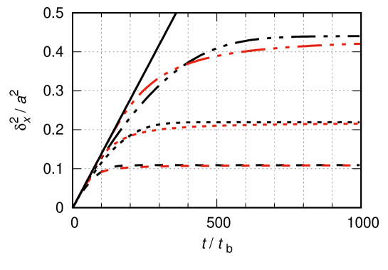
Figure 2: Quantum dynamical time evolution of the mean square displacement (MSD) $\delta_{x}^{2}(t)$ of a CO molecule ($m\approx 28$ u) moving on a hypothetically flat Cu(100) surface ($a\approx 256$ pm) at a temperature $T=190$ K. Black interrupted lines show the MSD for quasi-ideal particles according to Eq. (9) for finite values of $L$: $L=10\,a$ (     ), $L=20\,a$ (       ), $L=40\,a$ (       ). The continuous black line is for $L\to\infty$ (ideal particle, Eq. (13)). The red interrupted lines give results from Eq. (22) with an optimized parameter $\alpha=0.35$. The time unit is $\mbox{$t_{\rm b}$}=\hbar\beta\approx 40$ fs.

Initially, the MSD of the quasi-ideal and ideal particles match. The larger $L$, the longer is the agreement. For very short times of order $t_{\rm b}$, because $\sin((E_{n}-E_{j})t/2\hbar)\approx(E_{n}-E_{j})t/2\hbar$, $\delta_{x}^{2}(t)\propto t^{2}$ holds also from the numerical evaluation of Eq. (9).

For $t\to\infty$ the MSD for the quasi-ideal particle stagnates asymptotically forming a plateau which is also its upper bound. The positions of the plateaus increase linearly with the super-cell length. They furthermore agree perfectly with the values $\breve{\delta}_{x}^{2}(L=10\,a)\approx 0.11\,a^{2}$, $\breve{\delta}_{x}^{2}(L=20\,a)\approx 0.22\,a^{2}$ and $\breve{\delta}_{x}^{2}(L=40\,a)\approx 0.44\,a^{2}$ from Eq. (16). Quite remarkably, the asymptotic MSD is only a fraction of the area $a^{2}$ of a primitive cell, even for super-cells 40 times larger. Boundary effects therefore influence the MSD evolution rather dramatically. The low asymptotic bound of the MSD must be related to the extremely high degree of delocalization of the thermal wave packet underlying Eq. (9) throughout the super-cell, and a corresponding small thermal de Broglie wave length, as discussed below. The delocalization enhances the boundary effects.

The time evolution of the MSD for a quasi-ideal particle shows the characteristic pattern of a confined diffusion Jardine et al. (2009), or of the diffusion in a Debye crystal Chudley and Elliot (1961). Here, it can be understood in terms of the statistical model outlined in section II.4, as shown by the red interrupted lines in Figure 2 which reproduce the function $\left\langle{\delta}_{x}^{2}\right\rangle_{v}(t)$ defined by Eq. (22), for different values of the super-cell length $L$, and capture well the behavior of $\delta_{x}^{2}(t)$ when the value $\alpha=0.35$ is assumed for all values of $L$. The good qualitative agreement between the black and red interrupted lines supports the physical interpretation underlying the model, in that the boundary conditions for thermalized states effectively reflect collisions and decoherence. No quantitative agreement should be expected from this rather simple interpretation, however. Addressing its reality is much beyond the scope of the present work. The model just underlines that the independent particle picture adopted here for the evaluation of the MSD looses its legitimacy after some time and that a more realistic simulation of the evolution of the MSD beyond that time would need interactions among particles somehow to be included, which would lead to much more involved quantum master equations such as in ref. 29.

IV Conclusions

The mean square displacement (MSD) $\delta_{x}^{2}(t)$ of a particle of mass $m$ at thermal equilibrium with its environment is an important quantity in atomic and molecular physics, as well as in transport phenomena. While this quantity emerges naturally from classical statistical mechanics, the search for a corresponding quantum mechanical expression has not been carried out sufficiently far, to the best of our knowledge. At thermal equilibrium, when the ensemble averaged view of the density matrix is adopted, any observable is a constant of time, and the MSD vanishes identically. A different result is obtained, when the view is taken up that the thermal state of the particle is described by a typical member of the statistical ensemble.

From this prospective, a general expression for the MSD of a thermalized particle moving independently in a one dimensional, periodic potential $V(x)$ is proposed in Eq. (9) in terms of the eigenstates and eigenvalues of the particle in that potential, and temperature. It is a key aspect of the formalism that a thermal state of the particle is described by a typical member of the thermal ensemble, rather than by its statistical average. As a consequence, the probability density shows fluctuations which are essential to obtain quantum mechanically a time dependent MSD. In the case of a free moving particle in an infinitely large space, $V\equiv 0$, Eq. (9) yields the simple analytical formula in Eq. (13) for what was termed the MSD of an ideal particle.

Eq. (13) reveals an interesting behavior: while initially of ballistic character, the MSD of the ideal quantum particle of mass $m$ moving in an unrestrained manner at temperature $T$ gains the character of a Brownian diffusion after a time of order $\mbox{$t_{\rm b}$}\equiv\hbar/(\mbox{$k_{\rm B}$}\,T)$. The temperature independent slope of the MSD obtained at long times is given by $\mbox{$D_{\rm q}$}=\hbar/(2\,d\,m)$, where $d$ is the dimensionality of the particle. Although $D_{\rm q}$ has the dimension of a diffusion coefficient, these quantities should probably not be related as such in the classical understanding of diffusion, due to the absence of friction in the present theoretical framework.

Albeit interesting, this result also irritates, as it marks a stark difference between the classical (ballistic) and quantum (Brownian diffusion) behavior of the MSD for the ideal, thermalized particle. Because $\delta_{x}^{2}(t)$ vanishes identically in the limit $\hbar\to 0$, this quantity should be considered as having no classical counterpart. It was nevertheless shown analytically, how the quantum mechanical MSD of an ideal particle can in principle be extracted from helium-3 spin echo experiments by the measurement of the phase $\phi_{\rm ISF}$ of the intermediate scattering function (ISF). For real particles, neither the quantum mechanical MSD nor the ISF are known analytically. The MSD can be obtained numerically from Eq. (9). The relation between $\phi_{\rm ISF}$ and the MSD remains hypothetical and worth an experimental verification.

In numerical evaluations with periodic boundary conditions the MSD for a free particle initially overlaps with the analytical result but then evolves asymptotically into a plateau which defines its upper bound. The longer the periodically repeated cell, the higher is the asymptotic value. This value equals the value the MSD would have gained if, in the course of its free evolution, the particle had undergone a collision or any other interaction leading to a decoherence of its density matrix. A simple model based on statistically distributed collision times allows one to describe qualitatively the numerical result and to interpret the onset of the plateau as resulting from a decoherence that is effectively generated by the boundary conditions. To verify the truthfulness of this interpretation, real many body interactions need to be considered in a significantly more involved open system treatment of the dynamics, which is beyond the scope of the present work.

The present investigation is planed to be extended to a full dimensional treatment of the dynamics including interactions between the particles and global potential energy surface calculated from ab initio calculations, for instance for the motion of carbon monoxide molecules adsorbed on a copper substrate Marquardt et al. (2010). Inspired by previous work, inclusion of substrate atoms in the dynamics in an explicit way Meng and Meyer (2017), in a hierarchical effective mode approach Burghardt et al. (2012), or in the form of stochastic operators Serwatka and Tremblay (2019) will allow us to address more precisely the role of friction on the specific dynamics of CO on Cu(100) from first principle calculations. Potentially, non-adiabatic couplings will also need to be considered, although for CO on Cu(100) they should play a minor role. Theoretical results can be expected to become full quantitative once these additional effects have been considered, which should ultimately allow us to verify the method and to assess the quality of the potential energy surfaces calculated ab initio. To this end, the present work delivers an important technical information by showing that the quantum dynamical simulation of the long time evolution of a thermal state of the adsorbate requires large grids corresponding to low coverage degrees of the substrate.

Accurate theoretical simulations of the diffusion of adsorbates on substrates are important tools to increase our knowledge of this process. The present investigation has shown that some essential properties of diffusion emerge naturally and quite realistically in a quantum mechanical description of the adsorbates’ dynamics. Scanning tunneling microscopy (STM) allows one to measure diffusion rates at the single atom level Briner et al. (1997); Lauhon and Ho (2002); Bartels et al. (2004). STM would therefore be ideally suitable to measure the mean square displacement of xenon atoms on platinum and to discriminate whether they move as classical or quantum particles. With these techniques the question arises, however, as to what extent the STM apparatus does not itself influence the motion of the adsorbed species Ternes et al. (2008); Nacci et al. (2018). It will be interesting to address this question in the context of a full quantum mechanical simulation of the STM experiment that includes the motion of the adsorbates.

Appendix A Free particle

We first consider a super-cell of length $L$ with basis functions $\phi_{n}(x)=\mbox{$\langle{x}\rvert{\phi_{n}}\rangle$}={\rm e}^{\displaystyle-\mbox{{$\rm i$}}q_{n}x}/\sqrt{L}$, where $n\in\mathbb{Z}$, and $q_{n}=n2\pi/L=p_{n}/\hbar$, where $p_{n}$ is the momentum of the system in state $\lvert{\phi_{n}}\rangle$. For a free particle of mass $m$, $V(x)\equiv 0$, and these states are eigenstates of the Hamiltonian of Eq. (2) with eigenvalues $E_{n}=p_{n}^{2}/2m=\hbar^{2}q_{n}^{2}/2m$.

The matrix elements $x_{nj}=\mbox{$\langle{\phi_{n}}\rvert$}\hat{x}\mbox{$\lvert{\phi_{j}}\rangle$}$ can be expressed analytically:

$$x_{nj} = \mbox{{$\rm i$}}\,\left(\frac{2\,\sin((q_{n}-q_{j})\,L/2)}{L\,(q_{n}-q_{j})^{2}}\;-\;\frac{\cos((q_{n}-q_{j})\,L/2)}{q_{n}-q_{j}}\right)$$ (A1)

Note that $x_{nn}$ exists and yields exactly $x_{nn}=0$. Because $q_{n}=2\pi\,n\,/\,L$, these matrix elements simplify:

$$x_{nj} = \left\{\begin{array}[]{lr}0&n=j\\ \mbox{{$\rm i$}}\,\frac{\displaystyle(-1)^{n-j+1}}{\displaystyle q_{n}-q_{j}}&n\neq j\end{array}\right.$$ (A4)

Insertion in Eq. (9) yields

$$\delta_{x}^{2}(t) = \frac{4}{Q^{2}}\;{\sum\limits_{n=-\infty}^{\infty}}^{\prime}{\sum\limits_{j=-\infty}^{\infty}}^{\prime}{\rm e}^{\displaystyle-\beta\,\hbar^{2}\,(q_{n}^{2}+q_{j}^{2})/(2m)}\;\frac{\sin^{2}\left[(q_{n}^{2}-q_{j}^{2})\,\hbar t\,/\,(4m)\right]}{(q_{n}-q_{j})^{2}}$$ (A5)

Here the sums extend from $-\infty$ to $+\infty$, and a state with energy $E_{n}$ is doubly degenerate for $n\neq 0$. In these sums, the combination $n=j$ is explicitly discarded, which is indicated by the prime symbols.

The sums can be replaced by Riemann sums and, approximately, by the integrals:

$$\delta_{x}^{2}(t) \approx \frac{4}{Q^{2}}\,\frac{L^{2}}{4\pi^{2}}\;{\int\limits_{-\infty}^{\infty}\,}^{\prime}\,\mbox{\rm d}{q}\;{\int\limits_{-\infty}^{\infty}\,}^{\prime}\,\mbox{\rm d}{q^{\prime}}\;{\rm e}^{\displaystyle-\beta\hbar^{2}/(2m)\,(q^{2}+{q^{\prime}}^{2})}\;\frac{\sin^{2}\left[(q^{2}-{q^{\prime}}^{2})\,\hbar t\,/\,(4m)\right]\;}{(q-q^{\prime})^{2}}$$

$$= \frac{L^{2}}{2\,\pi^{2}\,Q^{2}}\;\int\limits_{-\infty}^{\infty}\,\mbox{\rm d}{u}\;\mathchoice{{\vbox{\hbox{$\textstyle-$}}\kern-5.34723pt}}{{\vbox{\hbox{$\scriptstyle-$}}\kern-3.57503pt}}{{\vbox{\hbox{$\scriptscriptstyle-$}}\kern-2.52084pt}}{{\vbox{\hbox{$\scriptscriptstyle-$}}\kern-2.0625pt}}\!\int\limits_{-\infty}^{\infty}\,\mbox{\rm d}{v}\;{\rm e}^{\displaystyle-\beta\hbar^{2}/(2\,m\,L^{2})\,(u^{2}+v^{2})}\;\frac{\sin^{2}[\hbar\,u\,\,v\,t\,/\,(2\,m\,L^{2})]}{v^{2}}$$

(A6)

The prime symbols keep the same signification. In the second equation, the variable substitutions $u=(q+q^{\prime})L/\sqrt{2}$ and $v=(q-q^{\prime})L/\sqrt{2}$ were adopted and the integral over $v$ is understood as the principal value (symbol $\mathchoice{{\vbox{\hbox{$\textstyle-$}}\kern-5.34723pt}}{{\vbox{\hbox{$\scriptstyle-$}}\kern-3.57503pt}}{{\vbox{\hbox{$\scriptscriptstyle-$}}\kern-2.52084pt}}{{\vbox{\hbox{$\scriptscriptstyle-$}}\kern-2.0625pt}}\!\int$). The replacement of the sums by Riemann integrals invariably leads to errors. Their relevance will be discussed in detail below.

The two integrals can be evaluated separately. The integral over $u$ yields

$$F(v,t) = \int\limits_{-\infty}^{\infty}\;{\rm e}^{\displaystyle-\beta\hbar^{2}/(2mL^{2})\,u^{2}}\,\sin^{2}\left(\frac{\hbar\,v\,t}{2\,m\,L^{2}}\,u\right)\;\mbox{\rm d}{u}$$ (A7)

$$= \sqrt{\frac{\pi\,m}{2\,\beta\,\hbar^{2}}}\,L\;\left(1-{\rm e}^{\displaystyle-\frac{\displaystyle t^{2}}{2\beta\,m\,L^{2}}\,v^{2}}\right)$$

Consider the two characteristic times: $\mbox{$t_{\rm c}$}=\sqrt{\beta\,m}\,L$ and $\mbox{$t_{\rm b}$}=\hbar\beta$. Then the function $F(v,t)$ can be expressed as

$$F(v,t) = \sqrt{\frac{\pi}{2}}\,\frac{\mbox{$t_{\rm c}$}}{\mbox{$t_{\rm b}$}}\;\left(1-{\rm e}^{\displaystyle-\frac{\displaystyle t^{2}}{2\,\mbox{$t_{\rm c}$}^{2}}\,v^{2}}\right)$$ (A8)

Note that, in the limit $L\to\infty$, the following expressions hold for the partition function:

$$Q = \sum\limits_{n=-\infty}^{\infty}\,{\rm e}^{\displaystyle-\beta\,E_{n}}=\sum\limits_{n=-\infty}^{\infty}\,{\rm e}^{\displaystyle-\beta\,\hbar^{2}\,q_{n}^{2}/(2m)}$$ (A9)

$$\approx \frac{L}{2\pi}\;\int\limits_{-\infty}^{\infty}\;{\rm e}^{\displaystyle-\beta\hbar^{2}/(2m)\;q^{2}}\;\mbox{\rm d}{q}=L\;\sqrt{\frac{m}{2\pi\beta\hbar^{2}}}$$

$$= \frac{1}{2\pi}\;\frac{L}{\lambda_{T}}=\frac{1}{\sqrt{2\pi}}\;\frac{\mbox{$t_{\rm c}$}}{\mbox{$t_{\rm b}$}}$$

The MSD is then approximately given by the integral over $v$:

$$\delta_{x}^{2}(t) \approx \frac{L^{2}}{2\pi^{2}\,Q^{2}}\;\mathchoice{{\vbox{\hbox{$\textstyle-$}}\kern-5.34723pt}}{{\vbox{\hbox{$\scriptstyle-$}}\kern-3.57503pt}}{{\vbox{\hbox{$\scriptscriptstyle-$}}\kern-2.52084pt}}{{\vbox{\hbox{$\scriptscriptstyle-$}}\kern-2.0625pt}}\!\int\limits_{-\infty}^{\infty}\,\mbox{\rm d}{v}\;{\rm e}^{\displaystyle-\beta\hbar^{2}/(2mL^{2})\,v^{2}}\,\frac{F(v,t)}{v^{2}}$$ (A10)

$$\approx L^{2}\,\sqrt{\frac{2}{\pi}}\,\frac{\mbox{$t_{\rm b}$}}{\mbox{$t_{\rm c}$}}\;\mathchoice{{\vbox{\hbox{$\textstyle-$}}\kern-5.34723pt}}{{\vbox{\hbox{$\scriptstyle-$}}\kern-3.57503pt}}{{\vbox{\hbox{$\scriptscriptstyle-$}}\kern-2.52084pt}}{{\vbox{\hbox{$\scriptscriptstyle-$}}\kern-2.0625pt}}\!\int\limits_{0}^{\infty}\,\mbox{\rm d}{v}\;{\rm e}^{\displaystyle-\frac{\displaystyle\mbox{$t_{\rm b}$}^{2}}{\displaystyle 2\,\mbox{$t_{\rm c}$}^{2}}\,v^{2}}\,\frac{1-{\rm e}^{\displaystyle-\frac{\displaystyle t^{2}}{2\,\mbox{$t_{\rm c}$}^{2}}\,v^{2}}}{\displaystyle v^{2}}$$

In the last equation we used the fact that the integrand is an even function of $v$.

For $\infty>a\geq 0$ and $b>0$, the integral

$$I(a,b) = \int\limits_{0}^{\infty}\;{\rm e}^{\displaystyle-b\,x^{2}}\,\frac{1-{\rm e}^{\displaystyle-a\,x^{2}}}{x^{2}}\;\mbox{\rm d}{x}$$ (A11)

has an integrable singularity at $x=0$, so that the principal value exists. An analytical expression for it can be readily obtained:

$$I(a,b) = \sqrt{\pi}\,\left(\sqrt{a+b}-\sqrt{b}\right)$$ (A12)

While the principal value undoubtedly exists for $a=0$, the result shows that for $a\to\infty$, the integral diverges. The assessment of the error made by substituting the Riemann sums by integrals presented in the next section gives further insight.

In terms of $I(a,b)$, with $a=t^{2}/(2\mbox{$t_{\rm c}$}^{2})$ and $b=\mbox{$t_{\rm b}$}^{2}/(2\mbox{$t_{\rm c}$}^{2})$, the MSD is then expressed as

$$\delta_{x}^{2}(t) \approx L^{2}\,\sqrt{\frac{2}{\pi}}\,\frac{\mbox{$t_{\rm b}$}}{\mbox{$t_{\rm c}$}}\;\sqrt{\pi}\;\left(\sqrt{\frac{t^{2}}{2\,\mbox{$t_{\rm c}$}^{2}}+\frac{\mbox{$t_{\rm b}$}^{2}}{2\,\mbox{$t_{\rm c}$}^{2}}}-\sqrt{\frac{\mbox{$t_{\rm b}$}^{2}}{2\,\mbox{$t_{\rm c}$}^{2}}}\right)=L^{2}\;\frac{\mbox{$t_{\rm b}$}^{2}}{\mbox{$t_{\rm c}$}^{2}}\;\left(\sqrt{\frac{t^{2}}{\mbox{$t_{\rm b}$}^{2}}+1}-1\right)$$ (A13)

$$= \frac{\mbox{$t_{\rm b}$}^{2}}{\beta\,m}\;\left(\sqrt{\frac{t^{2}}{\mbox{$t_{\rm b}$}^{2}}+1}-1\right)=\underbrace{\frac{\mbox{$t_{\rm b}$}}{\beta\,m}}_{\displaystyle\hbar/m}\;\left(\sqrt{t^{2}+\mbox{$t_{\rm b}$}^{2}}-\mbox{$t_{\rm b}$}\right)$$

This is Eq. (13). In two dimensions, because the total square displacement is the sum of the square displacements in two orthogonal directions, the result is to be multiplied by the factor two. Similarly, in three dimensions, the factor three applies.

Despite the fact that the result is independent of $L$, Eq. (A13) is an approximation to the sum in Eq. (A5) (and Eq. (9)) that becomes better, the larger $L$. Nevertheless, the error can diverge for $t\to\infty$ and any finite value of $L$, as discussed in the following.

Appendix B Free particle, error estimation and a closed formula for $\breve{\delta}_{x}^{2}$

The main cause of error between Eqs. (A13) and (A5) is due to the evaluation of the integral in Eq. (A11). Let

$$f(x,a)=\frac{1-{\rm e}^{\displaystyle-a\,x^{2}}}{x^{2}}$$ (B14)

where $x,a\in\mathbb{R}^{+}$. Let $x_{n}=n\,\Delta x$, with $n=1,2,\ldots$ and $\Delta x>0$. For sufficiently small $\Delta x$, $\int_{0}^{\infty}\,f(x,a)\,\mbox{\rm d}{x}=\sum_{n=1}^{\infty}\,f(x_{n})\,\Delta x+O(\lvert f^{\prime\prime}\rvert\,(\Delta x)^{3})$. The function $f^{\prime\prime}$ has an extremum at $x=0$: $\max(\lvert f^{\prime\prime}\rvert)=a^{2}/2$. With $a=(t/\mbox{$t_{\rm c}$})^{2}/2$, the error will hence evolve as $t^{4}(\Delta x)^{3}$. This evolution is clearly illustrated in Figure 2 in the main part of the text.

Yet, Eq. (A11) suggests that $I(a\to\infty,b)=\int_{0}^{\infty}\,{\rm e}^{\displaystyle-b\,x^{2}}/x^{2}\,\mbox{\rm d}{x}$ is related to the asymptotic value $\delta_{x}^{2}(t\to\infty)$, which is finite for finite values of $L$, as shown in Figure 2. In the following a closed analytical formula is developed for this quantity.

From Eq. (A7), $F(v,t\to\infty)=\sqrt{\pi\,m/(2\,\beta\,\hbar^{2})}\,L$, which can be obtained by replacing $\sin^{2}[\hbar\,u\,v\,t\,/\,(2\,m\,L^{2})]\equiv 1/2$ in Eq. (A6) and, consequently, in Eq. (A5). Upon replacement, the resulting sum is exactly the expression for $\breve{\delta}_{x}^{2}$ in Eq. (12).

In order to obtain a closed formula for this quantity, we use the definition for the matrix elements of the position operator given in Eq. (A1), i.e. we consider

$$\breve{\delta}_{x}^{2} = \frac{2}{Q^{2}}\;{\sum\limits_{n=-\infty}^{\infty}}^{\prime}{\sum\limits_{j=-\infty}^{\infty}}^{\prime}{\rm e}^{\displaystyle-\beta\,\hbar^{2}\,(q_{n}^{2}+q_{j}^{2})/(2m)}\;X^{2}(q_{n}-q_{j})$$ (B15)

where

$$X(q) = L\,\left(\frac{2\,\sin(L\,q/2)}{L^{2}\,q^{2}}\;-\;\frac{\cos(L\,q/2)}{L\,q}\right)$$ (B16)

Because $q_{n}=2\pi\,n\,/\,L$, $X(q_{n}-q_{j})^{2}=1/(q_{n}-q_{j})^{2}=\lvert x_{nj}\rvert^{2}$. This change will not alter the result expected for the sum in Eq. (12). However, it will change the behavior of the corresponding Riemann integral. It leads to the replacement of the integral in Eq. (A11) by $J(b)-J(a+b)$, where

$$J(y) = 2\,\int\limits_{0}^{\infty}\;{\rm e}^{\displaystyle-y\,x^{2}}\,\;\left(\frac{\sin(x/\sqrt{2})}{x^{2}}-\frac{\cos(x/\sqrt{2})}{\sqrt{2}\,x}\right)^{\displaystyle 2}\;\mbox{\rm d}{x}$$ (B17)

This integral can be solved analytically and yields Eq. (LABEL:Jy). The error function $\mbox{{$\rm erf$}}(x)$ is defined as

$$\mbox{{$\rm erf$}}(x)=\frac{2}{\sqrt{\pi}}\,\int\limits_{-\infty}^{x}\,{\rm e}^{\displaystyle-y^{2}}\;\mbox{\rm d}{y}-1$$ (B18)

Because $\mbox{{$\rm erf$}}(\infty)=1$, $\mbox{{$\rm erf$}}(0)=0$ and $\lim\limits_{y\to\infty}(1-\exp(-1/(2y)))y=1/2$

$$J(0) = \frac{\sqrt{2}\pi}{12}$$ (B19)

$$J(\infty) = 0$$ (B20)

Consequently, we may write

$$\breve{\delta}_{x}^{2} \approx L^{2}\,\sqrt{\frac{2}{\pi}}\,\frac{\mbox{$t_{\rm b}$}}{\mbox{$t_{\rm c}$}}\;J\left(\frac{1}{2}\left(\frac{\mbox{$t_{\rm b}$}}{\mbox{$t_{\rm c}$}}\right)^{2}\right)$$ (B21)

$$= L\,\hbar\,\sqrt{\frac{2\,\beta}{\pi\,m}}\;J\left(\frac{\hbar^{2}\,\beta}{2\,m\,L^{2}}\right)$$

For $L\to\infty$, this quantity scales with $L$ and not with $L^{2}$, as could have been expected.

The error made in approximating the Riemann sum by integrals can be assessed via the function

$$\tilde{f}(x,a)=\left(1-{\rm e}^{\displaystyle-a\,x^{2}}\right)\;\left(\frac{\sin(x/\sqrt{2})}{x^{2}}-\frac{\cos(x/\sqrt{2})}{\sqrt{2}\,x}\right)^{\displaystyle 2}$$ (B22)

The second derivative of this function can be given as $\tilde{f}^{\prime\prime}(x,a)=c_{1}(x,a)\,{\rm e}^{\displaystyle-a\,x^{2}}+c_{2}(x)$, where $c_{1}$ and $c_{2}$ are analytical and bound on the real axis (for both $x$ and $a$). In the limit $a\to\infty$ (corresponding to $t\to\infty$), the error is therefore of order $\lvert c_{2}(x)\rvert\,(\Delta x)^{3}$, which is convergent.