Computing Shapley Effects for Sensitivity Analysis

Abstract

Shapley effects are attracting increasing attention as sensitivity measures. When the value function is the conditional variance, they account for the individual and higher order effects of a model input. They are also well defined under model input dependence. However, one of the issues associated with their use is computational cost. We present a new algorithm that offers major improvements for the computation of Shapley effects, reducing computational burden by several orders of magnitude (from $k!\cdot k$ to $2^{k}$, where $k$ is the number of inputs) with respect to currently available implementations. The algorithm works in the presence of input dependencies. The algorithm also makes it possible to estimate all generalized (Shapley-Owen) effects for interactions.

1 Introduction

Computer experiments are widely adopted in modern scientific investigations to simulate natural, social and physical phenomena. The increase in computing power allows analysts to develop simulators of increasing complexity and analytical approaches fail in delivering insights about the simulator behavior. Thus, the input-output relationship is often considered as a black-box.

Sensitivity analysis allows us to shed light on the structure of a black-box model, providing the modelers with insights useful in building and interpreting simulator results [34]. A major concern of computer modelers is the quantification of the relative importance of the inputs of the codes. When the model inputs are uncertain, this task is typically performed using global sensitivity analysis methods. One can find alternative global sensitivity analysis approaches, including variance-based [34], regression-based [37] and moment-independent sensitivity methods [3].

In the computer experiments literature, Shapley values are enjoying an increasing popularity (see, e.g., [2, 14, 27, 29] for recent contributions to theory and applications). Shapley values originate from game theory [35] and are based on the allocation of the total value of a game to the contribution of each player. In the context of sensitivity analysis, Shapley values have been proposed for the first time in [23] and called Shapley effects. The intuition is to regard model inputs as players and the conditional variance they explain as the value function. One main reason for the interest towards Shapley effects is that they remain interpretable also in the presence of dependent inputs [36, 24, 14] or domain irregularities such as holes [24]. In such cases, these importance indices never become negative [24].

However, the computation of Shapley effects can be very demanding. A seminal proposal can be found in [36]. The work suggests a fourfold algorithm: Looping over all permutations (or a randomly selected subset [8]), looping over the path through a hypercube of index subsets induced by that permutation, looping over an outer and inner loop for obtaining conditional variances, switching inputs on and off along that path to compute the sum of marginal contributions. In [7] the algorithm is improved by using pick’n’freeze sampling and ignoring high-order terms in presence of block-independent group of variables. In [6] an algorithm based on nearest neighbor estimators of the marginal contributions is proposed.

In this paper, we offer an alternative algorithm. We proceed in two steps. First, we examine a series of refinements of the current implementation of [36] with the goal of achieving memory and time savings. Then, we change the logic for computing Shapley effects by switching from permutations of marginal effects to using Möbius inverses. This restructuring decreases computational cost from $k!\cdot k$ to $2^{k}$ evaluations of a basic sample block, where $k$ is the number of model inputs.

We challenge the algorithm through several experiments, comparing its performance against that of previously available algorithms. The experiments show that the proposed implementation leads to the following advantages. The algorithm reduces computational burden notably (is memory and time-wise faster than the currently published predecessors), leads to unbiased estimates, allows the possibility of computing both Shapley effects and Shapley-Owen interaction effects. These latter indices are a generalization of Shapley effects introduced in [28] to study the synergistic/antagonistic nature of interactions among inputs. We remark that the algorithms of [36, 6] to compute Shapley effects don’t allow one to estimate the Shapley-Owen interaction effects. In fact, these two algorithms are based on the permutation representation of Shapley effects, which is not available at the moment for the Shapley-Owen effects.

This paper is structured as follows. Section 2 presents the concept of Shapley value from game theory. Section 3 presents the Shapley effects for global sensitivity analysis. Section 4 presents an improvement of the algorithm of [36]. The new Möbius inverse-based algorithm is presented in Section 5. Section 6 contains the numerical experiments.

2 Shapley Value

The Shapley value [35] is a concept from cooperative game theory. One considers a game with $k$ players. The Shapley value is then the quantity that indicates the worth of forming coalitions and the expected payoff for each player. Generally, one defines the coalition worth function $\operatorname{val}:2^{\underline{k}}\to\mathbb{R}_{\geq 0}$ with $\operatorname{val}(\emptyset)=0$, attributing a sum of payoffs to a group of players. Here $2^{\underline{k}}$ is the powerset (set of subsets) of $\underline{k}=\{1,2,\dots,k\}$.

Definition 1.

Given a coalition worth function $\operatorname{val}$, the marginal contribution of player $i$ joining coalition $\alpha$ is $\operatorname{mar}(\alpha,i)=\operatorname{val}(\alpha\cup\{i\})-\operatorname{val}(\alpha)$.

The Shapley value is then defined by

(1) $$\begin{split}\Phi_{i}(\operatorname{val}{})&=\sum_{\alpha:i\not\in\alpha}\frac{\left\lvert\alpha\right\rvert!(k-\left\lvert\alpha\right\rvert-1)!}{k!}\left(\operatorname{val}(\alpha\cup\{i\})-\operatorname{val}(\alpha)\right)\\ &=\frac{1}{k}\sum_{\alpha:i\not\in\alpha}{\binom{k-1}{\left\lvert\alpha\right\rvert}}^{-1}\operatorname{mar}(\alpha,i).\end{split}$$

Proposition 2.

The Shapley value of player $i$ is characterized by the following four axioms,

• Pareto-efficiency: $\sum_{i=1}^{k}\Phi_{i}(\operatorname{val}{})=\operatorname{val}(\underline{k})$

• Symmetry: If $\operatorname{val}(\alpha\cup\{i\})=\operatorname{val}(\alpha\cup\{j\})$ for all subsets $\alpha$ containing neither $i$ nor $j$ then $\Phi_{i}(\operatorname{val}{})=\Phi_{j}(\operatorname{val}{})$

• Linearity: $\Phi_{i}(\operatorname{val}_{1}+\operatorname{val}_{2})=\Phi_{i}(\operatorname{val}_{1})+\Phi_{i}(\operatorname{val}_{2})$

• Null-player: If for all $\alpha$, $\operatorname{mar}(\alpha,i)=0$ holds then $\Phi_{i}(\operatorname{val})=0$.

One can interpret the Shapley value either as payoff from joining a coalition or from leaving the anti-coalition. An alternative route to computation is offered by the formula of [10, 23], for which one needs to calculate the Möbius inverses $\operatorname{mob}(\alpha)$ of the value functions $\operatorname{val}(\alpha)$. These are defined implicitly by $\operatorname{val}(\alpha)=\sum_{\beta\subseteq\alpha}\operatorname{mob}(\beta)$ and therefore $\operatorname{mob}(\alpha)=\sum_{\beta\subseteq\alpha}(-1)^{\left\lvert\alpha\right\rvert+\left\lvert\beta\right\rvert}\operatorname{val}(\beta)$ [21, Chap. 8], [30]. Then

(2) $$\Phi_{i}(\operatorname{val}{})=\sum_{\alpha:i\in\alpha}\frac{\operatorname{mob}(\alpha)}{|\alpha|}.$$

Hence each Möbius inverse is weighted by the number of members in the coalition: Player $i$ gets full credit for the games won by one-self, half credit for those were the player teamed up in pairs, etc.

3 Shapley Effects for Sensitivity Analysis

In sensitivity analysis, one usually asks the question of the extent with which an uncertain input influences the outcome of a complex simulation code [4]. Hence, the role of the players is taken by the inputs and $k$ is the input dimension of the simulation model $g:\mathbb{R}^{k}\to\mathbb{R}$.

For sensitivity analysis, the coalition-worth function is taken to be the variance of conditional expectation of $Y$ given $X_{i}$ or the ratio between this quantity and the unconditional variance of $Y$, $\operatorname{val}(\alpha)=\mathbb{V}[Y]^{-1}\mathbb{V}[\mathbb{E}[Y|X_{\alpha}]]$ [23, 24] which then accounts for a grand total of one. For these choices of value functions, the term Shapley effects has been coined. The value functions are then equal to the subset importance of [18]. Under input independence, the Möbius inverses coincide with the variance-based first order and higher order Sobol’ effects, e.g. $\operatorname{mob}(\{i,j\})=\operatorname{val}(\{i,j\})-(\operatorname{val}(\{i\})+\operatorname{val}(\{j\}))$ is the contribution to the output variance stemming from the pairwise interaction/second order effect of inputs $i$ and $j$. Also under input independence, as first order effects $S_{i}$ satisfy $S_{i}=\operatorname{val}(\{i\})=\operatorname{mob}(\{i\})$ and total effects satisfy $T_{i}=\sum_{\alpha:i\in\alpha}\operatorname{mob}(\alpha)$ we have $S_{i}\leq\Phi_{i}(\operatorname{val}{})\leq T_{i}$. So the need for computing Shapley effects arises only if the gap between first order and total effects is large or dependences in the input are present. As a consequence from (2) and Pareto-efficiency we observe the following results.

Proposition 3.

Under input independence, the Shapley effect is bounded by the mean of the main effect and the total effect, $\Phi_{i}\leq\frac{1}{2}(S_{i}+T_{i})$. If equality holds then there are no interaction terms of order larger than two involving input $i$. If the sum of all main and total effects equals $2$ then only pairwise interactions may be present in the model.

We also observe that [36] show the following duality result: considering the value function $\operatorname{val}^{\prime}(\alpha)=\mathbb{E}[\mathbb{V}[Y|X_{\sim\alpha}]]$ instead of $\operatorname{val}(\alpha)=\mathbb{V}[\mathbb{E}[Y|X_{\alpha}]]$ leads to the same Shapley effects. Both of these value functions can be estimated from a pick’n’freeze design.

3.1 Shapley Effects for Groups

Recently, [28] introduce a Shapley effect for groups, building upon results by [25] and [11]. The following expression, termed Shapley-Owen effect for the group $\alpha$, parallels (2),

(3) $$\Phi_{\alpha}(\operatorname{val}{})=\sum_{\beta:\alpha\subseteq\beta}\frac{\operatorname{mob}(\beta)}{|\beta|-|\alpha|+1}.$$

Hence, having available the Möbius inverses allows one to obtain these Shapley-Owen effects. Note that they are governed by a slightly different set of axioms than in Prop. 2.

If all Möbius inverses are nonnegative, we can generalize the findings of Prop. 3, as

(4) $$S_{\alpha}=\operatorname{mob}(\alpha)\leq\Phi_{\alpha}(\operatorname{val}{})\leq\sum_{\beta:\alpha\subseteq\beta}\operatorname{mob}(\beta)=\Upsilon_{\alpha}$$

where $\Upsilon_{\alpha}$ is the superset importance measure of [18]. We can further sharpen the upper bound in (4),

(5) $$\Phi_{\alpha}(\operatorname{val}{})\leq\operatorname{mob}(\alpha)+\frac{1}{2}\sum_{\beta:\alpha\subsetneq\beta}\operatorname{mob}(\beta)=\frac{1}{2}\left(\operatorname{mob}(\alpha)+\sum_{\beta:\alpha\subseteq\beta}\operatorname{mob}(\beta)\right).$$

We then formulate an interaction analogon of Proposition 3.

Proposition 4.

Under input independence, the Shapley-Owen effect for input group $\alpha$ is bounded by the mean of the Sobol’ index and the superset importance of $\alpha$, that is $\Phi_{\alpha}\leq\frac{1}{2}(S_{\alpha}+\Upsilon_{\alpha})$. If equality holds then there are no higher order interaction terms larger than $|\alpha|+1$ involving $\alpha$.

4 A Refinement

A first algorithm we study is based on the sample approach of [36], with some marginal modifications aimed at improving estimation accuracy. We propose to:

• Use of a pick’n’freeze design [9, 7] instead of a brute-force double loop to compute conditional variances

• Use of duality result: two estimators can be obtained for the same computational costs

• Estimation of conditional variances via Sobol’/Saltelli and Jansen formulas to take advantage of the pick’n’freeze design and the duality result

• Use of quasi Monte-Carlo (QMC) design for improved convergence [16] compared to a crude Monte-Carlo design

The convergence properties of pick’n’freeze designs are discussed in [9]. Combined with QMC sampling, one profits of the accelerated convergence of the variance estimates for a large class of functions (i. e. those bounded in the sense of Hardy–Krause). Moreover, the pick’n’freeze design allows one to identify dummies exactly, as theoretically expected (null-player property of Prop. 2), eliminating numerical noise stemming from the variability of variance estimates of different samples as in [36]. The Jansen estimator for superset importance and the Sobol’/Saltelli estimator for subset importance offer two different ways of obtaining Shapley effects.

A version ready to test in MatLab or Octave is available in Algorithm 1. The calling convention requires as parameters the dimension of the model $k$, the size of a basic sample block $n$, the simulation model and the transformation from the unit hypercube into the desired marginal distributions. Both the model function and the input space transformation are assumed to be vectorized.

Further optimizations of Algorithm 1 are possible. Specifically, the ways in which indices of model inputs are selected or deselected by traversing all different permutation paths include the same marginal contribution multiple times. Filling a database of coalition worth value functions as one traverses these paths and querying the database before a model evaluation greatly enhances the applicability, especially in higher input dimensions: There are $2^{k}-1$ value functions for a model with input dimension $k$, as opposed to $k!\cdot k$ evaluations of marginal functions when looping over all permutations ($k!\cdot k\gg 2^{k}$). This requires a database query before the model evaluation and an insertion after the computation of a value function.

Furthermore, the direct storage of all permutations might impair performance (MatLab 2018 warns that for 11 dimensions the permutation matrix will occupy more than 3 Gb). Hence, Heap’s algorithm [12] may be used to generate the possible permutations iteratively instead of filling a large matrix with all combinations.

When referring to Algorithm 1 in the reminder, we shall consider the optimized version which implements these two improvements and which is available upon request.

Algorithm 1 A MatLab/Octave Implementation of Shapley Effects (simplified).

⬇

1ction [Shap,Shap2,evals]=shapley(k,n,model,trafo)

2% SHAPLEY Shapley effects.

3u=sobolpoints(n,2*k); % net(sobolset(2*k),n)

4xa=trafo(u(:,1:k));xb=trafo(u(:,k+1:end));

5

6ya=model(xa);yb=model(xb);evals=2*n;

7Shap=zeros(1,k); Shap2=zeros(1,k);

8

9for p=perms(1:k)' % for each column

10val=0; % coalition worth of empty set

11val2=0;

12xi=xa;

13 for q=p'

14 xi(:,q)=xb(:,q); % winding stairs

15 yi=model(xi);evals=evals+n;

16 nval=mean((yi-ya).^2); % superset importance

17 Shap(q)=Shap(q)+nval-val; % marginal contribution

18 val=nval;

19

20 nval2=yb'*(yi-ya); % subset importance

21 Shap2(q)=Shap2(q)+nval2-val2;

22 val2=nval2;

23 end

24end

25Shap=Shap/2/var(yb)/prod(1:k)

26Shap2=Shap2/n/var(yb)/prod(1:k)

Under input dependence, a Rosenblatt transformation [20] is needed in order to compute dependent conditional input realizations of a input group given realizations of the complementary index group. This can be effectively implemented in the Gaussian copula case (rank correlation, normal-to-anything-transformation, Nataf transformation) using the upper-triangular Cholesky roots of the reordered correlation matrix. One might argue that the quasi Monte-Carlo structure is distorted by the Cholesky root and a symmetric matrix root may be more suitable, however, then the triangular structure and hence the Rosenblatt transformation property is lost.

In case of input dependence, the Jansen estimator of superset importance (as implemented in Lines 16–18) becomes invalid because in this design the input blocks for yi and ya of the complementary index set $\sim\alpha$ are not independent. However, the code for the Sobol’/Saltelli estimator (in Lines 20–22) stays valid as yb and ya are using independent inputs. Hence in the dependent case, the duality between using $\operatorname{val}{}$ and $\operatorname{val}^{\prime}{}$ is lost, but only due to the Jansen estimator breaking down. Alternative estimators (as discussed below) are still working. In the next section, we discuss an alternative approach based on an intuition that notably reduces computational burden. The improved algorithm introduced in this section will then be compared against the new algorithm and the original implementation of [36] in a series of experiments in Section 6.

5 Alternative Approach Using the Möbius Inverse

As the Möbius inverses used in (2) are formally equivalent to the functional ANOVA decomposition terms, (2) offers a viable alternative for computing the Shapley effects. Then the $2^{k}-1$ value functions have to be computed and a system of equations using a sparsely populated $(2^{k}-1)\times(2^{k}-1)$ matrix has to be solved. We investigate if this scheme is more attractive than via the computation of all marginals.

Algorithm 2 A MatLab/Octave Implementation of Shapley Effects using Möbius Inverses.

⬇

1ction [Shap,V]=shapleymoebius(k,n,model,trafo)

2% SHAPLEY Shapley effects using Möbius inverse.

3u=sobolpoints(n+1,2*k);u(1,:)=[];

4xa=trafo(u(:,1:k));xb=trafo(u(:,k+1:end));

5ya=model(xa);yb=model(xb);

6

7if(k$\geq$log2(flintmax)), warning('Precision (and patience) may be lost.');end

8l=2^k-1;H=zeros(2,l);sz=zeros(1,l); for i=1:l

9% selection of input subset

10 g=bitand(i,2.^(0:k-1))$\neq$0; % lsb codes first index

11 sz(i)=sum(g); % subset size

12 xi=xa; xi(:,g)=xb(:,g);

13 yi=model(xi);

14 H(:,i)=[mean((yi-ya).^2)/2;(yb'*(yi-ya))/n];

15end

16%% Shapley effects via Möbius Trafo:

17% poset inclusion matrix is Pascal triangle mod 2

18mob=zeros(2,l); sel=1; for i=1:l

19 ii=find(sel);

20 mob(:,i)=(H(:,ii)*(-1).^(sz(i)+sz(ii)'))/sz(i);

21 sel=xor([1,sel],[sel,0]);

22end

23%% Owen/Grabisch formula (weights are already included)

24Shap=ones(2,k); for i=1:k

25 Shap(:,i)=sum(mob(:,logical(bitand(1:l,2^(i-1)))),2);

26end

27%% variance

28V=H(:,end);

Suppose that all $2^{k}-1$ non-vanishing subsets are indexed, $\alpha_{j},j=1,\dots,2^{k}-1$ and the value functions have been gathered in $H_{j}=\operatorname{val}(\alpha_{j})$. Let the matrix $Z$ code the partial ordering,

$$Z_{jl}=\begin{cases}1&\text{if}\quad\alpha_{j}\subseteq\alpha_{l}\\ 0,&\text{otherwise}.\end{cases}$$

Via this coding, subset inclusion becomes a logical implication between the matrix columns: $\alpha_{j}$ is a subset of $\alpha_{l}$ if for all $m$ with $Z_{mj}=1$ it follows that $Z_{ml}=1$. The Möbius inverses are then obtained from $M=HZ^{-1}$ and by (2) the Shapley effect for input $i$ is given by $\Phi_{i}=\sum_{j:i\in\alpha_{j}}\frac{M_{j}}{|\alpha_{j}|}$. Experiments show that this matrix has a relative number of non-zero elements $\left(\frac{3}{4}\right)^{k}$ compared to the total size of $(2^{k}-1)^{2}$. For larger dimensions, despite being sparsely populated, processing this matrix remains out of reach. If the set of all subsets is obtained via binary coding (the least significant bit ($2^{0}$) codes the first index, etc.), then the matrix $Z$ coding the subset inclusion is Pascal’s triangle modulo 2 for which we can construct the columns by an exclusive-or operation. The theoretical details for the binary representation of this Sierpinski gasket are found in [26]. Figure 1 shows the subset order relation: A new input $i$ is considered at the subset indexed by $2^{i}-1$ and stays active for $2^{i}$ subsets.

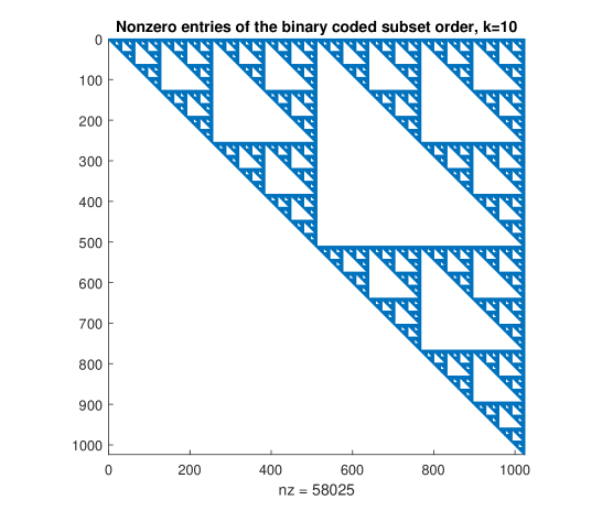
Figure 1: The subset order relation is the Sierpinski gasket, Pascal’s triangle modulo 2.

For inversion we need to determine the signs $(-1)^{|\alpha_{i}|+|\alpha_{j}|}$ from the length of the subsets being compared to one another. The $|\alpha_{i}|$ lengths of the multi-indices are also needed for the weights in (2). Hence we avoid forming and inverting the $Z$ matrix altogether, see line 20 of Algorithm 2, which is a reference implementation. As in Algorithm 1, pick and freeze sampling of quasi Monte-Carlo Sequences as well as both subset and superset importance are used for the computation.

Again, under dependence the Jansen estimator the first component in line 14 of Algorithm 2 is not an estimate of superset importance. Instead, yb’*(yb-yi)/n may be used which estimates the superset importance of the complementary set. The index into the complementary set is then obtained by $2^{k}-1-i$ for $i\neq 2^{k}-1$.

If all the Möbius inverses are available then further sensitivity metrics like effective dimensionality may be computed [2]. Note that both presented algorithms do not take shortcuts by assuming that higher order contributions vanish or by considering a randomized selection of permutations. If the model evaluation takes virtually no time, models with input dimensions up to $k=20$ are computationally tractable with Algorithm 2.

6 Numerical Experiments

In this section, we test Algorithms 1 and 2 and compare their performance with the algorithm of [36] on benchmark analytical models used in previous works on the estimation of Shapley effects. As an application, we consider the fire-spread model studied in [36]. For brevity, we shall use the following abbreviations in this section: EP will refer to the algorithm of [36], based on exact permutations, OP refers to Algorithm 1 including database lookup and iterative generation of permutations, and MI is Algorithm 2 based on Möbius inverses.

6.1 Analytical Models

Let us consider the Ishigami function

$$Y=\sin(X_{1})\left(1+\frac{1}{10}X_{3}^{4}\right)+7\sin(X_{2})^{2},\qquad X_{i}\sim\mathcal{U}(-\pi,\pi),\quad i=1,\dots,4.$$

The inputs are uniformly distributed on $(-\pi,\pi)$. In the analysis we included a dummy input, $X_{4}$. The variance based sensitivity measures of all orders are known for this model [32]: Because the inputs are independent, using [23, Theorem 1] we have the corresponding Shapley effects: $\Phi_{1}=0.4358$, $\Phi_{2}=0.4424$, $\Phi_{3}=0.1218$. Regarding interactions, the only non-vanishing Shapley-Owen effect is $\Phi_{13}=0.2437$.

To estimate the Shapley effects, in OP and MI we use a base sample from a scrambled Sobol’ quasi Monte-Carlo sequence of size 1024. The EP algorithm uses three runs computing conditional variances in the inner MC loop and 64 for the outer loop to estimate the mean of conditional variances, while the unconditional output variance is estimated from a sample of size 1024.

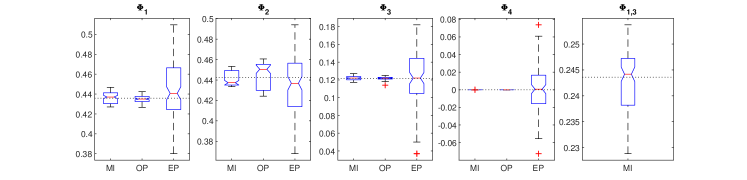
Figure 2: Shapley effects for the Ishigami function. Comparison of MI, OP and EP algorithms. Rightmost graph: Shapley-Owen effect for the pair $(X_{1},X_{3})$.

The results are displayed in Figure 2, showing box-plots of 100 replicates. The analytical values are marked by a dotted line. MI and OP show a comparable performance. The dummy parameter is identified correctly by both algorithms.

Table 1: Ishigami test function with dummy parameter. Details on the computation.

	Möbius Inverse	Optimized Permutations	Exact Permutations
Computational time	5s	2s	2m05s
Model runs	$15360$	$16536$	$14848$
Quadratic Risk	$9.84\cdot 10^{-5}$	$9.05\cdot 10^{-5}$	0.0035

In Table 1 further details are reported. The computational time includes all 100 replicates, while the evaluation count is for a single run of the code. For MI and OP computations where performed in MatLab 2018a, while EP is available from the R sensitivity package. A desktop Windows 7 64 bit machine with i7 processor, 8 Gb RAM was used for the simulations. The number of model evaluations required by the algorithms under comparison is of the same order. The OP algorithm has replaced 82 out to the 98 block model evaluations by a database lookup. As in [6], we also report the quadratic estimation error given by $\sum_{m=1}^{k}\mathbb{E}\left[\left(\hat{\phi}_{m}-\phi_{m}\right)^{2}\right]$ in Table 1.The quadratic risk error term is lower for MI and OP, due to an exact zero for the dummy parameter and also due to the use of a QMC design. The MI algorithm allows one to compute Shapley-Owen effects for groups. We have done so for the only non-vanishing second-order Shapley-Owen effect, which is reported in the rightmost plot of Figure 2.

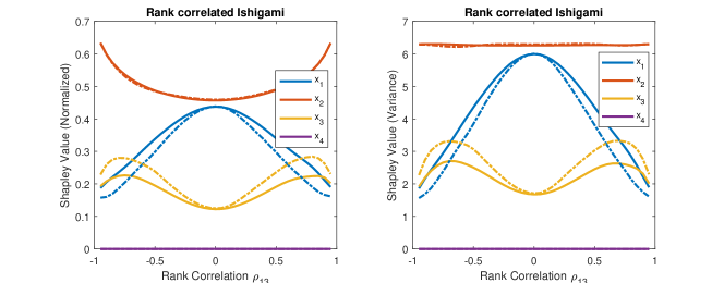
Figure 3: Shapley Effects for the rank-correlated Ishigami function.

For the dependent input case, we introduce a rank correlation between inputs $1$ and $3$ as in [17]. The results for a basic sample block of 1024 are shown in Figure 3. The four lines in Figure 3 represent the Shapley effect of each of the inputs as the correlation between $X_{1}$ and $X_{3}$ varies from $-1$ to $1$. The left graph shows the Shapley effects when the value function is the relative variance contribution, i.e. normalized to one, the right graph when the value function is the absolute variance contribution. The dashed lines are the Shapley effect estimates obtained with the Jansen estimators. As soon as $\rho\neq 0$, these estimates differ from the Sobol’-Saltelli estimates. While the Sobol’-Saltelli estimates are in agreement with the output from the algorithm of [36], the Jansen’s estimates are not. This becomes clear observing that the output from the sample block chosen conditional to the $\alpha$ subset being fixed at positions from the B sample is not the same as the complementary subset $\sim\alpha$ chosen conditionally from the A sample block in the pick’n’freeze estimation scheme under dependence.

Note that one may infer the wrong conclusions when not keeping in mind that the grand total of the output variance may vary: In absolute terms the share attributed to $X_{2}$ does not change, but in relative terms it becomes more important under co- or contramonotonic behaviour of $X_{1}$ and $X_{3}$.

As a second model, we use Sobol $g$ functions. These functions have provided useful test cases for variance-based sensitivity measures [33, 31, 38, 15], but have not been used in the association with Shapley effects yet. We test an $8$ dimensional setting using the parameterization of [33], writing:

$$Y=\prod_{i=1}^{8}\frac{|4X_{i}-2|+a_{i}}{1+a_{i}},$$

where $X_{i}\sim\mathcal{U}[0,1]$ and $a_{1}=a_{2}=0$, $a_{3}=3$, $a_{4}=\cdots=a_{8}=9$. For this model, one can obtain the Shapley effects analytically under independence. The (unnormalized) value functions are $\operatorname{val}{(\alpha)}=\mathbb{V}[\mathbb{E}[Y|X_{\alpha}]]=\prod_{i\in\alpha}(1+V_{i})-1$ where $V_{i}=\mathbb{V}[\mathbb{E}[Y|X_{i}]]=\frac{1}{3}(1+a_{i})^{-2}$ [31, Appendix A]. By [23, Theorem 1], the analytical normalized Shapley effects are $\Phi_{1}=\Phi_{2}=0.469$, $\Phi_{3}=0.0341$, $\Phi_{4,\dots,8}=0.00551$, the estimated values are $\hat{\Phi}_{1}=\hat{\Phi}_{2}=0.48$, $\hat{\Phi}_{3}=0.03$, $\hat{\Phi}_{4,\dots,8}<0.01$. For this estimation, we used MI and OP algorithms with a block sample size of $n=1024$ using QMC. Regarding computational time, OP takes under 10s, while MI takes 0.08s. In terms of numerical results, the behavior is similar to the one registered for the Ishigami function: at $n=1024$, estimates display a negligible numerical error with respect to the analytical values.

It is well known that the number of terms involved in the calculation of Shapley effects increases exponentially with the simulator size. We now consider the 15 dimensional test function presented in [22],

$$Y=g(X)={\left\langle a_{1},\mathbf{X}\right\rangle}+{\left\langle a_{2},\sin(\mathbf{X})\right\rangle}+{\left\langle a_{3},\cos(\mathbf{X})\right\rangle}+{\left\langle\mathbf{X},M\mathbf{X}\right\rangle},$$

where inner products are being formed with prescribed vectors $a_{1}$, $a_{2}$, $a_{3}$ and matrix $M$. The inputs $\mathbf{X}=(X_{1},\dots,X_{15})$ are independently and standard normally distributed. Using a QMC sample of size $2.048$, the MI algorithm takes around 30s, on the same desktop machine as reported before. However, the OP algorithm becomes now time-wise inefficient and does not deliver results in a reasonable amount of time. (In the same time span which MI needed to compute the results, the OP algorithm processed less than $1\%$ of all marginals.)

The normalized Shapley effects obtained with the MI algorithm can be found in Table 2. The Shapley effects are located between the first order and total effects. As the model only has only up to second order interactions, theoretically the Shapley effects should be the mean between first order and total effects (Proposition 3): this can be seen from the sum of both the first order and the total effects being close to $2$.

Table 2: Results for the Oakley/O’Hagan test function, basic sample block 2048 QMC. First and total effects are extracted from the Möbius inverses.

Input	$x_{1}$	$x_{2}$	$x_{3}$	$x_{4}$	$x_{5}$	$x_{6}$	$x_{7}$	$x_{8}$
First order effect	0.0033	-0.0042	0.0010	0.0033	-0.0020	0.0238	0.0287	0.0284
Shapley (subset)	0.0209	0.0327	0.0163	0.0307	0.0105	0.0359	0.0418	0.0560
Shapley (superset)	0.0214	0.0313	0.0202	0.0318	0.0146	0.0347	0.0395	0.0596
Total effect	0.0570	0.0626	0.0360	0.0603	0.0222	0.0394	0.0571	0.0866
Input	$x_{9}$	$x_{10}$	$x_{11}$	$x_{12}$	$x_{13}$	$x_{14}$	$x_{15}$	Sum
First order effect	0.0593	0.0090	0.1078	0.1178	0.1149	0.1030	0.1322	0.7262
Shapley (subset)	0.0837	0.0219	0.1239	0.1232	0.1353	0.1208	0.1464	1.0000
Shapley (superset)	0.0762	0.0239	0.1186	0.1420	0.1238	0.1210	0.1412	1.0000
Total effect	0.1031	0.0364	0.1517	0.1526	0.1444	0.1429	0.1583	1.3105

6.2 Fire-Spread Model

The fire-spread simulator used in [36] is one of the first realistic applications on which algorithms for the estimation of Shapley effects were tested. Other sensitivity analyses of the Rothermel fire-spread model are performed in [19], using a slightly different set of equations than what is discussed here, and in [2]. A state-of-the-art report for this fire-spread simulation model is available as [1]. Starting point of our analysis has been the implementation of the firespread model which can be found at https://EunhyeSong.info/, accessed by the authors on 2019/05/27. The simulator output is the rate of fire-spread and is calculated from the series of equations detailed in Appendix A. As in [36], we consider three distributional scenarios. In the first scenario, model inputs are considered independent (no dependence case). In a second scenario an intermediate level of correlation is introduced between $m_{d}$ and $U$. The rationale is that the windier it is, the dryer the fuel gets. Following the terminology in Song et al. (2016), one calls this the “weak dependence” scenario. In a third scenario, stronger correlations are introduced among the inputs (as per Song et al. 2016, “strong dependence” scenario). Numerically, the “weak dependence” scenario assumes a rank correlation of $-0.3$, the “strong dependence” scenario a rank correlation of $-0.8$.

The inputs and their marginal distributions are listed in Table 3.

Table 3: Fire-spread example: Description of inputs and their marginal distributions. Note that SI units from column 3 are used for describing the probability distributions, while the formulas use imperial units from column 4. The strong wind speed scenario input is already included in the distribution of $U$.

Variable	Description	Units (D)	Units (E)	Distribution	Trunc.
$\delta$	Fuel depth	cm	ft	logn(2.19,.517)
$\sigma$	Fuel particle area to volume ratio	cm-1	ft-1	logn(3.31,.294)	$>\frac{3}{0.6}$
$h$	Fuel particle low heat content	kcal/kg	btu/lb	logn(8.48,.063)
$\rho_{P}$	Oven-dry particle density	g/cm3	lb/ft3	logn(-.592,.219)
$m_{l}$	Moisture content of live fuel	g/g		norm(1.18,.377)	$>0$
$m_{d}$	Moisture content of dead fuel	g/g		norm(.19,.047)
$S_{T}$	Fuel particle total mineral content	g/g		norm(.049,.011)	$>0$
$U$	Wind speed at midflame height	km/h	ft/min	logn(2.9534,.5569)
$\tan\Phi$	Slope			norm(.38,.186)	$>0$
$P$	Dead fuel loading to total fuel loading			logn(-2.19,.66)	$<1$

We propagate uncertainty in the simulator using a quasi Monte-Carlo generator and a sample size of $2^{14}$. Simulation time is $65.5s$ on the aforementioned machine. We note that the fire-spread simulator features a mainly multiplicative input-output mapping. This, together with the choice of logarithmic distributions make the simulator output span several orders of magnitude. In these situations, it has been underlined in previous literature [13, 5] that a slow convergence in variance-based estimators can be expected. Indeed, Figure 4 shows that the first order effects and the total effects differ depending upon using the Jansen or the Sobol’-Saltelli estimators, even for the relative large basic sample size of $2^{14}$. However, despite the fluctuations in variance-based sensitivity measures, the Shapley effects estimates are relatively robust. For the dependent input sample case which postulates two physical plausible scenarios, linking the wind speed and the moisture content together, the duality of the estimators breaks down and we are left with essentially one estimator (the one combining yi with yb).

Under strong dependence the total effect of $m_{d}$ becomes lower than the corresponding first order effect.

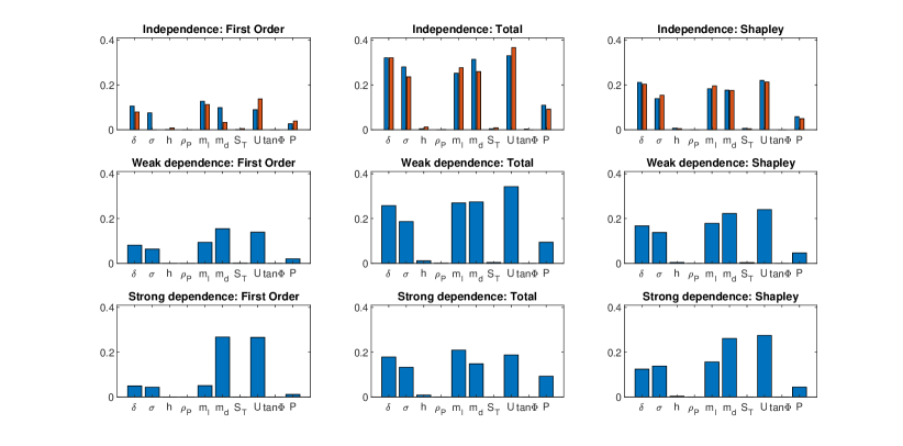
Figure 4: Shapley values for the rank-correlated fire-spread model, basic sample size $2^{14}$.

As mentioned, the algorithm enables the computation of Shapley-Owen interaction effects. Figure 5 reports the pairwise Shapley-Owen effects for the three above mentioned samples, with no dependence ($+$), weak dependence ($\square$) and strong dependence ($\triangleright$). Figure 5 shows that Shapley-Owen effects have absolute values varying from 0 to 0.2, with 30 out of 45 effects null in all three cases of statistical dependence. In the reminder, we shall focus on interactions for which the magnitude of Shapley-Owen effects is higher than 0.01, calling them significant.

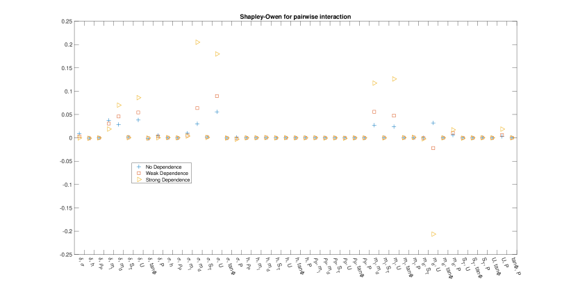
Figure 5: Pairwise Shapley-Owen effects for the rank-correlated fire-spread model.

Input $\delta$ is involved in significant interactions with $m_{l}$, $m_{d}$ and $U$. Input $\sigma$ in turn, is involved in significant interactions with $m_{d}$ and $U$. We then register significant interactions between $m_{l}$ and $m_{d}$, $m_{l}$ and $U$, and between $m_{d}$ and $U$. Note that $h$, $\rho_{P}$ and $\tan\Phi$ show neither Shapley nor Shapley-Owen effects.

As the input correlation increases, a first, overall impression would suggest that the presence of dependence tends to increase the explanatory power of interaction effects. For instance, note the increases in the magnitude of $\phi_{\sigma,m_{d}}$ (from 0.03 to 0.21), of $\phi_{\sigma,U}$ (from $0.055$ to $0.18$). This means that the joint explanatory power of $\sigma$ with $m_{d}$ and with $U$ increases as the correlation among the inputs increases. However, this effect is not systematic. The absolute value of $\phi_{\delta,m_{l}}$ decreases from about $0.04$ in the “no dependence”scenario, to $0.02$ in the “strong dependence”scenario. The Shapley-Owen effect $\phi_{m_{d},U}$ deserves some attention. First, $\phi_{m_{d},U}$ grows in magnitude from 0.03 to 0.21. However, $\phi_{m_{d},U}$ changes sign as we move from the no dependence to the weak dependence and to the strong dependence cases. Thus, these two inputs interact negatively (and strongly negatively) as their negative correlation increases, meaning that they lose explanatory power when considered together. Let us consider the variance-based indices of these two variables. In the no dependence case, their total variance-based indices are greater than they first order indices. In the weak dependence case, the first-order indices are still smaller than the corresponding total ones and the Shapley-Owen effect $\phi_{m_{d},U}$ is now negative but with a small absolute value. In the third case, strong dependence becomes strong, this Shapley-Owen interaction is highly negative and we can see that the total effects for $m_{d}$ and $U$ are lower than their corresponding first-order indices. We also observe that in the strong dependence case, for these two inputs, the bracketing property of [23] doesn’t hold anymore. For instance, we observe the inversion $T_{m_{d}}\leq\Phi_{m_{d}}\leq S_{m_{d}}$. The works [36, 14, 28] discuss other examples of inversion of the bracketing property when inputs become dependent. In this respect, Shapley-Owen effects can offer new insights useful to understand the origin of this inversion.

7 Conclusions

Algorithms for computing Shapley values are attracting increasing interest. In this work, we have proposed an approach based on the Möbius inverse that reduces computational burden notably. The approach enables the computation not only of Shapley effects, but also of Shapley-Owen effects for groups. The algorithm is exact in the sense that all possible input combinations are considered and is valid for all dependent input cases that can to be addressed by Rosenblatt transformations. In terms of future research, we believe that algorithms based on the Möbius-inverse representation of Shapley effects might be beneficial also in the given-data context, for which currently only the permutation-based algorithm of [6] is available. We are currently investigating this possibility.

Appendix A Equations of the Fire-Spread Simulator Used in this Work

The simulator output is given by

(6) $$R =I_{R}\cdot\xi\cdot\frac{1+\Psi_{W}+\Psi_{S}}{\rho_{b}\cdot\epsilon\cdot Q_{\text{ig}}}$$ rate of fire-spread [ft/min]

which is obtained from the following subequations

(7) $$\omega_{0} =\frac{0.2048}{1+\exp\left(\frac{15-30.48\delta}{2}\right)}$$ fuel loading [lb/ft²]

(8) $$\Gamma_{\max} =\sigma^{1.5}/(495+.0594\sigma^{1.5})$$ maximum reaction velocity [1/min]

(9) $$\beta_{\textrm{op}} =3.348\sigma^{-0.8189}$$ optimum packing ratio

(10) $$A =133.0\sigma^{-0.7913}$$ Albini 1976

(11) $$\theta_{\ast} =\frac{301.4-305.87(m_{l}-m_{d})+2260m_{d}}{2260m_{l}}$$

(12) $$\theta =\min(1,\max(\theta_{\ast},0))$$

(13) $$\mu_{M} =\!\exp(-7.3Pm_{d}\!-\!(7.3\theta\!+\!2.13)(1\!-\!P)m_{l})$$ moisture damping coefficient

(14) $$\mu_{S} =0.174S_{T}^{-0.19}$$ mineral damping coefficient

(15) $$C =7.47\exp(-0.133\sigma^{0.55})$$

(16) $$B =0.02526\sigma^{0.54}$$

(17) $$E =0.715\exp(-3.59\cdot 10^{-4}\sigma)$$

(18) $$\omega_{n} =\omega_{0}(1-S_{T})$$ net fuel loading [lb/ft²]

(19) $$\rho_{b} =\frac{\omega_{0}}{\delta}$$ ovendry bulk density [lb/ft³]

(20) $$\epsilon =\exp(-138/\sigma)$$ effective heating number

(21) $$Q_{\text{ig}} =130.87+1054.43m_{d}$$ heat of preignition [Btu/lb]

(22) $$\beta =\frac{\rho_{b}}{\rho_{P}}$$ packing ratio

(23) $$\Gamma =\Gamma_{\max}\left(\frac{\beta}{\beta_{\textrm{op}}}\right)^{A}\exp\left(A\left(1-\frac{\beta}{\beta_{\textrm{op}}}\right)\right)$$ optimum reaction velocity [1/min]

(24) $$\xi =\frac{\exp\left((0.792+0.681\sqrt{\sigma})(\beta+0.1)\right)}{192+0.2595\sigma}$$ propagating flux ratio

(25) $$\Psi_{W} =CU^{B}\left(\frac{\beta}{\beta_{\textrm{op}}}\right)^{-E}$$ wind coefficient

(26) $$\Psi_{S} =5.275\beta^{-0.3}(\tan\Phi)^{2}$$ slope factor

(27) $$I_{R} =\Gamma\cdot\omega_{n}\cdot h\cdot\mu_{M}\cdot\mu_{S}$$ reaction intensity [Btu/ft²min]

The corresponding Matlab implementation is available opon request.

References

- [1] P. L. Andrews, The Rothermel surface fire spread model and associated developments: A comprehensive explanation, Gen. Tech. Rep. RMRS-GTR-371, U.S. Department of Agriculture, Forest Service, Rocky Mountain Research Station, Fort Collins, CO, 2018.
- [2] R. Ballester-Ripoll, E. G. Paredes, and R. Pajarola, Tensor algorithms for advanced sensitivity metrics, SIAM/ASA Journal on Uncertainty Quantification, 6 (2018), pp. 1172–1197.
- [3] E. Borgonovo, A new uncertainty importance measure, Reliability Engineering&System Safety, 92 (2007), pp. 771–784.
- [4] E. Borgonovo and E. Plischke, Sensitivity analysis: A review of recent advances, European Journal of Operational Research, 248 (2016), pp. 869–887.
- [5] E. Borgonovo, S. Tarantola, E. Plischke, and M. D. Morris, Transformations and invariance in the sensitivity analysis of computer experiments, Journal of the Royal Statistical Society, Series B, 76 (2014), pp. 925–947.
- [6] B. Broto, F. Bachoc, and M. Depecker, Variance reduction for estimation of Shapley effects and adaptation to unknown input distribution, tech. report, 2018. http://www.arxiv.org/abs/1812.09168.
- [7] B. Broto, F. Bachoc, M. Depecker, and J.-M. Martinez, Sensitivity indices for independent groups of variables, Mathematics and Computers in Simulation, 163 (2019), pp. 19–31.
- [8] J. Castro, D. Gómez, and J. Tejadab, Polynomial calculation of the Shapley value based on sampling, Computers&Operations Research, 36 (2009), pp. 1726–1730.
- [9] F. Gamboa, A. Janon, T. Klein, A. Lagnoux, and C. Prieur, Statistical inference for Sobol pick-freeze Monte Carlo method, Statistics, 50 (2016), pp. 881–902.
- [10] M. Grabisch, Capacities and games on lattices: A survey of results, International Journal of Uncertainty, Fuzziness and Knowledge-Based Systems, 14 (2006), pp. 371–392.
- [11] M. Grabisch and M. Roubens, An axiomatic approach to the concept of interaction among players in cooperative games, International Journal of Game Theory, 28 (1999), pp. 547–565.
- [12] B. R. Heap, Permutations by interchanges, The Computer Journal, 6 (1963), pp. 293–298.
- [13] R. L. Iman and S. C. Hora, A robust measure of uncertainty importance for use in fault tree system analysis, Risk Analysis, 10 (1990), pp. 401–406.
- [14] B. Iooss and C. Prieur, Shapley effects for sensitivity analysis with correlated inputs: comparisons with Sobol’ indices, numerical estimation and applications, tech. report, Hyper articles en ligne, 2019. hal-01556303.
- [15] L. A. Jiménez Rugama and L. Gilquin, Reliable error estimation for Sobol’ indices, Statistics and Computing, 28 (2018), pp. 725–738.
- [16] S. Joe and F. Y. Kuo, Constructing Sobol’ sequences with better two-dimensional projections, SIAM J. Sci. Comput., 30 (2008), pp. 2635–2654.
- [17] S. Kucherenko, S. Tarantola, and P. Annoni, Estimation of global sensitivity indices for models with dependent variables, Computer Physics Communications, 183 (2012), pp. 937–946.
- [18] R. Liu and A. B. Owen, Estimating mean dimensionality of analysis of variance decompositions, Journal of the American Statistical Association, 101 (2006), pp. 712–721.
- [19] Y. Liu, E. Jimenez, M. Y. Hussaini, G. Ökten, and S. Goodrick, Parametric uncertainty quantification in the Rothermel model with randomised quasi-Monte Carlo methods, International Journal of Wildland Fire, 24 (2015), pp. 307–316.
- [20] T. A. Mara and S. Tarantola, Variance-based sensitivity indices for models with dependent inputs, Reliability Engineering&System Safety, 107 (2012), pp. 115–121.
- [21] D. R. Mazur, Combinatorics: A Guided Tour, The Mathematical Association of America, Washington, DC, 2010.
- [22] J. E. Oakley and A. O’Hagan, Probabilistic sensitivity analysis of complex models: A Bayesian approach, Journal of the Royal Statistical Society, Series B, 66 (2004), pp. 751–769.
- [23] A. B. Owen, Sobol’ indices and Shapley values, SIAM/ASA Journal on Uncertainty Quantification, 2 (2014), pp. 245–251.
- [24] A. B. Owen and C. Prieur, On Shapley value for measuring importance of dependent inputs, SIAM/ASA Journal on Uncertainty Quantification, 5 (2017), pp. 986–1002.
- [25] G. Owen, Multilinear extensions of games, Management Science, 18 (1972), pp. 64–79.
- [26] H.-O. Peitgen, H. Jürgens, and D. Saupe, Chaos and Fractals. New Frontiers of Science, Springer Verlag, New York, NY, 2nd ed., 2004.
- [27] J. Poore and T. Nemecek, Reducing food’s environmental impacts through producers and consumers, Science, 360 (2018), pp. 987–992.
- [28] G. Rabitti and E. Borgonovo, A Shapley-Owen index for interaction quantification, SIAM/ASA Journal on Uncertainty Quantification, (2019). Accepted.
- [29] M. I. Radaideh, S. Surani, D. O’Grady, and T. Kozlowski, Shapley effect application for variance-based sensitivity analysis of the few-group cross-sections, Annals of Nuclear Energy, 129 (2019), pp. 264–279.
- [30] G.-C. Rota, On the foundations of combinatorial theory I. Theory of Möbius functions, Z. Wahrscheinlichkeitstheorie, 2 (1964), pp. 340–368.
- [31] A. Saltelli, P. Annoni, I. Azzini, F. Campolongo, M. Ratto, and S. Tarantola, Variance based sensitivity analysis of model output. Design and estimator for the total sensitivity index, Computer Physics Communications, 181 (2010), pp. 259–270.
- [32] A. Saltelli, K. Chan, and E. M. Scott, Sensitivity Analysis, John Wiley&Sons, Chichester, 2000.
- [33] A. Saltelli and I. M. Sobol’, About the use of rank transformation in the sensitivity analysis of model output, Reliability Engineering&System Safety, 50 (1995), pp. 225–239.
- [34] A. Saltelli and S. Tarantola, On the relative importance of input factors in mathematical models: Safety assessment for nuclear waste disposal, Journal of the American Statistical Association, 97 (2002), pp. 702–709.
- [35] L. S. Shapley, A value for -person games, in Contributions to the Theory of Games. Volume II, H. W. Kuhn and A. W. Tucker, eds., vol. 28 of Annals of Mathematics Studies, Princeton University Press, Princeton, NJ, 1953, pp. 307–317.
- [36] E. Song, B. L. Nelson, and J. Staum, Shapley effects for global sensitivity analysis: Theory and computation, SIAM/ASA Journal on Uncertainty Quantification, 4 (2016), pp. 1060–1083.
- [37] C. B. Storlie, L. P. Swiler, J. C. Helton, and C. J. Sallaberry, Implementation and evaluation of nonparametric regression procedures for sensitivity analysis of computationally demanding models, Reliability Engineering&System Safety, 94 (2009), pp. 1735–1763.
- [38] S. Touzani and D. Busby, Smoothing spline analysis of variance approach for global sensitivity analysis of computer codes, Reliability Engineering&System Safety, 112 (2013), pp. 67–81.