An Energy-stable Finite Element Method for the Simulation of Moving Contact Lines in Two-phase Flows

Abstract

We consider the dynamics of two-phase fluids, in particular the moving contact line, on a solid substrate. The dynamics are governed by the sharp-interface model consisting of the incompressible Navier-Stokes/Stokes equations with the classical interface conditions, the Navier boundary condition for the slip velocity along the wall and a contact line condition which relates the dynamic contact angle of the interface to the contact line velocity. We propose an efficient numerical method for the model. The method combines a finite element method for the Navier-Stokes/Stokes equations on a moving mesh with a parametric finite element method for the dynamics of the fluid interface. The contact line condition is formulated as a time-dependent Robin-type of boundary condition for the interface so it is naturally imposed in the weak form of the contact line model. For the Navier-Stokes equations, the numerical scheme obeys a similar energy law as in the continuum model but up to an error due to the interpolation of numerical solutions on the moving mesh. In contrast, for Stokes flows, the interpolation is not needed so we can prove the global unconditional stability of the numerical method in terms of the energy. Numerical examples are presented to demonstrate the convergence and accuracy of the numerical methods.

1 Introduction

When two immiscible fluids or two phases of one fluid move on a solid substrate, a moving contact line (MCL) forms at the intersection of the fluid interface and the solid wall. Modeling and simulation of the MCL have attracted much attention in recent years, not only because of many interesting physical phenomena and associated scientific questions in the problem, but also due to its importance in industrial applications, such as ink-jet printing, coating, etc. The main difficulty in the problem arises from the well-known stress singularity at the MCL in classical hydrodynamic models, e.g. the Navier-Stokes equations coupled with the conventional no-slip boundary condition [1, 2]. A lot of efforts have been devoted to resolving this difficulty, and different models have been proposed. These include molecular dynamics models [3, 4, 5, 6], the molecular kinetic theory [7, 8], diffuse interface models [9, 10, 11, 12, 13], the interface breaking/formation model [14], and hydrodynamic models [15, 16, 17, 18, 19, 20, 21, 22, 23]. We refer to the review articles [24, 25, 26, 27, 28], the collected volume [29] and the monographs [30, 31] for details of these different models and discussions of the MCL problem.

In addition to the work on modelling MCLs, there also exists a large body of numerical work in the literature, e.g., [32, 33, 34, 35, 36, 37, 38, 39, 40, 41, 42, 43, 44, 45, 46, 47, 48]. The readers are referred to the review article [49] for detailed discussions. These methods use different methods to represent the fluid interface and/or different contact line conditions as well as their numerical implementations. For example, in Refs. [32, 33, 34], the volume of fluid method was used to deal with the moving interface and the contact angle condition was imposed on the gradient of the volume fraction function at the contact line. Traditional interface-capturing methods have been extended to systems with MCLs, including the level set method [35, 36, 37, 38, 39, 40] and the diffuse interface approach [41, 42, 43, 44]. Li et al. proposed an augmented immersed interface method and employed a prescribed profile for the slip velocity near the MCL [35]. Spelt proposed a macroscale approach to simulate MCLs with hysteresis where the contact line only moves when the dynamic contact angle is not within a prescribed region [37]. Bao et al. proposed a finite element method for the coupled Cahn-Hillard and Navier-Stokes equations with generalized Navier boundary condition for the MCLs [42]. The front tracking method, in which the interface was represented by a number of markers, can be found in Refs. [46, 47, 48], and the contact line position is updated according to either the fluid velocity at the contact line or the contact angle.

In this work, we will restrict ourselves to the contact line model proposed by Ren et al. [5, 19, 20]. This is a sharp interface model and was developed based on molecular dynamics simulations and the consideration of thermodynamics laws. It consists of the incompressible Navier-Stokes equations with the classical interface conditions, the Navier slip condition at the wall and a contact line condition. The contact line condition can be viewed as a force balance, in which the friction force at the contact line is balanced by the stress resulted from the deviation of the dynamic contact angle from its equilibrium value. The latter is usually referred to as the unbalanced Young stress. In the earlier work [36, 39], the contact line condition was unified with the Navier slip condition by applying a singular force at the contact line. The resulting condition was then applied to the Navier-Stokes equations to determine the velocity field including the slip velocity along the whole solid wall. This approach is similar to the continuum force method for the simulation of multi-phase flows where the interface conditions are imposed by applying singular forces along the interface in the momentum equation.

In the current work, we propose a finite element method (FEM), based on the earlier work of Barrett et al. [50]. The earlier work dealt with multi-phase flows with closed interfaces. Here we extend it systems to with moving contact lines. In the numerical method, an efficient finite element discretization for the Navier-Stokes/Stokes equations is coupled with a parametric finite element approximation for the fluid interface. The contact line condition is naturally imposed by using the weak form of the governing equations.

The contact line model obeys an energy law: The total energy, including the kinetic energy and the interface energies, is dissipated due to the viscous stress in the bulk of the fluids, the friction force on the wall and the contact line friction. So it is desirable that the numerical method has a similar property. Indeed, for the FEM we can establish a similar energy law but up to interpolation errors. We use a moving mesh approach so that the mesh remain fitted to the evolving fluid interface. This requires the interpolation of the velocity and density fields which were solved on the mesh at the previous time step to the new mesh at the current time step. The induced interpolation error pollutes the numerical solution; as a result, we can only establish an energy bound locally at each time step. In contrast, for Stokes equations, the interpolation of the solutions is not needed, and the corresponding FEM enjoys a global energy bound.

The rest of the paper is organized as follows. In section 2, we review the contact line model, including the governing equations and boundary/interface conditions, and then propose a weak formulation for the model. In section 3, we propose the numerical method based on the weak form of the model, prove the well-posedness and an energy bound for the numerical scheme and a moving mesh approach for the generation of the fitted mesh. Subsequently, in section 4 we report some numerical results to demonstrate the convergence and accuracy of the numerical method. In section 5, we consider the case when the flow is modelled by the time-independent Stokes equations. We present the corresponding numerical method and demonstrate its convergence and accuracy using numerical examples. Finally, we draw the conclusion in section 6.

2 The contact line model and its weak formulation

In this section, we first review the moving contact line model proposed by Ren et al [19] and introduce the dimensionless governing equations with dimensionless boundary and interface conditions. We then present a weak formulation for the dimensionless model.

2.1 Governing equations

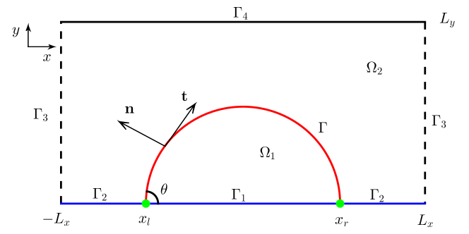
Figure 1: A schematic illustration of the moving contact lines (green points labeled as $x_{l}$ and $x_{r}$) in two-phase flows in a bounded domain $\Omega=\Omega_{1}\cup\Omega_{2}=[-L_{x},~{}L_{x}]\times[0,~{}L_{y}]$, where the red solid line and blue solid line represent the fluid interface $\Gamma$ and the rigid solid substrate $\Gamma_{1}\cup\Gamma_{2}$, respectively.

Without loss of generality, we consider the dynamics of a liquid droplet on a stationary solid substrate in the 2d space, as shown in Fig. 1. We use Cartesian coordinates, where the substrate is on the $x$ axis. The physical domain $\Omega$ consists of two regions: one is occupied by the droplet and denoted by $\Omega_{1}$, the other is occupied by the fluid outside the droplet and denoted by $\Omega_{2}$.

Let $\rho_{i}\ (i=1,2)$ denote the density of the fluids, $\mathbf{u}(\mathbf{x},~{}t):\;\Omega\times[0,T]\rightarrow\mathbb{R}^{2}$ be the fluid velocity, and $p(\mathbf{x},~{}t):\;\Omega\times[0,T]\rightarrow\mathbb{R}$ be the pressure. The dynamics of the system is governed by the standard incompressible Navier-Stokes equations in $\Omega_{i}$ ($i=1,2$),

$$\rho_{i}\,(\partial_{t}\mathbf{u}+\mathbf{u}\cdot\nabla\mathbf{u})=-\nabla p+\nabla\cdot\tau_{d},$$ (2.1a)

$$\nabla\cdot\mathbf{u}=0,$$ (2.1b)

where $\tau_{d}=2\eta_{i}D(\mathbf{u})$ is the viscous stress with $D(\mathbf{u})=\frac{1}{2}(\nabla\mathbf{u}+(\nabla\mathbf{u})^{T})$, and $\eta_{i}\ (i=1,2)$ are the viscosities of the fluids.

On the fluid interface $\Gamma(t)$, we have the following conditions hold

$$\bigl{[}\mathbf{u}\bigr{]}^{2}_{1}=0,$$ (2.2a)

$$\bigl{[}p\mathbf{I}-\tau_{d}\bigr{]}_{1}^{2}\cdot\mathbf{n}=\gamma\kappa\mathbf{n},$$ (2.2b)

$$\dot{\mathbf{x}}_{\Gamma}=\mathbf{u}|_{\mathbf{x}_{\Gamma}},$$ (2.2c)

where $\bigl{[}\cdot\bigr{]}_{1}^{2}$ denotes the jump from fluid 1 to fluid 2, $\mathbf{I}\in\mathbb{R}^{2\times 2}$ is the identity matrix, $\gamma$ is the surface tension of the fluid interface, $\mathbf{n}$ and $\kappa$ are the unit normal vector and curvature of the fluid interface $\Gamma$ respectively, and $\dot{\mathbf{x}}_{\Gamma}$ denotes the velocity of the fluid interface. Eq. (2.2a) states that the fluid velocity is continuous across the interface, Eq. (2.2b) is the balance of the normal stress jump of the fluids and the capillary force, and Eq. (2.2c) is the kinematic condition for the interface.

At the lower solid wall $\Gamma_{1}\cup\Gamma_{2}$, the fluid velocity satisfies the no-penetration condition and the Navier boundary condition

$$\mathbf{u}\cdot\mathbf{n}_{w}=0,$$ (2.3a)

$$\mathbf{t}_{w}\cdot\tau_{d}\cdot\mathbf{n}_{w}=-\beta_{i}u_{s},$$ (2.3b)

where $\mathbf{n}_{w}=(0,-1)^{T}$ and $\mathbf{t}_{w}=(1,0)^{T}$ are unit normal and tangent vectors of the wall, respectively; $\beta_{i}\ (i=1,2)$ are the friction coefficients of the fluids at the solid wall, and $u_{s}=\mathbf{u}\cdot\mathbf{t}_{w}$ is the slip velocity of the fluids. The dynamic contact angles $\theta_{d}^{l}$ and $\theta_{d}^{r}$ that the fluid interface forms with the solid wall satisfy

$$\gamma\left(\cos(\theta_{d}^{l})-\cos\theta_{Y}\right)=\beta^{*}\dot{x}_{l},$$ (2.4a)

$$\gamma\left(\cos(\theta_{d}^{r})-\cos\theta_{Y}\right)=-\beta^{*}\dot{x}_{r},$$ (2.4b)

where $\beta^{*}$ is the friction coefficient of the fluid interface at the solid wall, $\dot{x}_{l}$ and $\dot{x}_{r}$ are the velocities of the contact points, and $\theta_{Y}$ is the equilibrium contact angle satisfying the Young’s relation

$$\gamma\cos\theta_{Y}=\gamma_{2}-\gamma_{1},$$ (2.5)

where $\gamma_{1}$ and $\gamma_{2}$ are the surface tension coefficient at the interface $\Gamma_{1}$ and $\Gamma_{2}$, respectively. We note that since the fluid interface evolves with the fluid velocity according to Eq. (2.2c), we have $\dot{x}_{l,r}=u_{s}\big{|}_{x=x_{l,r}}$. Finally, we use the no-slip condition at the upper wall $\Gamma_{4}$ and periodic conditions at $\Gamma_{3}$.

The total energy of the system is given by

$$E(t)=\sum_{i=1,2}\int_{\Omega_{i}(t)}\frac{1}{2}\rho_{i}|\mathbf{u}|^{2}\;d\mathcal{L}^{2}+(\gamma_{1}-\gamma_{2})|\Gamma_{1}(t)|+\gamma|\Gamma(t)|,$$ (2.6)

where $|\Gamma_{1}(t)|$ and $|\Gamma(t)|$ denote the arc length of the line segment $\Gamma_{1}(t)$ and the curve $\Gamma(t)$, respectively. The three terms represent the kinetic energy of the fluids, the interracial energy at the solid wall and the interfacial energy of the fluid interface, respectively. The dynamical system obeys the following energy dissipation law [5, 36, 20]:

$$\frac{{\rm d}}{{\rm d}t}E(t)=-\sum_{i=1,2}\int_{\Omega_{i}}\eta_{i}|\nabla\mathbf{u}|^{2}\;d\mathcal{L}^{2}-\sum_{i=1,2}\int_{\Gamma_{i}}\beta_{i}|u_{s}|^{2}\;ds-\beta^{*}\left(\dot{x}_{l}^{2}+\dot{x}_{r}^{2}\right)\leq 0.$$ (2.7)

2.2 Dimensionless equations

Next, we write the governing equations and boundary/interface conditions in their dimensionless form. We rescale the physical quantities as

$$\hat{\rho}_{i}=\frac{\rho_{i}}{\rho_{2}},\quad\hat{\eta_{i}}=\frac{\eta_{i}}{\eta_{2}},\quad\hat{\beta_{i}}=\frac{\beta_{i}}{\beta_{2}},\quad\hat{\beta^{*}}=\frac{\beta^{*}}{\eta_{2}},\quad\hat{\gamma}_{i}=\frac{\gamma_{i}}{\gamma},$$

$$\hat{\mathbf{x}}=\frac{\mathbf{x}}{L},\quad\hat{\mathbf{u}}=\frac{\mathbf{u}}{U},\quad\hat{t}=\frac{Ut}{L},\quad\hat{p}=\frac{p}{\rho_{2}U^{2}},\quad\hat{\kappa}=L\kappa,$$

where $L$ and $U$ are the characteristic length and velocity, respectively. We define the Reynolds number $Re$, the Capillary number $Ca$, the slip length $l_{s}$, and the Weber number $We$ as follows,

$$Re=\frac{\rho_{2}UL}{\eta_{2}},\quad Ca=\frac{\eta_{2}U}{\gamma},\quad l_{s}=\frac{\eta_{2}}{\beta_{2}L},\quad We=Re\cdot Ca.$$

Then the governing equations in $\Omega_{i}\ (i=1,2)$ can be rewritten as (dropping the hats):

$$\rho_{i}\,(\partial_{t}\mathbf{u}+\mathbf{u}\cdot\nabla\mathbf{u})+\nabla\cdot\sigma=0,$$ (2.8a)

$$\nabla\cdot\mathbf{u}=0,$$ (2.8b)

where $\sigma=p\mathbf{I}-\frac{1}{Re}\tau_{d}$. The above governing equations are coupled with the following boundary/interface conditions:

• The interface conditions on $\Gamma(t)$:

  $$\bigl{[}\mathbf{u}\bigr{]}^{2}_{1}=0,$$ (2.9a)

  $$We\,\bigl{[}\sigma\bigr{]}_{1}^{2}\cdot\mathbf{n}=\kappa\,\mathbf{n},$$ (2.9b)

  $$\kappa=(\partial_{ss}\mathbf{X})\cdot\mathbf{n},$$ (2.9c)

  $$\dot{\mathbf{x}}_{\Gamma}=\mathbf{u}|_{\mathbf{x}_{\Gamma}}.$$ (2.9d)

  where $s$ is the arc-length parameter of the fluid interface.

• The boundary conditions on $\Gamma_{1}(t)\cup\Gamma_{2}(t)$:

  $$\mathbf{u}\cdot\mathbf{n}_{w}=0,$$ (2.10a)

  $$l_{s}\,\mathbf{t}_{w}\cdot\tau_{d}\cdot\mathbf{n}_{w}=-\beta_{i}u_{s}.$$ (2.10b)

• The condition for the dynamic contact angles:

  $$\frac{1}{Ca}(\cos\theta_{d}^{l}-\cos\theta_{Y})=\beta^{*}\dot{x}_{l}(t),$$ (2.11a)

  $$\frac{1}{Ca}(\cos\theta_{d}^{r}-\cos\theta_{Y})=-\beta^{*}\dot{x}_{r}(t).$$ (2.11b)

• Periodic boundary conditions on $\Gamma_{3}$:

  $$\mathbf{u}(-L_{x},y,t)=\mathbf{u}(L_{x},y,t),$$ (2.12a)

  $$\sigma(-L_{x},y,t)=\sigma(L_{x},y,t).$$ (2.12b)

• The no-slip condition on the upper wall $\Gamma_{4}$:

  $$\mathbf{u}=\mathbf{0}.$$ (2.13)

In terms of the dimensionless variables, the total energy (rescaled by $\rho_{2}U^{2}L^{2}$) of the system becomes

$$E(t)=\sum_{i=1,2}\int_{\Omega_{i}(t)}\frac{1}{2}\rho_{i}|\mathbf{u}|^{2}\;d\mathcal{L}^{2}-\frac{\cos\theta_{Y}}{We}|\Gamma_{1}(t)|+\frac{1}{We}|\Gamma(t)|,$$ (2.14)

and the system obeys the energy dissipation law

$$\frac{{\rm d}}{{\rm d}t}E(t)=-\sum_{i=1,2}\frac{1}{Re}\int_{\Omega_{i}}\eta_{i}|\nabla\mathbf{u}|^{2}\;d\mathcal{L}^{2}-\sum_{i=1,2}\frac{1}{Re\,l_{s}}\int_{\Gamma_{i}}\beta_{i}|u_{s}|^{2}\;ds-\frac{\beta^{*}}{Re}\left(\dot{x}_{l}^{2}+\dot{x}_{r}^{2}\right)\leq 0.$$ (2.15)

2.3 Weak formulation

In order to propose the weak formulation for equations (2.8) - (2.13), we define the following function space for the fluid velocity,

$$\mathbb{U}:=\left\{\boldsymbol{\omega}\in\left[H^{1}(\Omega)\right]^{2}:\;\boldsymbol{\omega}\cdot\mathbf{n}_{w}=0\;{\rm on}\;\Gamma_{1}\cup\Gamma_{2},\;\boldsymbol{\omega}=\mathbf{0}\;{\rm on}\;\Gamma_{4},\;{\rm and}\;\boldsymbol{\omega}(-L_{x},~{}y)=\boldsymbol{\omega}(L_{x},~{}y)\right\},$$ (2.16)

and the following function spaces for the pressure,

$$\mathbb{P}:=\left\{\varphi\in L^{2}(\Omega)\right\},\qquad\hat{\mathbb{P}}:=\left\{\varphi\in\mathbb{P}:\;\int_{\Omega}\varphi d\mathcal{L}^{2}=0\right\}.$$ (2.17)

We parameterize the fluid interface as $\mathbf{X}(\alpha,t)=(X(\alpha,t),Y(\alpha,t))$, where $\alpha\in I=[0,1]$, and $\alpha=0,\ 1$ correspond to the left and right contact point, respectively. We define the following function space with respect to the interface,

$$L^{2}(I)=\left\{u:I\rightarrow\mathbb{R},\;\text{and}\int_{I}|u(\alpha)|^{2}|\partial_{\alpha}\mathbf{X}|\,d\alpha<+\infty\right\},$$ (2.18)

equipped with the inner product

$$\big{(}u,v\big{)}_{\Gamma}=\int_{I}u(\alpha)v(\alpha)|\partial_{\alpha}\mathbf{X}|\,d\alpha,\quad\forall\;u,v\in L^{2}(I).$$ (2.19)

We take the inner product of Eq. (2.8a) with $\boldsymbol{\omega}$, for $\forall\boldsymbol{\omega}\in\mathbb{U}$. Using the boundary/interface conditions in (2.9), (2.10), (2.12) and (2.13), as well as $\nabla\cdot\mathbf{u}=0$, we have [50, 51]

$$\Bigl{(}\rho\,[\partial_{t}\mathbf{u}+(\mathbf{u}\cdot\nabla)\mathbf{u}],\boldsymbol{\omega}\Bigr{)}=\frac{1}{2}\,\left[\frac{\rm{d}}{\rm{d}t}\Bigl{(}\rho\,\mathbf{u},\boldsymbol{\omega}\Bigr{)}+\Bigl{(}\rho\,\partial_{t}\mathbf{u},\boldsymbol{\omega}\Bigr{)}\right]+\frac{1}{2}\,\Bigl{(}\rho,[(\mathbf{u}\cdot\nabla)\mathbf{u}]\cdot\boldsymbol{\omega}-[(\mathbf{u}\cdot\nabla)\boldsymbol{\omega}]\cdot\mathbf{u}\Bigl{)},$$ (2.20)

where $\rho=\rho_{1}\chi_{{}_{\Omega_{1}}}+\rho_{2}\chi_{{}_{\Omega_{2}}}$, $\chi$ is the characteristic function, and $(\cdot,\cdot)$ denotes the $L^{2}$ inner product on $\Omega_{1}\cup\Omega_{2}$,

$$(\mathbf{u},\mathbf{v})=\sum_{i=1,2}\int_{\Omega_{i}}\mathbf{u}\cdot\mathbf{v}d\mathcal{L}^{2}.$$

For the viscous term, take the inner product with $\boldsymbol{\omega}\in\mathbb{U}$. We use $\sigma=p\mathbf{I}-\frac{1}{Re}\tau_{d}$, and apply integration by parts, which yields

$$\Bigl{(}\nabla\cdot\sigma,\boldsymbol{\omega}\Bigr{)} =-\Bigl{(}p,~{}\nabla\cdot\boldsymbol{\omega}\Bigr{)}+\frac{2}{Re}\Bigl{(}\eta D(\mathbf{u}),~{}D(\boldsymbol{\omega})\Bigr{)}-\Bigl{(}[\sigma]_{1}^{2}\cdot\mathbf{n},~{}\boldsymbol{\omega}\Bigr{)}_{\Gamma}+\Bigl{(}\sigma\cdot\mathbf{n}_{w},~{}\boldsymbol{\omega}\Bigr{)}_{\Gamma_{1}\cup\Gamma_{2}}$$

$$=-\Bigl{(}p,~{}\nabla\cdot\boldsymbol{\omega}\Bigr{)}+\frac{2}{Re}\Bigl{(}\eta D(\mathbf{u}),D(\boldsymbol{\omega})\Bigr{)}-\frac{1}{We}\Bigl{(}\kappa\,\mathbf{n},\boldsymbol{\omega}\Bigr{)}_{\Gamma}-\frac{1}{Re}\Bigl{(}\tau_{d}\cdot\mathbf{n}_{w},\boldsymbol{\omega}\Bigr{)}_{\Gamma_{1}\cup\Gamma_{2}}$$

$$=-\Bigl{(}p,\nabla\cdot\boldsymbol{\omega}\Bigr{)}+\frac{2}{Re}\Bigl{(}\eta D(\mathbf{u}),D(\boldsymbol{\omega})\Bigr{)}-\frac{1}{We}\Bigl{(}\kappa\,\mathbf{n},\boldsymbol{\omega}\Bigr{)}_{\Gamma}+\frac{1}{Re\,l_{s}}\Bigl{(}\beta\,u_{s},\omega_{s})_{\Gamma_{1}\cup\Gamma_{2}},$$ (2.21)

where $\eta=\eta_{1}\chi_{{}_{\Omega_{1}}}+\eta_{2}\chi_{{}_{\Omega_{2}}}$, $\beta=\beta_{1}\chi_{{}_{\Gamma_{1}}}+\beta_{2}\chi_{{}_{\Gamma_{2}}}$, $\omega_{s}=\boldsymbol{\omega}\cdot\mathbf{t}_{w}$, and we have used the boundary and interface conditions and the fact that $\boldsymbol{\omega}=(\boldsymbol{\omega}\cdot\mathbf{t}_{w})\,\mathbf{t}_{w}=\omega_{s}\,\mathbf{t}_{w}$ on $\Gamma_{1}\cup\Gamma_{2}$.

Equation (2.9c) for the curvature can be rewritten as $\kappa\,\mathbf{n}=\partial_{ss}\mathbf{X}$. Multiplying this equation by a test function $\mathbf{g}=(g_{1},g_{2})\in H^{1}(I)\times H_{0}^{1}(I)$ then integrating over $\Gamma(t)$ yields

$$0 =\Bigl{(}\kappa,\mathbf{n}\cdot\mathbf{g}\Bigr{)}_{\Gamma}+\Bigl{(}\partial_{s}\mathbf{X},\partial_{s}\mathbf{g}\Bigr{)}_{\Gamma}-(\partial_{s}\mathbf{X}\cdot\mathbf{g})\Big{|}_{\alpha=0}^{\alpha=1}$$

$$=\Bigl{(}\kappa,\mathbf{n}\cdot\mathbf{g}\Bigr{)}_{\Gamma}+\Bigl{(}\partial_{s}\mathbf{X},\partial_{s}\mathbf{g}\Bigr{)}_{\Gamma}-(g_{1}\partial_{s}X)\Big{|}_{\alpha=0}^{\alpha=1}$$

$$=\Bigl{(}\kappa,\mathbf{n}\cdot\mathbf{g}\Bigr{)}_{\Gamma}+\Bigl{(}\partial_{s}\mathbf{X},\partial_{s}\mathbf{g}\Bigr{)}_{\Gamma}+\beta^{*}\,Ca\left[\dot{x}_{l}g_{1}(0)+\dot{x}_{r}g_{1}(1)\right]-\cos\theta_{Y}\left[g_{1}(1)-g_{1}(0)\right],$$ (2.22)

where we have used fact that $g_{2}(0)=g_{2}(1)=0$ in the second equality, and $\partial_{s}X|_{\alpha=0}=\cos\theta_{d}^{l},\,\partial_{s}X|_{\alpha=1}=\cos\theta_{d}^{r}$ and the contact angle condition (2.11) in the last equality.

From these results, we obtain the weak formulation for the dynamic system Eqs. (2.8)-(2.13) as follows: Given the initial fluid velocity $\mathbf{u}_{0}$ and interface $\mathbf{X}_{0}(\alpha)$, find the fluid velocity $\mathbf{u}(\cdot,~{}t)\in\mathbb{U}$, the pressure $p(\cdot,~{}t)\in\hat{\mathbb{P}}$, the fluid interface $\Gamma(t):=\mathbf{X}(\cdot,~{}t)\in\ H^{1}(I)\times H_{0}^{1}(I)$, and the curvature $\kappa(\cdot,~{}t)\in L^{2}(I)$ such that

$$\frac{1}{2}\,\Bigl{[}\frac{{\rm d}}{{\rm d}t}\Bigl{(}\rho\,\mathbf{u},~{}\boldsymbol{\omega}\Bigr{)}+\Bigl{(}\rho\,\partial_{t}\mathbf{u},~{}\boldsymbol{\omega}\Bigr{)}+\Bigl{(}\rho\,(\mathbf{u}\cdot\nabla)\mathbf{u},~{}\boldsymbol{\omega}\Bigr{)}-\Bigl{(}\rho\,(\mathbf{u}\cdot\nabla)\boldsymbol{\omega},~{}\mathbf{u}\Bigr{)}\Bigr{]}+\frac{2}{Re}\,\Bigl{(}\eta D(\mathbf{u}),~{}D(\boldsymbol{\omega})\Bigr{)}$$

$$\qquad\qquad-\Bigl{(}p,~{}\nabla\cdot\boldsymbol{\omega}\Bigr{)}-\frac{1}{We}\Bigl{(}\kappa\,\mathbf{n},~{}\boldsymbol{\omega}\Bigr{)}_{\Gamma}+\,\frac{1}{Re\,l_{s}}\Bigl{(}\beta\,u_{s},~{}\omega_{s}\Bigr{)}_{\Gamma_{1}\cup\Gamma_{2}}=0,\qquad\forall\boldsymbol{\omega}\in\mathbb{U},$$ (2.23a)

$$\qquad\qquad\qquad\qquad\qquad\qquad\qquad\Bigl{(}\nabla\cdot\mathbf{u},~{}q\Bigr{)}=0,\qquad\forall q\in\hat{\mathbb{P}},$$ (2.23b)

$$\qquad\qquad\qquad\Bigl{(}\partial_{t}\mathbf{X}\cdot\mathbf{n},~{}\psi\Bigr{)}_{\Gamma}-\Bigl{(}\mathbf{u}\cdot\mathbf{n},~{}\psi\Bigr{)}_{\Gamma}=0,\qquad\forall\psi\in L^{2}(I),$$ (2.23c)

$$\Bigl{(}\kappa\,\mathbf{n},~{}\boldsymbol{g}\Bigr{)}_{\Gamma}+\Bigl{(}\partial_{s}\mathbf{X},~{}\partial_{s}\boldsymbol{g}\Bigr{)}_{\Gamma}+\beta^{*}Ca\Bigl{[}\dot{x}_{l}g_{1}(0)+\dot{x}_{r}g_{1}(1)\Bigr{]}-\cos\theta_{Y}[g_{1}(1)-g_{1}(0)]=0,$$

$$\qquad\qquad\qquad\qquad\hskip 199.16928pt\forall\boldsymbol{g}\in H^{1}(I)\times H_{0}^{1}(I).$$ (2.23d)

Eq. (2.23) is a direct result from Eq. (2.20) and Eq. (2.21). Eq. (2.23b) is from the incompressibility condition. Eq. (2.23c) is obtained from the kinematic condition (2.9d), after rewriting it as $\partial_{t}\mathbf{X}\cdot\mathbf{n}=\mathbf{u}\cdot\mathbf{n}$ with $Y(0)=Y(1)=0$. Eq. (2.23) is obtained from Eq. (2.22).

The system (2.23) - (2.23) is an extension of the weak formulation introduced in Ref. [50] for two-phase flows. Here we have extended it two-phase flows with moving contact lines. One can prove the energy dissipation and mass/area conservation properties within the weak formulation in a similar manner as did in Ref. [50].

3 The numerical method

Next, we present a finite element method (FEM) based on the weak formulation (2.23)-(2.23) and show the well-posedness and stability for the discretized system. Moreover, we propose a moving mesh approach for the construction of the mesh such that the fluid interface remains fitted to the mesh at each time step.

3.1 The finite element method

We partition the time domain $[0,T]$ as $0=t_{0}<t_{1}<t_{2}<\cdots<t_{M}=T$ with the time steps $\tau_{m}=t_{m+1}-t_{m}\;(m=0,\cdots,M-1)$ and the reference domain $I=[0,1]$ for the fluid interface as $I=\bigcup_{j=1}^{J_{{}_{\Gamma}}}I_{j}$, where $I_{j}=[\alpha_{j-1},\alpha_{j}]$ with $\alpha_{j}=jh$ and $h=1/J_{{}_{\Gamma}}$. We use the following finite-dimensional spaces to approximate $H^{1}(I)$ and $H^{1}_{0}(I)$, respectively,

$$V^{h}: =\left\{u\in C(I):\;u\mid_{I_{j}}\in\mathcal{P}_{1}(I_{j}),\quad\forall\,j=1,2,\ldots,J_{{}_{\Gamma}}\right\}$$ (3.1a)

$$V_{0}^{h}: =\left\{u\in V^{h}:u(0)=u(1)=0\right\},$$ (3.1b)

where $\mathcal{P}_{1}$ denotes the space of polynomials with degrees at most 1.

Let $\Gamma^{m}:=\mathbf{X}^{m}(\cdot)\in V^{h}\times V_{0}^{h}$ be the numerical approximation to the fluid interface $\Gamma$ at the time $t=t_{m}$. For piecewise continuous functions $u$ and $v$ defined on the interval $I$ with possible jumps at the nodes $\{\alpha_{j}\}_{j=1}^{J_{{}_{\Gamma}}-1}$, we approximate the inner product $(u,v)_{\Gamma(t_{m})}$ by either the Simpson rule $\big{(}u,~{}v\big{)}_{\Gamma^{m}}$ or the Trapezoidal rule $\big{(}u,v\big{)}_{\Gamma^{m}}^{h}$ (the mass-lumped norm) as

$$\big{(}u,v\big{)}_{\Gamma^{m}}:=\frac{1}{6}\sum_{j=1}^{J_{\Gamma}}\Big{|}\mathbf{X}^{m}(\alpha_{j})-\mathbf{X}^{m}(\alpha_{j-1})\Big{|}\Big{[}\big{(}u\cdot v\big{)}(\alpha_{j-1}^{+})+4\big{(}u\cdot v\big{)}(\alpha_{j-\frac{1}{2}})+\big{(}u\cdot v\big{)}(\alpha_{j}^{-})\Big{]},$$ (3.2)

$$\big{(}u,v\big{)}_{\Gamma^{m}}^{h}:=\frac{1}{2}\sum_{j=1}^{J_{\Gamma}}\Big{|}\mathbf{X}^{m}(\alpha_{j})-\mathbf{X}^{m}(\alpha_{j-1})\Big{|}\Big{[}\big{(}u\cdot v\big{)}(\alpha_{j-1}^{+})+\big{(}u\cdot v\big{)}(\alpha_{j}^{-})\Big{]},$$ (3.3)

where $u(\alpha_{j}^{\pm})$ are the one-sided limits of $u$ at $\alpha_{j}$ and $\alpha_{j-\frac{1}{2}}=\frac{1}{2}(\alpha_{j-1}+\alpha_{j})$. Let $\mathbf{n}^{m}$ and $\kappa^{m}$ be the numerical approximations to the normal vector and the curvature of $\Gamma(t_{m})$, respectively. On each interval $I_{j}$, the normal vector $\mathbf{n}^{m}$ is a constant vector and is computed as

$$\mathbf{n}_{j}^{m}:=\mathbf{n}^{m}\Big{|}_{I_{j}}=[\partial_{s}\mathbf{X}^{m}]^{\perp}\Big{|}_{I_{j}}=\frac{\left[\mathbf{X}^{m}(\alpha_{j})-\mathbf{X}^{m}(\alpha_{j-1})\right]^{\perp}}{\left|\mathbf{X}^{m}(\alpha_{j})-\mathbf{X}^{m}(\alpha_{j-1})\right|},\quad 1\leq j\leq J_{{}_{\Gamma}},$$ (3.4)

where $(\cdot)^{\perp}$ denotes the counterclockwise rotation by $\frac{\pi}{2}$. In the following, we shall assume $\forall 0\leq m\leq M$,

$$\Gamma^{m}\;\text{has no self-intersections},$$ (3.5a)

$$n^{m,1}_{1}\neq 0,\quad n^{m,1}_{J_{{}_{\Gamma}}}\neq 0,$$ (3.5b)

$$\left|\partial_{\alpha}\mathbf{X}^{m}\right|>0,$$ (3.5c)

where $\mathbf{n}^{m}_{j}=\bigl{(}n_{j}^{m,1},n_{j}^{m,2}\bigr{)}$. These conditions imply that (1) the first and last line segments of $\Gamma^{m}$ are not parallel to the $x$-axis; (2) the mesh points on $\{\Gamma^{m}\}_{m=1}^{M}$ do not merge.

Let $\mathcal{T}^{m}:=\bigcup_{j=1}^{N}\bar{o}_{j}^{m}$ be a triangulation of $\Omega$ at the time step $t=t_{m}$. The mesh contains $J_{\Omega}$ vertices denoted by $\left\{\mathbf{q}_{k}^{m}\right\}_{k=1}^{J_{\Omega}}$. We use a fitted mesh such that the interface $\Gamma^{m}$ is fitted to the triangular mesh $\mathcal{T}^{m}$. Specifically, the line segments of $\Gamma^{m}$ are edges of triangles from the mesh, i.e., $\Gamma^{m}\subset\bigcup_{j=1}^{N}\partial o_{j}^{m}$. We define the following finite element spaces over $\mathcal{T}^{m}$,

$$S_{k}^{m}: =\left\{\varphi_{h}\in C(\bar{\Omega}):\varphi_{h}|_{o_{j}^{m}}\in\mathcal{P}_{k}(o_{j}^{m}),\;j=1,\cdots,N\right\},$$ (3.6a)

$$S_{0}^{m}: =\{\varphi_{h}\in L^{2}(\Omega):\varphi_{h}|_{o_{j}^{m}}\in\mathcal{P}_{0}(o_{j}^{m}),\;j=1,\cdots,N\},$$ (3.6b)

where $k\in\mathbb{N}^{+}$, and $\mathcal{P}_{k}(o_{j}^{m})$ denotes the space of polynomials of degree k on $o_{j}^{m}$.

The interface $\Gamma^{m}$ divides the domain $\Omega$ into $\Omega_{1}^{m}$ and $\Omega_{2}^{m}$. Correspondingly, the mesh $\mathcal{T}^{m}$ is divided into $\mathcal{T}_{1}^{m}$ and $\mathcal{T}_{2}^{m}$, which consist of triangles in $\Omega_{1}^{m}$ and $\Omega_{2}^{m}$, respectively. Based on the spatial discetization, we define the friction coefficient $\beta^{m}$ and the viscosity $\eta^{m}\in S_{0}^{m}$ as

$$\beta^{m}=\beta_{1}\chi_{{}_{\Gamma_{1}^{m}}}+\beta_{2}\chi_{{}_{\Gamma_{2}^{m}}},\quad\eta^{m}=\eta_{1}\chi_{{}_{\Omega_{1}^{m}}}+\eta_{2}\chi_{{}_{\Omega_{2}^{m}}}.$$ (3.7)

Moreover, we define the density $\rho^{m}\in S_{1}^{m}$ such that at the vertices $\{\mathbf{q}_{k}^{m}\}_{k=1}^{J_{\Omega}}$ it takes the value

$$\left.\rho^{m}\right|_{\mathbf{x}=\mathbf{q}_{k}^{m}}=\left\{\begin{array}[]{ll}\rho_{1},&\mbox{if}\ \mathbf{q}_{k}^{m}\in\bar{\Omega}_{1}^{m}\backslash\Gamma^{m},\vspace{0.15cm}\\ \frac{1}{2}(\rho_{1}+\rho_{2}),&\mbox{if}\ \mathbf{q}_{k}^{m}\in\Gamma^{m},\vspace{0.15cm}\\ \rho_{2},&\mbox{if}\ \mathbf{q}_{k}^{m}\in\bar{\Omega}_{2}^{m}\backslash\Gamma^{m}.\end{array}\right.$$ (3.8)

We note that the density $\rho^{m}$ is a continuous function instead of a piecewise constant function. This facilitates the interpolation of $\rho^{m}$ from the mesh $\mathcal{T}^{m}$ to the mesh $\mathcal{T}^{m+1}$ which is required in the numerical method.

Let $\mathbb{U}^{m}$ and $\hat{\mathbb{P}}^{m}$ denote the finite element spaces for the numerical solution for the velocity and pressure, respectively. We use the following two pairs of elements for $\left(\mathbb{U}^{m},~{}\hat{\mathbb{P}}^{m}\right)$,

$${\rm P2-P0}:\ \left(\mathbb{U}^{m},~{}\hat{\mathbb{P}}^{m}\right)=\left([S_{2}^{m}]^{2}\cap\mathbb{U},~{}S_{0}^{m}\cap\hat{\mathbb{P}}\right),$$ (3.9a)

$${\rm P2-(P1+P0)}:\ \left(\mathbb{U}^{m},~{}\hat{\mathbb{P}}^{m}\right)=\left([S_{2}^{m}]^{2}\cap\mathbb{U},~{}(S_{1}^{m}+S_{0}^{m})\cap\hat{\mathbb{P}}\right),$$ (3.9b)

where $\mathbb{U}$ and $\hat{\mathbb{P}}$ are defined in (2.16) and (2.17), respectively. These two choices satisfy the inf-sup stability condition [50, 52],

$$\inf_{\varphi\in\hat{\mathbb{P}}^{m}}\sup_{\mathbf{0}\neq\boldsymbol{\omega}\in\mathbb{U}^{m}}\frac{\left(\varphi,\nabla\cdot\boldsymbol{\omega}\right)}{\lVert\varphi\rVert_{0}\lVert\boldsymbol{\omega}\rVert_{1}}\geq C_{0}>0,$$ (3.10)

where $\lVert\cdot\rVert_{0}$ and $\lVert\cdot\rVert_{1}$ denote the $L^{2}$ and $H^{1}$-norm on $\Omega$ respectively, and $C_{0}$ is a constant. The finite element spaces for the pressure can catch the discontinuity of the pressure across the fluid interface.

We use $V^{h}\times V_{0}^{h}$ and $V^{h}$ as the finite element space for the fluid interface and its curvature, respectively. The finite element method is given as follows. Let $\Gamma^{0}:=\mathbf{X}^{0}(\cdot)\in V^{h}\times V_{0}^{h}$ and $\mathcal{T}^{0}$ be the discretization of the initial interface $\Gamma(0)$ and the triangulation of the domain $\Omega(0)$, respectively, and $\mathbf{u}^{0}=I_{2}^{0}\mathbf{u}_{0}\in\mathbb{U}^{0}$ be the discretization of the initial fluid velocity $\mathbf{u}_{0}$. For $m\geq 0$, find $\mathbf{u}^{m+1}\in\mathbb{U}^{m}$, $p^{m+1}\in\hat{\mathbb{P}}^{m}$, $\mathbf{X}^{m+1}\in V^{h}\times V_{0}^{h}$, and $\kappa^{m+1}\in V^{h}$ by solving the linear system

$$\frac{1}{2}\Bigl{[}\Bigl{(}\frac{\rho^{m}\mathbf{u}^{m+1}-(I_{1}^{m}\rho^{m-1})I_{2}^{m}\mathbf{u}^{m}}{\tau_{m}},~{}\boldsymbol{\omega}^{h}\Bigr{)}+\Bigl{(}I_{1}^{m}\rho^{m-1}\frac{\mathbf{u}^{m+1}-I_{2}^{m}\mathbf{u}^{m}}{\tau_{m}},~{}\boldsymbol{\omega}^{h}\Bigr{)}+\Bigl{(}\rho^{m}(I_{2}^{m}\mathbf{u}^{m}\cdot\nabla)\mathbf{u}^{m+1},~{}\boldsymbol{\omega}^{h}\Bigr{)}$$

$$\qquad\qquad-\Bigl{(}\rho^{m}(I_{2}^{m}\mathbf{u}^{m}\cdot\nabla)\boldsymbol{\omega}^{h},~{}\mathbf{u}^{m+1}\Bigr{)}\Bigr{]}-\Bigl{(}p^{m+1},~{}\nabla\cdot\boldsymbol{\omega}^{h}\Bigr{)}+\frac{2}{Re}\Bigl{(}\eta^{m}D(\mathbf{u}^{m+1}),~{}D(\boldsymbol{\omega}^{h})\Bigr{)}$$

$$\qquad\qquad-\frac{1}{We}\Bigl{(}\kappa^{m+1}\mathbf{n}^{m},~{}\boldsymbol{\omega}^{h}\Bigr{)}_{\Gamma^{m}}+\frac{1}{Re\cdot l_{s}}\Bigr{(}\beta^{m}\,u_{s}^{m+1},~{}\omega_{s}^{h}\Bigr{)}_{\Gamma_{1}^{m}\cup\Gamma_{2}^{m}}=0,\quad\forall\boldsymbol{\omega}^{h}\in\mathbb{U}^{m},$$ (3.11a)

$$\qquad\qquad\qquad\qquad\qquad\Bigl{(}\nabla\cdot\mathbf{u}^{m+1},~{}q^{h}\Bigr{)}=0,\qquad\forall q^{h}\in\hat{\mathbb{P}}^{m},$$ (3.11b)

$$\qquad\qquad\Bigl{(}\frac{\mathbf{X}^{m+1}-\mathbf{X}^{m}}{\tau_{m}}\cdot\mathbf{n}^{m},~{}\psi^{h}\Bigr{)}_{\Gamma^{m}}^{h}-\Bigl{(}\mathbf{u}^{m+1}\cdot\mathbf{n}^{m},~{}\psi^{h}\Bigr{)}_{\Gamma^{m}}=0,\quad\forall\psi^{h}\in V^{h},$$ (3.11c)

$$\Bigl{(}\kappa^{m+1}\,\mathbf{n}^{m},~{}\boldsymbol{g}^{h}\Bigr{)}_{\Gamma^{m}}^{h}+\Bigl{(}\partial_{s}\mathbf{X}^{m+1},~{}\partial_{s}\boldsymbol{g}^{h}\Bigr{)}_{\Gamma^{m}}-\cos\theta_{Y}\left[g_{1}^{h}(1)-g_{1}^{h}(0)\right]$$

$$\qquad\qquad\qquad+\frac{\beta^{*}Ca}{\tau_{m}}\Bigl{[}\left(x^{m+1}_{r}-x^{m}_{r}\right)g_{1}^{h}(1)+\left(x^{m+1}_{l}-x_{l}^{m}\right)g_{1}^{h}(0)\Bigr{]}=0,\quad\forall\boldsymbol{g}^{h}\in V^{h}\times V_{0}^{h},$$ (3.11d)

where $\boldsymbol{g}^{h}=(g^{h}_{1},~{}g^{h}_{2})$, $\omega_{s}^{h}=\boldsymbol{\omega}^{h}\cdot\mathbf{t}_{w}$, $u_{s}^{m+1}=\mathbf{u}^{m+1}\cdot\mathbf{t}_{w}$, and $x_{l}^{m}:=X^{m}|_{\alpha=0}$ and $x_{r}^{m}=X^{m}|_{\alpha=1}$ denote the left and right contact points of $\Gamma^{m}$, respectively. For $f\in V^{h}$, $\partial_{s}f:=\frac{1}{|\partial_{\alpha}\mathbf{X}^{m}|}\partial_{\alpha}f$. At the first step, we set $\rho^{-1}=\rho^{0}$.

In the above scheme, $\mathbf{u}^{m}$ and $\rho^{m-1}$ are both obtained on the mesh $\mathcal{T}^{m-1}$, and then used to compute the solutions $(\mathbf{u}^{m+1},\ p^{m+1},\ \mathbf{X}^{m+1},\ \kappa^{m+1})$ on the new mesh $\mathcal{T}^{m}$. Therefore, we need to perform interpolations to obtain their values on the new mesh. The operators $I_{1}^{m}$ and $I_{2}^{m}$ are for this purpose. They denote the linear and quadratic interpolations from $\mathcal{T}^{m-1}$ to $\mathcal{T}^{m}$, respectively.

The numerical scheme is an extension of the earlier work by Barrett et. al. [50] to systems with the moving contact lines. We note that the special treatment of the inertia term in Eq. (2.20) is to maintain the discrete stability for the fluid kinetic energy. Another remark is on the disretization of the temporal derivative $\frac{d}{dt}\bigl{(}\rho\mathbf{u},~{}\boldsymbol{\omega}\bigr{)}$,

$$\frac{d}{dt}\Bigl{(}\rho\mathbf{u},~{}\boldsymbol{\omega}\Bigr{)}\approx\frac{1}{\tau_{m}}\Big{[}\Bigl{(}\rho^{m}\mathbf{u}^{m+1},~{}\boldsymbol{\omega^{h}}\Bigr{)}-\Bigl{(}(I_{1}^{m}\rho^{m-1})(I_{2}^{m}\mathbf{u}^{m}),~{}\boldsymbol{\omega}^{h}\Bigr{)}\Bigr{]}.$$ (3.12)

The density $\rho^{m+1}$ depends on the mesh $\mathcal{T}^{m+1}$ (see the definition in Eq. (3.8)), thus is unknown before the interface $\Gamma^{m+1}$ is computed. Therefore, in the above discretization we avoided using $\rho^{m+1}$ by lagging the density by one time step. This yields a linear system for the solutions at $t=t_{m+1}$.

The numerical scheme is a combination of the finite element method for the incompressible Navier-Stokes equations and the parametric finite element method for the interface evolution. The curvature is introduced as a new variable and treated implicitly in the scheme. This helps to yield the discrete stability for the interfacial energy as discussed next. The different numerical quadratures have been utilized to approximate the inner product over $\Gamma^{m}$, and the approximation by the mass-lumped norm is essential to the property of the equal mesh distribution, which has been discussed in detail in [53].

3.2 Properties of the FEM

Next we show that the numerical method (3.11) - (3.11d) yields a unique solution (Theorem 3.1), and is energy stable (Theorem 3.2).

Theorem 3.1 (Well-posedness).

Let $(\mathbb{U}^{m},~{}\hat{\mathbb{P}}^{m})$ satisfy the inf-sup stability condition (3.10), the interface $\mathbf{X}^{m}(\cdot)$ satisfy the conditions in (3.5). Then the numerical method (3.11)-(3.11d) admits a unique solution.

Proof.

It suffices to show that the corresponding homogeneous system has only zero solution. Thus we consider solving the following homogeneous system for $\big{(}\mathbf{u}^{h},~{}p^{h},~{}\mathbf{X}^{h},~{}\kappa^{h}\big{)}\in\big{(}\mathbb{U}^{m},~{}\hat{\mathbb{P}}^{m},~{}V^{h}\times V_{0}^{h},~{}V^{h}\big{)}$,

$$\frac{1}{2}\Bigl{[}\Bigl{(}\frac{(\rho^{m}+I_{1}^{m}\rho^{m-1})\mathbf{u}^{h}}{\tau_{m}},~{}\boldsymbol{\omega}^{h}\Bigr{)}+\Bigl{(}\rho^{m}(I_{2}^{m}\mathbf{u}^{m}\cdot\nabla)\mathbf{u}^{h},~{}\boldsymbol{\omega}^{h}\Bigr{)}-\Bigl{(}\rho^{m}(I_{2}^{m}\mathbf{u}^{m}\cdot\nabla)\boldsymbol{\omega}^{h},~{}\mathbf{u}^{h}\Bigr{)}\Bigr{]}$$

$$\qquad\qquad-\Bigl{(}p^{h},~{}\nabla\cdot\boldsymbol{\omega}^{h}\Bigr{)}+\frac{2}{Re}\,\Bigl{(}\eta^{m}D(\mathbf{u}^{h}),~{}D(\boldsymbol{\omega}^{h})\Bigr{)}-\frac{1}{We}\Bigl{(}\kappa^{h}\,\mathbf{n}^{m},~{}\boldsymbol{\omega}^{h}\Bigr{)}_{\Gamma^{m}}$$

$$\qquad\qquad\qquad\qquad\hskip 71.13188pt+\frac{1}{Re\cdot l_{s}}\Bigr{(}\beta^{m}\,u_{s}^{h},~{}\omega_{s}^{h}\Bigr{)}_{\Gamma_{1}^{m}\cup\Gamma_{2}^{m}}=0,\quad\forall\boldsymbol{\omega}^{h}\in\mathbb{U}^{m},$$ (3.13a)

$$\qquad\qquad\qquad\qquad\qquad\qquad\Bigl{(}\nabla\cdot\mathbf{u}^{h},~{}q^{h}\Bigr{)}=0,\qquad\forall q^{h}\in\hat{\mathbb{P}}^{m},$$ (3.13b)

$$\qquad\qquad\qquad\Bigl{(}\frac{\mathbf{X}^{h}}{\tau_{m}}\cdot\mathbf{n}^{m},~{}\psi^{h}\Bigr{)}_{\Gamma^{m}}^{h}-\Bigl{(}\mathbf{u}^{h}\cdot\mathbf{n}^{m},~{}\psi^{h}\Bigr{)}_{\Gamma^{m}}=0,\quad\forall\psi^{h}\in V^{h},$$ (3.13c)

$$\Bigl{(}\kappa^{h}\,\mathbf{n}^{m},~{}\boldsymbol{g}^{h}\Bigr{)}_{\Gamma^{m}}^{h}+\Bigl{(}\partial_{s}\mathbf{X}^{h},~{}\partial_{s}\boldsymbol{g}^{h}\Bigr{)}_{\Gamma^{m}}+\frac{\beta^{*}Ca}{\tau_{m}}\Bigl{[}x_{r}^{h}\,g_{1}^{h}(1)+x_{l}^{h}\,g_{1}^{h}(0)\Bigr{]}=0,\quad\forall\boldsymbol{g}^{h}\in V^{h}\times V_{0}^{h},$$ (3.13d)

where $\mathbf{X}^{h}=(X^{h},~{}Y^{h})$, $u_{s}^{h}=\mathbf{u}^{h}\cdot\mathbf{t}_{w}$, and $x_{l}^{h}:=X^{h}|_{\alpha=0}$ and $x_{r}^{h}:=X^{h}|_{\alpha=1}$.

Setting $\boldsymbol{\omega}^{h}=\mathbf{u}^{h}$, $q^{h}=p^{h}$, $\psi^{h}=\frac{1}{We}\kappa^{h}$ and $\boldsymbol{g}^{h}=\frac{1}{We}\mathbf{X}^{h}$, then combinning these equations yields

$$\frac{1}{2}\Bigl{(}(\rho^{m}+I_{1}^{m}\rho^{m-1})\mathbf{u}^{h},~{}\mathbf{u}^{h}\Bigr{)}+\frac{2\tau_{m}}{Re}\Bigl{(}\eta^{m}\,D(\mathbf{u}^{h}),~{}D(\mathbf{u}^{h})\Bigr{)}+\frac{\tau_{m}}{Re\cdot l_{s}}\Bigl{(}\beta^{m}\,u_{s}^{h},~{}u_{s}^{h}\Bigr{)}_{\Gamma_{1}^{m}\cup\Gamma_{2}^{m}}$$

$$\qquad\qquad\hskip 56.9055pt+\frac{1}{We}\Bigl{(}\partial_{s}\mathbf{X}^{h},~{}\partial_{s}\mathbf{X}^{h}\Bigr{)}_{\Gamma^{m}}+\frac{\beta^{*}}{Re\cdot\tau_{m}}[(x_{r}^{h})^{2}+(x_{l}^{h})^{2}]=0.$$ (3.14)

By Korn’s inequality, we have

$$\lVert\mathbf{u}^{h}\rVert_{1}\leq C\Bigl{[}\frac{1}{2}\Bigl{(}(\rho^{m}+I_{1}^{m}\rho^{m-1})\mathbf{u}^{h},~{}\mathbf{u}^{h}\Bigr{)}+\frac{2\tau_{m}}{Re}\Bigl{(}\eta^{m}\,D(\mathbf{u}^{h}),~{}D(\mathbf{u}^{h})\Bigr{)}\Bigr{]}\leq 0,$$ (3.15)

we immediately obtain $\mathbf{u}^{h}=\mathbf{0}$. By noting $x_{r}^{h}=x_{l}^{h}=0$, we also have $\mathbf{X}^{h}=\mathbf{0}$. Next, by substituting $\mathbf{X}^{h}=\mathbf{0}$ into Eq. (3.13d), we obtain

$$\Bigl{(}\kappa^{h}\,\mathbf{n}^{m},~{}\boldsymbol{g}^{h}\Bigr{)}_{\Gamma^{m}}^{h}=0,\qquad\forall\boldsymbol{g}^{h}\in V^{h}\times V_{0}^{h}.$$ (3.16)

Choosing the test function $\boldsymbol{g}^{h}$ such that

$$\left.\boldsymbol{g}^{h}\right|_{\alpha_{j}}=\left\{\begin{array}[]{l}-\left[\mathbf{X}^{m}(\alpha_{j+1})-\mathbf{X}^{m}(\alpha_{j-1})\right]^{\perp}\kappa^{h}(\alpha_{j}),\quad 1\leq j\leq J_{{}_{\Gamma}}-1,\vspace{0.15cm}\\ \left(n_{1}^{m,1}\kappa^{h}(\alpha_{j}),~{}0\right),\quad j=0,\vspace{0.15cm}\\ \left(n_{J_{{}_{\Gamma}}}^{m,1}\kappa^{h}(\alpha_{j}),~{}0\right),\quad j=J_{{}_{\Gamma}},\end{array}\right.$$ (3.17)

By the assumptions in (3.5) and the norm in (3.3), we obtain $\kappa^{h}(\alpha_{j})=0,\;\forall 0\leq j\leq J_{{}_{\Gamma}}$, which implies $\kappa^{h}=0$. We then substitute $\mathbf{u}^{h}=\mathbf{0}$ and $\kappa^{h}=0$ into Eq. (3.13) and obtain

$$\left(p^{h},~{}\nabla\cdot\boldsymbol{\omega}^{h}\right)=0,\qquad\forall\boldsymbol{\omega}^{h}\in\mathbb{U}^{m}.$$ (3.18)

Using the stability condition in Eq. (3.10), we consequently obtain $p^{h}=0$. This shows that the homogeneous linear system (3.13) - (3.13d) has only the zero solution. Thus, the numerical scheme (3.11)-(3.11d) admits a unique solution. ∎

We next show that the numerical scheme satisfies a stability bound in terms of a discrete energy corresponding to Eq. (2.14).

Theorem 3.2 (Stability bound).

Let $\left(\mathbf{u}^{m+1},~{}p^{m+1},~{}\mathbf{X}^{m+1},~{}\kappa^{m+1}\right)$ be the solution to the numerical scheme (3.11)-(3.11d). Then the following stability bound holds

$$\mathcal{E}(\rho^{m},\mathbf{u}^{m+1},\Gamma^{m+1})+\frac{1}{2}\lVert\sqrt{I_{1}^{m}\rho^{m-1}}(\mathbf{u}^{m+1}-I_{2}^{m}\mathbf{u}^{m})\rVert_{0}^{2}+\frac{2\tau_{m}}{Re}\lVert\sqrt{\eta^{m}}D(\mathbf{u}^{m+1})\rVert_{0}^{2}$$

$$\qquad+\frac{\tau_{m}}{Re\cdot l_{s}}\Bigl{(}\beta^{m}\,u_{s}^{m+1},~{}u_{s}^{m+1}\Bigr{)}_{\Gamma^{m}_{1}\cup\Gamma_{2}^{m}}+\frac{\beta^{*}}{Re\cdot\tau_{m}}\Bigl{[}\bigl{(}x^{m+1}_{r}-x^{m}_{r}\bigr{)}^{2}+\bigl{(}x^{m+1}_{l}-x^{m}_{l}\bigr{)}^{2}\Bigr{]}$$

$$\qquad\qquad\qquad\qquad\qquad\qquad\leq\mathcal{E}(I_{1}^{m}\rho^{m-1},I_{2}^{m}\mathbf{u}^{m},\Gamma^{m}),$$ (3.19)

where $\mathcal{E}(\rho,\mathbf{u},\Gamma):=\frac{1}{2}(\rho\mathbf{u},~{}\mathbf{u})-\frac{\cos\theta_{Y}}{We}|\Gamma_{1}|+\frac{1}{We}|\Gamma|$ is the total energy of the system.

Proof.

Setting $\boldsymbol{\omega}^{h}=\mathbf{u}^{m+1}$, $q^{h}=p^{m+1}$, $\psi^{h}=\frac{1}{We}\,\kappa^{m+1}$ and $\boldsymbol{g}^{h}=\frac{1}{We\cdot\tau_{m}}(\mathbf{X}^{m+1}-\mathbf{X}^{m})$ in Eqs. (3.11)-(3.11d), then combining these equations yields

$$\frac{1}{2\tau_{m}}\left[\Bigl{(}\rho^{m}\mathbf{u}^{m+1}-I_{1}^{m}\rho^{m-1}I_{2}^{m}\mathbf{u}^{m},~{}\mathbf{u}^{m+1}\Bigr{)}+\Bigl{(}I_{1}^{m}\rho^{m-1}\left(\mathbf{u}^{m+1}-I_{2}^{m}\mathbf{u}^{m}\right),~{}\mathbf{u}^{m+1}\Bigr{)}\right]$$

$$\qquad+\,\frac{2}{Re}\,\Bigl{(}\eta^{m}D(\mathbf{u}^{m+1}),~{}D(\mathbf{u}^{m+1})\Bigr{)}+\frac{1}{Re\cdot l_{s}}\left(\beta^{m}\,u_{s}^{m+1},~{}u_{s}^{m+1}\right)_{\Gamma_{1}^{m}\cup\Gamma_{2}^{m}}$$

$$\qquad+\frac{1}{We\cdot\tau_{m}}\Bigl{(}\partial_{s}\mathbf{X}^{m+1},~{}\partial_{s}(\mathbf{X}^{m+1}-\mathbf{X}^{m})\Bigr{)}_{\Gamma^{m}}-\frac{\cos\theta_{Y}}{We\cdot\tau_{m}}\Bigl{[}(x_{r}^{m+1}-x_{l}^{m+1})-(x_{r}^{m}-x_{l}^{m})\Bigr{]}$$

$$\qquad+\frac{\beta^{*}}{Re\cdot(\tau_{m})^{2}}\Bigl{[}\bigl{(}x_{r}^{m+1}-x_{r}^{m}\bigr{)}^{2}+\bigl{(}x_{l}^{m+1}-x_{l}^{m}\bigr{)}^{2}\Bigr{]}=0.$$ (3.20)

It is easy to see that the following equality/inequality holds:

$$\Bigl{(}\rho^{m}\mathbf{u}^{m+1}-I_{1}^{m}\rho^{m-1}I_{2}^{m}\mathbf{u}^{m},~{}\mathbf{u}^{m+1}\Bigr{)}+\Bigl{(}I_{1}^{m}\rho^{m-1}\left(\mathbf{u}^{m+1}-I_{2}^{m}\mathbf{u}^{m}\right),~{}\mathbf{u}^{m+1}\Bigr{)}$$

$$= \Bigl{(}\rho^{m}\,\mathbf{u}^{m+1},~{}\mathbf{u}^{m+1}\Bigr{)}-\Bigl{(}I_{1}^{m}\rho^{m-1}\,I_{2}^{m}\mathbf{u}^{m},~{}I_{2}^{m}\mathbf{u}^{m}\Bigr{)}+\Bigl{(}I_{1}^{m}\rho^{m-1}(\mathbf{u}^{m+1}-I_{2}^{m}\mathbf{u}^{m}),~{}\mathbf{u}^{m+1}-I_{2}^{m}\mathbf{u}^{m}\Bigr{)},$$ (3.21)

$$\Bigl{(}\partial_{s}\mathbf{X}^{m+1},~{}\partial_{s}(\mathbf{X}^{m+1}-\mathbf{X}^{m})\Bigr{)}_{\Gamma^{m}} \geq\;\frac{1}{2}\Bigl{(}|\partial_{s}\mathbf{X}^{m+1}|^{2}-|\partial_{s}\mathbf{X}^{m}|^{2},~{}1\Bigr{)}_{\Gamma^{m}}$$

$$\geq\;\Bigl{(}|\partial_{s}\mathbf{X}^{m+1}|-1,~{}1\Bigr{)}_{\Gamma^{m}}=|\Gamma^{m+1}|-|\Gamma^{m}|,$$ (3.22)

where we have used $a(a-b)\geq\frac{1}{2}(a^{2}-b^{2})$ and $\frac{a^{2}-1}{2}\geq|a|-1$ in Eq. (3.22). Using Eqs. (3.21) - (3.22) in Eq. (3.20) and noting $x_{r}^{m+1}-x_{l}^{m+1}=|\Gamma_{1}^{m+1}|$ and $x_{r}^{m}-x_{l}^{m}=|\Gamma_{1}^{m}|$, we immediately obtain Eq. (3.19). ∎

Eq. (3.19) gives a bound for the energy $\mathcal{E}(\rho^{m},\mathbf{u}^{m+1},\Gamma^{m+1})$ of the discrete system at $t=t_{m+1}$ in terms of the energy $\mathcal{E}(I_{1}^{m}\rho^{m-1},I_{2}^{m}\mathbf{u}^{m},\Gamma^{m})$, where $I_{1}^{m}\rho^{m-1}$ and $I_{2}^{m}\mathbf{u}^{m}$ are interpolations of $\rho^{m-1}$ and $\mathbf{u}^{m}$ from $\mathcal{T}^{m-1}$ to $\mathcal{T}^{m}$, respectively. Note that this does not imply energy dissipation in the whole time domain, i.e. $\mathcal{E}(\rho^{m},\mathbf{u}^{m+1},\Gamma^{m+1})\leq\mathcal{E}(\rho^{m-1},\mathbf{u}^{m},\Gamma^{m})$, due to the interpolation errors. Nevertheless, we did observe the decay of the energy in numerical simulations, which will be shown in section 4.

3.3 The moving mesh

The fitted mesh is generated using a moving meshg method. At the $m$th time step $(m\geq 0)$, a new mesh $\mathcal{T}^{m+1}=\bigcup_{j=1}^{N}\bar{o}_{j}^{m+1}$ is obtained by adapting the mesh at the previous time step so that it fits to the newly obtained interface $\Gamma^{m+1}$, i.e.

$$\Gamma^{m+1}\subset\bigcup_{j=1}^{N}\partial o_{j}^{m+1}.$$ (3.23)

Specifically, suppose we have solved for $\mathbf{X}^{m+1}$ on $\mathcal{T}^{m}$. This gives $\Gamma^{m+1}$, the numerical solution for the interface at $t=t_{m+1}$. Then we construct the new mesh $\mathcal{T}^{m+1}$ based on $\mathcal{T}^{m}$, where the mesh connectivity and topology remain unchanged. This is achieved by updating the vertices of the triangular mesh as

$$\mathbf{q}_{k}^{m+1}=\mathbf{q}_{k}^{m}+\boldsymbol{\eta}|_{\mathbf{q}_{k}^{m}},\quad k=1,\cdots,N$$ (3.24)

where $\boldsymbol{\eta}=(\eta^{1},~{}\eta^{2})\in[S_{1}^{m}]^{2}$ is the displacement vector. The displacement of the vertices on the boundary $\Gamma_{1}^{m}\cup\Gamma_{2}^{m}$ is $\boldsymbol{\eta}=(\eta^{1}(x),~{}0)$, where $\eta^{1}(x)$ is the piecewise linear function taking the values 0, $\Delta x_{l}^{m}:=x_{l}^{m+1}-x_{l}^{m}$, $\Delta x_{r}^{m}:=x_{r}^{m+1}-x_{r}^{m}$ and 0 at $x=-L_{x},\ x_{l}^{m},\ x_{r}^{m}$ and $L_{x}$, respectively, i.e.

$$\eta^{1}(x)=\left\{\begin{array}[]{l}\frac{\Delta x_{l}^{m}(x+L_{x})}{x_{l}^{m}+L_{x}},\quad-L_{x}\leq x<x_{l}^{m},\vspace{0.15cm}\\ \frac{\Delta x_{l}^{m}(x-x_{r}^{m})}{x_{l}^{m}-x_{r}^{m}}+\frac{\Delta x_{r}^{m}(x-x_{l}^{m})}{x_{r}^{m}-x_{l}^{m}},\quad x_{l}^{m}\leq x\leq x_{r}^{m},\vspace{0.15cm}\\ \frac{\Delta x_{r}^{m}(x-L_{x})}{x_{r}^{m}-L_{x}},\quad x_{r}^{m}<x\leq L_{x}.\end{array}\right.$$ (3.25)

The displacements of the internal vertices are obtained by solving the equation [54, 55]

$$\nabla\cdot\left[\lambda(\mathbf{x})\left(\nabla\boldsymbol{\eta}+(\nabla\boldsymbol{\eta})^{T}+(\nabla\cdot\boldsymbol{\eta})\mathbf{I}\right)\right]=\mathbf{0}$$ (3.26)

on $\mathcal{T}^{m}$ with $\mathcal{P}^{1}$ Lagrange element, with the boundary conditions $\boldsymbol{\eta}=\mathbf{X}^{m+1}-\mathbf{X}^{m}$ on $\Gamma^{m}$, $\boldsymbol{\eta}=\mathbf{0}$ on $\Gamma_{3}^{m}\cup\Gamma_{4}^{m}$ and $\boldsymbol{\eta}=(\eta^{1},0)$ on $\Gamma_{1}^{m}\cup\Gamma_{2}^{m}$, where $\eta^{1}$ is given in Eq. (3.25). Here $\lambda(\mathbf{x})$ is defined as

$$\lambda(\mathbf{x})|_{o_{i}^{m}}:=1+\frac{\max_{j=1}^{N}|o_{j}^{m}|-\min_{j=1}^{N}|o_{j}^{m}|}{|o_{i}^{m}|},$$ (3.27)

and it is used to limit the distortion of small elements.

Instead of the moving mesh approach, one may use fixed mesh in the discretization [50]. This avoids the interpolation between the meshes, thus the global energy stability can be achieved. The drawback is that, at each time step, one needs to determine the intersections of the line segments of the interface with the triangles, since the computational mesh for the moving interface is decoupled from the mesh for the Naiver-Stokes equation. This is rather complicated, especially in high dimensions. Moreover, additional work needs to be done to capture the pressure jump across the interface and to ensure the area conservation in the unfitted mesh approach.

The overall procedure of the numerical method is summarised as follows. Given the initial velocity $\mathbf{u}^{0}=I_{2}^{m}\mathbf{u}_{0}$ and the interface $\Gamma^{0}$, let $\mathcal{T}^{0}$ be a triangulation of $\Omega$, $\rho^{-1}=\rho^{0}$, and $m=0$. Then

• Solve the linear system Eq. (3.11)-(3.11d) on $\mathcal{T}^{m}$ for $\mathbf{u}^{m+1}$, $p^{m+1}$, $\Gamma^{m+1}:=\mathbf{X}^{m+1}$ and $\kappa^{m+1}$;

• Solve Eq. (3.26) on $\mathcal{T}^{m}$ for the displacement vector $\boldsymbol{\eta}$, and construct the new mesh $\mathcal{T}^{m+1}$ according to Eq. (3.24);

• Perform interpolations from $\mathcal{T}^{m}$ to $\mathcal{T}^{m+1}$ to obtain $I_{2}^{m+1}\mathbf{u}^{m+1}$ and $I_{1}^{m+1}\rho^{m}$, and go to step (1) with m= m+1.

4 Numerical results

In this section, we present the convergence test and some numerical examples for the proposed FEM method. In the simulations, we use $Re=10$, $l_{s}=0.1$ unless otherwise stated. Other parameters will be specified later. The initial velocity of the fluids is $\mathbf{u}_{0}=\mathbf{0}$.

4.1 Convergence test

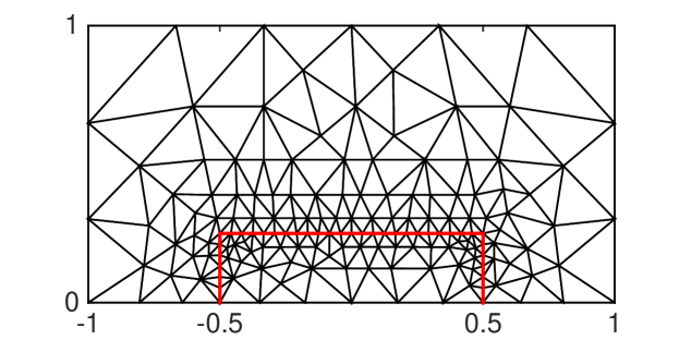
Figure 2: The initial computational mesh used in the convergence test with $J_{{}_{\Gamma}}=36$, $J_{\Omega}=166$ and $N=306$. The red line represents the fluid interface.

We first investigate the convergence of the proposed numerical method by carrying out simulations with different mesh sizes and time steps. The computational domain is $\Omega=[-1,1]\times[0,1]$ (i.e. $L_{x}=L_{y}=1$). Initially, the region occupied by fluid $1$ is the rectangle $\Omega_{1}(0)=[-0.5,0.5]\times[0,0.25]$. The parameters are chosen as $\rho_{1}=0.1$, $\beta_{1}=0.1$, $\eta_{1}=10$, $\beta^{*}=0.1$, $\theta_{Y}=2\pi/3$ and $Ca=0.01$.

Let $\mathbf{X}^{m}(\alpha)$ be the numerical solution for the interface at $t=t_{m}\ (m\geq 0)$ obtained with the time step $\tau$ and mesh size $h=1/J_{\Gamma}$. We define the approximate solution in any time interval $t_{m}\leq t<t_{m+1}$ using the linear interpolation:

$$\mathbf{X}_{h,\tau}(\alpha,t)=\frac{t-t_{m}}{\tau}\mathbf{X}^{m+1}(\alpha)+\frac{t_{m+1}-t}{\tau}\mathbf{X}^{m}(\alpha).$$ (4.1)

Then we measure the error of the numerical solution by comparing it with $\mathbf{X}_{\frac{h}{2},\frac{\tau}{4}}$, the numerical solution computed using refined mesh and time step,

$$e_{h,\tau}(t):=\max_{0\leq j\leq J_{{}_{\Gamma}}}\min_{\alpha\in[0,1]}\left|\mathbf{X}_{h,\tau}(\alpha_{j},t)-\mathbf{X}_{\frac{h}{2},\frac{\tau}{4}}(\alpha,t)\right|.$$ (4.2)

In Table. 1, we report the error of the numerical solution at the three different times $t=0.2,\ 1.0,\ 4.0$ for the two choices of elements P2-P0 and P2-(P1+P0), respectively. We observe that the error decreases with refined mesh size and time step. However, the order of convergence is unstable. This is due to the accumulation of the errors induced in the interpolations of the density and velocity fields, which are carried out at each time step.

Table 1: Error of the numerical solution and the rate of convergence for the fluid interface modelled using the Navier-Stokes equations. $h=1/J_{\Gamma}$ and $\tau$ are the mesh size in the discretization of the interface and the time step, respectively, where $h_{0}=1/36$ and $\tau_{0}=0.01$. The numerical results are obtained using the P2-P0 elements (upper panel) and the P2-(P1+P0) elements (lower panel).

  $(h,\ \tau)$ $e_{h,\tau}(t=0.2)$ order $e_{h,\tau}(t=1.0)$ order $e_{h,\tau}(t=4.0)$ order $(h_{0},\tau_{0})$ 5.86E-3 - 5.03E-3 - 5.75E-3 - $(\frac{h_{0}}{2},\frac{\tau_{0}}{2^{2}})$ 1.97E-3 1.57 1.07E-3 2.23 1.13E-3 2.35 $(\frac{h_{0}}{2^{2}},\frac{\tau_{0}}{2^{4}})$ 4.54E-4 2.12 5.74E-4 0.90 7.09E-4 0.67     $(h,\ \tau)$ $e_{h,\tau}(t=0.2)$ order $e_{h,\tau}(t=1.0)$ order $e_{h,\tau}(t=4.0)$ order $(h_{0},\tau_{0})$ 4.71E-3 - 4.28E-3 - 4.65E-3 - $(\frac{h_{0}}{2},\frac{\tau_{0}}{2^{2}})$ 1.58E-3 1.58 1.47E-3 1.54 1.74E-3 1.42 $(\frac{h_{0}}{2^{2}},\frac{\tau_{0}}{2^{4}})$ 4.25E-4 1.89 6.49E-4 1.18 8.18E-4 1.09  

Figure 3: The relative area change $\Delta V(t)$ of the droplet and the dynamic contact angle $\theta_{d}^{l}$ versus time for four different mesh sizes. The numerical results are obtained using the P2-P0 elements (upper panels) and the P2-(P1+P0) elements (lower panels).

Table 2: Convergence rates of $\Delta V$, the relative area change of the droplet, and $\theta_{d}^{l}$, the dynamic contact angle at $t=4$. $h$ and $\tau$ are the mesh size in the discretization of the interface and the time step, respectively, where $h_{0}=1/36$ and $\tau_{0}=0.01$. The numerical results are obtained using the P2-P0 elements (upper panel) and the P2-(P1+P0) elements (lower panel).

  $(h,\ \tau)$ $|\Delta V(t)|(t=4)$ order $|\theta_{d}^{l}(t)-\theta_{Y}|(t=4)$ order $(h_{0},\tau_{0})$ 2.28E-2 - 6.86E-2 - $(\frac{h_{0}}{2},\frac{\tau_{0}}{2^{2}})$ 6.38E-3 1.84 3.41E-2 1.01 $(\frac{h_{0}}{2^{2}},\frac{\tau_{0}}{2^{4}})$ 1.68E-3 1.93 1.70E-2 1.00 $(\frac{h_{0}}{2^{3}},\frac{\tau_{0}}{2^{6}})$ 4.28E-4 1.97 8.58E-3 0.99     $(h,\ \tau)$ $|\Delta V(t)|(t=4)$ order $|\theta_{d}^{l}(t)-\theta_{Y}|(t=4)$ order $(h_{0},\tau_{0})$ 2.31E-2 - 6.86E-2 - $(\frac{h_{0}}{2},\frac{\tau_{0}}{2^{2}})$ 6.44E-3 1.84 3.41E-2 1.01 $(\frac{h_{0}}{2^{2}},\frac{\tau_{0}}{2^{4}})$ 1.68E-3 1.94 1.70E-2 1.00 $(\frac{h_{0}}{2^{3}},\frac{\tau_{0}}{2^{6}})$ 4.28E-4 1.97 8.51E-3 1.00  

In Fig. 3, we present the relative area change of the droplet (left panels) and the dynamic contact angle (right panels) obtained using four different mesh sizes. The relative area change is defined as

$$\Delta V(t):=\frac{|\Omega_{1}(t)|-|\Omega_{1}(0)|}{|\Omega_{1}(0)|}.$$ (4.3)

As can be seen from the numerical results, by refining the mesh the area loss is significantly reduced for both pairs of elements. We also observe the convergence of the dynamic contact angle as the mesh is refined.

A more quantitative assessment for the area change and the contact angle is provided in Table  2, where we show the area change and the convergence of contact angle to its equilibrium value $\theta_{Y}=2\pi/3$ after the steady state is reached ($t=4$). We observe that both errors decrease as the mesh is refined. The convergence order for $\Delta V$ is about $2$, and the convergence order for $|\theta_{d}^{l}-\theta_{Y}|$ is about $1$. The later can be understood as follows. By choosing the test function $\boldsymbol{g}^{h}=(\phi_{0}(\alpha),~{}0)$ in (3.11d), where $\phi_{0}(\alpha)\in V^{h}$ is the piecewise linear function taking the value 1 at $\alpha_{0}=0$ and 0 at other nodes (i.e. the hat function at $\alpha_{0}$), we obtain

$$\frac{1}{2}\kappa^{m+1}(0)n_{1}^{m,1}\left|\mathbf{X}^{m}(\alpha_{1})-\mathbf{X}^{m}(\alpha_{0})\right|-\Bigl{(}\frac{\partial_{\alpha}\mathbf{X}^{m+1}}{|\partial_{\alpha}\mathbf{X}^{m}|}\Bigr{)}\Big{|}_{\alpha=0}+\cos\theta_{Y}+\frac{\beta^{*}Ca}{\tau_{m}}\left(x_{l}^{m+1}-x_{l}^{m}\right)=0.$$ (4.4)

At the steady state, we have $\mathbf{X}^{m+1}=\mathbf{X}^{m}$ and $\Bigl{(}\frac{\partial_{\alpha}\mathbf{X}^{m+1}}{|\partial_{\alpha}\mathbf{X}^{m}|}\Bigr{)}\Big{|}_{\alpha=0}=\partial_{s}\mathbf{X}^{m}\big{|}_{\alpha=0}=\cos\theta_{d}^{l,m}=\cos\theta_{d}^{l}$, thus,

$$\cos\theta_{d}^{l}-\cos\theta_{Y}=\frac{1}{2}\kappa_{h}(0)n_{1,h}^{1}\left|\mathbf{X}_{h}(\alpha_{1})-\mathbf{X}_{h}(\alpha_{0})\right|=O(\kappa_{h}(0)h),$$ (4.5)

where the subscript $h$ denotes the numerical solution at the steady state. This explains the order of convergence for the contact angle shown in Table 2.

We note that in this example (and examples below), the parameter $\alpha$ is chosen as the normalized arc length of the initial interface $\Gamma(0)$. Thus the mesh points are evenly distributed along $\Gamma(0)$. Since an implicit tangential velocity has been introduced for the interface evolution, and the mesh points tend to be uniformly distributed [53, 56], thus the quality of the mesh is well-preserved and no re-meshing is needed in the computation.

4.2 Numerical examples

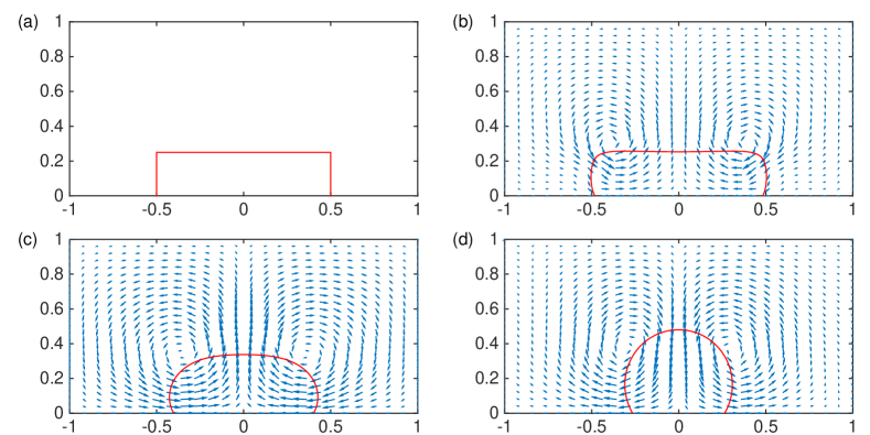
Figure 4: Snapshots of the interface and the velocity field modeled by two-phase Navier-Stokes equations, where $\theta_{Y}=2\pi/3$. (a) $t=0$: $\max\lVert\mathbf{u}\rVert_{0}=0$; (b) $t=0.1$: $\max\lVert\mathbf{u}\rVert_{0}=0.231$; (c) $t=0.5$: $\max\lVert\mathbf{u}\rVert_{0}=0.281$; (d) $t=2.0$: $\max\lVert\mathbf{u}\rVert_{0}=0.012$.

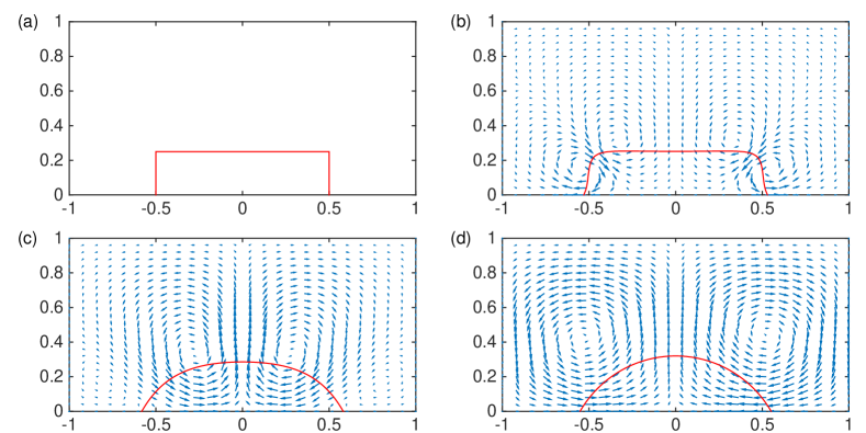
Figure 5: Snapshots of the interface and the velocity field modeled by two-phase Navier-Stokes equations, where $\theta_{Y}=\pi/3$. (a) $t=0$: $\max\lVert\mathbf{u}\rVert_{0}=0$; (b) $t=0.1$: $\max\lVert\mathbf{u}\rVert_{0}=0.305$; (c) $t=0.5$: $\max\lVert\mathbf{u}\rVert_{0}=0.075$; (d) $t=2.0$: $\max\lVert\mathbf{u}\rVert_{0}=0.002$.

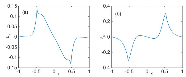
Figure 6: The slip velocity $u_{s}=\mathbf{u}\cdot\mathbf{t}_{w}$ at $t=0.1$. (a): the dewetting case with $\theta_{Y}=2\pi/3$; (b): the wetting case with $\theta_{Y}=\pi/3$.

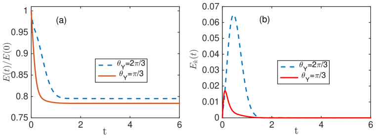
Figure 7: The normalized energy $E(t)/E(0)$ (left panel) and the kinetic energy $E_{k}(t):=\int_{\Omega}\frac{1}{2}\rho|\mathbf{u}|^{2}d\mathcal{L}^{2}$ (right panel) versus time.

Next we present two numerical examples. The first is similar to the one used in the convergence test but with different parameters, and the second is the transport of a droplet on solid substrate due to a surface tension gradient. The numerical results obtained using the P2-P0 elements and P2-(P1+P0) elements are indistinguishable in visualization, thus we will only present the results obtained using the P2-(P1+P0) elements.

Example 1. We first consider the evolution of a droplet on solid substrates with different equilibrium contact angles: $\theta_{Y}=\frac{2\pi}{3}$ and $\theta_{Y}=\frac{\pi}{3}$. The initial configuration of the droplet is given by a rectangle. The computational domain is $\Omega=[-1,1]\times[0,1]$, which is discretized by the triangular mesh with $N=3348$ triangles and $J_{\Omega}=1716$ vertices; the interface contains $J_{\Gamma}=120$ line segments. The time step is $\tau=5\times 10^{-4}$. Other parameters are chosen as $\rho_{1}=10$, $\beta_{1}=0.1$, $\eta_{1}=10$, $\beta^{*}=0.1$, and $Ca=0.1$.

Snapshots of the interface and the velocity field at several times are shown in Fig. 4 and Fig. 5 for the two cases , respectively. In both cases, we can clearly observe the development of a pair of vortices in the velocity field associated with the evolution of the interface. In the dewetting case ($\theta_{Y}=2\pi/3$), inward velocities are generated at the contact points due to the unbalanced Young stress, causing the contact points to retreat so that the contact angle converges to its equilibrium value. On the other hand, outward velocities are generated at the contact points in the wetting case ($\theta_{Y}=\pi/3$), which drives the droplet to spread on the substrate. The slip velocities along the substrate at time $t=0.1$ are shown in Fig. 6. We can observe that the slip velocity takes the maximal value (in magnitude) at the contact points in both cases.

In Fig. 7, we show the total and kinetic energies against time. In particular, we observe the decay of the total energy in time.

Example 2. We next consider the migration of a droplet on a solid substrate with surface tension gradients. The equilibrium contact angle $\theta_{Y}$ depends on the position of the contact point:

$$\cos\theta_{Y}(x)=\left\{\begin{array}[]{ll}-0.8,&\quad\mbox{for}\ x<-0.8,\\ x,&\quad\mbox{for}\ -0.8\leq x<0.8,\\ 0.8,&\quad\mbox{for}\ x\geq 0.8.\end{array}\right.$$ (4.6)

The initial configuration of the droplet is given by the rectangle $[-0.5,-0.25]\times[0,0.25]$. The triangular mesh consists of $N=3036$ triangles and $J_{\Omega}=1580$ vertices. The interface contains $J_{\Gamma}=60$ vertices. The time step is $\tau=2\times 10^{-4}$. Other parameters are chosen as $\rho_{1}=1$, $\beta_{1}=0.1$, $\eta_{1}=0.1$, $\beta^{*}=0.1$ and $Ca=0.1$.

The profiles of the droplet at several times are shown in Fig. 8. From the figure, we observe that the droplet first evolves into a nearly spherical configuration, then migrates along the substrate from the region with lower value of $\cos\theta_{Y}$ to the region with higher value of $\cos\theta_{Y}$ in order to lower the interfacial energy on the solid surface. The decay of the energy is shown in Fig. 9. In the figure we also show the area of the droplet and the contact angles versus time. We can see that the area is very well preserved.

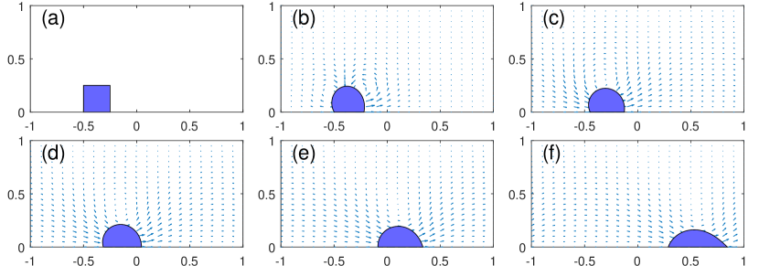
Figure 8: Snapshots of the droplet migrating on a substrate with surface tension gradient. (a) $t=0$; (b) $t=0.1$; (c) $t=0.4$; (d) $t=0.8$; (e) $t=1.3$; (f) $t=1.9$.

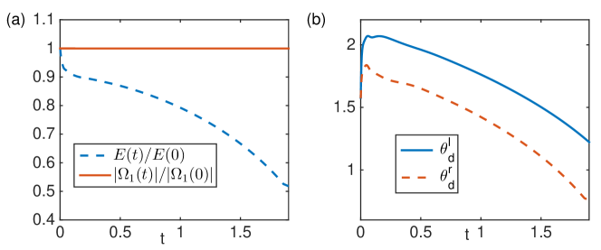
Figure 9: (a) The normalized energy $E(t)/E(0)$ and the relative area $|\Omega 1(t)|/|\Omega_{1}(0)|$ versus time; (b) The dynamic contact angles versus time.

5 Stokes flow

In this section, we consider the case in which the Reynolds number is small so that the flow is modeled by the time-independent Stokes equations in $\Omega_{i}\ (i=1,2)$,

$$\nabla p-\nabla\cdot\tau_{d}=0,$$ (5.1a)

$$\nabla\cdot\mathbf{u}=0,$$ (5.1b)

with the interface conditions on $\Gamma$,

$$\bigl{[}\mathbf{u}\bigr{]}^{2}_{1}=0,$$ (5.2a)

$$Ca\,\bigl{[}\sigma\bigr{]}_{1}^{2}\cdot\mathbf{n}=\kappa\,\mathbf{n},$$ (5.2b)

$$\kappa=(\partial_{ss}\mathbf{X})\cdot\mathbf{n},$$ (5.2c)

$$\dot{\mathbf{x}}_{\Gamma}=\mathbf{u}|_{\mathbf{x}_{\Gamma}},$$ (5.2d)

and the same boundary and dynamic contact angle conditions as in (2.10) - (2.13), where $\sigma=p\mathbf{I}-\tau_{d}$. Below we present the corresponding finite element method and conduct convergence tests.

5.1 The finite element method

The numerical method is similar to the one introduced in section 3.1. At the $m$-th time step, given a triangulation of $\Omega_{1}\cup\Omega_{2}$, $\mathcal{T}^{m}$, which is fitted to the interface $\Gamma^{m}$, we solve the following linear system for $\mathbf{u}^{m+1}\in\mathbb{U}^{m}$, $p^{m+1}\in\hat{\mathbb{P}}^{m}$, $\mathbf{X}^{m+1}\in V^{h}\times V^{h}_{0}$, and $\kappa^{m+1}\in V^{h}$,

$$-\Bigl{(}p^{m+1},~{}\nabla\cdot\boldsymbol{\omega}^{h}\bigr{)}+2\,\Bigl{(}\eta^{m}D(\mathbf{u}^{m+1}),~{}D(\boldsymbol{\omega}^{h})\Bigr{)}$$

$$\qquad\qquad-\;\frac{1}{Ca}\Bigl{(}\kappa^{m+1}\,\mathbf{n}^{m},~{}\boldsymbol{\omega}^{h}\Bigr{)}_{\Gamma^{m}}+\;\frac{1}{l_{s}}\Bigr{(}\beta^{m}\,u_{s}^{m+1},~{}\omega_{s}^{h}\Bigr{)}_{\Gamma_{1}^{m}\cup\Gamma_{2}^{m}}=0,\quad\forall\boldsymbol{\omega}^{h}\in\mathbb{U}^{m},$$ (5.3a)

$$\qquad\qquad\qquad\qquad\qquad\Bigl{(}\nabla\cdot\mathbf{u}^{m+1},~{}q^{h}\Bigr{)}=0,\qquad\forall q^{h}\in\hat{\mathbb{P}}^{m}.$$ (5.3b)

$$\qquad\frac{1}{\tau_{m}}\Bigl{(}(\mathbf{X}^{m+1}-\mathbf{X}^{m})\cdot\mathbf{n}^{m},~{}\psi^{h}\Bigr{)}_{\Gamma^{m}}^{h}-\Bigl{(}\mathbf{u}^{m+1}\cdot\mathbf{n}^{m},~{}\psi^{h}\Bigr{)}_{\Gamma^{m}}=0,\quad\forall\psi^{h}\in V^{h}.$$ (5.3c)

$$\Bigl{(}\kappa^{m+1}\,\mathbf{n}^{m},~{}\boldsymbol{g}^{h}\Bigr{)}_{\Gamma^{m}}^{h}+\Bigl{(}\partial_{s}\mathbf{X}^{m+1},~{}\partial_{s}\boldsymbol{g}^{h}\Bigr{)}_{\Gamma^{m}}-\cos\theta_{Y}\,[g_{1}^{h}(1)-g_{1}^{h}(0)]$$

$$\qquad\quad+\frac{\beta^{*}\,Ca}{\tau_{m}}\Bigl{[}(x^{m+1}_{r}-x^{m}_{r})g_{1}^{h}(1)+(x^{m+1}_{l}-x_{l}^{m})g_{1}^{h}(0)\Bigr{]}=0,\quad\forall\boldsymbol{g}^{h}\in V^{h}\times V^{h}_{0}.$$ (5.3d)

Then we update the triangular mesh $\mathcal{T}^{m}$ using the method introduced in section 3.3 so that it fits to the new interface $\Gamma^{m+1}$, and the above procedure repeats.

We can show the numerical scheme Eq. (5.3)-Eq. (5.3d) admits a unique solution (Theorem 5.3) and satisfies a discrete energy law (Theorem 5.4).

Theorem 5.3 (Well-posedness).

Let $(\mathbb{U}^{m},~{}\hat{\mathbb{P}}^{m})$ satisfy the inf-sup stability condition (3.10) and the interface $\mathbf{X}^{m}(\cdot)$ satisfy the conditions in (3.5). Then the numerical methods (5.3)-(5.3d), admits a unique solution.

The proof is similar to the proof of Theorem 3.1, so is omitted.

Theorem 5.4 (Stability bound).

Let $\Bigl{(}\mathbf{u}^{m+1},~{}p^{m+1},~{}\mathbf{X}^{m+1},~{}\kappa^{m+1}\Bigr{)}$ be the solution to the numerical scheme (5.3)-(5.3d). Then the following stability bound holds

$$-\frac{\cos\theta_{Y}}{Ca}|\Gamma_{1}^{m+1}|+\frac{1}{Ca}|\Gamma^{m+1}|+2\tau_{m}\lVert\sqrt{\eta^{m}}D(\mathbf{u}^{m+1})\rVert_{0}^{2}+\frac{\tau_{m}}{l_{s}}\Bigl{(}\beta^{m}\,u_{s}^{m+1},~{}u_{s}^{m+1}\Bigr{)}_{\Gamma^{m}_{1}\cup\Gamma_{2}^{m}}$$

$$\qquad\qquad+\frac{\beta^{*}}{\tau_{m}}\Bigl{[}(x^{m+1}_{r}-x^{m}_{r})^{2}+(x^{m+1}_{l}-x^{m}_{l})^{2}\Bigr{]}\leq-\frac{\cos\theta_{Y}}{Ca}|\Gamma_{1}^{m}|+\frac{1}{Ca}|\Gamma^{m}|.$$ (5.4)

Moreover, for $k\geq 1$, we have

$$-\frac{\cos\theta_{Y}}{Ca}|\Gamma_{1}^{k}|+\frac{1}{Ca}|\Gamma^{k}|+\sum_{m=0}^{k-1}2\tau_{m}\lVert\sqrt{\eta^{m}}D(\mathbf{u}^{m+1})\rVert_{0}^{2}+\sum_{m=0}^{k-1}\frac{\tau_{m}}{l_{s}}\Bigl{(}\beta^{m}\,u_{s}^{m+1},~{}u_{s}^{m+1}\Bigr{)}_{\Gamma^{m}_{1}\cup\Gamma_{2}^{m}}$$

$$\qquad\qquad+\sum_{m=0}^{k-1}\frac{\beta^{*}}{\tau_{m}}\Bigl{[}(x^{m+1}_{r}-x^{m}_{r})^{2}+(x^{m+1}_{l}-x^{m}_{l})^{2}\Bigr{]}\leq-\frac{\cos\theta_{Y}}{Ca}|\Gamma_{1}^{0}|+\frac{1}{Ca}|\Gamma^{0}|.$$ (5.5)

Proof.

Choosing $\boldsymbol{\omega}^{h}=\mathbf{u}^{m+1}$, $q^{h}=p^{m+1}$, $\psi^{h}=\frac{1}{Ca}\kappa^{m+1}$ and $\boldsymbol{g}^{h}=\frac{1}{Ca}(\mathbf{X}^{m+1}-\mathbf{X}^{m})$ in (5.3)-(5.3d), then combining the equations yields

$$2\Bigl{(}\eta^{m}D(\mathbf{u}^{m+1}),~{}D(\mathbf{u}^{m+1})\Bigr{)}+\frac{1}{l_{s}}\left(\beta^{m}\,u_{s}^{m+1},~{}u_{s}^{m+1}\right)_{\Gamma_{1}^{m}\cup\Gamma_{2}^{m}}+\frac{1}{Ca\cdot\tau_{m}}\Bigl{(}\partial_{s}\mathbf{X}^{m+1},~{}\partial_{s}(\mathbf{X}^{m+1}-\mathbf{X}^{m})\Bigr{)}_{\Gamma^{m}}$$

$$-\frac{\cos\theta_{Y}}{Ca\cdot\tau_{m}}\Bigl{[}(x_{r}^{m+1}-x_{l}^{m+1})-(x_{r}^{m}-x_{l}^{m})\Bigr{]}+\frac{\beta^{*}}{(\tau_{m})^{2}}\Bigl{[}(x_{r}^{m+1}-x_{r}^{m})^{2}+(x_{l}^{m+1}-x_{l}^{m})^{2}\Bigr{]}=0.$$ (5.6)

Eq. (5.4) immediately follows by noting Eq. (3.22). By summing up Eq. (5.4) for $m$ from $0$ to $k-1$, we obtain the energy dissipation law Eq. (5.5). ∎

In contrast to the numerical scheme in (3.11)-(3.11d) for the Navier-Stokes equations, the interpolation step of the velocity and density fields from $\mathcal{T}^{m}$ to the new mesh $\mathcal{T}^{m+1}$ is not needed for Stokes flow. This allowed us to prove the global energy dissipation law in (5.5). Similar work for the two-phase Stokes flow without contact lines has been done in Ref. [52]; there the method was shown to be unconditionally stable.

Table 3: Error of the numerical solution and the rate of convergence for the fluid interface modeled using the Stokes equations. $h=1/J_{\Gamma}$ and $\tau$ are the mesh size and the time step, respectively, where $h_{0}=1/36$ and $\tau_{0}=0.01$. The numerical results are obtained using the P2-P0 elements (upper panel) and the P2-(P1+P0) elements (lower panel).

  $(h,\ \tau)$ $e_{h,\tau}(t=0.2)$ order $e_{h,\tau}(t=1.0)$ order $e_{h,\tau}(t=4.0)$ order $(h_{0},\tau_{0})$ 4.10E-3 - 4.20E-3 - 4.19E-3 - $(\frac{h_{0}}{2},\frac{\tau_{0}}{2^{2}})$ 1.15E-3 1.83 1.20E-3 1.81 1.20E-3 1.80 $(\frac{h_{0}}{2^{2}},\frac{\tau_{0}}{2^{4}})$ 3.08E-4 1.90 3.23E-4 1.89 3.22E-4 1.90     $(h,\ \tau)$ $e_{h,\tau}(t=0.2)$ order $e_{h,\tau}(t=1.0)$ order $e_{h,\tau}(t=4.0)$ order $(h_{0},\tau_{0})$ 4.13E-3 - 4.15E-3 - 4.13E-3 - $(\frac{h_{0}}{2},\frac{\tau_{0}}{2^{2}})$ 1.18E-3 1.81 1.18E-3 1.81 1.18E-3 1.81 $(\frac{h_{0}}{2^{2}},\frac{\tau_{0}}{2^{4}})$ 3.13E-4 1.91 3.16E-4 1.90 3.15E-4 1.91  

5.2 Convergence test

We investigate the accuracy and the convergence rate of the numerical method using the same example in section 4.1, with the parameters $\beta_{1}=0.1$, $\eta_{1}=10$, $\beta^{*}=0.1$, $\theta_{Y}=2\pi/3$, $l_{s}=0.1$ and $Ca=0.01$. The numerical results are summarized in Table. 3, where the errors of the fluid interface are computed using Eq. (4.2). We can clearly observe the convergence for both P2-P0 and P2-(P1+P0) elements. The convergence rates approach 2 as the mesh is refined.

6 Conclusions

In this work, we have developed an efficient energy-stable numerical method for two-phase fluids with moving contact lines. The method combines the finite element method for the Navier-Stokes/Stokes equations with a semi-implicit parametric finite element method for the dynamics of the fluid interface. We used the moving mesh approach such that the evolving fluid interface remains fitted to the triangular mesh. At each time step, the new mesh is constructed based on the mesh at the previous time step by solving an elastic equation with proper boundary conditions for the displacements of the internal nodes.

The contact line condition in the model relates the dynamic contact angle of the interface to the contact line velocity. It is a non-trivial task to properly impose this condition in numerical simulations. In this work, we formulated it as a time-dependent Robin-type of boundary condition for the fluid interface so it is naturally imposed in the weak form of the governing equations.

For the Navier-Stokes equations, we showed that the numerical scheme obeys a similar energy law as the continuum model but up to an error due to the interpolation of the numerical solutions on the moving mesh. For Stokes flow, the interpolation is not needed so we were able to prove the global unconditional stability in terms of the energy. Numerical simulations have demonstrated the convergence and accuracy of the numerical methods. For Stokes flows, the convergence rate for the interface dynamics reaches about 2 as the mesh is refined. However, for Navier-Stokes equations, the numerical solution is polluted by the interpolation error, and the order of convergence is unstable.

The current work focused on systems in two dimensions. In the future, we intend to extend the numerical method to systems in three dimensions and also more challenging problems such electro-wetting, contact line dynamics on elastic substrate, etc.

Reference

References

- [1] C. Huh, L. E. Scriven, Hydrodynamic model of steady movement of a solid/liquid/fluid contact line, J. Colloid Interface Sci. 35 (1971) 85–101.
- [2] E. B. Dussan V, S. H. Davis, On the motion of a fluid-fluid interface along a solid surface, J. Fluid Mech. 65 (1974) 71–95.
- [3] J. Koplik, J. R. Banavar, J. F. Willemsen, Molecular dynamics of poiseuille flow and moving contact lines, Phys. Rev. Lett. 60 (13) (1988) 1282–1285.
- [4] P. A. Thompson, M. O. Robbins, Simulations of contact-line motion: slip and the dynamics contact angle, Phys. Rev. Lett. 63 (7) (1989) 766–769.
- [5] W. Ren, W. E, Boundary conditions for the moving contact line problem, Phys. Fluids. 19 (2) (2007) 022101.
- [6] J. De Coninck, T. D. Blake, Wetting and molecular dynamics simulations of simple liquids, Annu. Rev. Mater. Res. 38 (2008) 1–22.
- [7] T. D. Blake, J. M. Haynes, Kinetics of liquid/liquid displacement, J. Colloid Interface Sci. 30 (3) (1969) 421–423.
- [8] T. D. Blake, Dynamic contact angles and wetting kinetics, in: Wettability, Vol. 49 of Surfactant Science Series, Marcel Dekker, 1993, p. 251.
- [9] D. M. Anderson, G. B. McFadden, A. A. Wheeler, Diffuse-interface methods in fluid mechanics, Annu. Rev. Fluid Mech. 30 (1) (1998) 139–165.
- [10] D. Jacqmin, Contact-line dynamics of a diffuse fluid interface, J. Fluid Mech. 402 (1) (2000) 57–88.
- [11] L. M. Pismen, Mesoscopic hydrodynamics of contact line motion, Colloids Surf. A 206 (1) (2002) 11–30.
- [12] T. Qian, X.-P. Wang, P. Sheng, Molecular scale contact line hydrodynamics of immiscible flows, Phys. Rev. E. 68 (1) (2003) 016306.
- [13] P. Yue, C. Zhou, J. J. Feng, Sharp interface limit of the cahn-hilliard model for moving contact lines, J. Fluid Mech. 645 (2010) 279–294.
- [14] Y. D. Shikhmurzaev, Moving contact lines in liquid/liquid/solid systems, J. Fluid Mech. 334 (1) (1997) 211–249.
- [15] O. V. Voinov, Hydrodynamics of wetting, Fluid Dyn. 11 (5) (1976) 714–721.
- [16] L. M. Hocking, A moving fluid interface. part 2. the removal of the force singularity by a slip flow, J. Fluid Mech. 79 (1977) 209.
- [17] R. G. Cox, The dynamics of the spreading of liquids on a solid surface. part 1. viscous flow, J. Fluid Mech. 168 (1986) 169–194.
- [18] J. Eggers, Hydrodynamic theory of forced dewetting, Phys. Rev. Lett. 93 (9) (2004a) 094502.
- [19] W. Ren, D. Hu, W. E, Continuum models for the contact line problem, Phys. Fluids. 22 (2010) 102103.
- [20] W. Ren, E. Weinan, Derivation of continuum models for the moving contact line problem based on thermodynamic principles, Commun Math Sci. 9 (2) (2011) 597–606.
- [21] W. Ren, P. H. Trinh, W. E, On the distinguished limits of the navier slip model of the moving contact line problem, J. Fluid Mech. 772 (2015) 107–126.
- [22] Z. Zhang, W. Ren, Distinguished limits of the navier slip model for moving contact lines in stokes flow, SIAM J. Appl. Math. 79 (2019) 1654–1674.
- [23] D. N. Sibley, A. Nold, S. Kalliadasis, The asymptotics of the moving contact line:cracking an old nut, J. Fluid Mech. 764 (2015) 445–462.
- [24] E. B. Dussan V, On the spreading of liquids on solid surfaces: Static and dynamic contact lines, Annu. Rev. Fluid Mech. 11 (1979) 371.
- [25] P. G. de Gennes, Wetting: Statics and dynamics, Rev. Mod. Phys. 57 (1985) 827–863.
- [26] S. F. Kistler, Hydrodynamics of wetting, in: Wettability, Vol. 49 of Surfactant Science Series, Marcel Dekker, 1993, pp. 311–430.
- [27] Y. Pomeau, Recent progress in the moving contact line problem: a review, C. R. Mecanique 330 (2002) 207–222.
- [28] D. Bonn, J. Eggers, J. Indekeu, J. Meunier, E. Rolley, Wetting and spreading, Rev. Mod. Phys. 81 (2009) 739.
- [29] M. G. Velarde, Discussion and debate: Wetting and spreading science - quo vadis?, Eur. Phys. J. Special Top. 197 (1) (2011) 1–343.
- [30] P. G. de Gennes, F. Brochard-Wyart, D. Quéré, Capillay and wetting phenomena: Drops, bubbles, pearls, waves, Springer, New York, 2003.
- [31] V. M. Starov, M. G. Velarde, C. J. Radke, Wetting and spreading dynamics, CRC press, 2007.
- [32] S. Afkhami, S. Zaleski, M. Bussmann, A mesh-dependent model for applying dynamic contact angles to VOF simulations, J. Conmput. Phys. 228 (15) (2009) 5370–5389.
- [33] M. Renardy, Y. Renardy, J. Li, Numerical simulation of moving contact line problems using a volume-of-fluid method, J. Comput. Phys. 171 (1) (2001) 243–263.
- [34] J.-B. Dupont, D. Legendre, Numerical simulation of static and sliding drop with contact angle hysteresis, J. Comput. Phys. 229 (7) (2010) 2453–2478.
- [35] Z. Li, M.-C. Lai, G. He, H. Zhao, An augmented method for free boundary problems with moving contact lines, Comput & Fluids 39 (6) (2010) 1033–1040.
- [36] W. Ren, W. E, Contact line dynamics on heterogeneous surfaces, Phys. Fluids 23 (7) (2011) 072103.
- [37] P. D. Spelt, A level-set approach for simulations of flows with multiple moving contact lines with hysteresis, J. Comput. Phys. 207 (2) (2005) 389–404.
- [38] S. Zahedi, K. Gustavsson, G. Kreiss, A conservative level set method for contact line dynamics, J. Comput. Phys. 228 (17) (2009) 6361–6375.
- [39] J.-J. Xu, W. Ren, A level-set method for two-phase flows with moving contact line and insoluble surfactant, J. Comput. Phys. 263 (2014) 71–90.
- [40] S. Xu, W. Ren, Reinitialization of the level-set function in 3d simulation of moving contact lines, Commun. Comput. Phys. 20 (5) (2016) 1163–1182.
- [41] M. Gao, X.-P. Wang, An efficient scheme for a phase field model for the moving contact line problem with variable density and viscosity, J. Comput. Phys. 272 (2014) 704–718.
- [42] K. Bao, Y. Shi, S. Sun, X.-P. Wang, A finite element method for the numerical solution of the coupled Cahn–Hilliard and Navier–Stokes system for moving contact line problems, J. Comput. Phys. 231 (24) (2012) 8083–8099.
- [43] H. Ding, P. D. Spelt, Onset of motion of a three-dimensional droplet on a wall in shear flow at moderate Reynolds numbers, J. Fluid Mech 599 (2008) 341–362.
- [44] A. Carlson, M. Do-Quang, G. Amberg, Modeling of dynamic wetting far from equilibrium, Phys. Fluids. 21 (12) (2009) 121701.
- [45] Z. Zhang, W. Ren, Simulation of moving contact lines in two-phase polymeric fluids, Computers & Mathematics with Applications 72 (4) (2016) 1002–1012.
- [46] H. Huang, D. Liang, B. Wetton, Computation of a moving drop/bubble on a solid surface using a front-tracking method, Commun. Math. Sci. 2 (4) (2004) 535–552.
- [47] M. Muradoglu, S. Tasoglu, A front-tracking method for computational modeling of impact and spreading of viscous droplets on solid walls, Comput & Fluids 39 (4) (2010) 615–625.
- [48] Z. Zhang, S. Xu, W. Ren, Derivation of a continuum model and the energy law for moving contact lines with insoluble surfactants, Phys. Fluids 26 (2014) 062103.
- [49] Y. Sui, H. Ding, P. D. Spelt, Numerical simulations of flows with moving contact lines, Annu. Rev. Fluid Mech. 46 (1) (2014) 97–119.
- [50] J. W. Barrett, H. Garcke, R. Nürnberg, A stable parametric finite element discretization of two-phase Navier–Stokes flow, J. Sci. Comput. 63 (1) (2015) 78–117.
- [51] J. W. Barrett, H. Garcke, R. Nürnberg, On the stable numerical approximation of two-phase flow with insoluble surfactant, ESAIM: Math Model Num Anal. 49 (2) (2015) 421–458.
- [52] M. Agnese, R. Nürnberg, Fitted finite element discretization of two-phase Stokes flow, Int J Numer Methods Fluids. 82 (11) (2016) 709–729.
- [53] J. W. Barrett, H. Garcke, R. Nürnberg, A parametric finite element method for fourth order geometric evolution equations, J. Comput. Phys 222 (1) (2007) 441–467.
- [54] A. Masud, T. J. Hughes, A space-time Galerkin/least-squares finite element formulation of the Navier-Stokes equations for moving domain problems, Comput. Methods Appl. Mech. Eng. 146 (1-2) (1997) 91–126.
- [55] J. Liu, A second-order changing-connectivity ALE scheme and its application to FSI with large convection of fluids and near contact of structures, J. Comput. Phys. 304 (2016) 380–423.
- [56] W. Bao, W. Jiang, Y. Wang, Q. Zhao, A parametric finite element method for solid-state dewetting problems with anisotropic surface energies, J. Comput. Phys. 330 (2017) 380–400.