Squashed Shifted PMI Matrix: Bridging Word Embeddings and Hyperbolic Spaces

Abstract

We show that removing sigmoid transformation in the skip-gram with negative sampling (SGNS) objective does not harm the quality of word vectors significantly and at the same time is related to factorizing a squashed shifted PMI matrix which, in turn, can be treated as a connection probabilities matrix of a random graph. Empirically, such graph is a complex network, i.e. it has strong clustering and scale-free degree distribution, and is tightly connected with hyperbolic spaces. In short, we show the connection between static word embeddings and hyperbolic spaces through the squashed shifted PMI matrix using analytical and empirical methods.

1 Introduction

Modern word embedding models (McCann et al., 2017; Peters et al., 2018; Devlin et al., 2019) build vector representations of words in context, i.e. the same word will have different vectors when used in different contexts (sentences). Earlier models (Mikolov et al., 2013b; Pennington et al., 2014) built the so-called static embeddings: each word was represented by a single vector, regardless of the context in which it was used.

Despite the fact that static word embeddings are considered obsolete today, they have several advantages compared to contextualized ones. Firstly, static embeddings are trained much faster (few hours instead of few days) and do not require large computing resources (1 consumer-level GPU instead of 8–16 non-consumer GPUs). Secondly, they have been studied theoretically in a number of works (Levy and Goldberg, 2014b; Arora et al., 2016; Hashimoto et al., 2016; Gittens et al., 2017; Tian et al., 2017; Ethayarajh et al., 2019; Allen et al., 2019; Allen and Hospedales, 2019; Assylbekov and Takhanov, 2019; Zobnin and Elistratova, 2019) but not much has been done for the contextualized embeddings (Reif et al., 2019). Thirdly, static embeddings are still an integral part of deep neural network models that produce contextualized word vectors, because embedding lookup matrices are used at the input and output (softmax) layers of such models. Therefore, we consider it necessary to further study static embeddings.

With all the abundance of both theoretical and empirical studies on static vectors, they are not fully understood, as this work shows. For instance, it is generally accepted that good quality word vectors are inextricably linked with a low-rank approximation of the pointwise mutual information (PMI) matrix or the Shifted PMI (SPMI) matrix, but we show that vectors of comparable quality can also be obtained from a low-rank approximation of a Squashed SPMI matrix (Section 2). Thus, a Squashed SPMI matrix is a viable alternative to standard PMI/SPMI matrices when it comes to obtaining word vectors.

At the same time, it is easy to interpret the Squashed SPMI matrix with entries in $[0,1)$ as a connection probabilities matrix for generating a random graph. Studying the properties of such a graph, we come to the conclusion that it is a so-called complex network, i.e. it has a strong clustering property and a scale-free degree distribution (Section 3).

It is noteworthy that complex networks, in turn, are dual to hyperbolic spaces (Section 4) as was shown by Krioukov et al. (2010). Hyperbolic geometry has been used to train word vectors (Nickel and Kiela, 2017; Tifrea et al., 2018) and has proven its suitability — in a hyperbolic space, word vectors need lower dimensionality than in the Euclidean space.

Thus, to the best of our knowledge, this is the first work that establishes simultaneously a connection between word vectors, a Squashed SPMI matrix, complex networks, and hyperbolic spaces. Figure 1 summarizes our work and serves as a guide for the reader.

Figure 1: Summary of our work

Notation

We let $\mathbb{R}$ denote the real numbers. Bold-faced lowercase letters ($\mathbf{x}$) denote vectors, plain-faced lowercase letters ($x$) denote scalars, $\langle\mathbf{x},\mathbf{y}\rangle$ is the Euclidean inner product, $(a_{ij})$ is a matrix with the $ij$-th entry being $a_{ij}$. ‘i.i.d.’ stands for ‘independent and identically distributed’. We use the sign $\propto$ to abbreviate ‘proportional to’, and the sign $\sim$ to abbreviate ‘distributed as’.

Assuming that words have already been converted into indices, let $\mathcal{W}:=\{1,\ldots,n\}$ be a finite vocabulary of words. Following the setup of the widely used word2vec model (Mikolov et al., 2013b), we use two vectors per each word $i$: (1) $\mathbf{w}_{i}\in\mathbb{R}^{d}$ when $i\in\mathcal{W}$ is a center word, (2) $\mathbf{c}_{i}\in\mathbb{R}^{d}$ when $i\in\mathcal{W}$ is a context word; and we assume that $d\ll n$.

In what follows we assume that our dataset consists of co-occurence pairs $(i,j)$. We say that “the words $i$ and $j$ co-occur” when they co-occur in a fixed-size window of words. The number of such pairs, i.e. the size of our dataset, is denoted by $N$. Let $\#(i,j)$ be the number of times the words $i$ and $j$ co-occur, then $N=\sum_{i\in\mathcal{W}}\sum_{j\in\mathcal{W}}\#(i,j)$.

2 Squashed SPMI and Word Vectors

A well known skip-gram with negative sampling (SGNS) word embedding model of Mikolov et al. (2013b) maximizes the following objective function

$$\textstyle\sum_{i\in\mathcal{W}}\sum_{j\in\mathcal{W}}\#(i,j)\left(\log\sigma(\langle\mathbf{w}_{i},\mathbf{c}_{j}\rangle)+k\cdot\mathbb{E}_{j^{\prime}\sim p}[\log\sigma(-\langle\mathbf{w}_{i},\mathbf{c}_{j^{\prime}}\rangle)]\right),$$ (1)

where $\sigma(x)=\frac{1}{1+e^{-x}}$ is the logistic sigmoid function, $p$ is a smoothed unigram probability distribution for words, and $k$ is the number of negative samples to be drawn. Interestingly, training SGNS is approximately equivalent to finding a low-rank approximation of a Shifted PMI matrix (Levy and Goldberg, 2014b) in the form $\log\frac{p(i,j)}{p(i)p(j)}-\log k\approx\langle\mathbf{w}_{i},\mathbf{c}_{j}\rangle$, where the left-hand side is the $ij$-th element of the $n\times n$ shifted PMI matrix, and the right-hand side is an element of a matrix with rank $\leq d$ since $\mathbf{w}_{i},\mathbf{c}_{j}\in\mathbb{R}^{d}$. This approximation (up to a constant shift) was later re-derived by Arora et al. (2016); Assylbekov and Takhanov (2019); Allen et al. (2019); Zobnin and Elistratova (2019) under different sets of assuptions. In this section we show that constraint optimization of a slightly modified SGNS objective (1) leads to a low-rank approximation of the Squashed Shifted PMI ($\sigma$SPMI) matrix, defined as $\sigma\mathrm{SPMI}_{ij}:=\sigma(\mathrm{PMI}_{ij}-\log k)$.

Theorem 2.1

Assuming $0<\langle\mathbf{w}_{i},\mathbf{c}_{j}\rangle<1$, the following objective function

$$\mathcal{L}=\sum_{i\in\mathcal{W}}\sum_{j\in\mathcal{W}}\underbrace{\#(i,j)\left(\log\langle\mathbf{w}_{i},\mathbf{c}_{j}\rangle+k\cdot\mathbb{E}_{j^{\prime}\sim P}[\log(1-\langle\mathbf{w}_{i},\mathbf{c}_{j^{\prime}}\rangle)]\right)}_{\ell(\mathbf{w}_{i},\mathbf{c}_{j})},$$ (2)

reaches its optimum at $\langle\mathbf{w}_{i},\mathbf{c}_{j}\rangle=\sigma\mathrm{SPMI}_{ij}$.

Proof

Expanding the sum and the expected value in (2) as in Levy and Goldberg (2014b), and defining $p(i,j):=\frac{\#(i,j)}{N}$, $p(i):=\frac{\#(i)}{N}$, we have

$$\mathcal{L}=N\sum_{i\in\mathcal{W}}\sum_{j\in\mathcal{W}}p(i,j)\cdot\log\langle\mathbf{w}_{i},\mathbf{c}_{j}\rangle+p(i)\cdot p(j)\cdot k\cdot\log(1-\langle\mathbf{w}_{i},\mathbf{c}_{j}\rangle).$$ (3)

Thus, we can rewrite the individual objective $\ell(\mathbf{w}_{i},\mathbf{c}_{j})$ in (2) as

$$\ell=N\left[p(i,j)\cdot\log\langle\mathbf{w}_{i},\mathbf{c}_{j}\rangle+p(i)\cdot p(j)\cdot k\cdot\log(1-\langle\mathbf{w}_{i},\mathbf{c}_{j}\rangle)\right].$$ (4)

Differentiating (4) w.r.t. $\langle\mathbf{w}_{i},\mathbf{c}_{j}\rangle$ we get

$$\frac{\partial\ell}{\partial\langle\mathbf{w}_{i},\mathbf{c}_{j}\rangle}=N\left[\frac{p(i,j)}{\langle\mathbf{w}_{i},\mathbf{c}_{j}\rangle}-\frac{p(i)\cdot p(j)\cdot k}{1-\langle\mathbf{w}_{i},\mathbf{c}_{j}\rangle}\right].$$

Setting this derivative to zero gives

$$\frac{p(i,j)}{p(i)p(j)}\cdot\frac{1}{k}=\frac{\langle\mathbf{w}_{i},\mathbf{c}_{j}\rangle}{1-\langle\mathbf{w}_{i},\mathbf{c}_{j}\rangle}\quad\Rightarrow\quad\log\frac{p(i,j)}{p(i)p(j)}-\log k=\log\frac{\langle\mathbf{w}_{i},\mathbf{c}_{j}\rangle}{1-\langle\mathbf{w}_{i},\mathbf{c}_{j}\rangle}\\ \Leftrightarrow\quad\log\frac{p(i,j)}{p(i)p(j)}-\log k=\operatorname*{logit}\langle\mathbf{w}_{i},\mathbf{c}_{j}\rangle\\ \Leftrightarrow\quad\sigma\left(\log\frac{p(i,j)}{p(i)p(j)}-\log k\right)=\langle\mathbf{w}_{i},\mathbf{c}_{j}\rangle,$$ (5)

where $\operatorname*{logit}(q):=\log\frac{q}{1-q}$ is the logit function which is the inverse of the logistic sigmoid function, i.e. $\sigma(\operatorname*{logit}(q))=q$. From (5) we have $\sigma\mathrm{SPMI}_{ij}=\langle\mathbf{w}_{i},\mathbf{c}_{j}\rangle$, which concludes the proof.

Remark 1

Since $\sigma(x)$ can be regarded as a smooth approximation of the Heaviside step function $H(x)$, defined as $H(x)=1$ if $x>0$ and $H(x)=0$ otherwise, it is tempting to consider a binarized SPMI (BSPMI) matrix $H(\mathrm{PMI}_{ij}-\log k)$ instead of $\sigma$SPMI. Being a binary matrix, BSPMI can be interpreted as an adjacency matrix of a graph, however our empirical evaluation below (Table 1) shows that such strong roughening of the $\sigma$SPMI matrix degrades the quality of the resulting word vectors. This may be due to concentration of the SPMI values near zero (Figure 5), while $\sigma(x)$ is approximated by $H(x)$ only for $x$ away enough from zero.

Remark 2

The objective (2) differs from the SGNS objective (1) only in that the former does not use the sigmoid function (keep in mind that $\sigma(-x)=1-\sigma(x)$). We will refer to the objective (2) as Nonsigmoid SGNS.

Direct Matrix Factorization

Optimization of the Nonsigmoid SGNS (2) is not the only way to obtain a low-rank approximation of the $\sigma$SPMI matrix. A viable alternative is factorizing the $\sigma$SPMI matrix with the singular value decomposition (SVD): $\sigma\mathrm{SPMI}=\mathbf{U}\mathbf{\Sigma}\mathbf{V}^{\top}$, with orthogonal $\mathbf{U},\mathbf{V}\in\mathbb{R}^{n\times n}$ and diagonal $\mathbf{\Sigma}\in\mathbb{R}^{n\times n}$, and then zeroing out the $n-d$ smallest singular values, i.e.

$$\sigma\mathrm{SPMI}\approx\mathbf{U}_{1:n,1:d}\mathbf{\Sigma}_{1:d,1:d}\mathbf{V}^{\top}_{1:d,1:n},$$ (6)

where we use $\mathbf{A}_{a:b,c:d}$ to denote a submatrix located at the intersection of rows $a,a+1,\ldots,b$ and columns $c,c+1,\ldots,d$ of $\mathbf{A}$. By the Eckart-Young theorem (Eckart and Young, 1936), the right-hand side of (6) is the closest rank-$d$ matrix to the $\sigma$SPMI matrix in Frobenius norm. The word and context embedding matrices can be obtained from (6) by setting $\mathbf{W}^{\text{SVD}}:=\mathbf{U}_{1:n,1:d}\sqrt{\mathbf{\Sigma}_{1:d,1:d}}$, and $\mathbf{C}^{\text{SVD}}:=\sqrt{\mathbf{\Sigma}_{1:d,1:d}}\mathbf{V}^{\top}_{1:d,1:n}$. When this is done for a positive SPMI (PSPMI) matrix, defined as $\max(\mathrm{PMI}_{ij}-\log k,0)$, the resulting word embeddings are comparable in quality with those from the SGNS (Levy and Goldberg, 2014b).

Empirical Evaluation of the $\sigma$SPMI-based Word Vectors

To evaluate the quality of word vectors resulting from the Nonsigmoid SGNS objective and $\sigma$SPMI factorization, we use the well-known corpus, text8. We ignored words that appeared less than 5 times, resulting in a vocabulary of 71,290 words. The SGNS and Nonsigmoid SGNS embeddings were trained using our custom implementation. The SPMI matrices were extracted using the hyperwords tool of Levy et al. (2015) and the truncated SVD was performed using the scikit-learn library of Pedregosa et al. (2011).

Table 1: Evaluation of word embeddings on the analogy tasks (Google and MSR) and on the similarity tasks (the rest). For word similarities evaluation metric is the Spearman’s correlation with the human ratings, while for word analogies it is the percentage of correct answers.

Method	WordSim	MEN	M. Turk	Rare Words	Google	MSR
SGNS	.678	.656	.690	.334	.359	.394
Nonsigm. SGNS	.649	.649	.695	.299	.330	.330
PMI + SVD	.663	.667	.668	.332	.315	.323
SPMI + SVD	.509	.576	.567	.244	.159	.107
PSPMI + SVD	.638	.672	.658	.298	.246	.207
$\sigma$SPMI + SVD	.657	.631	.661	.328	.294	.341
BSPMI + SVD	.623	.586	.643	.278	.177	.202

The trained embeddings were evaluated on several word similarity and word analogy tasks: WordSim (Finkelstein et al., 2002), MEN (Bruni et al., 2012), M.Turk (Radinsky et al., 2011), Rare Words (Luong et al., 2013), Google (Mikolov et al., 2013a), and MSR (Mikolov et al., 2013c). We used the Gensim tool of Řehůřek and Sojka (2010) for evaluation. For answering analogy questions ($a$ is to $b$ as $c$ is to $?$) we use the 3CosAdd method of Levy and Goldberg (2014a) and the evaluation metric for the analogy questions is the percentage of correct answers. We mention here that our goal is not to beat state of the art, but to compare SPMI-based embeddings (SGNS and SPMI+SVD) versus $\sigma$SPMI-based ones (Nonsigmoid SGNS and $\sigma$SPMI+SVD). The results of evaluation are provided in Table 1.

As we can see the Nonsigmoid SGNS embeddings in general underperform the SGNS ones but not by a large margin. $\sigma$SPMI shows a competitive performance among matrix-based methods across most of the tasks. Also, Nonsigmoid SGNS and $\sigma$SPMI demonstrate comparable performance as predicted by Theorem 2.1. Although BSPMI is inferior to $\sigma$SPMI, notice that such aggressive compression as binarization still retains important information on word vectors.

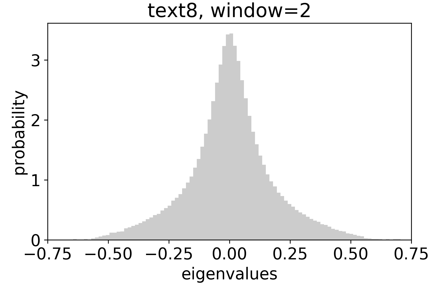
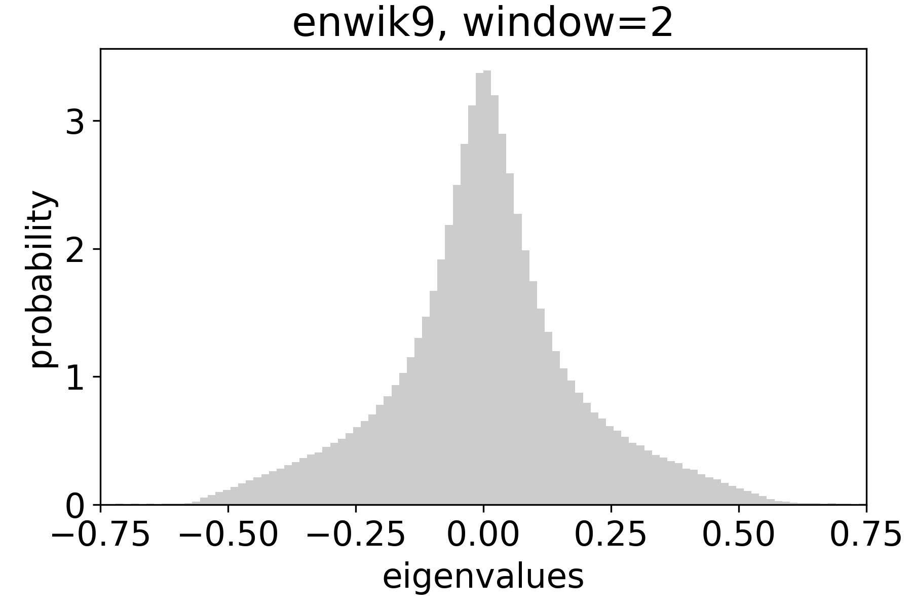
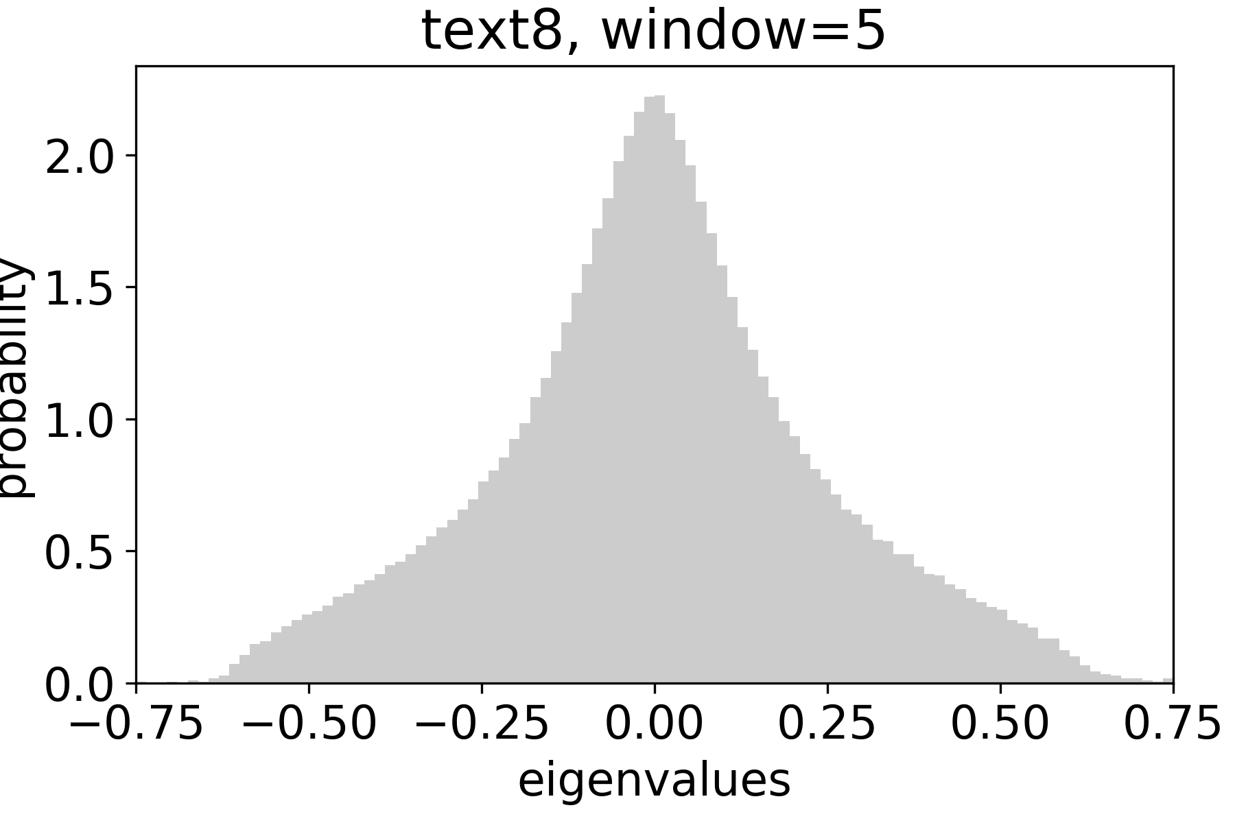
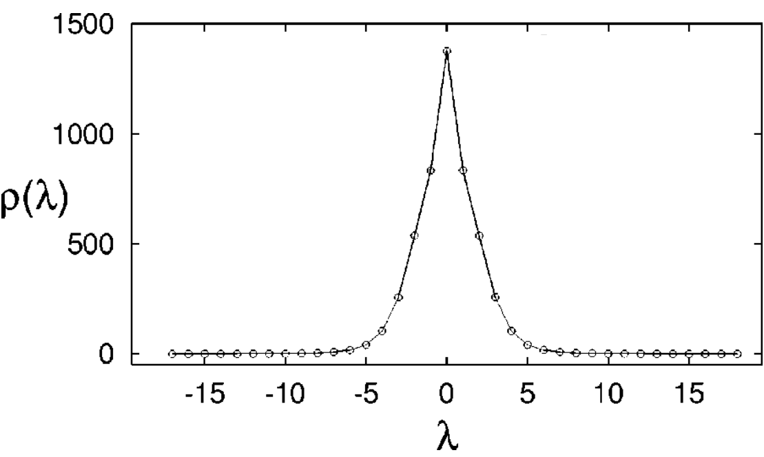
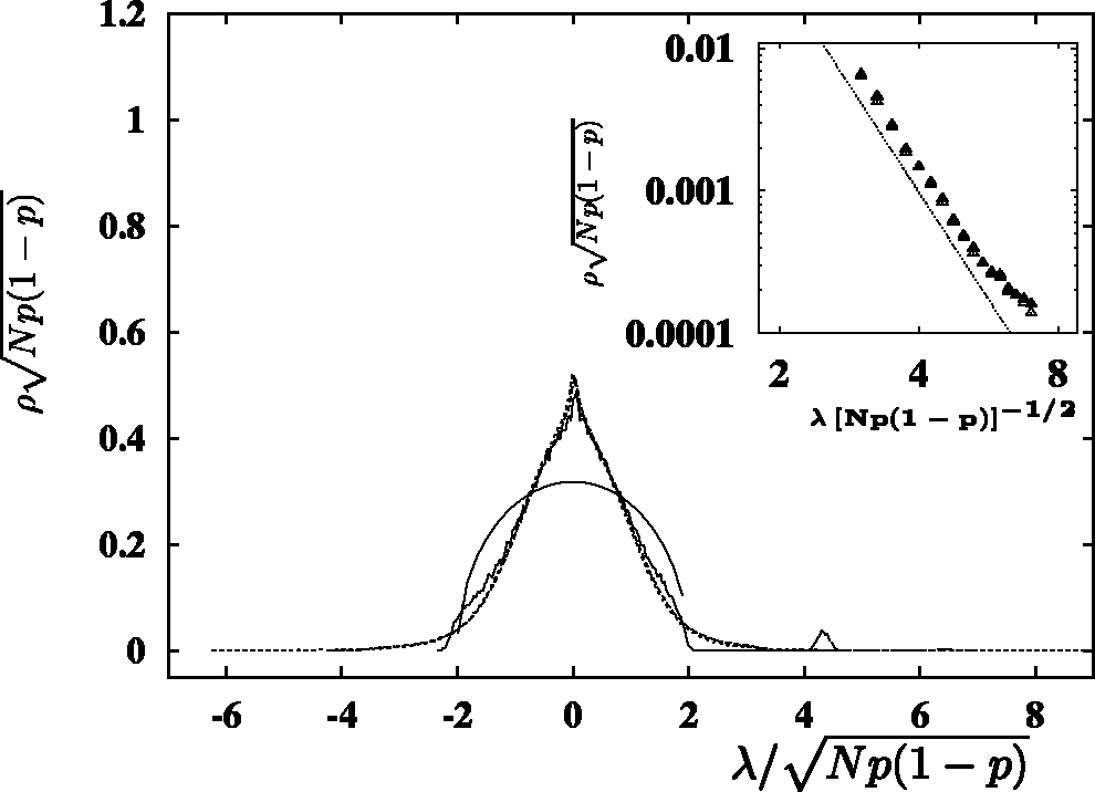
Figure 2: Spectral distribution of the $\sigma$SPMI-induced graphs (left and middle columns), and of scale-free random graphs with strong clustering property (right top: Goh et al. (2001), right bottom: Farkas et al. (2001)). When generating several random graphs from the same $\sigma$SPMI matrix, their eigenvalue distributions are visually indistinguishable, thus we display the results of one run per each matrix.

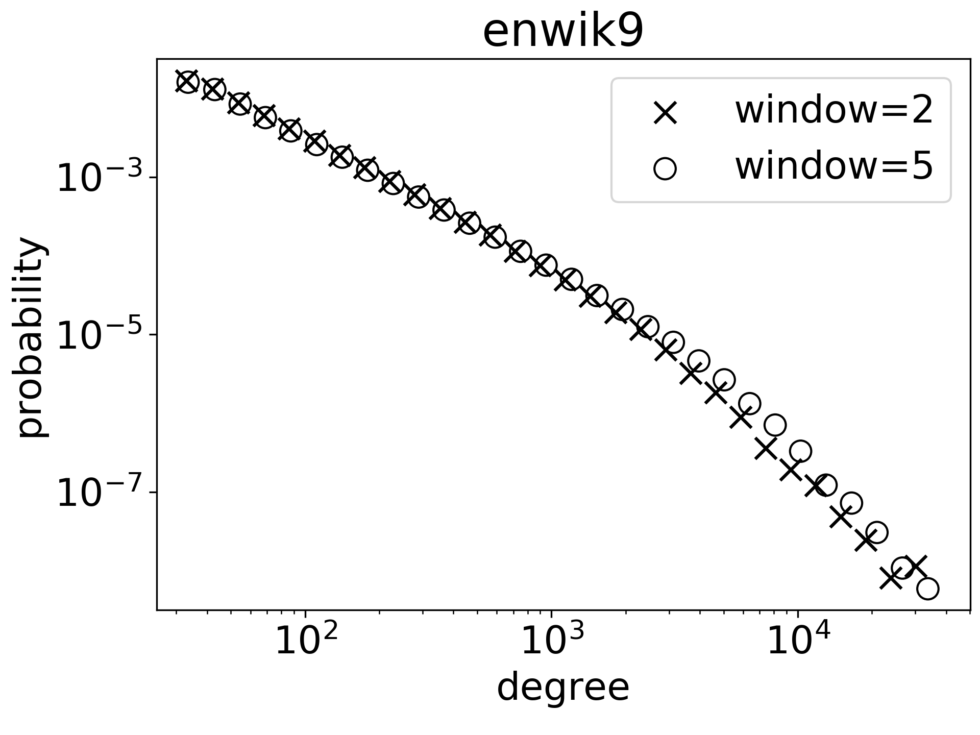
Figure 3: Degree distributions of the $\sigma$SPMI-induced graphs. The axes are on logarithmic scales.

Table 2: Clustering coefficients of the $\sigma$SPMI-induced graphs. For each corpus–window combination we generate ten graphs and report 95% confidence intervals across these ten runs.

	text8		enwik9
	window $=2$	window $=5$	window $=2$	window $=5$
$C$	$.1341\pm.0006$	$.1477\pm.0005$	$.1638\pm.0006$	$.1798\pm.0004$
$\bar{k}/n$	$.0014\pm.0000$	$.0030\pm.0000$	$.0006\pm.0000$	$.0012\pm.0000$

3 $\sigma$SPMI and Complex Networks

$\sigma$SPMI matrix has the following property: its entries $\sigma\text{SPMI}_{ij}\in[0,1)$ can be treated as connection probabilities for generating a random graph. As usually, by a graph $\mathcal{G}$ we mean a set of vertices $\mathcal{V}$ and a set of edges $\mathcal{E}\subset\mathcal{V}\times\mathcal{V}$. It is convenient to represent graph edges by its adjacency matrix $(e_{ij})$, in which $e_{ij}=1$ for $(i,j)\in\mathcal{E}$, and $e_{ij}=0$ otherwise. The graph with $\mathcal{V}:=\mathcal{W}$ and $e_{ij}\sim\text{Bernoulli}(\sigma\mathrm{SPMI}_{ij})$ will be referred to as $\sigma$SPMI-induced Graph.

3.1 Spectrum of the $\sigma$SPMI-induced Graph

First of all, we look at the spectral properties of the $\sigma$SPMI-induced Graphs. For this, we extract SPMI matrices from the text8 and enwik9 datasets using the hyperwords tool of Levy et al. (2015). We use the default settings for all hyperparameters, except the word frequency threshold and context window size. We ignored words that appeared less than 100 times and 250 times in text8 and enwik9 correspondingly, resulting in vocabularies of 11,815 and 21,104 correspondingly. We additionally experiment with the context window size 5, which by default is set to 2. We generate random graphs from the $\sigma$SPMI matrices and compute their eigenvalues using the TensorFlow library (Abadi et al., 2016), and the above-mentioned threshold of 250 for enwik9 was chosen to fit the GPU memory (11GB, RTX 2080 Ti). The eigenvalue distributions are provided in Figure 2.

The distributions seem to be symmetric, however, the shapes of distributions are far from resembling the Wigner semicircle law $x\mapsto\frac{1}{2\pi}\sqrt{4-x^{2}}$, which is the limiting distribution for the eigenvalues of many random symmetric matrices with i.i.d. entries (Wigner, 1955, 1958). This means that the entries of the $\sigma$SPMI-induced graph’s adjacency matrix are dependent, otherwise we would observe approximately semicircle distributions for its eigenvalues. We observe some similarity between the spectral distributions of the $\sigma$SPMI-induced graphs and of the so-called complex networks which arise in physics and network science (Figure 2).

Notice that the connection between human language structure and complex networks was observed previously by Cancho and Solé (2001). A thorough review on approaching human language with complex networks was given by Cong and Liu (2014). In the following subsection we will specify precisely what we mean by a complex network.

3.2 Clustering and Degree Distribution of the $\sigma$SPMI-induced Graph

We will use two statistical properties of a graph – degree distribution and clustering coefficient. The degree of a given vertex $i$ is the number of edges that connects it with other vertices, i.e. $\deg(i)=\sum_{j\in\mathcal{V}}e_{ij}$. The clustering coefficient measures the average fraction of pairs of neighbors of a vertex that are also neighbors of each other. The precise definition is as follows.

Let us indicate by $\mathcal{G}_{i}=\{j\in\mathcal{V}\mid e_{ij}=1\}$ the set of nearest neighbors of a vertex $i$. By setting $l_{i}=\sum_{j\in\mathcal{V}}e_{ij}\left[\sum_{k\in\mathcal{G}_{i};\ j<k}e_{jk}\right],$ we define the local clustering coefficient as $C(i)=\frac{l_{i}}{{|\mathcal{G}_{i}|\choose 2}}$, and the clustering coefficient as the average over $\mathcal{V}$: $C=\frac{1}{n}\sum_{i\in\mathcal{V}}C(i)$.

Let $\bar{k}$ be the average degree per vertex, i.e. $\bar{k}=\frac{1}{n}\sum_{j\in\mathcal{V}}e_{ij}$. For random binomial graphs, i.e. graphs with edges $e_{ij}\,\,{\stackrel{{\scriptstyle\text{iid}}}{{\sim}}}\,\,\mathrm{Bernoulli}(p)$, it is well known (Erdős and Rényi, 1960) that $C\approx\frac{\bar{k}}{n}$ and $\deg(i)\,\,\sim\,\,\mathrm{Binomial}(n-1,p)$. A complex network is a graph, for which $C\gg\frac{\bar{k}}{n}$ and $p(\deg(i)=k)\propto\frac{1}{k^{\gamma}}$, where $\gamma$ is some constant (Dorogovtsev, 2010). The latter property is referred to as scale-free (or power-law) degree distribution.

We constructed $\sigma$SPMI-induced Graphs from the text8 and enwik9 datasets using context windows of sizes 2 and 5 and ignoring words that appeared less than 5 times, and computed their clustering coefficients (Table 2) as well as degree distributions (Figure 3) using the NetworKit tool (Staudt et al., 2016). NetworKit uses the algorithm of Schank and Wagner (2005) to compute the clustering coefficient. As we see, the $\sigma$SPMI-induced graphs are complex networks, and this brings us to the hyperbolic spaces.

4 Complex Networks and Hyperbolic Geometry

Complex networks are “dual” to hyperbolic spaces as was shown by Krioukov et al. (2010). They showed that any complex network, as defined in Section 3, has an effective hyperbolic geometry underneath. Apart from this, they also showed that any hyperbolic geometry implies a complex network: they placed randomly $n$ points (nodes) into a hyperbolic disk of radius $R$, and used $p_{ij}:=\sigma\left(c[R-x_{ij}]\right)$ as connection probability for connecting nodes $i$ and $j$, where $x_{ij}$ is the hyperbolic distance between $i$ and $j$, and $c$ is a constant. An example of such random graph is shown in Figure 5.

Figure 4: Rand. hyperbolic graph.

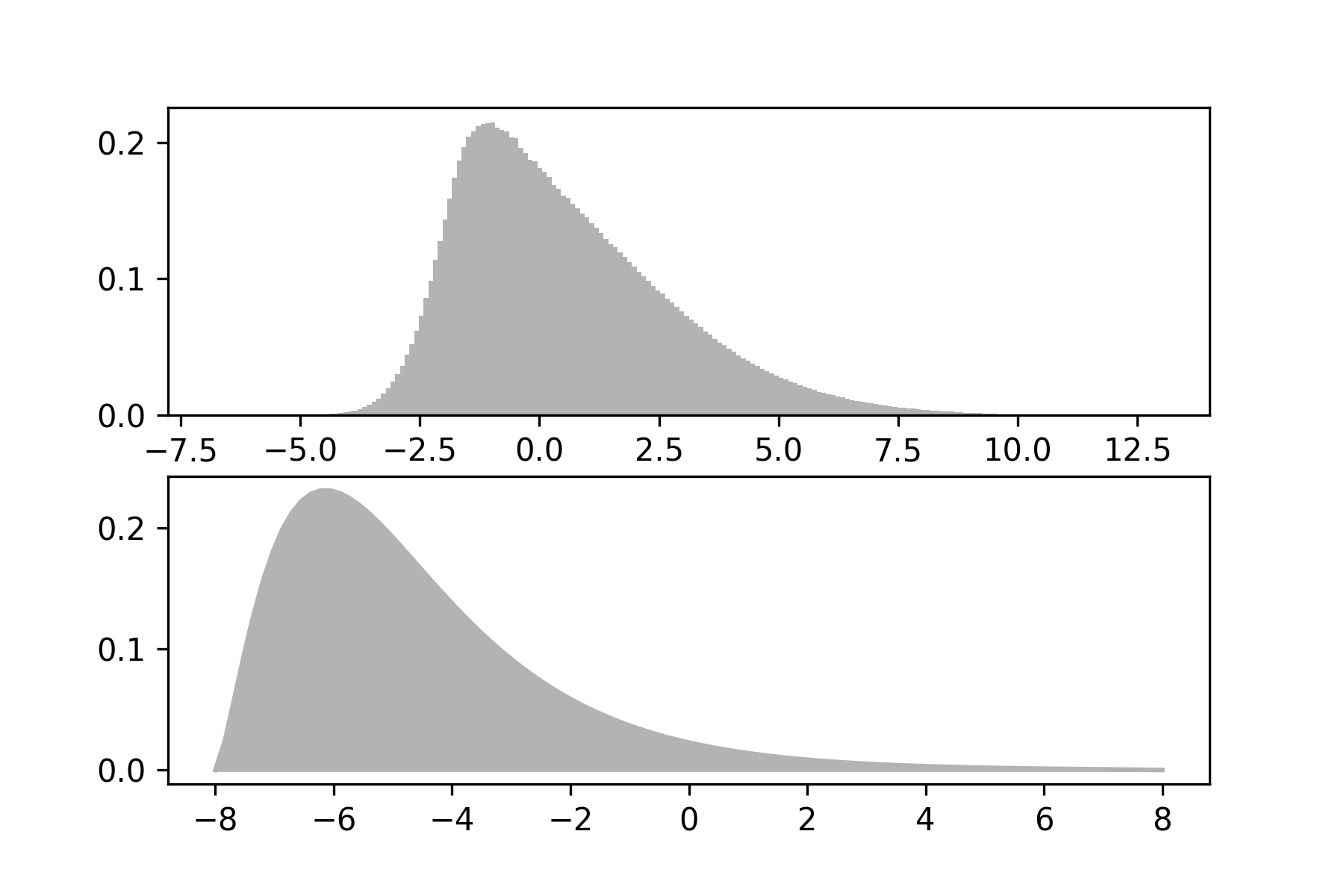
Figure 5: SPMI values distr’n (top) vs $R-X$.

Krioukov et al. (2010) showed that the resulting graph is a complex network. They establish connections between the clustering coefficient $C$ and the power-law exponent $\gamma$ of a complex network and the curvature of a hyperbolic space.

Comparing the construction of Krioukov et al. (2010) to the way we generate a random graph from the $\sigma$SPMI matrix, and taking into account that both methods produce similar structures (complex networks), we conclude that the distribution of the SPMI values should be similar to the distribution of $R-x_{ij}$, i.e. $\text{PMI}_{ij}-\log k\sim R-x_{ij}$. To verify this claim we compare the distribution of SPMI values with the p.d.f. of a random variable $R-X$, where $X$ is a hyperbolic distance between two random points on the hyperbolic disk (the exact form of this p.d.f. is given in the Appendix 0.A). $R$ was chosen according to the formula $R=2\ln[8n/(\pi\bar{k})]$ (Krioukov et al., 2010), where $\bar{k}$ is the average degree of the $\sigma$SPMI-induced Graph. The results are shown in Figure 5. As we can see, the two distributions are indeed similar and the main difference is in the shift—distribution of $R-X$ is shifted to the left compared to the distribution of the SPMI values. This allows us reinterpreting the pointwise mutual information as the negative of hyperbolic distance (up to scaling and shifting).

5 Conclusion

It is noteworthy that the seemingly fragmented sections of scientific knowledge can be closely interconnected. In this paper, we have established a chain of connections between word embeddings and hyperbolic geometry, and the key link in this chain is the Squashed Shifted PMI matrix. Claiming that hyperbolicity underlies word vectors is not novel (Nickel and Kiela, 2017; Tifrea et al., 2018). However, this work is the first attempt to justify the connection between hyperbolic geometry and the word embeddings. In the course of our work, we discovered novel objects—Nonsigmoid SGNS and Squashed Shifted PMI matrix—which can be investigated separately in the future.

Appendix 0.A Auxiliary Results

Proposition 1

Let $X$ be a distance between two points that were randomly uniformly placed in the hyperbolic disk of radius $R$. The probability distribution function of $X$ is given by

$$f_{X}(x)=\int_{0}^{R}\int_{0}^{R}\frac{\sinh(x)}{\pi\sqrt{1-A(r_{1},r_{2},x)}\sinh(r_{1})\sinh(r_{2})}\rho(r_{1})\rho(r_{2})dr_{1}dr_{2},$$ (7)

where $A(r_{1},r_{2},x)=\frac{\cosh(r_{1})\cosh(r_{2})-\cosh(x)}{\sinh(r_{1})\sinh(r_{2})}$, and $\rho(r)=\frac{\sinh r}{\cosh R-1}$.

The proof is by direct calculation and is omitted due to page limit.

References

- Abadi et al. (2016) Abadi, M., Barham, P., Chen, J., Chen, Z., Davis, A., Dean, J., Devin, M., Ghemawat, S., Irving, G., Isard, M., et al.: Tensorflow: A system for large-scale machine learning. In: Proceedings of OSDI. pp. 265–283 (2016)
- Allen et al. (2019) Allen, C., Balazevic, I., Hospedales, T.: What the vec? towards probabilistically grounded embeddings. In: Advances in Neural Information Processing Systems. pp. 7465–7475 (2019)
- Allen and Hospedales (2019) Allen, C., Hospedales, T.: Analogies explained: Towards understanding word embeddings. In: International Conference on Machine Learning. pp. 223–231 (2019)
- Arora et al. (2016) Arora, S., Li, Y., Liang, Y., Ma, T., Risteski, A.: A latent variable model approach to pmi-based word embeddings. Transactions of the Association for Computational Linguistics 4, 385–399 (2016)
- Assylbekov and Takhanov (2019) Assylbekov, Z., Takhanov, R.: Context vectors are reflections of word vectors in half the dimensions. Journal of Artificial Intelligence Research 66, 225–242 (2019)
- Bruni et al. (2012) Bruni, E., Boleda, G., Baroni, M., Tran, N.K.: Distributional semantics in technicolor. In: Proceedings of ACL. pp. 136–145. Association for Computational Linguistics (2012)
- Cancho and Solé (2001) Cancho, R.F.I., Solé, R.V.: The small world of human language. Proceedings of the Royal Society of London. Series B: Biological Sciences 268(1482), 2261–2265 (2001)
- Cong and Liu (2014) Cong, J., Liu, H.: Approaching human language with complex networks. Physics of life reviews 11(4), 598–618 (2014)
- Devlin et al. (2019) Devlin, J., Chang, M.W., Lee, K., Toutanova, K.: Bert: Pre-training of deep bidirectional transformers for language understanding. In: Proceedings of NAACL-HLT. pp. 4171–4186 (2019)
- Dorogovtsev (2010) Dorogovtsev, S.: Lectures on Complex Networks. Oxford University Press, Inc., USA (2010)
- Eckart and Young (1936) Eckart, C., Young, G.: The approximation of one matrix by another of lower rank. Psychometrika 1(3), 211–218 (1936)
- Erdős and Rényi (1960) Erdős, P., Rényi, A.: On the evolution of random graphs. Publ. Math. Inst. Hung. Acad. Sci 5(1), 17–60 (1960)
- Ethayarajh et al. (2019) Ethayarajh, K., Duvenaud, D., Hirst, G.: Towards understanding linear word analogies. In: Proceedings of the 57th Annual Meeting of the Association for Computational Linguistics. pp. 3253–3262 (2019)
- Farkas et al. (2001) Farkas, I.J., Derényi, I., Barabási, A.L., Vicsek, T.: Spectra of “real-world” graphs: Beyond the semicircle law. Physical Review E 64(2), 026704 (2001)
- Finkelstein et al. (2002) Finkelstein, L., Gabrilovich, E., Matias, Y., Rivlin, E., Solan, Z., Wolfman, G., Ruppin, E.: Placing search in context: The concept revisited. ACM Transactions on information systems 20(1), 116–131 (2002)
- Gittens et al. (2017) Gittens, A., Achlioptas, D., Mahoney, M.W.: Skip-gram- zipf+ uniform= vector additivity. In: Proceedings of the 55th Annual Meeting of the Association for Computational Linguistics (Volume 1: Long Papers). pp. 69–76 (2017)
- Goh et al. (2001) Goh, K.I., Kahng, B., Kim, D.: Spectra and eigenvectors of scale-free networks. Physical Review E 64(5), 051903 (2001)
- Hashimoto et al. (2016) Hashimoto, T.B., Alvarez-Melis, D., Jaakkola, T.S.: Word embeddings as metric recovery in semantic spaces. Transactions of the Association for Computational Linguistics 4, 273–286 (2016)
- Krioukov et al. (2010) Krioukov, D., Papadopoulos, F., Kitsak, M., Vahdat, A., Boguná, M.: Hyperbolic geometry of complex networks. Physical Review E 82(3), 036106 (2010)
- Levy and Goldberg (2014a) Levy, O., Goldberg, Y.: Linguistic regularities in sparse and explicit word representations. In: Proceedings of CoNLL. pp. 171–180 (2014a)
- Levy and Goldberg (2014b) Levy, O., Goldberg, Y.: Neural word embedding as implicit matrix factorization. In: Proceedings of NeurIPS. pp. 2177–2185 (2014b)
- Levy et al. (2015) Levy, O., Goldberg, Y., Dagan, I.: Improving distributional similarity with lessons learned from word embeddings. Transactions of the Association for Computational Linguistics 3, 211–225 (2015)
- Luong et al. (2013) Luong, T., Socher, R., Manning, C.: Better word representations with recursive neural networks for morphology. In: Proceedings of CoNLL. pp. 104–113 (2013)
- McCann et al. (2017) McCann, B., Bradbury, J., Xiong, C., Socher, R.: Learned in translation: Contextualized word vectors. In: Advances in Neural Information Processing Systems. pp. 6294–6305 (2017)
- Mikolov et al. (2013a) Mikolov, T., Chen, K., Corrado, G., Dean, J.: Efficient estimation of word representations in vector space. arXiv preprint arXiv:1301.3781 (2013a)
- Mikolov et al. (2013b) Mikolov, T., Sutskever, I., Chen, K., Corrado, G.S., Dean, J.: Distributed representations of words and phrases and their compositionality. In: Advances in neural information processing systems. pp. 3111–3119 (2013b)
- Mikolov et al. (2013c) Mikolov, T., Yih, W.t., Zweig, G.: Linguistic regularities in continuous space word representations. In: Proceedings of the 2013 Conference of the North American Chapter of the Association for Computational Linguistics: Human Language Technologies. pp. 746–751 (2013c)
- Nickel and Kiela (2017) Nickel, M., Kiela, D.: Poincaré embeddings for learning hierarchical representations. In: Advances in neural information processing systems. pp. 6338–6347 (2017)
- Pedregosa et al. (2011) Pedregosa, F., Varoquaux, G., Gramfort, A., Michel, V., Thirion, B., Grisel, O., Blondel, M., Prettenhofer, P., Weiss, R., Dubourg, V., Vanderplas, J., Passos, A., Cournapeau, D., Brucher, M., Perrot, M., Duchesnay, E.: Scikit-learn: Machine learning in Python. Journal of Machine Learning Research 12, 2825–2830 (2011)
- Pennington et al. (2014) Pennington, J., Socher, R., Manning, C.: Glove: Global vectors for word representation. In: Proceedings of EMNLP. pp. 1532–1543 (2014)
- Peters et al. (2018) Peters, M.E., Neumann, M., Iyyer, M., Gardner, M., Clark, C., Lee, K., Zettlemoyer, L.: Deep contextualized word representations. In: Proceedings of NAACL-HLT. pp. 2227–2237 (2018)
- Radinsky et al. (2011) Radinsky, K., Agichtein, E., Gabrilovich, E., Markovitch, S.: A word at a time: computing word relatedness using temporal semantic analysis. In: Proceedings of the 20th international conference on World wide web. pp. 337–346. ACM (2011)
- Řehůřek and Sojka (2010) Řehůřek, R., Sojka, P.: Software Framework for Topic Modelling with Large Corpora. In: Proceedings of the LREC 2010 Workshop on New Challenges for NLP Frameworks. pp. 45–50. ELRA, Valletta, Malta (May 2010), http://is.muni.cz/publication/884893/en
- Reif et al. (2019) Reif, E., Yuan, A., Wattenberg, M., Viegas, F.B., Coenen, A., Pearce, A., Kim, B.: Visualizing and measuring the geometry of bert. In: Advances in Neural Information Processing Systems. pp. 8592–8600 (2019)
- Schank and Wagner (2005) Schank, T., Wagner, D.: Approximating clustering coefficient and transitivity. Journal of Graph Algorithms and Applications 9(2), 265–275 (2005)
- Staudt et al. (2016) Staudt, C.L., Sazonovs, A., Meyerhenke, H.: Networkit: A tool suite for large-scale complex network analysis. Network Science 4(4), 508–530 (2016)
- Tian et al. (2017) Tian, R., Okazaki, N., Inui, K.: The mechanism of additive composition. Machine Learning 106(7), 1083–1130 (2017)
- Tifrea et al. (2018) Tifrea, A., Bécigneul, G., Ganea, O.E.: Poincaré glove: Hyperbolic word embeddings. arXiv preprint arXiv:1810.06546 (2018)
- Wigner (1955) Wigner, E.P.: Characteristic vectors of bordered matrices with infinite dimensions. Annals of Mathematics pp. 548–564 (1955)
- Wigner (1958) Wigner, E.P.: On the distribution of the roots of certain symmetric matrices. Annals of Mathematics pp. 325–327 (1958)
- Zobnin and Elistratova (2019) Zobnin, A., Elistratova, E.: Learning word embeddings without context vectors. In: Proceedings of the 4th Workshop on Representation Learning for NLP (RepL4NLP-2019). pp. 244–249 (2019)