Finite element approximation of a system coupling curve evolution with prescribed normal contact to a fixed boundary to reaction-diffusion on the curve

Abstract

We consider a finite element approximation for a system consisting of the evolution of a curve evolving by forced curve shortening flow coupled to a reaction-diffusion equation on the evolving curve. The curve evolves inside a given domain $\Omega\subset\mathbb{R}^{2}$ and meets $\partial\Omega$ orthogonally. The scheme for the coupled system is based on the schemes derived in BDS17 and DE98 . We present numerical experiments and show the experimental order of convergence of the approximation.

1 Introduction

We consider a curve $\Gamma(t)$ evolving by forced curve shortening flow inside a given bounded domain $\Omega\subset\mathbb{R}^{2}$, with the forcing being a function of the solution, $w\text{ : }\Gamma(t)\rightarrow\mathbb{R}$, of a reaction-diffusion equation that holds on $\Gamma(t)$, such that

$$v =\kappa+f(w) \text{ on }\Gamma(t),\text{ }t\in(0,T],$$ (1)

$$\partial^{\bullet}_{t}w =w_{ss}+\kappa\,v\,w+g(v,w) \text{ on }\Gamma(t),\text{ }t\in(0,T],$$ (2)

subject to the initial data $\Gamma(0)=\Gamma_{0}$ and $w(\cdot,0)=w_{0}\text{ on }\Gamma_{0}$.

Here $v$ and $\kappa$ respectively denote the normal velocity and mean curvature of $\Gamma(t)$, corresponding to the choice $\vec{\vec{n}}$ of a unit normal, $s$ is the arclength parameter on $\Gamma(t)$ and $\partial^{\bullet}_{t}w:=w_{t}+v\frac{\partial w}{\partial\vec{n}}$ denotes the material derivative of $w$. In addition we impose that the curve meets the boundary $\partial\Omega$ orthogonally. To this end we assume that $\partial\Omega$ is given by a smooth function $F$ such that

$$\partial\Omega=\{p\in\mathbb{R}^{2}:F(p)=0\}~{}~{}\text{and}~{}~{}|\nabla F(p)|=1~{}~{}\forall~{}p\in\partial\Omega.$$

Coupling the parametrisation of (1), (2) that is presented in BDS17 for the setting in which $\Gamma(t)$ is a closed curve, with the formulation of (1) presented in DE98 for the setting in which $\Gamma(t)$ meets the boundary $\partial\Omega$ orthogonally, yields the following system:

$$\alpha\vec{x}_{t}+(1-\alpha)(\vec{x}_{t}\cdot\vec{\vec{n}})\,\vec{\vec{n}}=\frac{\vec{x}_{\rho\rho}}{|\vec{x}_{\rho}|^{2}}+f(w)\,\vec{\vec{n}},\qquad\qquad\quad\,\,\text{ for }(\rho,t)\in\mathbb{I}\times(0,T)$$ (3)

$$w_{t}-(\vec{x}_{t}\cdot\vec{\tau})\,\frac{1}{|\vec{x}_{\rho}|}\,w_{\rho}-\frac{1}{|\vec{x}_{\rho}|}\left(\frac{w_{\rho}}{|\vec{x}_{\rho}|}\right)_{\rho}-\kappa\,v\,w=g(v,w),\text{ for }(\rho,t)\in\mathbb{I}\times(0,T)$$ (4)

$$\vec{x}(\rho,0)=\vec{x}_{0}(\rho),~{}~{}~{}~{}w(\rho,0)=w_{0}(\rho)\qquad\qquad\qquad\qquad\,\,\,\,\,\text{ for }\rho\in\mathbb{I}$$ (5)

$$w(\rho,t)=w_{b},\qquad\qquad\qquad\qquad\qquad\qquad\qquad\quad\text{ for }(\rho,t)\in\{0,1\}\times[0,T]\,$$ (6)

$$F(\vec{x}(\rho,t))=0,\qquad\qquad\qquad\qquad\qquad\qquad\qquad\,\,\,\text{ for }(\rho,t)\in\{0,1\}\times[0,T]$$ (7)

$$(\vec{x}_{\rho}(\rho,t)\cdot\nabla^{\perp}F(\vec{x}(\rho,t))=0,\qquad\qquad\qquad\qquad\,\,\,\,\,\,\text{ for }(\rho,t)\in\{0,1\}\times[0,T].$$ (8)

Here $\alpha\in(0,1]$, $\mathbb{I}:=(0,1)$, $\vec{x}(\cdot,t):[0,1]\rightarrow\mathbb{R}^{2}$, $w(\rho,t):=w(\vec{x}(\rho,t),t)$, $(\rho,t)\in[0,1]\times[0,T]$, and the unit tangent and unit normal to $\Gamma(t)$ are respectively given by $\vec{\tau}=\vec{x}_{s}=\frac{\vec{x}_{\rho}}{|\vec{x}_{\rho}|}$ and $\vec{\vec{n}}=\vec{\tau}^{\perp}$ where $(\cdot)^{\perp}$ denotes counter-clockwise rotation by $\frac{\pi}{2}$.

The formulation of curve shortening flow in the form of (3) for a closed curve in $\mathbb{R}^{2}$ was presented and analysed in EF16 , where the DeTurck trick is used in coupling the motion of the curve to the harmonic map heat flow, with the parameter $\alpha\in(0,1]$ being such that $1/\alpha$ corresponds to the diffusion coefficient in the harmonic map heat flow. Setting $\alpha\in(0,1]$ introduces a tangential part in the velocity which, at the numerical level, gives rise to a good distribution of the mesh points along the curve. Setting $\alpha=1$ one recovers the formulation introduced and analysed in DD95 , while formally setting $\alpha=0$ yields the approach introduced in BGN11 . In DES01 the authors derive finite element approximations of a simplified version of the parametric coupled system (3)-(8), and two related models. In particular, the evolution law for the parametric system derived in DES01 , can be obtained from (3) by setting $\alpha=1$, $F(x,y)=|x|-1$, and considering a slightly different formulation of the reaction-diffusion equation (4). In BDS17 the authors prove optimal error bounds for a fully discrete finite element approximation of the coupled system (3)-(5) for the case where $\Gamma(t)$ is a closed curve in $\mathbb{R}^{2}$. While in PS15 optimal error bounds are presented for a semi-discrete finite element approximation of an alternative formulation, which is introduced and analysed in D94 , of the coupled system (3)-(5), for the case where $\Gamma(t)$ is a closed curve in $\mathbb{R}^{2}$. Setting $\alpha=1$ and $f(w)=0$ in (3) and coupling the resulting equation to (7), (8) gives rise to the model presented and analysed in DE98 , in which optimal order error bounds for a semi-discrete finite element approximation of curve shortening flow with a prescribed normal contact to a fixed boundary are presented. In BGN07b the authors propose parametric finite element approximations of combined second and fourth order geometric evolution equations for curves that are connected via triple or quadruple junctions or that intersect external boundaries.

2 Weak formulation and finite element approximation

For a weak formulation of (3) we multiply it by $|\vec{x}_{\rho}|^{2}\vec{\xi}$, where $\vec{\xi}\in[H^{1}(\mathbb{I})]^{2}$ is a test function, integrate in space, use integration by parts and (8) to obtain

$$\left(|\vec{x}_{\rho}|^{2}\left[\alpha\,\vec{x}_{t}+(1-\alpha)(\vec{x}_{t}\cdot\vec{\vec{n}})\,\vec{\vec{n}}\,\right],\vec{\xi}\right)+\left(\vec{x}_{\rho},\vec{\xi}_{\rho}\right)$$

$$\quad=\left[(\vec{x}_{\rho}\cdot\nabla F(\vec{x}))(\vec{\xi}\cdot\nabla F(\vec{x}))\right]_{0}^{1}+\left(|\vec{x}_{\rho}|^{2}f(w)\,\vec{\vec{n}},\vec{\xi}\right)\qquad\forall\,\vec{\xi}\in[H^{1}(\mathbb{I})]^{2},$$ (9)

where $(\cdot,\cdot)$ denotes the standard $L^{2}(\mathbb{I})$ inner product. For a weak formulation of (4) we multiply it by $|\vec{x}_{\rho}|\,\eta$, where $\eta\in H_{0}^{1}(\mathbb{I})$ is a time-independent test function, integrate in space, use integration by parts and note that $\vec{\tau}_{\rho}=\kappa\,\vec{\vec{n}}\,|\vec{x}_{\rho}|$ to obtain

$$\frac{d}{dt}\left(|\vec{x}_{\rho}|\,w,\eta\right)+\left(\psi\,w,\eta_{\rho}\right)+\left(\frac{w_{\rho}}{|\vec{x}_{\rho}|},\eta_{\rho}\right)=\left(|\vec{x}_{\rho}|\,g(v,w),\eta\right)\quad\forall\,\eta\in H_{0}^{1}(\mathbb{I}).$$ (10)

Here $\psi$ is the tangential velocity of $\Gamma(t)$, such that the normal and tangential velocities of $\Gamma(t)$ are given by $v=\vec{x}_{t}\cdot\vec{\vec{n}}$ and $\psi=\vec{x}_{t}\cdot\vec{\tau}$. We now introduce a finite element approximation of (2), (10). We first let $0=t_{0}<t_{1}<\cdots<t_{N-1}<t_{N}=T$ be a partition of $[0,T]$ with $\Delta t_{n}:=t_{n}-t_{n-1}$. Next we partition the interval $\mathbb{I}$ such that $\mathbb{I}=\cup_{j=1}^{J}\overline{\sigma_{j}}$, where $\sigma_{j}=(\rho_{j-1},\rho_{j})$, with $h_{j}=\rho_{j}-\rho_{j-1}$. We set

$$V^{h} :=\{\chi\in C(\mathbb{I})\text{ : }\chi_{|_{\sigma_{j}}}\text{ is affine, }j=1,\dots,J\}\subset H^{1}(\mathbb{I})$$

$$V_{0}^{h} :=\{\chi\in V^{h}\text{ : }\chi(\rho_{j})=0,\text{ for }j\in\{0,J\}\}$$

and denote the standard Lagrange interpolation operator by $I^{h}\text{ : }C(\mathbb{I})\rightarrow V^{h}$, where $(I^{h}\eta)(\rho_{j})=\eta(\rho_{j})$, for $j=1,\dots,J$. We define the discrete inner product $(\eta_{1},\eta_{2})^{h}$ by

$$\left(\eta_{1},\eta_{2}\right)^{h} :=\sum_{j=1}^{J}\int_{\sigma_{j}}I^{h}_{j}(\eta_{1}\,\eta_{2})\,\;{\rm d}\rho,$$

where $I^{h}_{j}=I^{h}_{|_{\sigma_{j}}}$ is the local interpolation operator. Our finite element approximation of (2), (10) then takes the form:

Given $(\vec{X}^{n-1},W^{n-1}-w_{b})\in[V^{h}]^{2}\times V_{0}^{h}$, find $(\vec{X}^{n},W^{n}-w_{b})\in[V^{h}]^{2}\times V_{0}^{h}$ such that for all $(\vec{\xi}^{h},\eta^{h})\in[V^{h}]^{2}\times V_{0}^{h}$ we have

$$\SwapAboveDisplaySkip\left(|\vec{X}_{\rho}^{n-1}|^{2}\left[\alpha D_{t}\vec{X}^{n}+(1-\alpha)(D_{t}\vec{X}^{n}\cdot\vec{\mathcal{N}}^{n-1})\,\vec{\mathcal{N}}^{n-1}\right],\vec{\xi}^{h}\right)^{h}+\left(\vec{X}^{n}_{\rho},\vec{\xi}^{h}_{\rho}\right)\hskip 28.45274pt$$

$$=\left[(\vec{X}^{n}_{\rho}\cdot\nabla F(\vec{X}^{n}))(\vec{\xi}^{h}\cdot\nabla F(\vec{X}^{n}))\right]^{1}_{0}+\left(|\vec{X}_{\rho}^{n-1}|^{2}f(W^{n-1})\,\vec{\mathcal{N}}^{n-1},\vec{\xi}^{h}\right)^{h}$$ (11)

$$D_{t}\left[\left(|\vec{X}_{\rho}^{n}|\,W^{n},\eta^{h}\right)^{h}\right]+\left(\frac{W^{n}_{\rho}}{|\vec{X}_{\rho}^{n}|},\eta^{h}_{\rho}\right)+\left(\Psi^{n}\,W^{n},\eta^{h}_{\rho}\right)^{h}\hskip 79.66771pt$$

$$=\left(|\vec{X}_{\rho}^{n}|\,g(V^{n},W^{n-1}),\eta^{h}\right)^{h}~{}~{}~{}~{}~{}~{}$$ (12)

with the additional boundary constraint

$$F(\vec{X}^{n}_{0})=F(\vec{X}^{n}_{J})=0.$$ (13)

Here and in what follows we set $D_{t}(a^{n}):=(a^{n}-a^{n-1})/\Delta t_{n}$ and on $\sigma_{j}$, $j=1,\cdots,J$ we set $\vec{\mathcal{T}}^{n}=\frac{\vec{X}^{n}_{\rho}}{|\vec{X}_{\rho}^{n}|}$ , $\vec{\mathcal{N}}^{n}=(\vec{\mathcal{T}}^{n})^{\perp}$, $\Psi^{n}=D_{t}\vec{X}^{n}\cdot\vec{\mathcal{T}}^{n}$ and $V^{n}=D_{t}\vec{X}^{n}\cdot\vec{\mathcal{N}}^{n}$.

Remark 1

In DE98 , rather than use the nonlinear scheme presented above to approximate (3), (7), (8), the authors present a linear scheme in which (7) is not necessarily satisfied but is instead approximated through the relation $0=\frac{d}{dt}F(\vec{x})=\vec{x}_{t}\cdot\nabla F(\vec{x})$.

3 Numerical results

3.1 Solution of the discrete system (11), (13)

We solve the resulting system of nonlinear algebraic equations arising at each time level from the approximation (11), (13), with $\vec{\xi}^{h}=\chi_{j}$, $j=1,\dots,J-1$, $\vec{\xi}^{h}=\nabla^{\perp}F(\vec{X}^{n})\chi_{0}$ and $\vec{\xi}^{h}=\nabla^{\perp}F(\vec{X}^{n})\chi_{J}$, using the following Newton scheme, where for ease of presentation we set $\alpha=1$ and $f(w)=0$:

Given $\vec{X}^{n,i-1}$, with $\vec{X}^{n,0}=\vec{X}^{n-1}$, we set $\vec{X}^{n,i}:=\vec{X}^{n,i-1}+\vec{\delta}^{i}$ such that for $j=1,\dots,J-1$, $\vec{\delta}^{i}$ solves

$$\frac{1}{2}\left(q_{j}^{n-1}+q_{j-1}^{n-1}\right)\frac{\vec{\delta}_{j}^{i}}{\Delta t_{n}}-\left(\vec{\delta}_{j-1}^{i}-2\vec{\delta}_{j}^{i}+\vec{\delta}_{j+1}^{i}\right)$$

$$\quad=-\frac{1}{2}\left(q_{j}^{n-1}+q_{j-1}^{n-1}\right)D_{t}(\vec{X}^{n,i-1}_{j})+\left(\vec{X}^{n,i-1}_{j-1}-2\vec{X}^{n,i-1}_{j}+\vec{X}^{n,i-1}_{j+1}\right),$$ (14a)

$$\frac{1}{2}\,{q^{n-1}_{0}}\left[\left(\frac{\vec{\delta}_{0}^{i}}{\Delta t_{n}}\cdot\nabla^{\perp}F(\vec{X}^{n,i-1}_{0})\right)+\left(D_{t}(\vec{X}^{n,i-1}_{0})\cdot D_{\perp}^{2}F(\vec{X}^{n,i-1}_{0})\,\vec{\delta}_{0}^{i}\right)\right]$$ (14b)

$$\quad-\left((\vec{\delta}_{1}^{i}-\vec{\delta}_{0}^{i})\cdot\nabla^{\perp}F(\vec{X}^{n,i-1}_{0})\right)-\left((\vec{X}^{n,i-1}_{1}-\vec{X}^{n,i-1}_{0})\cdot D_{\perp}^{2}F(\vec{X}^{n,i-1}_{0})\,\vec{\delta}_{0}^{i}\right)$$

$$\quad=-\frac{1}{2}\,q^{n-1}_{0}\left(D_{t}(\vec{X}^{n,i-1}_{0})\cdot\nabla^{\perp}F(\vec{X}^{n,i-1}_{0})\right)+\left((\vec{X}^{n,i-1}_{1}-\vec{X}^{n,i-1}_{0})\cdot\nabla^{\perp}F(\vec{X}^{n,i-1}_{0})\right),$$

$$\frac{1}{2}\,{q^{n-1}_{J-1}}\left[\left(\frac{\vec{\delta}_{J}^{i}}{\Delta t_{n}}\cdot\nabla^{\perp}F(\vec{X}^{n,i-1}_{J})\right)+\left(D_{t}(\vec{X}^{n,i-1}_{J})\cdot D_{\perp}^{2}F(\vec{X}^{n,i-1}_{J})\,\vec{\delta}_{J}^{i}\right)\right]$$ (14c)

$$\quad-\left((\vec{\delta}_{J-1}^{i}-\vec{\delta}_{J}^{i})\cdot\nabla^{\perp}F(\vec{X}^{n,i-1}_{J})\right)-\left((\vec{X}^{n,i-1}_{J-1}-\vec{X}^{n,i-1}_{J})\cdot D_{\perp}^{2}F(\vec{X}^{n,i-1}_{J})\,\vec{\delta}_{J}^{i}\right)$$

$$\quad=-\frac{1}{2}\,q^{n-1}_{J-1}\left(D_{t}(\vec{X}^{n,i-1}_{J})\cdot\nabla^{\perp}F(\vec{X}^{n,i-1}_{J})\right)+\left((\vec{X}^{n,i-1}_{J-1}-\vec{X}^{n,i-1}_{J})\cdot\nabla^{\perp}F(\vec{X}^{n,i-1}_{J})\right),$$

$$\left(\nabla F(\vec{X}^{n,i-1}_{0})\cdot\vec{\delta}^{i}_{0}\right)=-F(\vec{X}^{n,i-1}_{0})~{}~{}\text{and}~{}~{}\left(\nabla F(\vec{X}^{n,i-1}_{J})\cdot\vec{\delta}^{i}_{J}\right)=-F(\vec{X}^{n,i-1}_{J}),$$ (14d)

where $q_{j}^{n-1}=|\vec{X}^{n-1}_{j+1}-\vec{X}^{n-1}_{j}|^{2}$, $D^{2}_{\perp}=\left(\begin{matrix}-\partial^{2}_{xy}&-\partial^{2}_{yy}\\ \partial^{2}_{xx}&\partial^{2}_{xy}\end{matrix}\right)$, and in an abuse of notation we have redefined $D_{t}$ from the previous section such that $D_{t}(\vec{X}^{n,i-1}_{j}):=(\vec{X}^{n,i-1}_{j}-\vec{X}^{n-1}_{j})/\Delta t_{n}$. We adopt the stopping criteria $\max\limits_{j=0,J}|F(\vec{X}_{j}^{n,i})|\leq\tau$ for some predetermined tolerance, $\tau$.

3.2 Experimental order of convergence of (11), (13)

We investigate the experimental order of convergence of (11), (13) by monitoring the following errors:

$$\mathcal{E}_{1}:=\sup_{n=0,\dots,N}\|I^{h}(\vec{x}_{\rho}^{n})-\vec{X}_{\rho}^{n}\|_{[L^{2}(\mathbb{I})]^{2}}^{2},\quad\mathcal{E}_{2}:=\sum_{n=1}^{N}\Delta t_{n}\|D_{t}(I^{h}(\vec{x}^{n})-\vec{X}^{n})\|_{[L^{2}(\mathbb{I})]^{2}}^{2}.$$

In addition we show how the choice of $\alpha$ affects the size of the errors. In all examples we use a uniform mesh size $hJ=1$ and a uniform time step size $\Delta t=h^{2}$.

Example 1: In the first example we set $T=0.4$ and $\Omega:=\mathbb{R}\times\mathbb{R}_{>0}$, such that $\partial\Omega$ is given by $F(x,y)=y$. Taking $\Gamma(0)$ to be a semi circle with radius 1, the explicit solution is given by

$$\vec{x}(\rho,t)=\sqrt{1-2t}\,(\cos(\pi\rho),\sin(\pi\rho))^{T}.$$

In the left-hand plot in Figure 1 we display: $\vec{X}^{0}$ in black, $\vec{X}^{n}$ at $t^{n}=0.08k$, $k=1,\dots,5$, in blue, and $\partial\Omega$ in red, while in Table 3.2 we display the values of $\mathcal{E}_{i}$, $i=1,2$, for $\alpha=1$ (left) and $\alpha=0.5$ (right). For both values of $\alpha$ we see eocs close to four, however we note that the errors for $\alpha=0.5$ are significantly smaller than those for $\alpha=1$.

Table 1: Errors and eocs for the shrinking semi circle with $\alpha=1$ (left) and $\alpha=0.5$ (right).

$J$	$N$	$\mathcal{E}_{1}\times e^{-3}$	$eoc_{1}$	$\mathcal{E}_{2}\times e^{-4}$	$eoc_{2}$
10	40	4.672	-	20.16	-
20	160	0.3997	red3.55	1.859	red3.44
40	640	0.02726	red3.87	0.1298	red3.84
80	2560	0.001742	red3.97	0.008347	red3.96

$J$	$N$	$\mathcal{E}_{1}\times e^{-3}$	$eoc_{1}$	$\mathcal{E}_{2}\times e^{-4}$	$eoc_{2}$
10	40	1.589	-	8.884	-
20	160	0.1389	red3.52	0.8302	red3.42
40	640	0.009514	red3.87	0.05798	red3.84
80	2560	0.0006087	red3.97	0.003729	red3.96

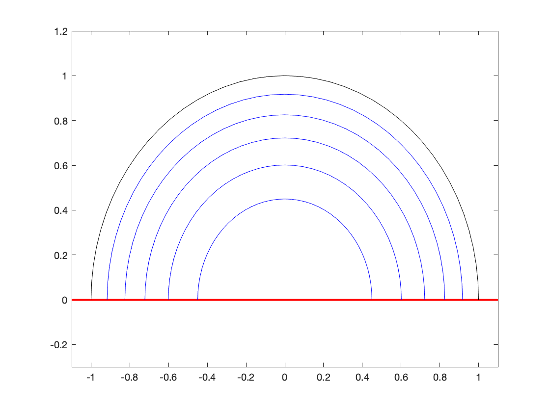
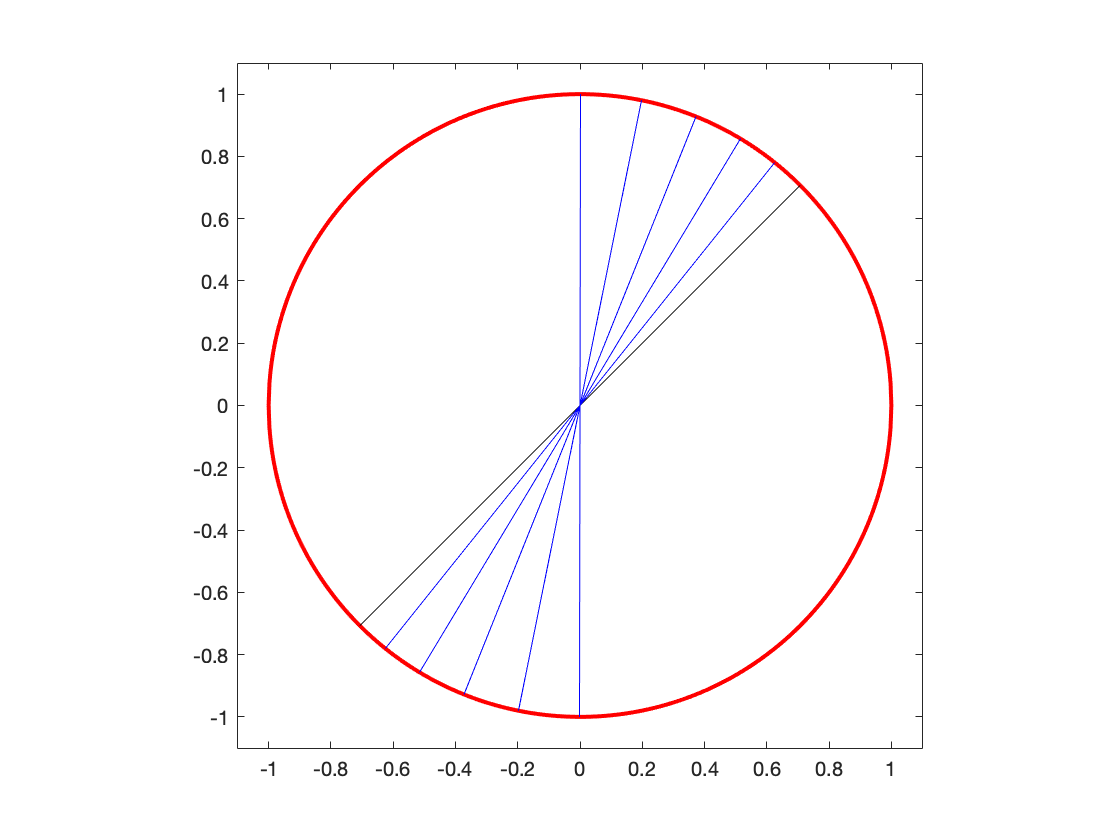
Figure 1: $\vec{X}^{n}$ at $t^{n}=0,0.08,0.16,0.24,0.32,0.4$ for the shrinking semi-circle (left), and $t^{n}=0,0.1,0.2,0.3,0.4,0.5$ for the rotating diameter (right).

Example 2: In the second example we set $T=0.5$ and $\Omega$ to be the unit disc with centre $(0,0)$, such that $\partial\Omega$ is given by $F(x,y)=\frac{1}{2}\left(x^{2}+y^{2}-1\right)$. In contrast to the previous example this example has been constructed so that $|\nabla F(p)|=1$ is only satisfied on $\partial\Omega$. By setting $f(\rho,t)=\frac{4(\rho-\frac{1}{2})}{(1-2t)^{2}+1}$ the explicit solution is given by

$$\vec{x}(\rho,t)=\frac{2(\rho-\frac{1}{2})}{\sqrt{(1-2t)^{2}+1}}\left(1-2t,1\right)^{T},$$

such that $\Gamma(t)$ is a rotating straight line that spans the diameter of $\Omega$. In the right-hand plot of Figure 1 we display: $\vec{X}^{0}$ in black, $\vec{X}^{n}$ at $t^{n}=0.1k$, $k=1,\dots,5$, in blue, and $\partial\Omega$ in red, while Table 3.2 displays the errors $\mathcal{E}_{i}$, $i=1,2$, for $\alpha=1$ (left) and $\alpha=0.5$ (right). As in Example 1, both values of $\alpha$ exhibit eocs close to four, with the errors obtained using $\alpha=0.5$ being smaller than those obtain using $\alpha=1$. However the difference in the errors for the two values of $\alpha$ in this example is much smaller than the difference in the errors for the two values of $\alpha$ in Example 1, we believe that this is due to the fact that in this example $\vec{x}$ is a linear function.

To demonstrate Remark 1 in Section 2, we include Table 3.2 in which we display errors obtained using the scheme in DE98 . In particular we display $\mathcal{E}_{i}$, $i=1,2,3$, with

$$\mathcal{E}_{3}:=\sup_{n=0,\dots,N}\sup_{j=0,\cdots,J}|F(\vec{X}^{n}_{j})|.$$

Comparing the errors in Tables 3.2 and 3.2 we see that the magnitude of the errors for the Newton scheme, (14a)-(14d), are significantly smaller than the errors for the linear scheme in DE98 .

Table 2: Errors and eocs for the rotating diameter with $\alpha=1$ (left) and $\alpha=0.5$ (right).

$J$	$N$	$\mathcal{E}_{1}\times e^{-4}$	$eoc_{1}$	$\mathcal{E}_{2}\times e^{-5}$	$eoc_{2}$
10	50	1.440	-	3.040	-
20	200	0.09198	red3.97	0.1925	red3.98
40	800	0.005780	red3.99	0.01207	red4.00
80	3200	0.0003617	red4.00	0.0007552	red4.00

$J$	$N$	$\mathcal{E}_{1}\times e^{-4}$	$eoc_{1}$	$\mathcal{E}_{2}\times e^{-5}$	$eoc_{2}$
10	50	1.181	-	2.710	-
20	200	0.07459	red3.98	0.1716	red3.98
40	800	0.004674	red4.00	0.01076	red4.00
80	3200	0.0002923	red4.00	0.0006727	red4.00

Table 3: Errors and eocs for the rotating diameter for scheme proposed in DE98 .

$J$	$N$	$\mathcal{E}_{1}\times e^{-4}$	$eoc_{1}$	$\mathcal{E}_{2}\times e^{-5}$	$eoc_{2}$	$\mathcal{E}_{3}\times e^{-3}$	$eoc_{3}$
10	50	43.83		76.20		5.771
20	200	3.175	red3.79	5.442	red3.81	1.563	red0.94
40	800	0.2076	red3.93	0.3542	red3.94	0.3989	red0.99
80	3200	0.01317	red3.98	0.02243	red3.98	0.1003	red1.00

3.3 Experimental order of convergence of the coupled scheme (11)-(13)

We conclude our numerical results by investigating the experimental order of convergence of the coupled scheme (11)-(13). In addition to monitoring the errors $\mathcal{E}_{i}$, $i=1,2$, we also monitor

$$\mathcal{E}_{4}:=\sup_{n=0,\dots,N}\|I^{h}(w^{n})-W^{n}\|_{L^{2}(\mathbb{I})}^{2},\quad\mathcal{E}_{5}:=\sum_{n=1}^{n}\Delta t_{n}\|I^{h}(w^{n}_{\rho})-W^{n}_{\rho}\|_{L^{2}(\mathbb{I})}^{2}.$$

We adopt the same set-up as in Example 2, with $T=0.5$ and $\Omega$ being the unit disc with centre $(0,0)$, such that $\partial\Omega$ is given by $F(x,y)=\frac{1}{2}\left(x^{2}+y^{2}-1\right)$. Setting $f(\rho,t)=\frac{4\left(\rho^{2}-\frac{w(\rho,t)}{1-t}-\frac{1}{2}\right)}{(1-2t)^{2}+1}$ and $g=\frac{t-1}{2}-\frac{w(\rho,t)}{1-t}$, the explicit solution is given by

$$x=\frac{2(\rho-\frac{1}{2})}{\sqrt{(1-2t)^{2}+1}}(1-2t,1)^{T}~{}~{}\text{and}~{}~{}w=(1-t)\rho(\rho-1),$$

such that $w$ describes a shrinking parabola and, as in Example 2, $\Gamma(t)$ is a rotating straight line that spans the diameter of $\Omega$. In the left-hand plot of Figure 2 we display: $\vec{X}^{0}$ in black, $\vec{X}^{n}$, at $t^{n}=0.1k$, $k=1,\dots,5$, in blue, and $\partial\Omega$ in red, while in the right-hand plot we display: $W^{0}$ in black and $W^{n}$, at $t^{n}=0.1k$, $k=1,\dots,5$ in blue. In Table 3.3 we present the experimental order of convergence for the errors obtained using $\alpha=0.5$, we do not present the errors for $\alpha=1$ since they are very similar to those obtained using $\alpha=0.5$. For all the four errors we see eocs close to four.

Remark 2

In the three examples presented above if we take $\Delta t=Ch$ we observe eocs close to two rather than the eocs close to four that we observe above for $\Delta t=Ch^{2}$. Similar convergence behaviour was observed in BDS17 .

Table 4: Errors and eocs for the parabola defined on the rotating diameter with $\alpha=0.5$.

$J$	$N$	$\mathcal{E}_{1}\times e^{-4}$	$eoc_{1}$	$\mathcal{E}_{2}\times e^{-5}$	$eoc_{2}$	$\mathcal{E}_{4}\times e^{-6}$	$eoc_{4}$	$\mathcal{E}_{5}\times e^{-6}$	$eoc_{5}$
10	50	1.205	-	3.756	-	1.207	-	3.073	-
20	200	0.07643	red3.98	0.2453	red3.94	0.07829	red3.95	0.2010	red3.93
40	800	0.004795	red3.99	0.01551	red3.98	0.004937	red3.99	0.01271	red3.98
80	3200	0.0003000	red4.00	0.0009721	red4.00	0.0003093	red4.00	0.0007967	red4.00

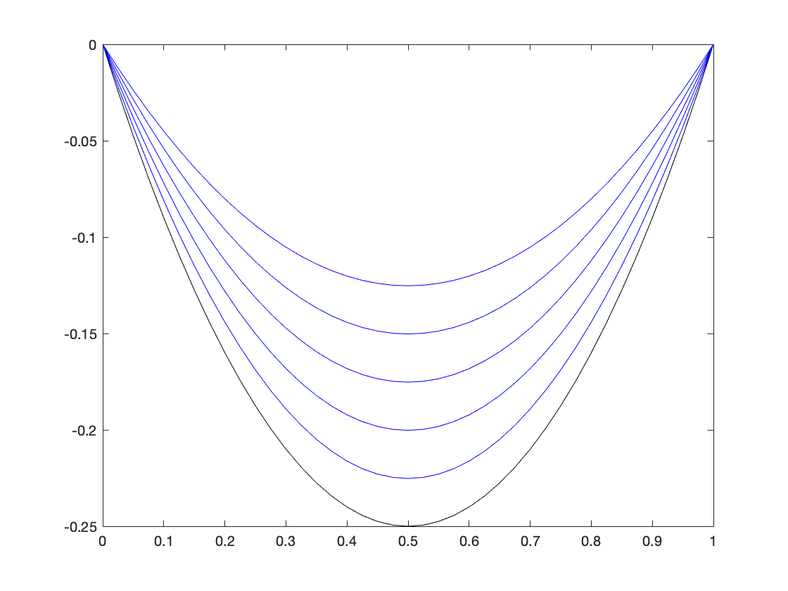
Figure 2: $\vec{X}^{n}$ at $t^{n}=0,0.1,0.2,0.3,0.4,0.5$ for the rotating diameter (left) and $W^{n}$ at $t^{n}=0,0.1,0.2,0.3,0.4,0.5$ for the shrinking parabolic (right).

- (1) J.W. Barrett, K. Deckelnick and V. Styles: Numerical analysis for a system coupling curve evolution to reaction diffusion on the curve. SIAM Journal on Numerical Analysis, vol 55 (2017), p.1080–1100
- (2) J.W. Barrett, H. Garcke and R. Nürnberg: On the variational approximation of combined second and fourth order geometric evolution equations SIAM J. Scientific Comput. 29, (2007), 1006-1041.
- (3) J.W. Barrett, H. Garcke and R. Nürnberg: The approximation of planar curve evolutions by stable fully implicit finite element schemes that equidistribute. Numerical Methods for Partial Differential Equations, 27 (2011), pp. 1–30.
- (4) K. Deckelnick and G. Dziuk: On the approximation of the curve shortening flow. Calculus of Variations, Applications and Computations, (Pitman, 1995), p.100–108
- (5) K. Deckelnick and C.M. Elliott: Finite element error bounds for a curve shrinking with prescribed normal contact to a fixed boundary. IMA Journal of Numerical Analysis, vol 18 (Oxford University Press, 1998), p.635–654
- (6) K. Deckelnick, C.M. Elliott and V. Styles: Numerical diffusion-induced grain boundary motion. Interfaces and Free Boundaries, vol 3 (1998), p.393–414
- (7) G. Dziuk: Convergence of a semi-discrete scheme for the curve shortening flow. Mathematical Models and Methods in Applied Sciences, vol 4 (World Scientific, 1994), p.589–606
- (8) C.M. Elliott and H. Fritz: On approximations of the curve shortening flow and of the mean curvature flow based on the DeTurck trick. IMA Journal of Numerical Analysis, vol 37 (2016), p.543–603
- (9) P. Pozzi and B. Stinner: Curve shortening flow coupled to lateral diffusion. Numerische Mathematik, vol 135 (Springer, 2017), p.1171–1205