Performances of the mixed virtual element method on complex grids for underground flow

Abstract

The numerical simulation of physical processes in the underground frequently entails challenges related to the geometry and/or data. The former are mainly due to the shape of sedimentary layers and the presence of fractures and faults, while the latter are connected to the properties of the rock matrix which might vary abruptly in space. The development of approximation schemes has recently focused on the overcoming of such difficulties with the objective of obtaining numerical schemes with good approximation properties. In this work we carry out a numerical study on the performances of the Mixed Virtual Element Method (MVEM) for the solution of a single-phase flow model in fractured porous media. This method is able to handle grid cells of polytopal type and treat hybrid dimensional problems. It has been proven to be robust with respect to the variation of the permeability field and of the shape of the elements. Our numerical experiments focus on two test cases that cover several of the aforementioned critical aspects.

1 Introduction

The numerical simulation of subsurface flows is of paramount importance in many environmental and energy related applications such as the management of groundwater resources, geothermal energy production, subsurface storage of carbon dioxide. The physical processes are usually modeled, under suitable assumptions, by Darcy’s law and its generalization to multiphase flow.

In spite of the simplicity of the Darcy model the simulation of subsurface flow is often a numerical challenge due to the strong heterogeneity of the coefficients, porosity and permeability of the porous medium, and to the geometrical complexity of the domains of interest. At the spatial scale of reservoirs, or sedimentary basins, the porous medium has a layered structure due to the deposition and erosion of sediments, and tectonic stresses can create, over millions or years, deformations, folds, faults and fractures. In realistic cases the construction of a computational grid that honours the geometry of layers and a large number of fractures is not only a difficult task, but can also give poor results in terms of quality, creating, for instance, very small or badly shaped elements in the vicinity of the interfaces.

In the framework of Finite Volume and Finite Elements methods one possibility is to consider formulations that allow for coarse and regular grids cut by the interfaces in arbitrary ways. The Embedded Discrete Fracture Model, for instance, [45, 51, 41], can represent permeable fracture that cut the background grid by adding additional trasmissibilities in the matrix resulting from the Finite Volumes discretization; on the other hand the eXtended Finite Element Method can be used to generalize a classical FEM discretization allowing for discontinuities inside an element of the grid, see for example [22, 30, 25, 29] for the application of this technique to Darcy’s problem.

A promising alternative consists in the use of numerical methods that are robust in the presence of more general grids, in particular polygonal/polyhedral grids and that impose mild restriction on element shape: this is the case for the Virtual Element Method (VEM), introduced in [7, 18, 8] and successfully applied now to a variety of problems, including elliptic problems in mixed form which is the case of the Darcy model considered in this work. See also [11, 10, 38, 36, 39]. By avoiding the explicit construction of basis function VEM can indeed handle very general grids, which might be useful in the aforementioned cases where the heterogeneity of the medium and the presence of internal interfaces pose constraints to grid generation. In the context of porous media simulations, mixed methods, i.e. methods that consider both velocity and pressure as unknowns of the problem, are of particular interest since they provide a good approximation of pressure as well as an accurate (and conservative) velocity field. For these reasons, we focus our attention on the Mixed Virtual Element Method (MVEM).

The aim of this work is to consider practical grid generation strategies to deal with such complex geometries and to test the performances of the MVEM method on the different types of grid proposed. In particular, we want to investigate the impact of grid type and element shape on properties of the linear system such as sparsity and condition number, and eventually compare the errors. To this aim we will consider two test cases from the literature, in particular two layers from the well-known 10^th SPE Comparative Solution Project (SPE10) dataset, described in [21], characterized by a complex permeability field, and a test case for fractured media taken from [28]. We focus our attention on grid generation strategies that can be applicable in realistic cases: if it is certainly true that MVEM can handle general polytopal grid the construction of such grids is often a difficult task. For this reason, in addition to classical Delaunay triangular grids we consider the case of Voronoi grids, rectangular Cartesian grids cut by fractures, and grids generated by agglomeration. This latter strategy can be applied as a post-processing to all other grid types with the advantage of reducing the number of unknowns. For the numerical implementation of the test cases we have used the publicly available library PorePy [44].

The paper is structured as follows: in Section 2 we present the mathematical model, i.e. the single phase Darcy model in the presence of fractures approximated as codimension 1 interfaces. Section 3 is devoted to the weak formulation of the problem just introduced. Section 4 introduces the numerical discretization by the Virtual Element method, while in Section 5 we describe the grid generation strategies used in the paper. Section 6 presents the numerical tests, and Section 7 is devoted to conclusions.

2 Governing equations

We now introduce the mathematical models considered in this work. The realistic modeling of subsurface flows requires a complex set of non-linear equations and constitutive laws, however one of the key ingredient (upon a suitable linearisation) is the single-phase flow model for a porous media based on Darcy’s law and mass conservation. We are here studying this model, keeping in mind that it might be seen as a part of a more complex model. In addition, it is of our interest to consider also fractures in the porous media, and this calls for a more sophisticated approach.

As already mentioned, we set our study in a saturated porous medium represented by the domain $\Omega\subset\mathbb{R}^{2}$. The boundary of $\Omega$, indicated with $\partial\Omega$, is supposed regular enough (e.g. Lipschitz continuous). The boundary is divided into two disjoint parts $\partial_{u}\Omega$ and $\partial_{p}\Omega$ such that $\accentset{\circ}{\partial_{u}\Omega}\cap\accentset{\circ}{\partial_{p}\Omega}=\emptyset$ and $\overline{\partial_{u}\Omega}\cup\overline{\partial_{p}\Omega}=\overline{\partial\Omega}$. These portions of the boundary will be used to define boundary conditions.

2.1 Single-phase flow in the bulk domain

We briefly recall the mathematical model of single-phase flow in porous media, referring to classical results in literature, see [5], for details. We are interested in the computation of the vector field Darcy velocity $\bm{u}$ and scalar field pressure $p$, which are solutions of the following problem

$$\begin{aligned} &\begin{aligned} &\bm{u}+K\nabla p=\bm{0}\\ &\nabla\cdot\bm{u}=f\end{aligned}&&\text{in }\Omega,\\ &\bm{u}\cdot\bm{n}_{\partial}=\overline{u}&&\text{on }\partial_{u}\Omega,\\ &p=\overline{p}&&\text{on }\partial_{p}\Omega.\end{aligned}$$ (1)

The parameter $K$ is the $2\times 2$ permeability tensor, which is symmetric and positive definite. For simplicity, the dynamic viscosity of the fluid is included into $K$. The source or sink term is named $f$. Finally, $\bm{n}_{\partial}$ is the outward unit normal on $\partial\Omega$, $\overline{u}$ and $\overline{p}$ given boundary data.

We recall that the permeability tensor, for real applications, may vary several order of magnitude from region to region (i.e., grid cells) and can be discontinuous.

2.2 Fracture flow

We are interested in the simulation of single-phase flow in porous media in the presence of fractures. For simplicity we start with one single fracture. The model we are considering is the result of a model reduction procedure that approximates the fracture as a lower dimensional object and derives new equations and coupling conditions for the Darcy velocity and pressure both in the fracture and surrounding porous medium. More details on this subject can be found in the following, not exhaustive, list of works [3, 46, 22, 30, 56, 17, 39, 4, 31, 15, 19, 58, 49, 13].

In the following the fracture is indicated with $\gamma$, and quantities related to the porous media and the fracture are indicated with the subscript $\Omega$ and $\gamma$, respectively. The fracture is described by a planar surface with normal vector denoted by $\bm{n}$, which also defines a positive and negative side of $\gamma$, indicated as $\gamma^{+}$ and $\gamma^{-}$, see Figure 1 as an example. Given a field $u$ in $\Omega\setminus\gamma$ we indicate its trace on $\gamma^{+}$ and $\gamma^{-}$ as ${\operatorname{tr}}u_{+}$ and ${\operatorname{tr}}u_{-}$, respectively.

Figure 1: Hybrid-dimensional representation of a fracture immersed in a porous media.

The fracture is characterized by an aperture $\epsilon_{\gamma}$ which, in the reduced model where the fracture has co-dimension one, is only a model parameter. Finally, if the fracture touches the boundary we can apply natural or essential given boundary conditions; we denote as $\partial_{p}\gamma$ and $\partial_{u}\gamma$ the portions of $\partial\gamma$ where pressure and velocity are imposed. We assume that $\accentset{\circ}{\partial_{p}\gamma}\cap\accentset{\circ}{\partial_{u}\gamma}=\emptyset$ as well as ${\partial_{p}\gamma}\cup{\partial_{u}\gamma}={\partial\gamma}$. If a fracture tip does not touch the physical boundary a no-flow condition is imposed, so in this case we assume that the immersed tip belongs to $\partial_{u}\gamma$ with an homogeneous condition.

We recall the system of equations that will be used in the sequel. In the bulk porous medium $\Omega\setminus\gamma$ the problem is governed by the classic Darcy’s equations already presented in (1), which we rewrite using the subscript $\Omega$ to identify quantities in $\Omega\setminus\gamma$

$$\begin{aligned} &\begin{aligned} &\bm{u}_{\Omega}+K_{\Omega}\nabla p_{\Omega}=\bm{0}\\ &\nabla\cdot\bm{u}_{\Omega}=f_{\Omega}\end{aligned}&&\text{in }\Omega\setminus\gamma,\\ &\bm{u}_{\Omega}\cdot\bm{n}_{\partial}=\overline{u}_{\Omega}&&\text{on }\partial_{u}\Omega\setminus\partial\gamma,\\ &p_{\Omega}=\overline{p}_{\Omega}&&\text{on }\partial_{p}{\Omega}\setminus\partial\gamma.\end{aligned}$$ (2a)

We assume that also the flow in the fracture is governed by Darcy’s law, however the differential operators operate now on the tangent space. Yet, for the sake of simplicity, with an abuse of notation we use the same symbols to denote them. The system of equations in the fracture is then given by

$$\begin{aligned} &\begin{aligned} &\epsilon_{\gamma}^{-1}\bm{u}_{\gamma}+K_{\gamma}\nabla p_{\gamma}=\bm{0}\\ &\nabla\cdot\bm{u}_{\gamma}-{\operatorname{tr}}\bm{u}_{+}\cdot\bm{n}+{\operatorname{tr}}\bm{u}_{-}\cdot\bm{n}=f_{\gamma}\end{aligned}&&\text{in }\gamma,\\ &\bm{u}_{\gamma}\cdot\bm{n}_{\partial}=\overline{u}_{\gamma}&&\text{on }\partial_{u}\gamma,\\ &p_{\gamma}=\overline{p}_{\gamma}&&\text{on }\partial_{p}\gamma.\end{aligned}$$ (2b)

Here, $$\overline{u}_{\gamma} \overline{p}_{\gamma} \partial_{u}\gamma \overline{u}_{\gamma}=0 K_{\gamma} \gamma K_{\gamma} \gamma$$ and are given boundary data, and we recall that possible fracture tips are in with . The parameter is the tangential effective permeability in . In the 2D setting, where the reduced fracture model is one-dimensional, is a positive quantity. In the 3D setting, it may be in general a rank-2 symmetric and positive tensor. We may note in the equation representing the conservation of mass the presence of an additional term that describes the flux exchange with the surrounding porous media. To close the problem we need to complete the coupling between fracture and bulk, and we consider the following Robin-type condition on both sides of

$$\epsilon_{\gamma}{\operatorname{tr}}\bm{u}_{\pm}\cdot\bm{n}\pm\kappa_{\gamma}(p_{\gamma}-{\operatorname{tr}}p_{\pm})=0\quad\text{on }\gamma^{\pm},$$ (2c)

with $$\kappa_{\gamma}>0$$ being the normal effective permeability. Problem (2) consists of the system of equations that describe the Darcy velocity and pressure in both the fracture and surrounding porous medium. An analysis may be found, for instance, in [31] or [38].

The case of $N>1$ non-intersecting fractures the problem is analogous to the one just described where $\gamma=\cup_{i=1}^{N}\gamma_{i}$. However, if two or more fractures intersect we need to introduce new conditions to describe the flux interchange between connected fractures. At each intersection $\iota$ we denote with $I_{\iota}$ the set of intersecting fractures and we consider the following conditions on $\iota$,

$$\begin{cases}\epsilon_{\iota}\alpha_{j}{\operatorname{tr}}\bm{u}_{j}\cdot\bm{t}_{j}+\kappa_{\iota}(p_{\iota}-{\operatorname{tr}}p_{j})=0\quad\forall\gamma_{j}\in I_{\iota}\\ \displaystyle\sum_{\gamma_{j}\in I_{\iota}}\alpha_{j}{\operatorname{tr}}\bm{u}_{j}\cdot\bm{t}_{j}=0\end{cases}\quad\text{on }\iota,$$ (3)

where $\epsilon_{\iota}$ is the measure of the intersection, $p_{\iota}$ is the pressure at the intersection, $\kappa_{\iota}$ is the permeability at the intersection and $\alpha\in\{-1,1\}$ depends on the orientation chosen for the normal $\bm{t}_{j}$ to $\partial\gamma_{j}$ at the intersection. Note that $\bm{t}_{j}$ is indeed on the tangent plane of $\gamma_{j}$. System (3) can be simplified by noting that it implies that $p_{\iota}$ is equal to the average of the $p_{j}$.

3 Weak formulation

The numerical scheme that we will present in Section 4 is based on the weak formulation of problem (1) and (2). Therefore, we will present in the following the functional setting and the weak form we have used as basis for the numerical discretization. We indicate with $L^{2}(A)$ the Lebesgue space of square integrable functions on $A$, while $H_{\operatorname{div}}(A)$ is the space of square integrable vector functions whose distributional divergence is in $L^{2}(A)$. They are Hilbert spaces with standard norms and inner products. In particular, we denote with $(\cdot,\cdot)_{A}$ the $L^{2}(A)$-scalar product. Moreover, given a functional space $V$ and its dual $V^{\prime}$ we use $\langle a,b\rangle$, with $a\in V$ and $b\in V^{\prime}$ to denote the duality pairing between the given functional spaces.

3.1 Single-phase bulk flow without fractures

If fractures are not present, the setting is rather standard. For simplicity, we assume homogeneous essential boundary conditions $\overline{u}_{\Omega}=0$, otherwise a lifting technique can be used to recover the original problem. We introduce the following functional spaces for vector and scalar field, respectively,

$$V(\Omega)=\left\{\bm{v}\in H_{\operatorname{div}}(\Omega):\,{\operatorname{tr}}\bm{v}\cdot\bm{n}_{\partial}=0\text{ on }\partial_{u}\Omega\right\}\quad\text{and}\quad Q(\Omega)=L^{2}(\Omega).$$ (4)

Here ${\operatorname{tr}}$ is the normal trace operator ${\operatorname{tr}}:H_{\operatorname{div}}(\Omega)\to H^{-\frac{1}{2}}(\partial_{u}\Omega)$, which is linear and bounded, see [14].

We can now introduce the following bilinear forms and functionals

$$a_{\Omega}:V(\Omega)\times V(\Omega)\rightarrow\mathbb{R}:\quad a_{\Omega}(\bm{u}_{\Omega},\bm{v}_{\Omega})=(H_{\Omega}\bm{u}_{\Omega},\bm{v}_{\Omega})_{\Omega}$$

$$b_{\Omega}:V(\Omega)\times Q(\Omega)\rightarrow\mathbb{R}:\quad b_{\Omega}(\bm{v}_{\Omega},p_{\Omega})=-(\nabla\cdot\bm{v}_{\Omega},q_{\Omega})_{\Omega}$$

$$G_{\Omega}:V(\Omega)\rightarrow\mathbb{R}:\quad G_{\Omega}(\bm{v}_{\Omega})=-\langle{\operatorname{tr}}\bm{v}_{\Omega}\cdot\bm{n}_{\partial},\overline{p}_{\Omega}\rangle$$

$$F_{\Omega}:Q(\Omega)\rightarrow\mathbb{R}:\quad F_{\Omega}(q_{\Omega})=-(f_{\Omega},q_{\Omega})_{\Omega}$$

where $H_{\Omega}=K_{\Omega}^{-1}$. We assume that $K_{\Omega}\in[L^{\infty}(\Omega)]^{2\times 2}$, with $\underline{\alpha}||\bm{y}||^{2}\leq\bm{y}^{T}K\bm{y}\leq\overline{\alpha}||\bm{y}||^{2}$, a.e. in $\Omega$, where $\bm{y}\in\mathbb{R}^{n}$ and $0<\underline{\alpha}\leq\overline{\alpha}$.

Furthermore, we take $\overline{p}_{\Omega}\in H^{\frac{1}{2}}_{00}(\partial_{p}\Omega)$, and $f_{\Omega}\in L^{2}(\Omega)$. Let us note that $a_{\Omega}:\ V(\Omega)\times V(\Omega)\to\mathbb{R}$ is continuous, coercive and symmetric, being $K_{\Omega}$ symmetric.

We can now state the weak formulation of our problem: find $(\bm{u}_{\Omega},p_{\Omega})\in V(\Omega)\times Q(\Omega)$ such that

$$\begin{aligned} &a_{\Omega}(\bm{u}_{\Omega},\bm{v}_{\Omega})+b_{\Omega}(\bm{v}_{\Omega},p_{\Omega})=G(\bm{v}_{\Omega})&&\forall\bm{v}_{\Omega}\in V(\Omega)\\ &b_{\Omega}(\bm{u}_{\Omega},q_{\Omega})=F_{\Omega}(q_{\Omega})&&\forall q_{\Omega}\in Q(\Omega)\end{aligned}.$$ (5)

The previous problem is well posed, provided $|\partial_{p}\Omega|>0$. See, for example, [14] for a proof.

3.2 Fracture flow

We extend now the weak formulation for problem (2), with the simplifying assumption that only one fracture is considered. Its extension to multiple fractures is straightforward, see for example [31, 15]. Also in this case we assume homogeneous essential boundary conditions, otherwise a lifting technique can be used.

We need to introduce the space $H_{\operatorname{div}}(\Omega\setminus\gamma)$ as the space of vector function in $L^{2}(\Omega\setminus\gamma)$ (which may be identified by $L^{2}(\Omega)$ since $\gamma$ has zero measure) whose distributional divergence is in $L^{2}(\Sigma)$ for all measurable $\Sigma\subset(\Omega\setminus\gamma)$. We need also to impose some extra regularity on the trace on $\gamma^{\pm}$, due to the Robin-type condition (2c). The reader may refer to [46, 34, 14] for a more detailed discussion on this matter. In particular, we require that, for a $\bm{v}_{\Omega}\in H_{\operatorname{div}}(\Omega\setminus\gamma)$ , ${\operatorname{tr}}\bm{v}_{+}\cdot\bm{n}\in L^{2}(\gamma)$ and ${\operatorname{tr}}\bm{v}_{-}\cdot\bm{n}\in L^{2}(\gamma)$, where ${\operatorname{tr}}$ here indicates the trace of $\bm{v}$ on the two sides of the fracture. This space is equipped with the inner product

$$(\bm{u},\bm{v})_{H_{\operatorname{div}}(\Omega\setminus\gamma)}=(\bm{u},\bm{v})_{\Omega}+(\nabla\cdot\bm{u},\nabla\cdot\bm{v})_{\Omega}+({\operatorname{tr}}\bm{u}_{+}\cdot\bm{n},{\operatorname{tr}}\bm{v}_{+}\cdot\bm{n})_{\gamma}+({\operatorname{tr}}\bm{u}_{-}\cdot\bm{n},{\operatorname{tr}}\bm{v}_{-}\cdot\bm{n})_{\gamma},$$

and induced norm. The new space for vector fields in the bulk is given by

$$\hat{V}(\Omega)=\left\{\bm{v}_{\Omega}\in H_{\operatorname{div}}(\Omega\setminus\gamma):\,{\operatorname{tr}}\bm{v}_{\Omega}\cdot\bm{n}_{\partial}=0\text{ on }\partial_{u}\Omega\right\}.$$

The functional spaces for vector and scalar fields defined on the fracture are

$$V(\gamma)=\left\{\bm{v}_{\gamma}\in H_{\operatorname{div}}(\gamma):\,{\operatorname{tr}}\bm{v}_{\gamma}\cdot\bm{n}_{\partial}=0\right\}\quad\text{and}\quad Q(\gamma)=L^{2}(\gamma),$$

where in this case the trace operator in $V(\gamma)$ is given by ${\operatorname{tr}}:H_{\operatorname{div{}}}(\gamma)\rightarrow H^{-\frac{1}{2}}(\partial_{u}\gamma)$. Note that in the case of 2D problems like the ones treated in this work, $V(\gamma)$ is in fact a subspace of $H^{1}(\gamma)$ and the trace reduces to the value at the boundary point.

We introduce now the bilinear forms and functional for the weak formulation of problem (2). First, we modify the bilinear form $a_{\Omega}$ by taking into account the coupling terms from (2c) as

$$\hat{a}_{\Omega}:\hat{V}(\Omega)\times\hat{V}(\Omega)\rightarrow\mathbb{R}:\quad\hat{a}_{\Omega}(\bm{u}_{\Omega},\bm{v}_{\Omega})=a_{\Omega}(\bm{u}_{\Omega},\bm{v}_{\Omega})_{\Omega}+\sum_{*\in\{+,-\}}(\eta_{\gamma}{\operatorname{tr}}\bm{u}_{*}\cdot\bm{n},{\operatorname{tr}}\bm{u}_{*}\cdot\bm{n})_{\gamma}$$

where $\eta_{\gamma}=\epsilon_{\gamma}\kappa_{\gamma}^{-1}$ and we have assumed that $\eta_{\gamma}\in L^{\infty}(\gamma)$. Second, the bilinear forms associated with the fracture are given by

$$a_{\gamma}:V(\gamma)\times V(\gamma)\rightarrow\mathbb{R}:\quad a_{\gamma}(\bm{u}_{\gamma},\bm{v}_{\gamma})=(H_{\gamma}\bm{u}_{\gamma},\bm{v}_{\gamma})_{\gamma}$$

$$b_{\gamma}:V(\gamma)\times Q(\gamma)\rightarrow\mathbb{R}:\quad b_{\gamma}(\bm{v}_{\gamma},p_{\gamma})=-(\nabla\cdot\bm{v}_{\gamma},p_{\gamma})_{\gamma}$$

$$G_{\gamma}:V(\gamma)\rightarrow\mathbb{R}:\quad G_{\gamma}(\bm{v}_{\gamma})=-\langle{\operatorname{tr}}\bm{v}_{\gamma}\cdot\bm{n}_{\partial},\overline{p}_{\gamma}\rangle$$

$$F_{\gamma}:V(\gamma)\times\mathbb{R}:\quad F_{\gamma}(q_{\gamma})=-(f_{\gamma},q_{\gamma})_{\gamma}$$

where we have $H_{\gamma}^{-1}=\epsilon_{\gamma}K_{\gamma}$ and we have assumed that $H_{\gamma}\in L^{\infty}(\gamma)$, $\overline{p}_{\gamma}\in H^{\frac{1}{2}}(\partial_{p}\gamma)$, and $f_{\gamma}\in L^{2}(\gamma)$. Third, we introduce the bilinear forms responsible for the flux exchange between the fracture and the bulk medium

$$c^{\pm}:\hat{V}(\Omega)\times Q(\gamma)\rightarrow\mathbb{R}:\quad c^{\pm}(\bm{u}_{\Omega},q_{\gamma})=\pm({\operatorname{tr}}\bm{u}_{\pm}\cdot\bm{n},q_{\gamma})_{\gamma}$$

$$c:\hat{V}(\Omega)\times Q(\gamma)\rightarrow\mathbb{R}:\quad c(\bm{u}_{\Omega},q_{\gamma})=\sum_{*\in\{+,-\}}c^{*}(\bm{u}_{\Omega},q_{\gamma}).$$

We finally can write the weak formulation for problem (2): find $(\bm{u}_{\Omega},p_{\Omega},\bm{u}_{\gamma},p_{\gamma})\in\hat{V}(\Omega)\times Q(\Omega)\times V(\gamma)\times Q(\gamma)$ such that

$$\begin{aligned} &\hat{a}_{\Omega}(\bm{u}_{\Omega},\bm{v}_{\Omega})+b_{\Omega}(\bm{v}_{\Omega},p_{\Omega})+c(\bm{v}_{\Omega},p_{\gamma})=G_{\Omega}(\bm{v}_{\Omega})&&\forall\bm{v}_{\Omega}\in\hat{V}(\Omega)\\ &b_{\Omega}(\bm{u}_{\Omega},q_{\Omega})=F_{\Omega}(q_{\Omega})&&\forall q_{\Omega}\in Q(\Omega)\\ &a_{\gamma}(\bm{u}_{\gamma},\bm{v}_{\gamma})+b_{\gamma}(\bm{v}_{\gamma},p_{\gamma})=G_{\gamma}(\bm{v}_{\gamma})&&\forall\bm{v}_{\gamma}\in V(\gamma)\\ &b_{\gamma}(\bm{u}_{\gamma},q_{\gamma})+c(\bm{u}_{\Omega},q_{\gamma})=F_{\gamma}(q_{\gamma})&&\forall q_{\gamma}\in Q(\gamma)\end{aligned}$$ (6)

The reader can refer to [22, 30, 25] for proofs of the well posedness of the problem, provided suitable boundary conditions.

4 Numerical approximation by MVEM

The challenges in terms of heterogeneity of physical data and complexity of the geometry due to the presence of fractures influence the choice of the numerical scheme. A possible choice is the mixed finite element method, see [54, 55, 14]. However, this class of methods, capable of providing accurate results for pressure and velocity fields, even in the presence of high heterogeneities, requires grids made either of simplexes (triangles of tetrahedra) or quad/hexahedra. This can be inefficient for the problem at hand, where instead methods able to operate on grids formed by arbitrary polytopes are rather appealing. For this reason finite volume schemes, see [26] for a review, are very much used in practice. However, they normally treat the primal formulation and require good quality grids to obtain an accurate solution and a good reconstruction of the velocity field. Indeed, it is known that convergence of the method is guaranteed only if the grid has special properties.

Therefore, we focus here our attention on the low-order Mixed Virtual Element Method, a numerical schemes that operates on polytopal grids and that has shown to be rather robust with respect to irregularities in the data and in the computational grid. We consider first the case of porous medium without fractures, focusing on problems with highly heterogeneous permeability, and then the case of a fractured porous medium, using the model described in Subsection 4.2.

The actual implementation in PorePy adopts a flux mortar technique that allows non-conforming coupling between inter-dimensional grids. We do not exploit the possibility of having grids non-conforming to the fractures in this work, nevertheless in Subsection 4.2 we will describe the mortar approach more in detail.

4.1 Bulk flow without fractures

In this part we present the MVEM discretization of problem (5). A key point of the virtual method is to use an implicit definition of suitable basis functions, and obtain computable discrete local matrices by manipulating the different terms in the weak formulation appropriately. In this work we consider only the low order case, yet the method can be extended to higher order formulations.

We indicate the computational grid, approximation of $\Omega$, as $\mathcal{T}(\Omega)$. We assume that $\Omega$ has polygonal boundary, so that $\mathcal{T}(\Omega)$ covers $\Omega$ exactly. The set of faces of $\mathcal{T}(\Omega)$ is denoted as $\mathcal{E}(\Omega)$, with the distinction between the internal and boundary faces indicated by $\mathcal{E}({\accentset{\circ}{\Omega}})$ and $\mathcal{E}({\partial\Omega}$), respectively. We also specify the edges on a specific portion of the boundary of $\Omega$ as $\mathcal{E}(\partial_{u}\Omega)$ and $\mathcal{E}(\partial_{p}\Omega)$. We clearly have $\mathcal{E}(\accentset{\circ}{\Omega})\cup\mathcal{E}(\partial\Omega)=\mathcal{E}(\Omega)$ as well as $\mathcal{E}(\accentset{\circ}{\Omega})\cap\mathcal{E}(\partial\Omega)=\emptyset$. In the sequel, we generally indicate as $C\in\mathcal{T}(\Omega)$ a grid cell and $e\in\mathcal{E}(\Omega)$ a face between two cells. Element $C$ can be a generic polygon (polyhedra in the 3D case).

We introduce the finite dimensional subspaces, approximation of the continuous spaces given in (4), as

$$V_{h}(\Omega)=\left\{\bm{v}_{\Omega}\in V(\Omega):\,\nabla\cdot\bm{v}_{\Omega}|_{C}\in\mathbb{P}_{0}(C)\text{ and }\nabla\times\bm{v}_{\Omega}|_{C}=\bm{0},\,\forall C\in\mathcal{T}(\Omega),\right.$$

$$\left.\,{\operatorname{tr}}\bm{v}_{\Omega}\cdot\bm{n}_{e}\in\mathbb{P}_{0}(e),\,\forall e\in\mathcal{E}(\Omega)\right\},$$

with $\mathbb{P}_{0}(X)$ being the space of constant polynomials on $X$, while ${\operatorname{tr}}$ and $\bm{n}_{e}$ the trace and the normal associated to edge $e$. For the scalar field we set

$$Q_{h}({\Omega})=\left\{q_{\Omega}\in Q(\Omega):\,q_{\Omega}|_{C}\in\mathbb{P}_{0}(C)\,\forall C\in\mathcal{T}(\Omega)\right\}.$$

Clearly $V_{h}({\Omega})\subset V(\Omega)$ and $Q_{h}({\Omega})\subset Q(\Omega)$. The degrees of freedom associated with $V_{h}({\Omega})$ and $Q_{h}({\Omega})$ are one scalar value for each face and one scalar value for each cell, respectively. More precisely, if we generically indicate with $\operatorname*{\operatorname{dof}}_{i}$ the functional associated with the $i$-th degree of freedom, we have, for a $\bm{v}_{\Omega}\in V_{h}(\Omega)$ and a $q_{\Omega}\in Q_{h}({\Omega})$

$$\operatorname*{\operatorname{dof}}_{i}\bm{v}_{\Omega}={\operatorname{tr}}\bm{v}_{\Omega}\cdot\bm{n}_{e_{i}}\quad\text{and}\quad\operatorname*{\operatorname{dof}}_{i}q_{\Omega}=q_{\Omega}|_{C_{i}},$$

where $e_{i}$ and $C_{i}$ are the $i$-th edge and cell, respectively, and ${\operatorname{tr}}$ now indicates the trace associated to the edge $e_{i}$.

Moreover, we can observe that in case of triangular grids $V_{h}({\Omega})$ coincides with $\mathbb{RT}_{0}(\Omega)$, so the former can be viewed as a generalization of the well known Raviart-Thomas finite elements.

By performing exact integration, the numerical approximation of the bilinear form $b_{\Omega}$ and of the functionals $G_{\Omega}$, $F_{\Omega}$ are computable with the given definition of the discrete spaces. However, for the term ${a}_{\Omega}$ we need further manipulations to obtain a computable expression. To this purpose, we define a suitable subspace of $V_{h}(\Omega)$, defined as

$$\mathcal{V}_{h}(\Omega)=\left\{\bm{v}_{\Omega}\in V_{h}(\Omega):\,\bm{v}_{\Omega}|_{C}=K_{C}\nabla v_{C}\text{ for a }v_{C}\in\mathbb{P}_{1}(C)\forall C\in\mathcal{T}(\Omega)\right\},$$

where $K_{C}$ is a suitable constant approximation of $K_{\Omega}|_{C}$, and we define a projection operator $\Pi_{\Omega}:V_{h}(\Omega)\rightarrow\mathcal{V}_{h}(\Omega)$ so that for a $\bm{v}\in V_{h}(\Omega)$ we have

$$a_{\Omega}(\bm{v}-\Pi_{\Omega}\bm{v},\bm{w})=0,\quad\forall\bm{w}\in\mathcal{V}_{h}(\Omega).$$

We now set $T_{\Omega}=I-\Pi_{\Omega}$, where $T_{\Omega}:V_{h}(\Omega)\rightarrow\mathcal{V}_{h}^{\perp}(\Omega)$ and the orthogonality condition is governed by the bilinear form $a_{\Omega}$, which, being symmetric, continuous and coercive, defines an inner product. Indeed, from the definition of $\Pi_{\Omega}$ we have $a_{\Omega}(T_{\Omega}\bm{v}_{\Omega},\Pi_{\Omega}\bm{w}_{\Omega})=0$ for all $\bm{v}_{\Omega},\bm{w}_{\Omega}\in V_{h}(\Omega)$. Considering this fact, we have the following decomposition

$$a_{\Omega}(\bm{u}_{\Omega},\bm{v}_{\Omega})=a_{\Omega}((\Pi_{\Omega}+T_{\Omega})\bm{u}_{\Omega},(\Pi_{\Omega}+T_{\Omega})\bm{v}_{\Omega})=a_{\Omega}(\Pi_{\Omega}\bm{u}_{\Omega},\Pi_{\Omega}\bm{v}_{\Omega})+a_{\Omega}(T_{\Omega}\bm{u}_{\Omega},T_{\Omega}\bm{v}_{\Omega}).$$

Now, thanks to the definition of $\mathcal{V}_{h}(\Omega)$ the first term is computable in terms of the degrees of freedom, see for instance [37], but not the second one. However, since it gives the contribution of $a_{\Omega}$ only on $\mathcal{V}_{h}^{\perp}(\Omega)$, it can be approximated with a suitable stabilizing bilinear form $s:V_{h}(\Omega)\times V_{h}(\Omega)\rightarrow\mathbb{R}$, i.e.

$$a_{\Omega}(T_{\Omega}\bm{u}_{\Omega},T_{\Omega}\bm{v}_{\Omega})\approx s_{\Omega}(\bm{u}_{\Omega},\bm{v}_{\Omega}).$$

For more details about $s_{\Omega}$ refer to the works [18, 6, 8, 38, 39, 23]. The form $s_{\Omega}$ must satisfy the following equivalence condition:

$$\exists\upsilon_{*},\upsilon^{*}\in\mathbb{R}^{+}:\quad\upsilon_{*}a_{\Omega}(\bm{u}_{\Omega},\bm{v}_{\Omega})\leq s_{\Omega}(\bm{u}_{\Omega},\bm{v}_{\Omega})\leq\upsilon^{*}a_{\Omega}(\bm{u}_{\Omega},\bm{v}_{\Omega})\quad\forall\bm{u}_{\Omega},\bm{v}_{\Omega}\in V_{h}(\Omega).$$

The illustrate our choice of $s_{\Omega}$, let us denote with $\bm{\varphi}$ a generic element of the basis of $V_{h}(\Omega)$. The stabilization term, in our case, can be computed as

$$s_{\Omega}(\bm{\varphi}_{\theta},\bm{\varphi}_{\chi})=\sum_{C\in\mathcal{T}(\Omega)}{\left\|{H_{\Omega}}\right\|}_{L^{\infty}(C)}\sum_{i=1}^{N_{dof}(C)}\operatorname*{\operatorname{dof}}_{i}(T_{\Omega}\bm{\varphi}_{\theta})\operatorname*{\operatorname{dof}}_{i}(T_{\Omega}\bm{\varphi}_{\chi}),$$ (7)

where $N_{dof}(C)$ is the total number of degrees of freedom for the vector field for the cell $C$ and $\operatorname*{\operatorname{dof}}_{i}$ gives the value of the argument at the $i^{th}$-dof. The $K_{\Omega}$ norm is a scaling factor in order to consider also strong oscillations of physical parameters. With the definition of the stabilization term now all the terms are computable and the global system can be assembled. For more details on the actual computation of the local matrices refer to [38, 7].

4.2 Fracture flow

We introduce now the numerical scheme used for the approximation of problem (6). We consider the notations and terms for the porous media from the previous section. In fact the derivation of the discrete setting for the porous media is similar to what already presented. We focus now on the fracture discretization as well as on the coupling term with the surrounding porous media.

In particular, for the implementation we have chosen PorePy [44], that considers an additional interface $\gamma^{\pm}$ between the fracture and the porous media along with a flux mortar technique to couple domains of different dimensions, allowing also non-conforming grids between the domains. However, to avoid additional complexity we consider only conforming grids so that the mortar variable behaves as a Lagrange multiplier $\lambda_{h}$. The latter is the normal flux exchange from the higher to lower dimensional domain. See Figure 2a as an example. Geometrically i) the interface between the porous media and the fracture, ii) the fracture, and iii) the two interfaces coincide but they are represented by different objects with suitable operators for their coupling. In the case of conforming discretizations these operators simply map the corresponding degrees of freedom, however in the case of non-conforming discretizations projection operators should be considered.

(a) Interfaces

(b) Degrees of freedom

Figure 2: On the left, the hybrid-dimensional representation of a fracture immersed in a porous media with the two interfaces $\gamma^{+}$ and $\gamma^{-}$, in red. On the right, the representation of the degrees of freedom for vector fields.

As done before, we consider the special case of a single fracture, being its generalization straightforward. First of all, the velocity degrees of freedom for the rock matrix in the proximity of the fracture are doubled as Figure 2b shows. We can thus represent ${\operatorname{tr}}\bm{u}_{\pm}\cdot\bm{n}=\lambda^{\pm}_{h}$ for both sides $\pm$ of the fracture itself. The term $\hat{a}_{\Omega}$ involves the actual integration of the basis functions for each grid cells, which is not possible since they are not, in general, analytically known.

Many of the following steps are similar to what already done for the bulk porous media. We introduce a tessellation of $\gamma$ into non-overlapping cells (segments in this case), the grid is indicated with $\mathcal{T}(\gamma)$ and the set of faces (edges) as $\mathcal{E}(\gamma)$. Also in this case, we divide the internal faces and the external faces $\mathcal{E}(\accentset{\circ}{\gamma})$ and $\mathcal{E}(\partial\gamma)$. Moreover, the latter can also be divided into subset depending on the boundary conditions $\mathcal{E}(\partial_{u}\gamma)$ and $\mathcal{E}(\partial_{p}\gamma)$. Clearly, we have $\mathcal{E}(\gamma)=\mathcal{E}(\accentset{\circ}{\gamma})\cup\mathcal{E}(\partial\gamma)$ as well as $\mathcal{E}(\partial_{u}\gamma)\cup\mathcal{E}(\partial_{p}\gamma)=\mathcal{E}(\partial\gamma)$. We introduce the functional spaces for the variables defined on the fracture, for the vector fields we have

$$V_{h}(\gamma)=\left\{\bm{v}_{\gamma}\in V(\gamma):\,\nabla\cdot\bm{v}_{\gamma}|_{C}\in\mathbb{R}\text{ and }\nabla\times\bm{v}_{\gamma}|_{C}=\bm{0}\,\forall C\in\mathcal{T}(\gamma),\,{\operatorname{tr}}\bm{v}_{\gamma}\cdot\bm{n}_{e}\in\mathbb{R}\,\forall e\in\mathcal{E}(\gamma)\right\},$$

while for the scalar fields we consider the discrete space

$$Q_{h}(\gamma)=\left\{q_{\gamma}\in Q(\gamma):\,q_{\gamma}|_{C}\in\mathbb{R}\,\forall C\in\mathcal{T}(\gamma)\right\}.$$

By keeping the same approach as before, we assume exact integration so that the numerical approximation of the bilinear form $b_{\gamma}$ as well as functionals $G_{\gamma}$ and $F_{\gamma}$ are computable with the given definition of the discrete spaces. The term $a_{\gamma}$ is not directly computable, we thus introduce the subspace of $V_{h}(\gamma)$ as

$$\mathcal{V}_{h}(\gamma)=\left\{\bm{v}_{\gamma}\in V_{h}(\gamma):\,\bm{v}_{\gamma}|_{C}=K_{\gamma}|_{C}\nabla v_{C}\text{ for a }v_{C}\in\mathbb{P}_{1}(C)\forall C\in\mathcal{T}(\gamma)\right\}.$$

We introduce the projection operator $\Pi_{\gamma}$ from $V_{h}(\gamma)\rightarrow\mathcal{V}_{h}(\gamma)$ such that for a $\bm{v}\in V_{h}(\gamma)$ we have $a_{\gamma}(\bm{v}-\Pi_{\gamma}\bm{v},\bm{w})=0$ for all $\bm{w}\in\mathcal{V}_{h}$. By introducing the operator $T_{\gamma}=I-\Pi_{\gamma}$, we have the decomposition

$$a_{\gamma}(\bm{u}_{\gamma},\bm{v}_{\gamma})=a_{\gamma}((\Pi_{\gamma}+T_{\gamma})\bm{u}_{\gamma},(\Pi_{\gamma}+T_{\gamma})\bm{v}_{\gamma})=a_{\gamma}(\Pi_{\gamma}\bm{u}_{\gamma},\Pi_{\gamma}\bm{v}_{\gamma})+a_{\gamma}(T_{\gamma}\bm{u}_{\gamma},T_{\gamma}\bm{v}_{\gamma})$$

By the definition of $\mathcal{V}_{h}(\gamma)$ the first term is now computable, while the second term, which is not computable, is replaced by the stabilization term

$$a_{\gamma}(T_{\gamma}\bm{u}_{\gamma},T_{\gamma}\bm{v}_{\gamma})\approx s_{\gamma}(\bm{u}_{\gamma},\bm{v}_{\gamma})$$

with the request that $s_{\gamma}$ scales as $a_{\gamma}$, meaning that

$$\exists\upsilon_{*},\upsilon^{*}\in\mathbb{R}:\quad\upsilon_{*}s_{\gamma}(\bm{u}_{\gamma},\bm{v}_{\gamma})\leq a_{\gamma}(\bm{u}_{\gamma},\bm{v}_{\gamma})\leq\upsilon^{*}s_{\gamma}(\bm{u}_{\gamma},\bm{v}_{\gamma})\quad\forall\bm{u}_{\gamma},\bm{v}_{\gamma}\in V_{h}(\gamma).$$

Denoting an element of the basis of $V_{h}(\gamma)$ as $\bm{\phi}$, the actual construction of $s_{\gamma}$ is given by the formula

$$s_{\gamma}(\bm{\phi}_{\theta},\bm{\phi}_{\chi})=\sum_{C\in\mathcal{T}(\gamma)}h{\left\|{K_{\gamma}^{-1}}\right\|}_{L^{\infty}(C)}\sum_{i=1}^{N_{dof}(C)}\operatorname*{\operatorname{dof}}_{i}(T_{\gamma}\bm{\phi}_{\theta})\operatorname*{\operatorname{dof}}_{i}(T_{\gamma}\bm{\phi}_{\chi}),$$

with $h$ the diameter of the current cell $C$. With the previous choices all the terms are computable and the fracture problem can be assembled. For more details see [18, 6, 8, 38, 39].

To couple the bulk and fracture flow, a Lagrange multiplier $\lambda^{\pm}_{h}$ is used to represent the flux exchange between the fracture and the surrounding porous media. We assume conforming grids, meaning that the fracture grid is conforming with the interface grid as well as the faces of the porous media are conforming with the interface grid. See Figure 3 as an example. For space compatibility, we assume the Lagrange multiplier be a piece-wise constant polynomial.

Figure 3: Representation of the conforming computational grids for the porous media, the fracture, and the two interfaces.

The interface condition (2c) is directly computable with the degrees of freedom introduced providing a suitable projection of the pressure $p_{\Omega}$ at the fracture interface. Our choice is to consider the same value of the pressure at neighbouring cells, however other approaches can be used, see for example [55].

5 Grid generation

The generation of grids for realistic fractured porous media geometries is a challenging task, whose complete automatic solution is still an open problem, particularly for 3D configurations. We here give a brief overview of some techniques that have been proposed, with no pretense of being exhaustive.

5.1 Constrained Delaunay

The generation of a grid of simplexes (triangles in 2D, tetrahedra in 3D) conformal to a fracture network may be performed in principle by employing a constrained Delaunay algorithm. It is an extension of the well known Delaunay algorithm to the case where the mesh has to honor internal constraints (or describe a non-convex domain). Usually it starts from a representation of the domain and in 3D it first generates constrained Delaunay triangulation on the fracture and boundary geometry, then new nodes are added in the domain to generate a final grid that satisfies a relaxed Delaunay criterion to honour the internal interfaces. The description of the constrained Delaunay procedure may be found, for instance, in [20]. Another general reference for mesh generation procedures is [32]. However, in practical situations several issues may arise. The presence of fractures intersecting with small angles, for instance, may produce an excessive refinement near the intersections in order to maintain the Delaunay property. In 3D there is the additional issue of the possible generation of extremely badly distorted elements, often called slivers, whose automatic removal is problematic, when not impossible, under the constraint of conformity with complex internal surfaces.

Several techniques have been proposed to ameliorate the procedure. For instance in [48] and [47] the authors present a procedure that modifies the fracture network trying to maintain its characteristics of connectivity and effective permeability, while eliminating geometrical situations where that may impair the effectiveness of a Delaunay triangulation. In the second reference, a special decision strategy (called “Gabriel criterion”) is used to select a part of the fracture network to which triangulation can be constrained without leading to an excessive degradation in cells quality, or excessively fine grids. The procedure has proved rather effective on moderately complex network in 2D, while the results for 3D configurations seem less convincing.

We mention for completeness that an alternative procedure for generating simplicial grids is the one based on the front advancing technique (maybe coupled with the Delaunay procedure). It is implemented in several software tools, see for instance [57, 33]. However, its use in the context of fractures media is at the moment very limited, probably because of the lack of results of the termination of the procedure, contrary to the Delaunay algorithm where one can prove that, under mild conditions, the generation terminates in a finite number of steps. Moreover it has a much higher computational cost. The interested reader may consult the cited references.

In our case PorePy considers the software Gmsh [42] for the generation of the Delaunay bidimensional grids. The grid size in the configuration file is specifically tuned to obtain high quality triangles. Indeed, we consider distances between fractures, between a fracture and the domain boundary, and length of fracture branches. With these precautions, we usually obtain quality grids that are suitable for numerical studies.

5.2 Grids cut by the fracture network

An alternative possibility to create a grid conforming to fractures or, in general, planar interfaces, consists in cutting a regular Cartesian or simplex mesh, as shown in Figure 4 for the case of a Cartesian mesh. The resulting grid will be formed by polytopal elements in the vicinity of the fractures. The main issue in this procedure is the possible generation of badly shaped or very small elements as a consequence of the cut. Another technical problem is the necessity of having efficient techniques for computing intersections and constructing the polytope. To this respect, one may adopt the tools available in specialized libraries like CGAL [1], or developed by the RING Consortium [52]. Clearly, the adoption of this technique calls for numerical schemes able to operate on general polytopal elements. This method when applied to Cartesian grids has the advantage of maintaining a structured grid away from the fracture network, where the sparsity of the linear system may ease its numerical solution, but it does not allow local refinements (unless by using hanging nodes, which increases computational complexity). In general it is a valid alternative to a direct triangulation provided the numerical scheme be robust with respect to the presence of small or high aspect ratio elements.

We outline a possible algorithm for the case of a Cartesian background grid, adopted in this work. We start by creating a Cartesian mesh of rectangular elements and compute the intersections among the edges of the grid and the segments describing the fractures. This step is rather straightforward for Cartesian grids. The intersection points can be easily sorted according to a parametric coordinate to create the mesh of each fracture. Then, each cell cut by one or more fractures is split into two, three or four polygonal sub cells as follows: i) for each point, the signed distance from the fracture is computed, and ii) points on the same side of the fracture are grouped, and sorted in counter-clockwise direction.

To avoid non-convex cells the cells containing the fracture tips are split in three by connecting the tip with the nodes of the edge that is crossed by the prolongation of the fracture. However, in principle it would be possible to consider a single cell with two coincident faces.

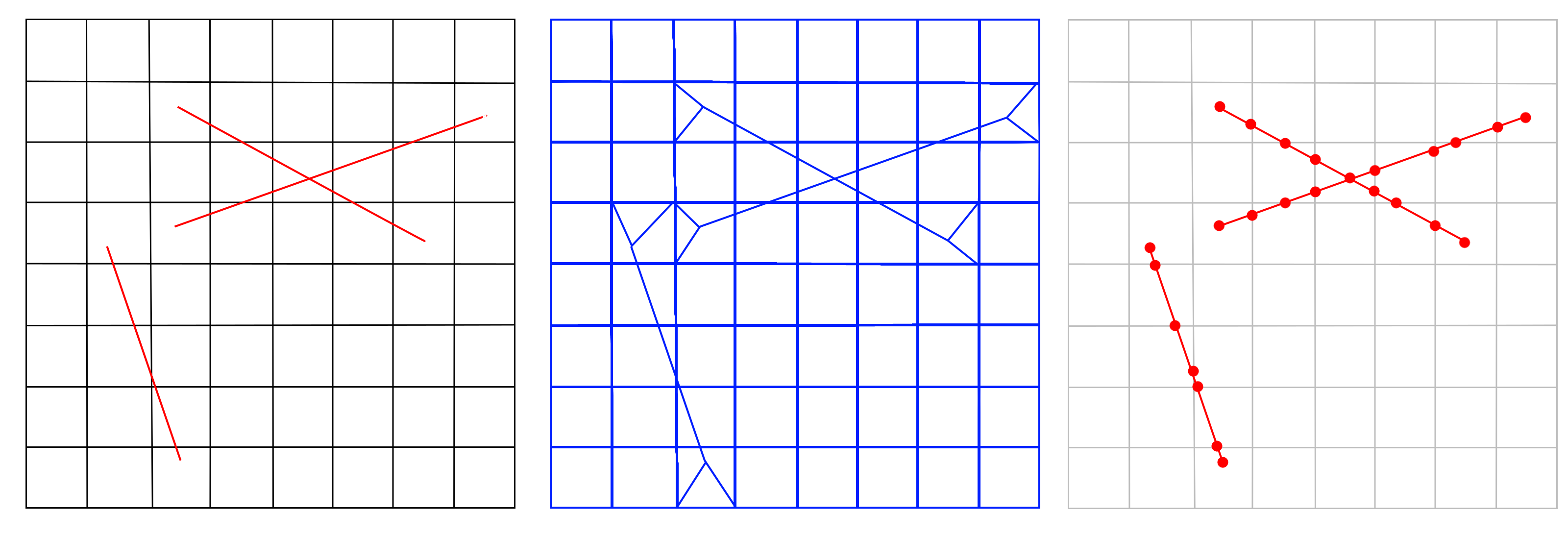
Figure 4: Creation of a polygonal mesh from a regular Cartesian grid.

5.3 Agglomeration

Polytopal grids can be generated by agglomerating simplicial elements produced, for instance, by a constrained Delaunay procedure. For example, in [16], tetrahedra are agglomerated (and nodes moved) to try to produce hexahedral elements in large part of the domain, with a twofold objective: on the one hand the reduction of the total number of degrees of freedom and consequent reduction of computational complexity, on the other hand, the generation of a grid more suitable for finite volume schemes based on two-point flux approximation (TPFA).

In a more general setting, agglomeration may join together elements whose value of physical parameters are similar, with the final objective of reducing computational cost, as well as eliminating excessively small elements. The numerical method, however, should be able to operate properly on the possible irregularly shaped and non-convex elements generated by the procedure. The technique is clearly a post-processing one, since it requires to have a mesh to start with. Its basic implementation is however rather simple and is similar to that used in some multigrid solvers, like in [43].

In our case, PorePy has the capability to agglomerate cells based on two different criteria: (i) by volume, meaning that cells with small volumes are grouped with neighbouring cells. This procedure continues until the new created cells have volumes that are comparable with an averaged volume in the grid. This procedure can be effective in presence of uniform physical data in different part of the computational domain and in particular in presence of fracture networks. In the case of highly variable data, e.g. permeability, the previous procedure may not be effective since cells with very different properties may be merged together. For this reason PorePy implements another strategy, (ii) based on the agglomeration in the algebraic multigrid method. It adopts a measure of the strength of connections between DOFs to select the cells to be joined, based on a two-point flux approximation discretization, for more details see [59, 38]. Examples of these strategies are given in [38, 39, 36, 40, 49].

5.4 Voronoi

Voronoi grids are of particular interest for methods such as Finite Volumes with TPFA, since they guarantee that the line connecting the centroids of neighbouring cells is always orthogonal to the shared face. Under this assumption the two point approximation of the flux is consistent if the permeability tensor is diagonal. However, producing Voronoi diagrams that honour the internal interfaces represented by the fracture is not an easy task, particularly for complex 3D configurations. An attempt in that direction has been performed in [53] and [12].

In this work, limited to 2D cases, we generate Voronoi diagrams that honour the geometry of the fractures and the boundaries of the domain by first creating a Cartesian grid (see Section 5.2) and positioning a seed at the centre of cells not cut by the fractures. Then, we start from the discretization of the fractures induced by the intersection with the background grid, and for each fracture cell we position two seeds on opposite sides of the fracture at a small distance $\delta$ as shown in Figure 5. This will create a Voronoi cell with a face exactly on the fracture. The same technique is used to obtain boundary faces in the desired position. Close to each fracture tip $\bm{x}_{T}$ we position four seeds in $\bm{x}_{T}\pm\delta_{1}\bm{n}\pm\delta_{2}\bm{t}$ where $\bm{n}$ and $\bm{t}$ are the normal and the tangent unit vectors to the fracture and $\delta_{1,2}$ are user defined distances. This ensures that the fracture is honoured up to the tip and has the correct length. Similar strategies are applied at fracture intersections. The position of the seeds and faces close to the intersections is also shown in Figure 5. Note that with this strategy the Voronoi cells far from fractures are rather regular, since they reflect the underlying Cartesian grid.

An advantage of Voronoi grids is that faces are planar and cells are convex by construction. However, an important drawback is that the number of faces per cell can be quite large. Moreover, as pointed out before, the construction of a constrained grid in general realistic configurations is an open problem.

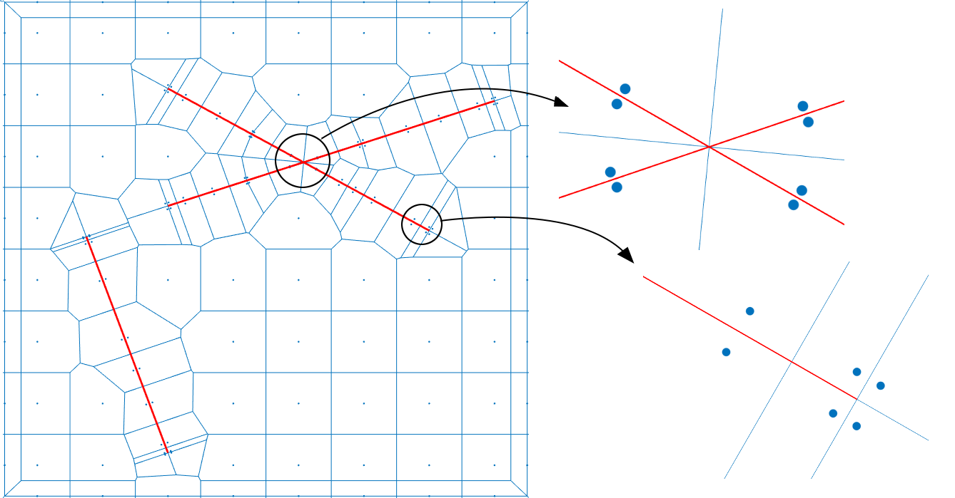
Figure 5: On the left, graphical representation of Voronoi grid with fractures. On the right, details on the construction for fracture intersection and fracture tip.

6 Numerical results

In this section, we present two test cases to show the performances and the potentiality of the previously introduced algorithms. In particular, in the first test case we have a setting where the permeability experiences a high variation between neighbouring cells. In the second test case a network of fractures is considered with different types of intersections: in this case the challenge is more related to the geometrical complexity to create the computational grid. In both test cases, coarsening procedures are used to reduce the computational cost of the simulations.

6.1 Heterogeneous porous medium: layers from SPE10

The aim of this test case is to validate the effectiveness of the MVEM scheme in presence of highly heterogeneous permeability. We consider two distinct layers of the SPE10 [21] benchmark problem, in particular layer 4 and 35 (by starting the numeration from 1), from now on denoted as L4 and L35, respectively. The main difference between them is that the latter has distinctive channels of high permeability which are not present in layer 4. The permeability is assumed to be scalar in each cell, and each layer is composed by a computational grid of $60\times 220$. Figure 6 on the left shows the permeability fields for both layers. Note that in both cases permeability spans about six order of magnitude.

To lighten the computational effort, we apply a coarsening procedure to group cells and obtain a smaller problem. Starting from square cells the algorithm creates cells by considering the procedure in Subsection 5.3 and, for each coarsened cell, the associated permeability will be computed in two different ways: as the arithmetic and harmonic average. The former is more suited for flow parallel to layers of different permeability, while for orthogonal flow the harmonic average gives more realistic results. For a more detailed discussion see [50]. We consider both approaches, see Figure 6 on centre and right, which represents the coarsened permeability of both layers by considering the arithmetic and harmonic means.

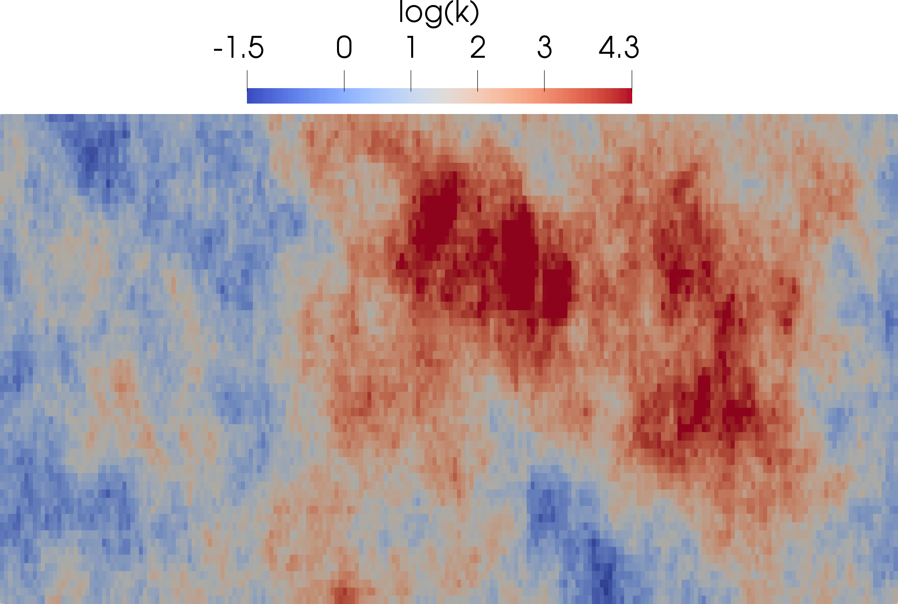
(a) L4 original

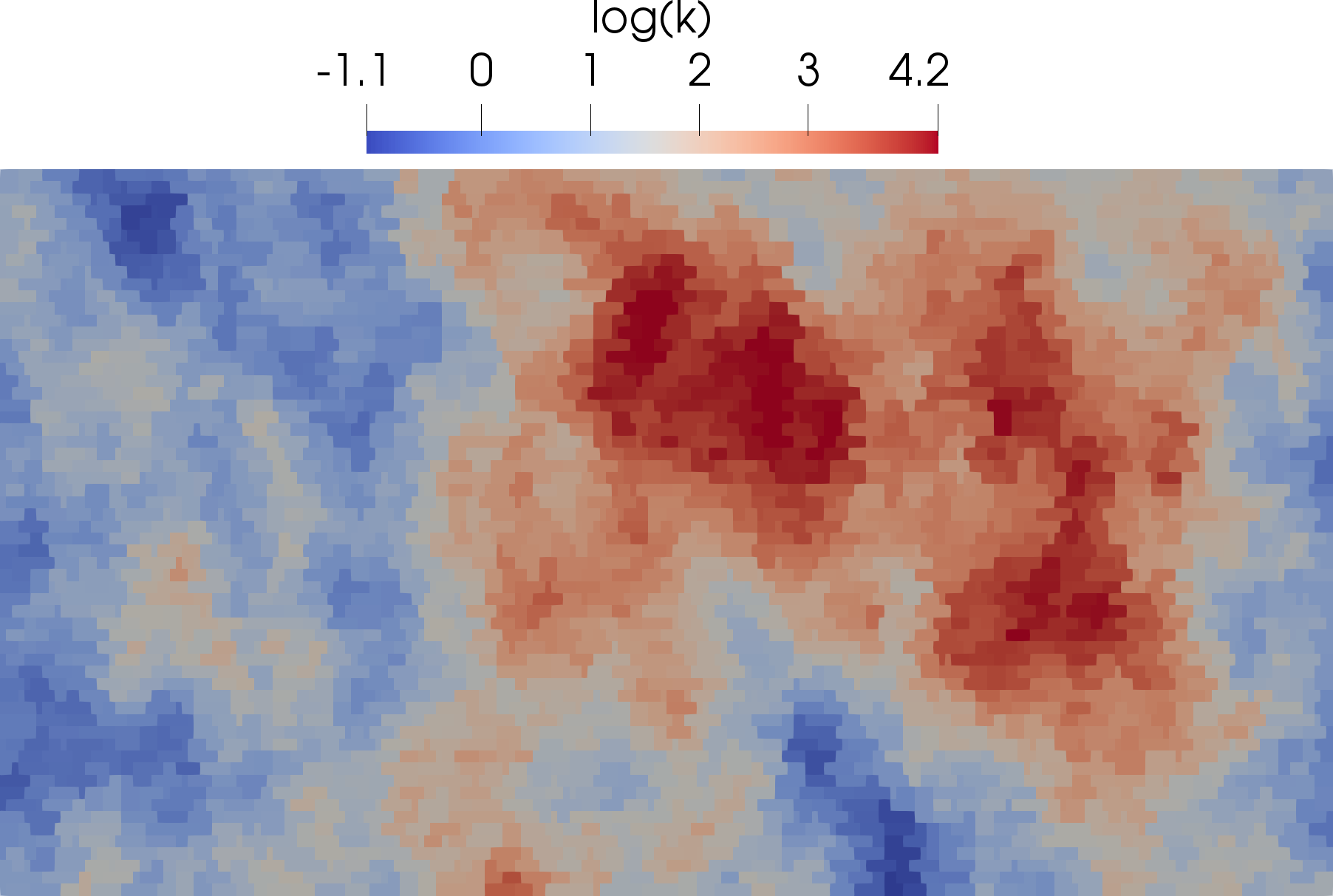
(b) L4 coarsened with arith. mean

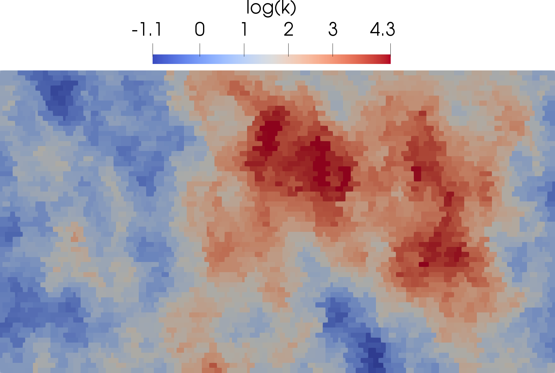
(c) L4 coarsened with harm. mean

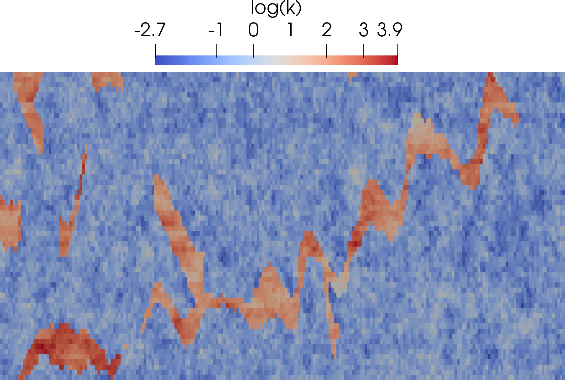
(d) L35 original

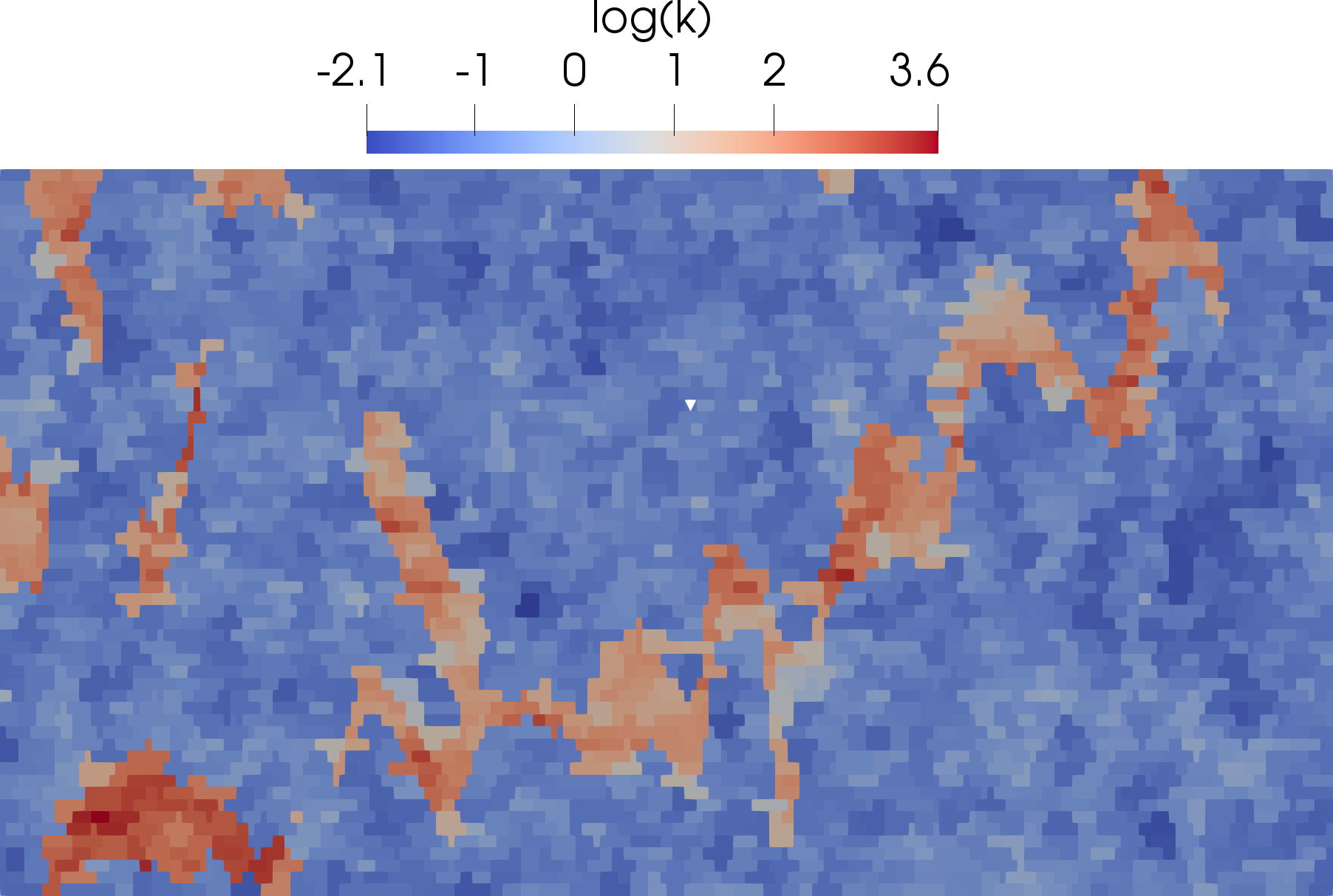
(e) L35 coarsened with arith. mean

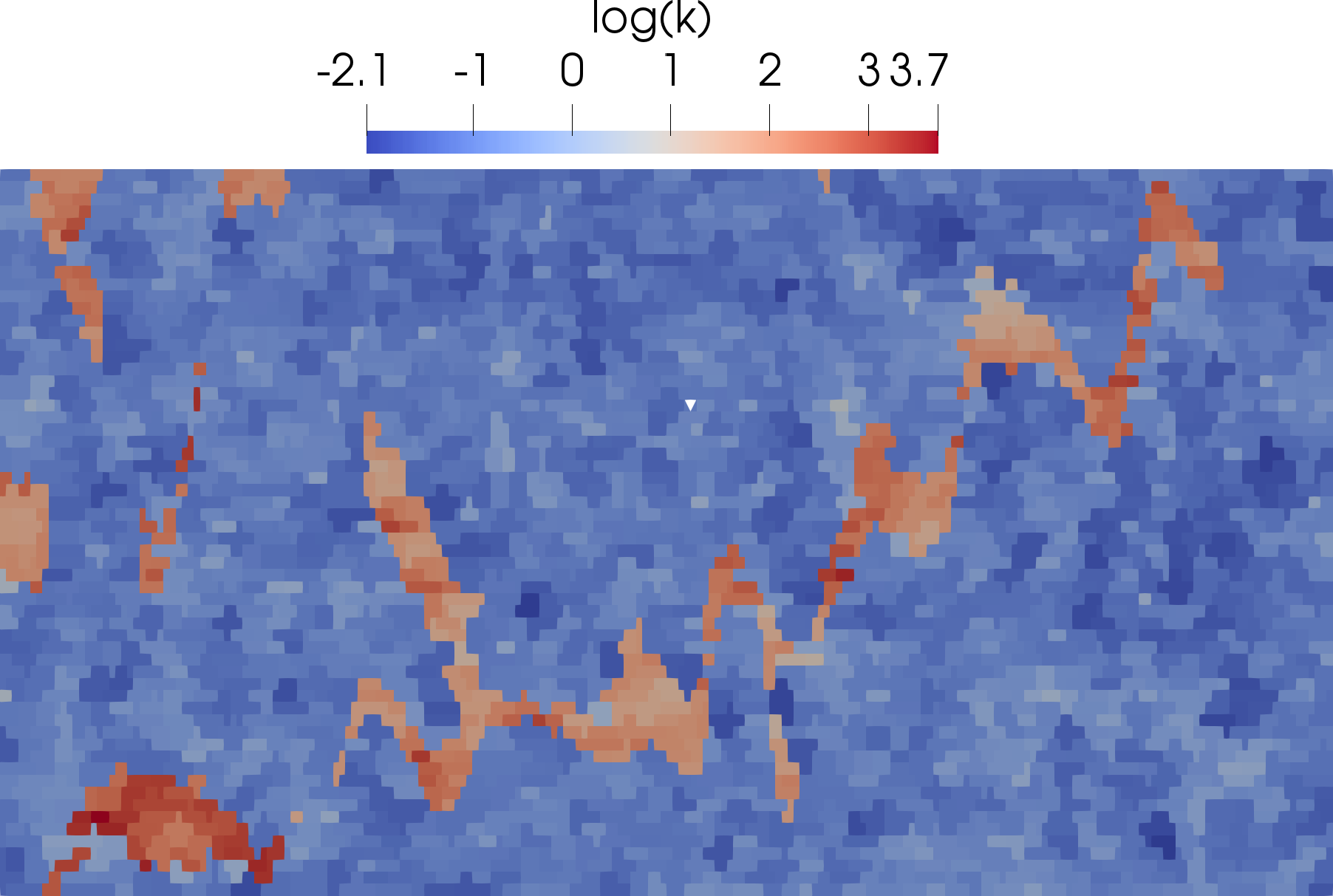
(f) L35 coarsened with harm. mean

Figure 6: Permeability field for the test case of Subsection 6.1 for layer 4 on the top and 35 on the bottom. On the left the reference values, on the centre and right the values obtained after the clustering with arithmetic and harmonic mean, respectively. The values are given in $\log_{10}$.

For layer 4 the figures look similar, while for layer 35 the channels for the coarsened problem with harmonic mean are narrower than the original ones and than those obtained in the coarsened grid with arithmetic mean.

In Table 1, we summarize the geometric properties of the grids obtained by means of cells clustering for the two layers. We can observe that the area of the cells and the average number of faces per cell is similar in the two cases, however, in layer 35 we have slightly more elongated elements on average, reflecting the channelized permeability field. The aspect ratio is estimated using the area of the cells, the maximum distance between points is rescaled so that square cells (or equilateral triangles, see Section 6.2) have aspect ratio 1.

	aspect ratio			cell area			$n_{\mathrm{faces}}$
	average	min	max	average	min	max	average	min	max
L4	2.37	1.50	4.37	108	37.2	242	12.2	6	20
L35	2.37	1.13	5.83	111	37.2	297	12.2	6	22

Table 1: Average, minimum and maximum value of cell area and number of faces per cell for the six grids employed for Test case 6.1

We impose a pressure gradient from left to right with synthetic values 1 and 0, respectively. The other boundaries are sealed with homogeneous Neumann conditions.

To compare the accuracy of the proposed clustering techniques, we compute the errors in the pressure with respect to the problem on the original grid solved with a two-point flux approximation scheme [2, 35], which, in this case since the grid is $K$-orthogonal, is consistent and converges quadratically to the exact solution, thus can be considered as a valid reference. We name this solution “reference” and we indicate the pressure as $p_{\rm ref}$. The error is computed as

$$err=\frac{{\left\|{\Pi_{\rm ref}p-p_{\rm ref}}\right\|}_{L^{2}(\Omega)}}{{\left\|{p_{\rm ref}}\right\|}_{L^{2}(\Omega)}}$$

where $\Pi_{\rm ref}$ is the piecewise constant projection operator that maps from the current grid to the reference one. Due to the clustering procedure its construction is rather straightforward, since the cells of the original mesh are nested in the coarsened one. We can notice that the errors obtained for the layer 4 with both averaging procedure are comparable and around $4\%$, which can be acceptable in most of real applications. In the case of layer 35 the situation is more involved, in fact the arithmetic mean gives an error of approximately $3.5\%$ while the harmonic mean of $13\%$. We can explain this big discrepancy by noticing that, when a channel of high permeability is composed by few cells in its normal direction, during the coarsening procedure it is possible that some of these cells are grouped with the surrounding lower permeability cells. The harmonic mean will bring the permeability value of the coarsened cell closer to the lower value than the higher, dramatically changing the connectivity properties of the obtained permeability field. This can be noticed in the permeability field reported in Figure 6, suggesting that harmonic averaging can be unsuited for parallel flow in strongly channeled domains.

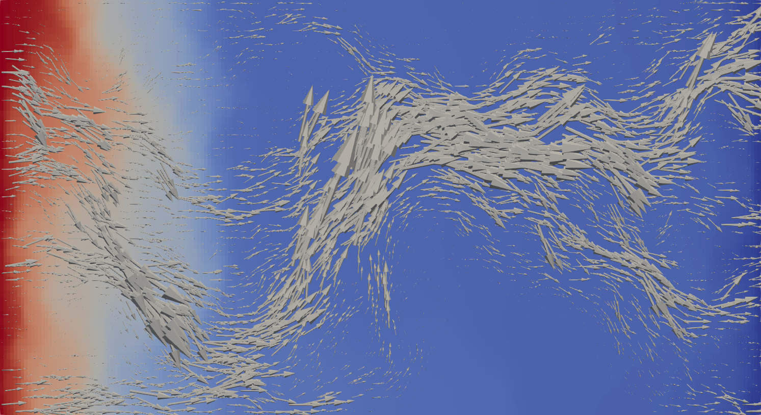
(a) L4 original

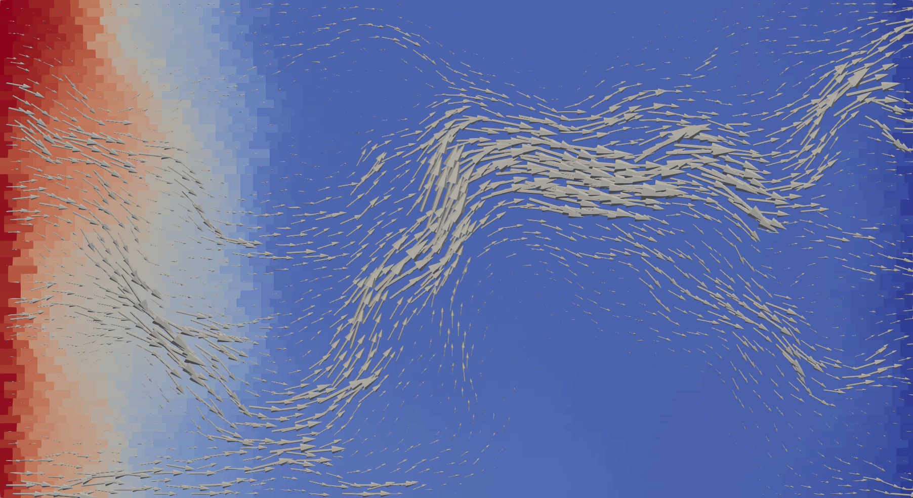
(b) L4 coarsened with arith. mean

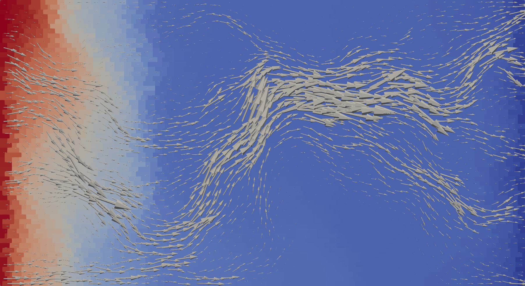
(c) L4 coarsened with harm. mean

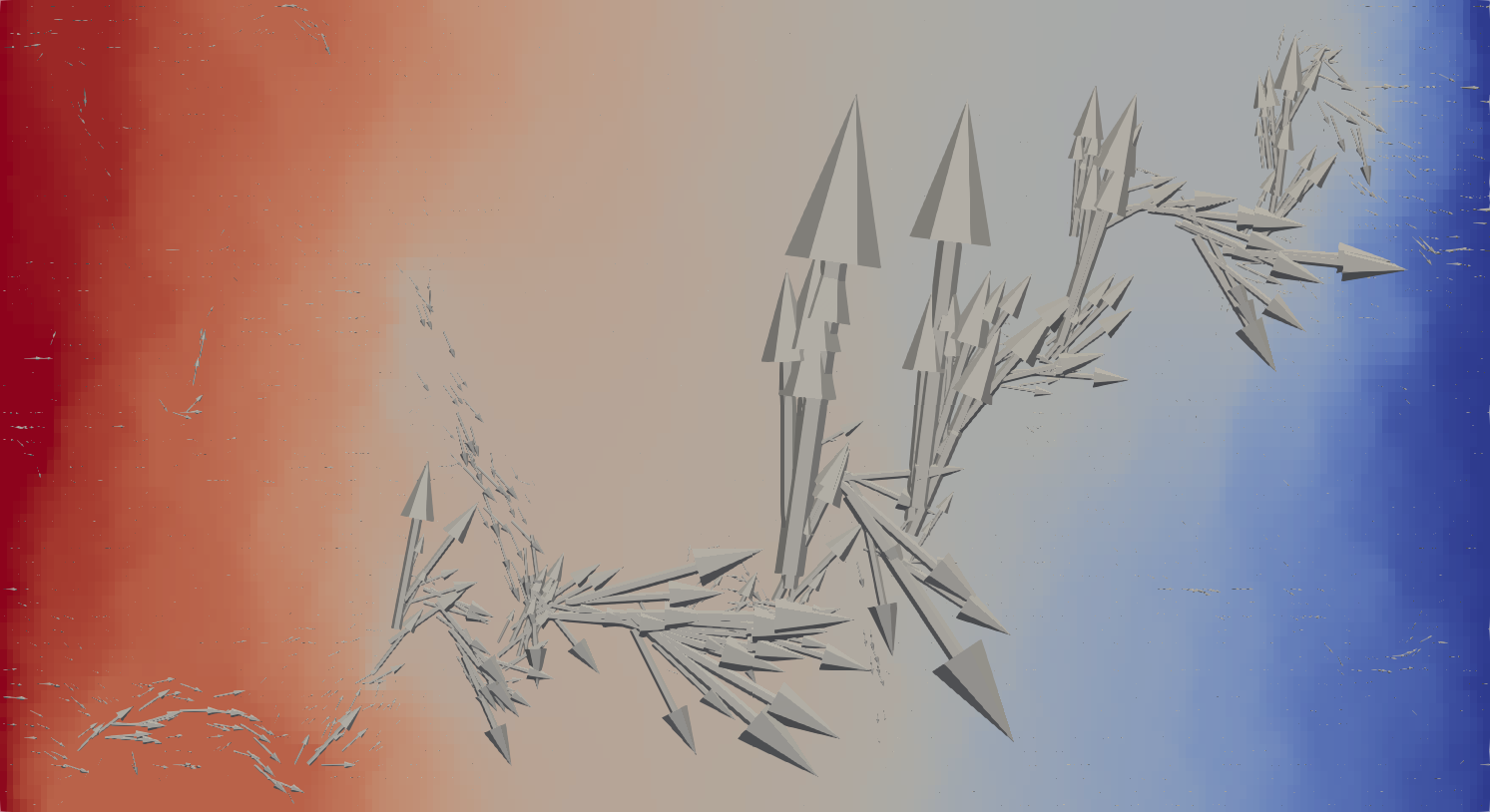
(d) L35 original

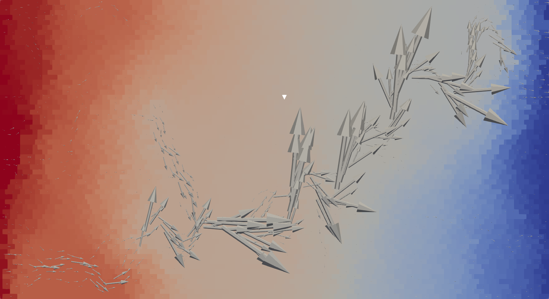
(e) L35 coarsened with arith. mean

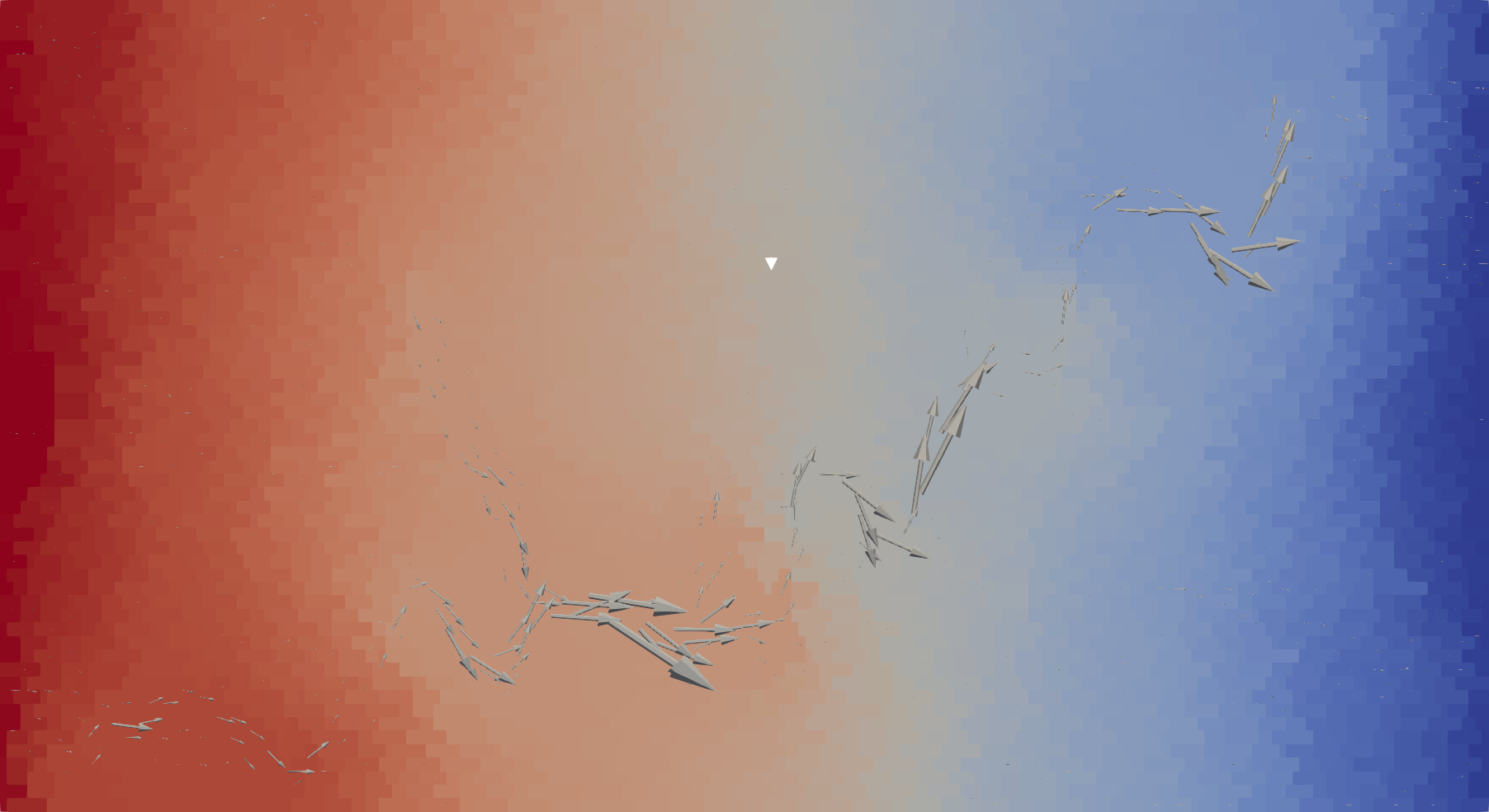
(f) L35 coarsened with harm. mean

Figure 7: Pressure and Darcy velocity fields for the test case of Subsection 6.1 for layer 4 on the top and 36 on the bottom. On the left the reference solution, on the center and right the values obtained after the clustering with arithmetic and harmonic mean, respectively. The arrows are scaled by the same value in each layer and the pressure ranges from 0 to 1, blue to red respectively.

Figure 7 shows the pressure fields for both layers and for the two approaches. On top of the pressure fields the Darcy velocity is also represented with grey arrows. We notice that for layer 4 pressures and velocities look very similar, while for layer 35 the pressure field and velocity of the coarsened problem with harmonic mean look quite different compared with the reference solutions as well as that obtained with the coarsened strategy that uses the arithmetic mean.

To improve the effectiveness of this approach, a local numerical upscaling technique could be considered to compute a more representative value of the permeability for grouped cells. However, in this case we might expect a higher computational cost. See [27] for a more detailed presentation of upscaling techniques.

To conclude this test case, let us now analyze the properties of the system matrix to verify what is the impact of element size and shape in the different cases. Note that the problem is in mixed form and our analysis considers the entire saddle point matrix. Since the number of unknowns is not exactly the same after grid agglomeration we describe matrix sparsity by means of the average number of non-zero entries per row $\overline{n}$, computed as

$$\overline{n}=\frac{n_{z}}{N_{\mathrm{DOF}}},$$

where $n_{z}$ is the number of non-zero entries and $N_{\mathrm{DOF}}$ is the number of unknowns. Moreover we will compare the values of condition number $K(A)$ estimated by the method condest provided by Matlab^®. In Table 2 we consider the two layers, L4 and L35, and by “mean K”, “harmonic K” we identify the averaging of permeability in the coarse cells, the arithmetic and harmonic mean respectively. This choice has no impact on the matrix size or sparsity but may result in different condition numbers. We can observe that the four matrices are very similar in terms of size, sparsity and condition number, and that the large number of faces per element reflects in the average number of entries per row. It can be also observed that mesh coarsening is slightly more effective in layer L35 due to its channelized permeability distribution.

	$N_{\mathrm{DOF}}$	$N_{\mathrm{cells}}$	$N_{\mathrm{faces}}$	$\overline{n}$	$K(A)$
L4 (mean K)	16345	2269	14076	22.17	8.29e+06
L4 (harmonic K)	16345	2269	14076	22.17	8.44e+06
L35 (mean K)	16010	2210	13800	22.53	8.29e+06
L35 (harmonic K)	16010	2210	13800	22.53	8.39e+06

Table 2: Matrix properties for Test case 6.1

6.2 Fracture network

This test case considers the Benchmark 3 of the study [28] presented in Subsection 4.3. Our objective is to study the impact of the grid on the solution quality provided by the MVEM. The domain contains a fracture network made of 10 fractures and 6 intersections, one of which is of $L$-shape. For the detailed fracture geometry, we refer to the aforementioned work. See Figure 8 for a representation of the problem geometry.

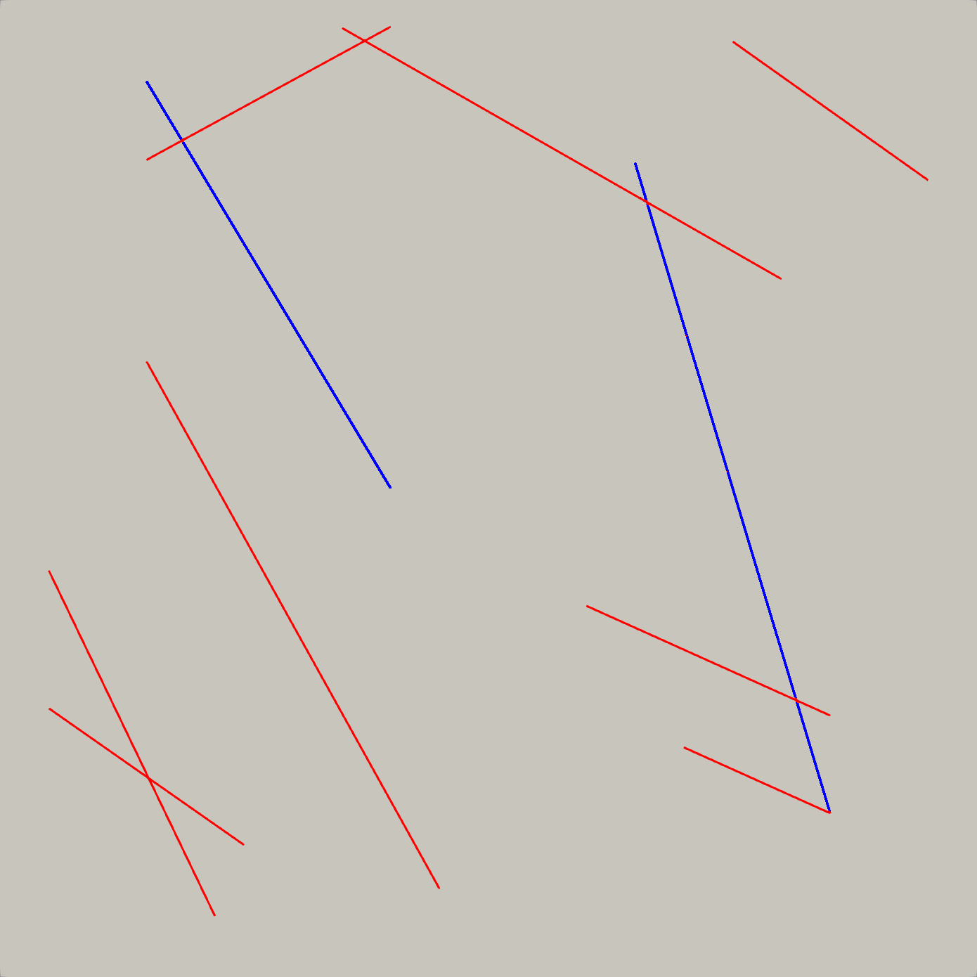
Figure 8: Geometry of the domain for the benchmark used in Subsection 6.2.

We consider three types of grids: Delaunay, Cartesian cut, and Voronoi. Since the fracture network may create small cells, on top of these three grids a coarsening algorithm is used to agglomerate cells of small volume. These cells are merged with neighbouring cells, trying to obtain a more uniform cell size in the grid. The Delaunay grid is created by the software Gmsh [42], tuned to provide high quality elements in proximity of small fracture branches or almost intersecting fractures. The six different grids we are considering are reported in Figure 9 along with the number of cells associated to the rock matrix and fractures.

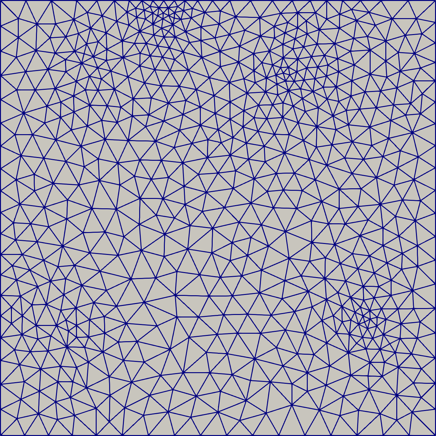
(a) Delaunay (1275, 276)

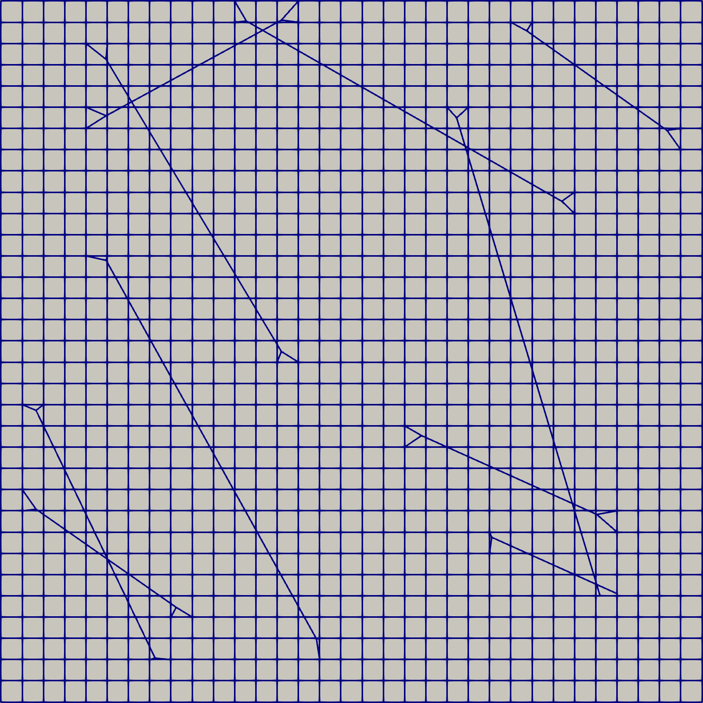
(b) Cartesian cut (1296, 579)

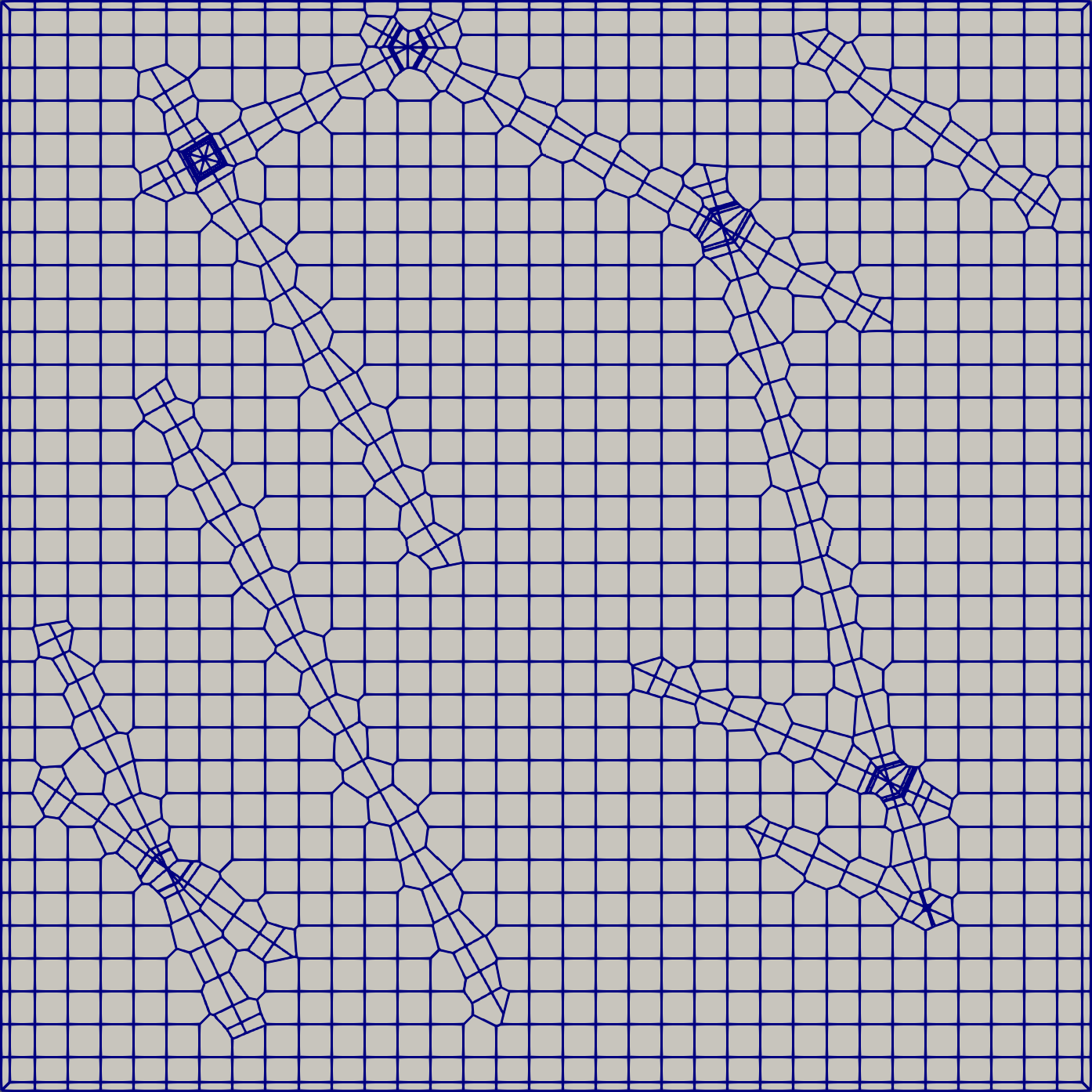
(c) Voronoi (1521, 633)

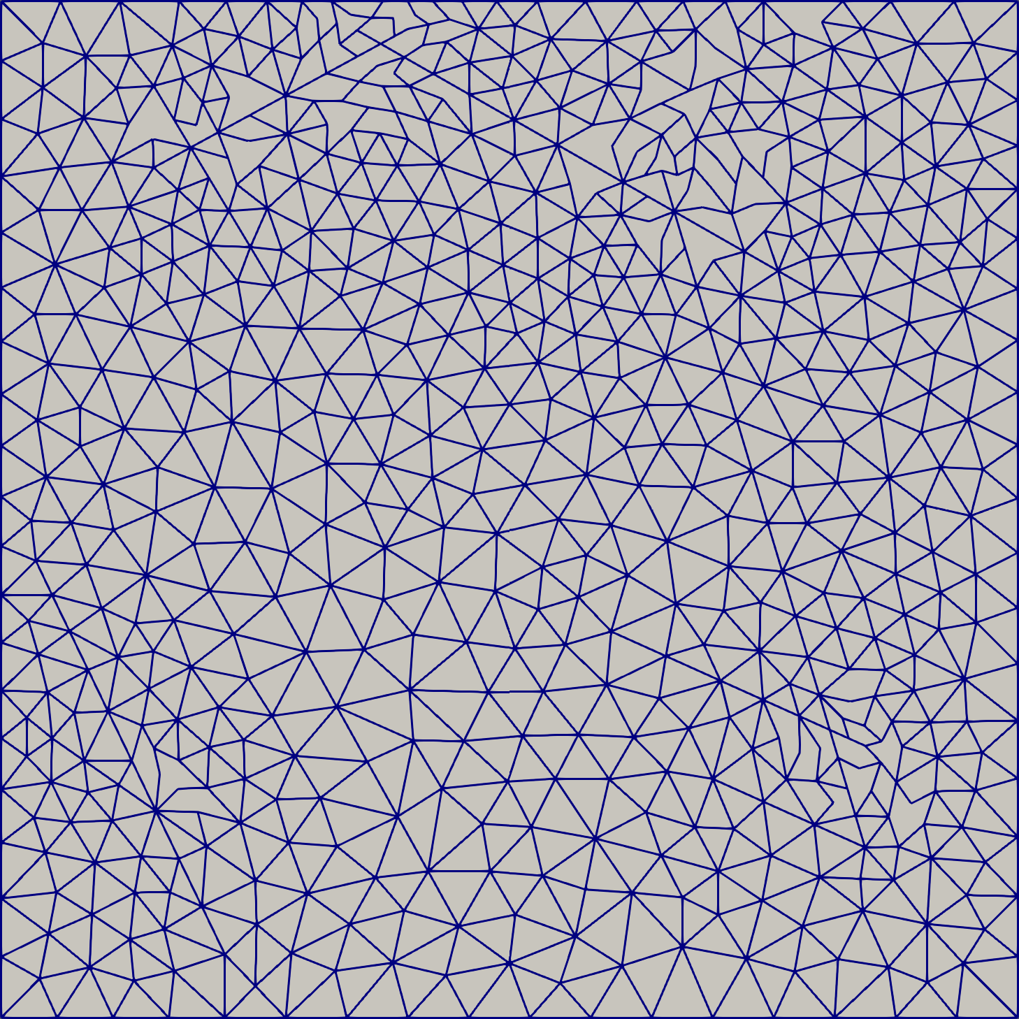
(d) Delaunay coarse (1098, 276)

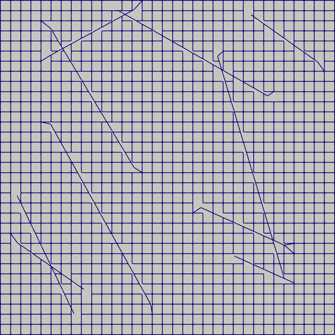
(e) Cartesian cut coarse (1053, 579)

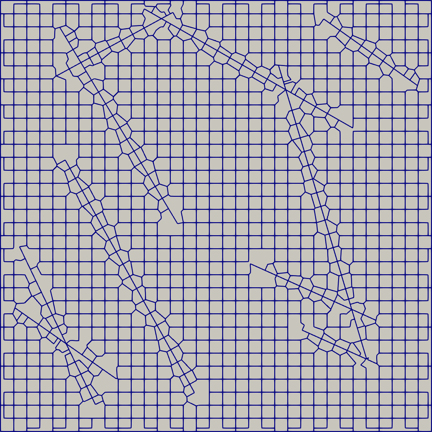
(f) Voronoi coarse (1109, 633)

Figure 9: Benchmark 3 of Subsection 6.2: Fracture network on top left, on the others the grids for different approaches. In the brackets the number of cells (bulk, fracture).

We see that some of the agglomerated elements have internal cuts, in particular for Figure 9d, and for all the clustered grids we have cells that are not shape regular and in some cases not even star-shaped. For classical finite elements or finite volumes we might expect low quality results.

Another result of the coarsening is a reduction of the number of very small or very stretched cells. In Figure 10 we can observe histograms of an estimate of the cells aspect ratio for the different grids. We can see that for the Cartesian cut grid and the Voronoi grid the maximum aspect ratio decreases remarkably with the agglomeration, while in the case of a Delaunay grid we have the opposite effect. As we will show later high anisotropy can result in a less effective stabilization for the MVEM matrix. Moreover, in Table 3 we show that cells agglomeration leads to an increase of the mean and minimum cell areas, but also to an increase of the number of faces per cell.

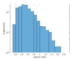
(a) Delaunay

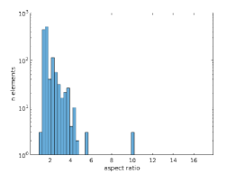
(b) Cartesian cut

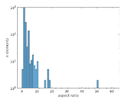
(c) Voronoi

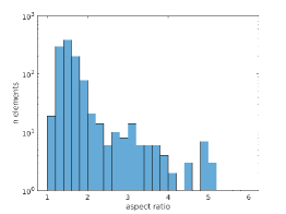
(d) Delaunay coarse

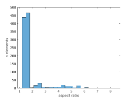
(e) Cartesian cut coarse

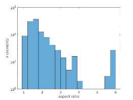
(f) Voronoi coarse

Figure 10: Histograms of the cells aspect ratio for the different types of grid in test case 6.2.

	cell area			$n_{\mathrm{faces}}$
	average	min	max	average	min	max
Delaunay	7.8431e-04	8.4186e-05	2.1020e-03	3	3	3
Delaunay coarse	9.1075e-04	3.9631e-04	2.1767e-03	3.1557	3	8
Cut	7.7160e-04	8.4664e-08	9.1833e-04	3.9769	3	6
Cut coarse	9.4967e-04	3.9945e-04	2.2589e-03	4.4311	3	10
Voronoi	6.5746e-04	4.6260e-07	1.2686e-03	4.4694	3	14
Voronoi coarse	9.0171e-04	3.3000e-04	3.4502e-03	5.1109	4	16

Table 3: Average, minimum and maximum value of cell area and number of faces per cell for the six grids employed for test case 6.2

Referring to the colour code given in Figure 8, we set the aperture $\epsilon=10^{-4}$ for all the fractures and the permeability is set to $k_{\gamma}=\kappa_{\gamma}=10^{4}$ for all the fractures depicted in red and $k_{\gamma}=\kappa_{\gamma}=10^{-4}$ for the ones in blue. The former behave as high flow channels while the latter as low permeable barriers. The rock matrix is characterized by a unit scalar permeability. In [28] two sets of boundary conditions were considered, left-to-right and bottom-to-top. In our case we choose the former, meaning that we set a value of pressure equal to 4 on the left side of $\Omega$ and to 1 on the right side of $\Omega$. The other two boundaries are considered as impervious.

In Figure 11a we report the plot of pressure over the line $(0,0.5)-(1,0.9)$, by using the grids shown in Figure 9.

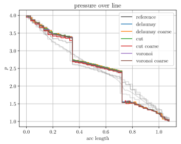
(a) Pressure over line $(0,0.5)-(1,0.9)$

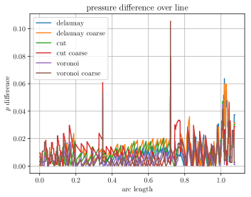
(b) Pressure difference over line $(0,0.5)-(1,0.9)$

Figure 11: On the left, pressure over line for the test case of 6.2. The grey solutions are the one reported in [28]. Most of the plots overlap with the reference solution, in black. On the right, the difference over the same line between a solution and the reference one.

In light grey we present the results obtained in the benchmark [28] and in black the reference solution. We clearly see that all the proposed methods overlap with the reference solution showing high accuracy even on such coarse grids. In particular results do not deteriorate with the coarsening procedure. Moreover, comparing with the results obtained in [28] the ones given by the MVEM are, generally, of higher quality.

In Figure 11b, we show the pressure difference between the reference solution and the ones obtained with the considered grids, over the reference solution itself. The errors are quite small except for the two peaks in correspondence of the pressure jump of Figure 11a. The reason can be associated to the sampling procedure used in the extraction of these data.

Finally, as done in [28] we compute the errors in the rock matrix between the reference and the computed solution. We consider the following formula

$$err_{m}^{2}=\frac{1}{{\left|{\Omega}\right|}(\Delta p_{ref})^{2}}\sum_{f=K_{m}\cap K_{ref,m}}{\left|{f}\right|}\left(p_{m}|_{K_{m}}-p_{ref}|_{K_{ref,m}}\right)^{2},$$ (8)

where $p_{m}|_{K_{m}}$ is the pressure of the $m$-method at cell $K_{m}$, $p_{ref}$ is the reference pressure at cell $K_{ref,m}$, and $\Delta p_{ref}$ is the maximum variation of the pressure on all the domain. These errors are reported in Table 4.

	original	coarsened
Delaunay	0.013008	0.014267
Cartesian cut	0.012865	0.025827
Voronoi	0.0085291	0.010037

Table 4: Pressure error between the reference solution and the compute with the MVEM by using formula 8.

All the errors are quite small and comparable with those reported in [28]. When the coarsening procedure is adopted, the errors slightly increase due to the smaller number of cells except for the Cartesian cut case where the error doubles, remaining nevertheless acceptable.

Let us now analyze the properties of the system matrix to verify what is the impact of element size and shape in the different cases. We remind that the grids have been generated with comparable resolution to obtain similar numbers of degrees of freedom, however, the number of unknowns is not exactly the same. Results are summarized in Table 5. From the point of view of the degrees of freedom the Voronoi grid is the most demanding because, for a given space resolution it generates very small cells close to the intersections and tips, however, it is also the one that benefits the most from coarsening. The conditioning is of the same order of magnitude for all grids, and improves with coarsening. In particular the best result is obtained for the coarsened Voronoi grid despite the large number of faces per element that results from clustering of general polygons and reflects in the slightly larger number of non-zero entries per row.

	$N_{\mathrm{DOF}}$	$N_{\mathrm{cells}}$	$N_{\mathrm{faces}}$	$\overline{n}$	$K(A)$
Delaunay	3741	1373	2162	5.15	4.82E+10
Delaunay coarse	3384	1196	1982	5.51	3.85E+10
Cut	4961	1495	1296	6.00	4.23E+10
Cut coarse	4474	1252	2814	7.42	3.67E+10
Voronoi	6095	1738	3913	7.33	4.10E+10
Voronoi coarse	5118	1326	3348	9.32	3.21E+10

Table 5: Matrix properties for Test case 6.2

We can also observe that, even if the sparsity of the matrices is similar in all cases, the pattern can change significantly. In Figure 12 we compare the matrix structure corresponding to a Delaunay grid and a Cartesian cut one: the underlying structure of the Cartesian grid has a visible impact on the sparsity pattern. A similar structure is observed for the case of the Voronoi grid since, away from the fracture network, the seeds are positioned to obtain a Cartesian grid. Let $T_{\alpha}$ denote the time required to solve 1000 times the system arising from the discretization on a mesh $\alpha$ with the ”$\backslash$” method from Matlab^®, and let $\tilde{T}_{\alpha}=\frac{T_{\alpha}}{(N_{\mathrm{DOF}}^{\alpha})^{3}}$ be the time normalized against the third power of the system size. The corresponding values, reported in Table 6, seem to indicate that, for the same sparsity, a faster solution is obtained with a more compact pattern. Solution strategies for this kind of problem can be found in [24].

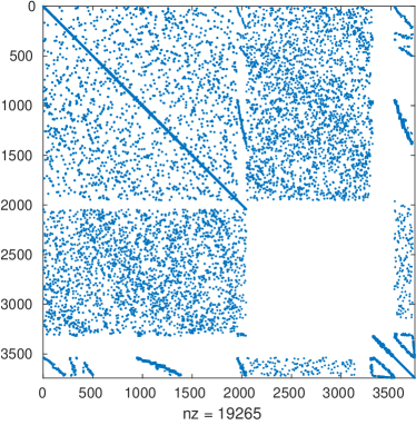
(a) Delaunay grid

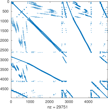
(b) Cartesian cut grid

Figure 12: The sparsity patterns for a Delaunay grid (left) and the Cartesian cut grid (right).

	Delaunay	Delaunay coarse	Cut	Cut coarse	Voronoi	Voronoi coarse
$\tilde{T}_{\alpha}$	2.630e-10	3.410e-10	1.889-e10	2.262e-10	1.394e-10	2.246e-10

Table 6: Normalized time for the solution of the linear systems corresponding to the different grids.

Finally, we study the effect of element shape on the MVEM stabilization term. We define element-wise an index

$$\kappa_{i}=\frac{||S_{i}||}{||S_{i}||+||A_{i}||}$$

where $S_{i}$ and $A_{i}$ are the local stability and consistency contributions to the matrix arising from the discretization of the bilinear form $a_{\Omega}$ on the $i-$th element.

As shown in Figure 13 in the case of a Delaunay grid the norm of the stabilization term in each local matrix is comparable to the norm of the consistency term, i.e. $\kappa_{i}\simeq 0.5$ everywhere. In the Voronoi grid instead we have elements with extremely high aspect ratios (up to 60), or, in other words, we have small edges compared to the typical mesh size. In this latter case the norm of the stability term is one order of magnitude smaller in elements with very small edges. A discussion of the stability bounds for grids in the case of small edges can be found in [8], [9] for the primal formulation of elliptic problems.

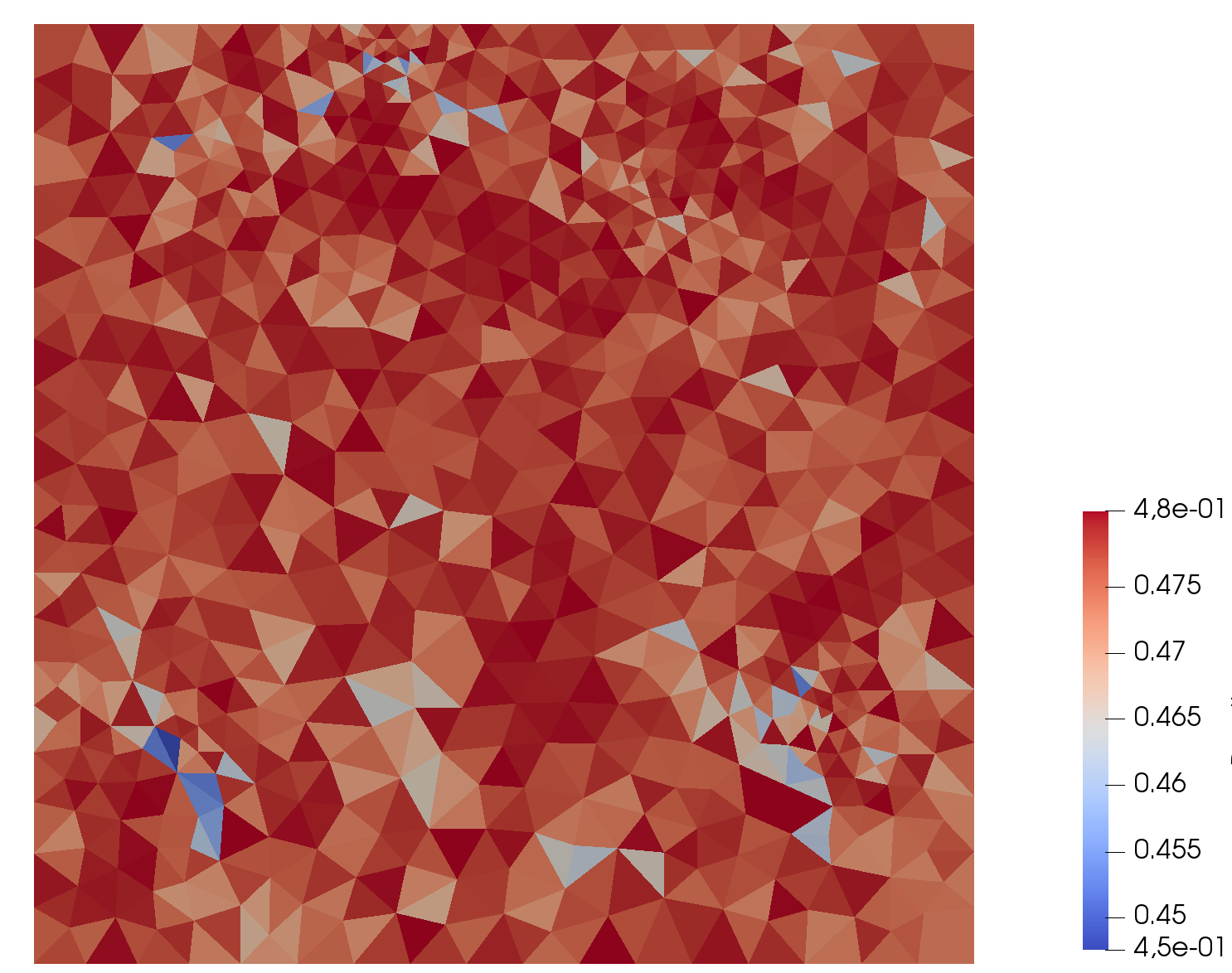
(a) Delaunay grid

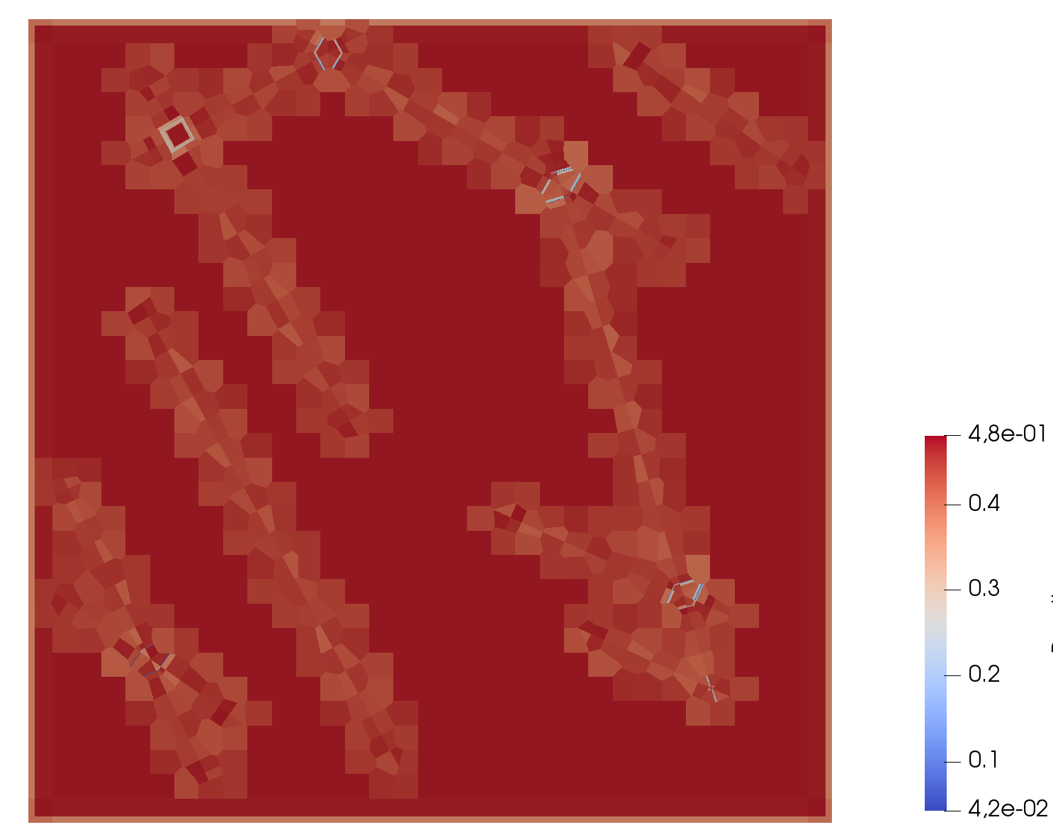
(b) Voronoi grid

Figure 13: On the left, $\kappa_{i}$ on the Delaunay grid, on the right the same index on the Voronoi grid before clustering.

7 Conclusion

In this work we have presented and discussed the performances of the Mixed Virtual Finite Element Method applied to underground problems. One of its main advantages is the possibility to handle, in a natural way, grid cells of any shape becoming suitable for its usage in problems with complex geometries, such as subsurface flows. A second strong point is the ability of the scheme to handle, in a robust way, strong variations of the permeability matrix which is again a common aspect for underground processes. Finally, the numerical scheme is also locally mass conservative making it very suitable in the coupling of other physical processes, like transport problems. We have tested the capabilities of the scheme with respect to two test cases that are known in literature and stress the two aforementioned critical points: heterogeneity and geometrical complexity. A first remark is that the mixed virtual element method gives high quality results also for challenging grids and physical data, making it a promising and interesting scheme for industrial applications. Moreover we performed some comparisons of the system matrices arising from the discretization of the problem on different types of grids: Delaunay, Voronoi, Cartesian grids cut by fractures. We observed similar condition numbers and sparsity, but a better sparsity patterns for grids obtained from the modification of structured ones. We also applied coarsening by means of permeability based and volume based clustering: besides reducing the computational cost this technique allowed us to eliminate small cells and, in some cases, cells with very large aspect ratios where the MVEM stabilizazion term employed in this work does not scale correctly. Future research may focus on the choice of the most stabilization term formulation for the grid type, as well as to the generalization of this work to the three dimensional case, including the discussion of corner point grid which are widely used in subsurface flows but pose many challenges due to the presence of non-planar faces and non-convex elements.

8 Acknowledgements

We acknowledge the PorePy development team: Eirik Keilegavlen, Runar Berge, Michele Starnoni, Ivar Stefansson, Jhabriel Varela, Inga Berre.

References

- [1] The Computational Geometry Algorithms Library. http://www.cgal.org.
- [2] Ivar Aavatsmark. Interpretation of a two-point flux stencil for skew parallelogram grids. Computational Geosciences, 11(3):199–206, 2007.
- [3] Clarisse Alboin, Jérôme Jaffré, Jean E. Roberts, and Christophe Serres. Modeling fractures as interfaces for flow and transport in porous media. In Fluid flow and transport in porous media: mathematical and numerical treatment (South Hadley, MA, 2001), volume 295 of Contemp. Math., pages 13–24. Amer. Math. Soc., Providence, RI, 2002.
- [4] Paola Francesca Antonietti, Luca Formaggia, Anna Scotti, Marco Verani, and Nicola Verzotti. Mimetic finite difference approximation of flows in fractured porous media. ESAIM: M2AN, 50(3):809–832, 2016.
- [5] Jacob Bear. Dynamics of Fluids in Porous Media. American Elsevier, 1972.
- [6] Lourenço Beirão da Veiga, Franco Brezzi, Luisa Donatella Marini, and Alessandro Russo. H(div) and H(curl)-conforming VEM. Numerische Mathematik, 133(2):303–332, Jun 2014.
- [7] Lourenço Beirão da Veiga, Franco Brezzi, Luisa Donatella Marini, and Alessandro Russo. The hitchhiker’s guide to the virtual element method. Mathematical Models and Methods in Applied Sciences, 24(08):1541–1573, 2014.
- [8] Lourenço Beirão da Veiga, Franco Brezzi, Luisa Donatella Marini, and Alessandro Russo. Mixed virtual element methods for general second order elliptic problems on polygonal meshes. ESAIM: M2AN, 50(3):727–747, 2016.
- [9] Lourenço Beirão da Veiga, Carlo Lovadina, , and Alessandro Russo. Stability analysis for the virtual element method. Mathematical Models and Methods in Applied Sciences, 27(13):2557–2594, 2017.
- [10] Matías Fernando Benedetto, Stefano Berrone, Andrea Borio, Sandra Pieraccini, and Stefano Scialò. A hybrid mortar virtual element method for discrete fracture network simulations. Journal of Computational Physics, 306:148 – 166, 2016.
- [11] Matías Fernando Benedetto, Stefano Berrone, Sandra Pieraccini, and Stefano Scialò. The virtual element method for discrete fracture network simulations. Computer Methods in Applied Mechanics and Engineering, 280(0):135–156, 2014.
- [12] Runar Lie Berge, Øystein Strengehagen Klemetsdal, and Knut-Andreas Lie. Unstructured Voronoi grids conforming to lower dimensional objects. Computational Geosciences, 23(1):169–188, 2019.
- [13] Inga Berre, Florian Doster, and Eirik Keilegavlen. Flow in fractured porous media: A review of conceptual models and discretization approaches. Transport in Porous Media, 130(1):215–236, 2019.
- [14] Daniele Boffi, Franco Brezzi, and Michel Fortin. Mixed Finite Element Methods and Applications. Springer Series in Computational Mathematics. Springer Berlin Heidelberg, 2013.
- [15] Wietse M. Boon, Jan M. Nordbotten, and Ivan Yotov. Robust discretization of flow in fractured porous media. SIAM Journal on Numerical Analysis, 56(4):2203–2233, 2018.
- [16] Arnaud Botella, Bruno Lévy, and Guillaume Caumon. Indirect unstructured hex-dominant mesh generation using tetrahedra recombination. Computational Geosciences, 20(3):437–451, apr 2015.
- [17] Konstantin Brenner, Julian Hennicker, Roland Masson, and Pierre Samier. Gradient discretization of hybrid-dimensional Darcy flow in fractured porous media with discontinuous pressures at matrix-fracture interfaces. IMA Journal of Numerical Analysis, September 2016.
- [18] Franco Brezzi, Richard S. Falk, and Donatella Luisa Marini. Basic principles of mixed virtual element methods. ESAIM: M2AN, 48(4):1227–1240, 2014.
- [19] Florent Chave, Daniele A. Di Pietro, and Luca Formaggia. A hybrid high-order method for darcy flows in fractured porous media. SIAM Journal on Scientific Computing, 40(2):A1063–A1094, 2018.
- [20] Siu-Wing Cheng, Tamal K. Dey, and Jonathan Shewchuk. Delaunay Mesh Generation. Chapman and Hall/CRC, 2012.
- [21] Michael A. Christie and Martin J. Blunt. SPE-66599-MS, chapter Tenth SPE Comparative Solution Project: A Comparison of Upscaling Techniques, page 13. Society of Petroleum Engineers, Houston, Texas, 2001.
- [22] Carlo D’Angelo and Anna Scotti. A mixed finite element method for Darcy flow in fractured porous media with non-matching grids. Mathematical Modelling and Numerical Analysis, 46(02):465–489, 2012.
- [23] Fanco Dassi and Giuseppe Vacca. Bricks for the mixed high-order virtual element method: Projectors and differential operators. Applied Numerical Mathematics, 2019.
- [24] Franco Dassi and Simone Scacchi. Parallel solvers for virtual element discretizations of elliptic equations in mixed form. Computers & Mathematics with Applications, 2019.
- [25] Marco Del Pra, Alessio Fumagalli, and Anna Scotti. Well posedness of fully coupled fracture/bulk darcy flow with xfem. SIAM Journal on Numerical Analysis, 55(2):785–811, 2017.
- [26] Jérôme Droniou. Finite volume scheme for diffusion equations: Introduction to and review of modern methods. April 2013.
- [27] Louis J. Durlofsky. Upscaling of geocellular models for reservoir flow simulation: a review of recent progress. In 7th International Forum on Reservoir Simulation Bühl/Baden-Baden, Germany, pages 23–27, 2003. 2003.
- [28] Bernd Flemisch, Inga Berre, Wietse Boon, Alessio Fumagalli, Nicolas Schwenck, Anna Scotti, Ivar Stefansson, and Alexandru Tatomir. Benchmarks for single-phase flow in fractured porous media. Advances in Water Resources, 111:239–258, Januray 2018.
- [29] Bernd Flemisch, Alessio Fumagalli, and Anna Scotti. A Review of the XFEM-Based Approximation of Flow in Fractured Porous Media, volume 12 of SEMA SIMAI Springer Series, chapter Advances in Discretization Methods, pages 47–76. Springer International Publishing, Cham, 2016.
- [30] Luca Formaggia, Alessio Fumagalli, Anna Scotti, and Paolo Ruffo. A reduced model for Darcy’s problem in networks of fractures. ESAIM: Mathematical Modelling and Numerical Analysis, 48:1089–1116, 7 2014.
- [31] Luca Formaggia, Anna Scotti, and Federica Sottocasa. Analysis of a mimetic finite difference approximation of flows in fractured porous media. ESAIM: M2AN, 52(2):595–630, 2018.
- [32] Pascal Frey and Paul Luis George. Mesh Generation. Application to Finite Elements. John Wiley & Sons, 2013.
- [33] Pascal J. Frey, Houman Borouchaki, and Paul-Luis George. 3D Delaunay mesh generation coupled with an advancing-front approach. Computer Methods in Applied Mechanics and Engineering, 157(1-2):115–131, apr 1998.
- [34] Najla Frih, Vincent Martin, Jean Elisabeth Roberts, and Ai Saâda. Modeling fractures as interfaces with nonmatching grids. Computational Geosciences, 16(4):1043–1060, 2012.
- [35] Helmer André. Friis, Michael G. Edwards, and Johannes. Mykkeltveit. Symmetric positive definite flux-continuous full-tensor finite-volume schemes on unstructured cell-centered triangular grids. SIAM Journal on Scientific Computing, 31(2):1192–1220, 2009.
- [36] Alessio Fumagalli. Dual virtual element method in presence of an inclusion. Applied Mathematics Letters, 86:22–29, Dec. 2018.
- [37] Alessio Fumagalli and Eirik Keilegavlen. Dual virtual element method for discrete fractures networks. Technical report, arXiv:1610.02905 [math.NA], 2017.
- [38] Alessio Fumagalli and Eirik Keilegavlen. Dual virtual element method for discrete fractures networks. SIAM Journal on Scientific Computing, 40(1):B228–B258, 2018.
- [39] Alessio Fumagalli and Eirik Keilegavlen. Dual virtual element methods for discrete fracture matrix models. Oil & Gas Science and Technology - Revue d’IFP Energies nouvelles, 74(41):1–17, 2019.
- [40] Alessio Fumagalli, Eirik Keilegavlen, and Stefano Scialò. Conforming, non-conforming and non-matching discretization couplings in discrete fracture network simulations. Journal of Computational Physics, 376:694–712, 2019.
- [41] Alessio Fumagalli, Luca Pasquale, Stefano Zonca, and Stefano Micheletti. An upscaling procedure for fractured reservoirs with embedded grids. Water Resources Research, 52(8):6506–6525, 2016.
- [42] Christophe Geuzaine and Jean-François Remacle. Gmsh: A 3-d finite element mesh generator with built-in pre- and post-processing facilities. International Journal for Numerical Methods in Engineering, 79(11):1309–1331, 2009.
- [43] Jim E. Jones and Panayot S. Vassilevski. AMGE based on element agglomeration. SIAM Journal on Scientific Computing, 23(1):109–133, jan 2001.
- [44] Eirik Keilegavlen, Runar Berge, Alessio Fumagalli, Michele Starnoni, Ivar Stefansson, Jhabriel Varela, and Inga Berre. Porepy: An open-source software for simulation of multiphysics processes in fractured porous media. Technical report, arXiv:1908.09869 [math.NA], 2019.
- [45] Liyong Li and Seong H. Lee. Efficient field-scale simulation of black oil in a naturally fractured reservoir through discrete fracture networks and homogenized media. SPE Reservoir Evaluation & Engineering, 11:750–758, 2008.
- [46] Vincent Martin, Jérôme Jaffré, and Jean Elisabeth Roberts. Modeling Fractures and Barriers as Interfaces for Flow in Porous Media. SIAM J. Sci. Comput., 26(5):1667–1691, 2005.
- [47] Hussein Mustapha. A Gabriel-Delaunay triangulation of 2D complex fractured media for multiphase flow simulations. Computational Geosciences, 18(6):989–1008, 2014.
- [48] Hussein Mustapha and Kassem Mustapha. A new approach to simulating flow in discrete fracture networks with an optimized mesh. SIAM Journal on Scientific Computing, 29(4):1439–1459, 2007.
- [49] Jan Martin Nordbotten, Wietse Boon, Alessio Fumagalli, and Eirik Keilegavlen. Unified approach to discretization of flow in fractured porous media. Computational Geosciences, 2018.
- [50] Jan Martin Nordbotten and Micheal A. Celia. Geological Storage of CO2: Modeling Approaches for Large-Scale Simulation. Wiley, 2011.
- [51] Paola Panfili and Alberto Cominelli. Simulation of miscible gas injection in a fractured carbonate reservoir using an embedded discrete fracture model. In Abu Dhabi International Petroleum Exhibition and Conference, 10-13 November, Abu Dhabi, UAE. Society of Petroleum Engineers, 2014.
- [52] Jeanne Pellerin, Arnaud Botella, François Bonneau, Antoine Mazuyer, Benjamin Chauvin, Bruno Lévy, and Guillaume Caumon. RINGMesh: A programming library for developing mesh-based geomodeling applications. Computers & Geosciences, 104:93–100, jul 2017.
- [53] Jeanne Pellerin, Bruno Lévy, and Guillaume Caumon. Toward mixed-element meshing based on restricted Voronoi diagrams. Procedia Engineering, 82:279–290, 2014.
- [54] Pierre-Arnaud Raviart and Jean-Marie Thomas. A mixed finite element method for second order elliptic problems. Lecture Notes in Mathematics, 606:292–315, 1977.
- [55] Jean E. Roberts and Jean-Marie Thomas. Mixed and hybrid methods. In Handbook of numerical analysis, Vol. II, Handb. Numer. Anal., II, pages 523–639. North-Holland, Amsterdam, 1991.
- [56] Tor Harald Sandve, Inga Berre, and Jan Martin Nordbotten. An efficient multi-point flux approximation method for Discrete Fracture-Matrix simulations. Journal of Computational Physics, 231(9):3784–3800, 2012.
- [57] Joachim Schöberl. NETGEN An advancing front 2D/3D-mesh generator based on abstract rules. Computing and visualization in science, 1(1):41–52, 1997.
- [58] Ivar Stefansson, Inga Berre, and Eirik Keilegavlen. Finite-volume discretisations for flow in fractured porous media. Transport in Porous Media, 124(2):439–462, Sep 2018.
- [59] Ulrich Trottenberg, Cornelius W. Oosterlee, and Anton Schüller. Multigrid. Elsevier Academic Press, 2001.