Can We Find Near-Approximately-Stationary Points
of Nonsmooth Nonconvex Functions?

Abstract

It is well-known that given a bounded, smooth nonconvex function, standard gradient-based methods can find $\epsilon$-stationary points (where the gradient norm is less than $\epsilon$) in $\mathcal{O}(1/\epsilon^{2})$ iterations. However, many important nonconvex optimization problems, such as those associated with training modern neural networks, are inherently not smooth, making these results inapplicable. Moreover, as recently pointed out in Zhang et al. (2020), it is generally impossible to provide finite-time guarantees for finding an $\epsilon$-stationary point of nonsmooth functions. Perhaps the most natural relaxation of this is to find points which are near such $\epsilon$-stationary points. In this paper, we show that even this relaxed goal is hard to obtain in general, given only black-box access to the function values and gradients. We also discuss the pros and cons of alternative approaches.

1 Introduction

We consider optimization problems associated with functions $f:\mathbb{R}^{d}\mapsto\mathbb{R}$, where $f(\cdot)$ is globally Lipschitz and bounded from below, but otherwise satisfies no special structure – in particular, it is not necessarily convex, and not necessarily differentiable everywhere. Clearly, in high dimensions, and for sufficiently complex $f(\cdot)$, it is generally impossible to efficiently find a global minimum. However, if we relax our goal to finding (approximate) stationary points of $f(\cdot)$, then the nonconvexity is no longer an issue. In particular, it is known that if $f(\cdot)$ is smooth – namely, differentiable and with a Lipschitz gradient – then for any $\epsilon>0$, simple gradient-based algorithms can find $\mathbf{x}$ such that $\|\nabla f(\mathbf{x})\|\leq\epsilon$, using only $\mathcal{O}(1/\epsilon^{2})$ gradient computations, independent of the dimension (see for example Nesterov (2012); Jin et al. (2017); Carmon et al. (2019)).

Unfortunately, many optimization problems of interest are inherently not smooth. For example, when training modern neural networks, involving max operations and rectified linear units, the associated optimization problem is virtually always nonconvex as well nonsmooth. Thus, the positive results above, which crucially rely on smoothness, are inapplicable. Although there are positive results even for nonconvex nonsmooth functions, they tend to be either purely asymptotic in nature (e.g., Benaïm et al. (2005); Kiwiel (2007); Davis et al. (2018); Majewski et al. (2018)), or require additional structure which many problems of interest lack, such as weak convexity or some separation between nonconvex and nonsmooth components (e.g., Duchi and Ruan (2018); Davis and Drusvyatskiy (2019); Drusvyatskiy and Paquette (2019); Bolte et al. (2018); Beck and Hallak (2020)). This leads to the interesting question of developing black-box algorithms with non-asymptotic guarantees, for finding stationary points of general nonsmooth nonconvex functions.

In an elegant recent work, Zhang et al. (2020) raise this question, and provide several contributions. First, they point out that in a black-box model, where the algorithm accesses the function only by computing its values and gradients at various points, it is generally impossible in to find an approximately stationary point with finitely many queries, simply because the gradient can change abruptly and thus “hide” a stationary point inside some arbitrarily small neighborhood. Instead, they propose the following relaxation (based on the notion of $\delta$-differential introduced in Goldstein (1977)): Letting $\partial f(\mathbf{x})$ denote the gradient set of $f(\cdot)$ at $\mathbf{x}$, we say that a point $\mathbf{x}$ is a $(\delta,\epsilon)$-stationary point, if

$$\min\{\|\mathbf{u}\|:\mathbf{u}\in\text{conv}\{\cup_{\mathbf{y}:\|\mathbf{y}-\mathbf{x}\|\leq\delta}~{}\partial f(\mathbf{y})\}\}~{}\leq~{}\epsilon~{},$$ (1)

where $\text{conv}\{\cdot\}$ is the convex hull. In words, there exists a convex combination of gradients at a $\delta$-neighborhood of $\mathbf{x}$, whose norm is at most $\epsilon$. The authors then proceed to provide a dimension-free, gradient-based algorithm for finding $(\delta,\epsilon)$-stationary points, using $\mathcal{O}(1/\delta\epsilon^{3})$ queries, as well as study related settings.

Although this constitutes a very useful algorithmic contribution to nonsmooth optimization, it is important to note that a $(\delta,\epsilon)$-stationary point $\mathbf{x}$ (as defined above) does not imply that $\mathbf{x}$ is $\delta$-close to an $\epsilon$-stationary point of $f(\cdot)$, nor that $\mathbf{x}$ necessarily resembles a stationary point. Intuitively, this is because the convex hull of the gradients might contain a small vector, without any of the gradients being particular small. This is formally demonstrated in the following proposition:

Proposition 1.

For any $\delta>0$, there exists a differentiable function $f(\cdot)$ on $\mathbb{R}^{2}$ which is $2\pi$-Lipschitz on a ball of radius $2\delta$ around the origin, and the origin is a $(\delta,0)$-stationary point, yet $\min_{\mathbf{x}:\|\mathbf{x}\|\leq\delta}\|\nabla f(\mathbf{x})\|\geq 1$.

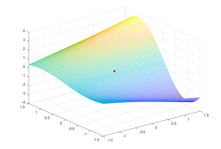
Figure 1: The function used in the proof of Proposition 1, for $\delta=1$. The origin (which fulfills the definition of a $(1,0)$-stationary point) is marked with a red dot. Best viewed in color.

Proof.

Fixing some $\delta>0$, consider the function

$$f(u,v)~{}:=~{}(2\delta+u)\sin\left(\frac{\pi}{2\delta}v\right)$$

(see Fig. 1 for an illustration). This function is differentiable, and its gradient satisfies

$$\nabla f(u,v)~{}=~{}\left(\sin\left(\frac{\pi}{2\delta}v\right)~{},~{}\frac{\pi}{2\delta}(2\delta+u)\cos\left(\frac{\pi}{2\delta}v\right)\right)~{}.$$

First, we note that

$$\frac{1}{2}\left(\nabla f(0,\delta)+\frac{1}{2}\nabla f(0,-\delta)\right)~{}=~{}\frac{1}{2}\left((1,0)+(-1,0)\right)~{}=~{}(0,0),$$

which implies that $(0,0)$ is in the convex hull of the gradients at a distance at most $\delta$ from the origin, hence the origin is a $(\delta,0)$-stationary point. Second, we have that

$$\|\nabla f(u,v)\|^{2}=\sin^{2}\left(\frac{\pi}{2\delta}v\right)+\left(\frac{\pi}{2\delta}\right)^{2}(2\delta+u)^{2}\cos^{2}\left(\frac{\pi}{2\delta}v\right)~{}.$$ (2)

For any $(u,v)$ of norm at most $2\delta$, we must have $|u|\leq 2\delta$, and therefore the above is at most

$$\sin^{2}\left(\frac{\pi}{2\delta}v\right)+\left(\frac{\pi}{2\delta}\right)^{2}(2\delta+2\delta)^{2}\cos^{2}\left(\frac{\pi}{2\delta}v\right)~{}\leq~{}4\pi^{2}\left(\sin^{2}\left(\frac{\pi}{2\delta}v\right)+\cos^{2}\left(\frac{\pi}{2\delta}v\right)\right)~{}=~{}4\pi^{2}~{},$$

which implies that the function is $2\pi$-Lipschitz on a ball of radius $2\delta$ around the origin. Finally, for any $(u,v)$ of norm at most $\delta$, we have $|u|\leq\delta$, so Eq. (2) is at least

$$\sin^{2}\left(\frac{\pi}{2\delta}v\right)+\left(\frac{\pi}{2\delta}\right)^{2}(2\delta-\delta)^{2}\cos^{2}\left(\frac{\pi}{2\delta}v\right)~{}\geq~{}\sin^{2}\left(\frac{\pi}{2\delta}v\right)+\cos^{2}\left(\frac{\pi}{2\delta}v\right)~{}=~{}1~{}.$$

∎

Remark 1.

Although the function $f(\cdot)$ in the proof has a constant Lipschitz parameter only close to the origin, it can be easily modified to be globally Lipschitz and bounded, for example by considering the function

$$\tilde{f}(\mathbf{x})~{}=~{}\begin{cases}f(\mathbf{x})&\|\mathbf{x}\|\leq 2\delta\\ \max\left\{0,2-\frac{\|\mathbf{x}\|}{2\delta}\right\}\cdot f\left(\frac{2\delta}{\|\mathbf{x}\|}\mathbf{x}\right)&\|\mathbf{x}\|>2\delta\end{cases}~{},$$

which is identical to $f(\cdot)$ in a ball of radius $2\delta$ around the origin, but decays to $0$ for larger $\mathbf{x}$, and can be verified to be globally bounded and Lipschitz independent of $\delta$.

This result suggests that we should drop the $\text{conv}\{\cdot\}$ operator from the definition of $(\delta,\epsilon)$-stationarity in Eq. (1), or equivalently, try to find near-approximately-stationary points: Namely, getting $\delta$-close to a point $\mathbf{x}$ such that $\partial f(\mathbf{x})$ contains an element with norm at most $\epsilon$. This is arguably the most natural way to relax the goal of finding $\epsilon$-stationary points, while hopefully still getting meaningful algorithmic guarantees. Unfortunately, we will show in the following section that this already sets the bar too high: For a very large class of gradient-based algorithms (and in fact, all of them under a mild assumption), it is impossible to find near-approximately-stationary point with worst-case finite-time guarantees, for small enough constant $\delta,\epsilon$. Thus, we cannot strengthen the notion of $(\delta,\epsilon)$-stationarity in this manner, and still hope to get similar algorithmic guarantees. In Sec. 3, we further discuss the result and its implications.

2 Hardness of Finding Near-Approximate-Stationary Points

We begin by formalizing the setting in which we prove our hardness result (Subsection 2.1), followed by the main result in Subsection 2.2 and its proof in Subsection 2.3.

2.1 Preliminaries

Generalized Gradients and Stationary points. First, we formalize the notion of gradients and stationary points for nonsmooth functions (which may not be everywhere differentiable). Given a Lipschitz function $f(\cdot)$ and a point $\mathbf{x}$ in its domain, we let $\partial f(\mathbf{x})$ denote the set of generalized gradients (following Clarke (1990) and Zhang et al. (2020)), which is perhaps the most standard extension of the notion of gradients to nonsmooth nonconvex functions. For Lipschitz functions (which are almost everywhere differentiable by Rademacher’s theorem), one simple way to define it is

$$\partial f(\mathbf{x})~{}:=~{}\text{conv}\{\mathbf{u}:\mathbf{u}=\lim_{k\rightarrow\infty}\nabla f(\mathbf{x}_{k}),\mathbf{x}_{k}\rightarrow\mathbf{x}\}$$

(namely, the convex hull of all limit points of $\nabla f(\mathbf{x}_{k})$, over all sequences $\mathbf{x}_{1},\mathbf{x}_{2},\ldots$ of differentiable points of $f(\cdot)$ which converge to $\mathbf{x}$). With this definition, a (Clarke) stationary point with respect to $f(\cdot)$ is a point $\mathbf{x}$ satisfying $\mathbf{0}\in\partial f(\mathbf{x})$. Also, given some $\epsilon\geq 0$, we say that $\mathbf{x}$ is an $\epsilon$-stationary point with respect to $f(\cdot)$, if there is some $\mathbf{u}\in\partial f(\mathbf{x})$ such that $\|\mathbf{u}\|\leq\epsilon$. To make the problem of getting near $\epsilon$-stationary points non-trivial, and following Zhang et al. (2020), we will focus on functions $f(\cdot)$ that are both globally Lipschitz and bounded from below. In particular, we will assume that $f(\mathbf{0})-\inf_{\mathbf{x}}f(\mathbf{x})$ is upper bounded by a constant (this is without loss of generality, as $\mathbf{0}$ can be replaced by any other fixed reference point).

Oracle Complexity. We will study the algorithmic efficiency of the problem using the standard framework of (first-order) oracle complexity (Nemirovsky and Yudin, 1983): Given a class of Lipschitz and bounded functions $\mathcal{F}$ as above, we associate with each $f\in\mathcal{F}$ an oracle, which for any $\mathbf{x}$ in the domain of $f(\cdot)$, returns the value and a (generalized) gradient of $f(\cdot)$ at $\mathbf{x}$. We focus on iterative algorithms which can be described via an interaction with such an oracle: At every iteration $t$, the algorithm chooses an iterate $\mathbf{x}_{t}$, and receives from the oracle a generalized gradient and value of $f(\cdot)$ at $\mathbf{x}_{t}$. The algorithm then uses the values and gradients obtained up to iteration $t$ to choose the point $\mathbf{x}_{t+1}$ in the next iteration. This framework captures essentially all first-order algorithms for black-box optimization. In this framework, we fix some iteration budget $T$, and study the properties of the iterates $\mathbf{x}_{1},\ldots,\mathbf{x}_{T}$ as a function of $T$ and the properties of $\mathcal{F}$.

Algorithmic Families. We will focus on two broad families of algorithms, which together span nearly all algorithms of interest: The first is the class of all deterministic algorithms (denoted as $\mathcal{A}_{det}$), which are all oracle-based algorithms where where $\mathbf{x}_{1}$ is chosen deterministically, and for all $t>1$, $\mathbf{x}_{t}$ is some deterministic function of $\mathbf{x}_{1}$ and the previously observed values and gradients. The second is the class of all linear-span algorithms (denoted as $\mathcal{A}_{span}$), which are all deterministic or randomized oracle-based algorithms that initialize at some $\mathbf{x}_{1}$ (which we will take to be $\mathbf{0}$ without loss of generality), and

$$\forall t>1,~{}~{}\mathbf{x}_{t}~{}\in~{}\text{span}(\mathbf{g}_{1},\ldots,\mathbf{g}_{t-1})~{},$$

with $\mathbf{g}_{i}$ being the gradient provided by the oracle at iteration $i$, given query point $\mathbf{x}_{i}$.

2.2 Main Result

Our main result is the following:

Theorem 1.

There exist a large enough universal constant $C>0$ and a small enough universal constant $c>0$ such that the following holds: For any algorithm in $\mathcal{A}_{det}\cup\mathcal{A}_{span}$, any $T>1$, and any $d\geq 2T$, there is a function $h(\cdot)$ on $\mathbb{R}^{d}$ such that

• $h(\cdot)$ is $C$-Lipschitz, and $h(\mathbf{0})-\inf_{\mathbf{x}}h(\mathbf{x})\leq C$.

• With probability at least $1-T\exp(-cd)$ over the algorithm’s randomness (or deterministically if the algorithm is deterministic), the iterates $\mathbf{x}_{1},\ldots,\mathbf{x}_{T}$ produced by the algorithm satisfy

  $$\inf_{\mathbf{x}\in\mathcal{S}}\min_{t\in\{1,\ldots,T\}}\|\mathbf{x}_{t}-\mathbf{x}\|\geq c~{},$$

  where $\mathcal{S}$ is the set of $c$-stationary points of $f(\cdot)$.

The theorem implies that for a very large family of algorithms, it is impossible to obtain worst-case, finite-time guarantees for finding near-approximately-stationary points of Lipschitz, bounded-from-below functions

Before continuing, we note that the result can be extended to any oracle-based algorithm (randomized or deterministic) under a widely-believed assumption – see remark 5 in the proof for details. We also make two additional remarks:

Remark 2 (More assumptions on $h(\cdot)$).

The Lipschitz functions $h(\cdot)$ used to prove the theorem are based on a simple composition of affine functions, the Euclidean norm function $\mathbf{x}\mapsto\|\mathbf{x}\|$, and the max function. Thus, the result also holds for more specific families of functions considered in the literature, which satisfy additional regularity properties, as long as they contain any Lipschitz function composed as above (for example, Hadamard semi-differentiable functions in Zhang et al. (2020), Whitney-stratifiable functions in Davis et al. (2018), regular functions in Clarke (1990), etc.).

Remark 3 (Strengthening of Proposition 1).

The proof of Thm. 1 uses a construction that actually strengthens Proposition 1: It implies that for any $\delta,\epsilon$ smaller than some constants, there is a Lipschitz, bounded-from-below function on $\mathbb{R}^{d}$, such that the origin is $(\delta,0)$-stationary, yet there are no $\epsilon$-stationary points even at a constant distance from the origin. See remark 6 in the proof for details.

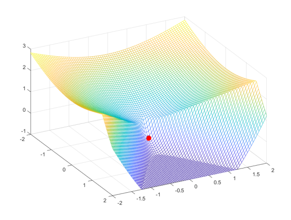
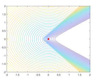
Figure 2: Mesh and Contour plot of the function $\mathbf{x}\mapsto\max\{-1,g_{\mathbf{w}}(\mathbf{x})\}$ on $\mathbb{R}^{2}$, where $\mathbf{w}=(0.3,0)$ and $g_{\mathbf{w}}(\cdot)$ is defined in Lemma 2 (as part of the proof of Thm. 1). The origin is marked with a red dot. Best viewed in color.

The formal proof of the theorem appears in the next subsection, but can be informally described as follows: First, we construct a Lipschitz function on $\mathbb{R}^{d}$, specified by a small vector $\mathbf{w}$, which resembles the norm function $\mathbf{x}\mapsto\|\mathbf{x}\|$ in “most” of $\mathbb{R}^{d}$, but with a “channel” leading away from a neighborhood of the origin in the direction of $\mathbf{w}$, and reaching a completely flat region (see Fig. 2). We emphasize that the graphical illustration is a bit misleading due to the low dimension: In high dimensions, the “channel” and flat region contain a vanishingly small portion of $\mathbb{R}^{d}$. This function has the property of having $\epsilon$-stationary points only in the flat region far away from the origin, in the direction of $\mathbf{w}$, even though the function appears in most places like the norm function $\mathbf{x}\mapsto\|\mathbf{x}\|$ independent of $\mathbf{w}$. As a result, any oracle-based algorithm, that doesn’t happen to hit the vanishingly small region where the function differs from $\mathbf{x}\mapsto\|\mathbf{x}\|$, receives no information about $\mathbf{w}$, and thus cannot determine where the $\epsilon$-stationary points lie. As a result, such an algorithm cannot return near-approximately-stationary points.

Unfortunately, the construction described so far does not work as-is, since the algorithm can always query sufficiently close to the origin (closer than roughly $\|\mathbf{w}\|$), where the gradients do provide information about $\mathbf{w}$. To prevent this, we compose the function with an algorithm-dependent affine mapping, which doesn’t significantly change the function’s properties, but ensures that the algorithm can never get too close to the (mapped) origin. We show that such an affine mapping must exist, based on standard oracle complexity results, which imply that oracle-based algorithms as above cannot get too close to the minimum of a generic convex quadratic function with a bounded number of queries. Using this mapping, and the useful property that $\mathbf{w}$ can be chosen arbitrarily small, leads to our theorem. The full details appear in the following subsection.

Remark 4 (Extension to higher-order algorithms).

Our proof approach is quite flexible, in the sense that for any algorithm, we really only need some function which cannot be optimized to arbitrarily high accuracy, composed with a “channel” construction as above. Since functions of this type also exist for algorithms employing higher-order derivatives beyond gradients (Arjevani et al., 2019), it is unlikely that such higher-order algorithms will circumvent our impossibility result.

2.3 Proof of Thm. 1

We begin by stating the following theorem, which follows from well-known results in oracle complexity (see Nesterov (2018); Nemirovsky and Yudin (1983)):

Theorem 2.

For any $T>1$, any algorithm in $\mathcal{A}_{det}\cup\mathcal{A}_{span}$ and any dimension $d\geq 2T$, there is a vector $\mathbf{x}^{*}\in\mathbb{R}^{d}$ (where $\|\mathbf{x}^{*}\|\leq\frac{1}{2}$) and a positive definite matrix $M\in\mathbb{R}^{d\times d}$ (with minimal and maximal eigenvalues satisfying $\frac{1}{2}\leq\lambda_{\min}(M)\leq\lambda_{\max}(M)\leq 1$), such that the iterates $\mathbf{x}_{1},\ldots,\mathbf{x}_{T}$ produced by the algorithm when ran on the strictly convex quadratic function $f(\mathbf{x}):=(\mathbf{x}-\mathbf{x}^{*})^{\top}M(\mathbf{x}-\mathbf{x}^{*})$ satisfy

$$\min_{t\in\{1,\ldots,T\}}\|\mathbf{x}_{t}-\mathbf{x}^{*}\|~{}\geq~{}\exp(-T)~{}.$$

For completeness, we provide a self-contained proof in Appendix A. Basically, the theorem states that for any algorithm in $\mathcal{A}_{det}\cup\mathcal{A}_{span}$, there is a relatively well-conditioned but still “hard” strictly convex quadratic function, whose minimum cannot be detected with accuracy better than $\exp(-\Omega(T))$.

Remark 5 (Extension to any gradient-based algorithm).

Up to the constants, a lower bound as in Thm. 2 is widely considered to hold (with high-probability) for all oracle-based algorithms, not just for deterministic or linear-span algorithms (see (Nemirovsky and Yudin, 1983; Simchowitz, 2018)). In that case, our Thm. 1 can be easily extended to apply to all oracle-based algorithms which utilize function values and gradients, since the only point in the proof where we really need to restrict the algorithm class is in Thm. 2. Unfortunately, we are not aware of a result in the literature which quite states this, explicitly and in the required form. For example, there are algorithm-independent lower bounds which rely on non-quadratic functions (Woodworth and Srebro, 2017), or apply to quadratics, but not in a regime where $\lambda_{\max}(M)/\lambda_{\min}(M)$ is a constant as in our case (Simchowitz, 2018).

Given the theorem, our first step will be to reduce it to a hardness result for optimizing convex Lipschitz functions of the form $\mathbf{x}\mapsto\|M^{1/2}(\mathbf{x}-\mathbf{x}^{*})\|$:

Lemma 1.

For any algorithm in $\mathcal{A}_{det}\cup\mathcal{A}_{span}$, any $T>1$ and any dimension $d\geq 2T$, there is a vector $\mathbf{x}^{*}\in\mathbb{R}^{d}$ (where $\|\mathbf{x}^{*}\|\leq\frac{1}{2}$) and a positive definite matrix $M\in\mathbb{R}^{d\times d}$ (with $\frac{1}{2}\leq\lambda_{\min}(M)\leq\lambda_{\max}(M)\leq 1$), such that the convex function

$$\tilde{f}(\mathbf{x})~{}:=~{}\|M^{1/2}(\mathbf{x}-\mathbf{x}^{*})\|$$

satisfies the following:

• $\tilde{f}(\cdot)$ is $\frac{1}{\sqrt{2}}$-Lipschitz, and $\tilde{f}(\mathbf{0})\leq\frac{1}{2}$.

• If we run the algorithm on $\tilde{f}(\cdot)$, then $\min_{t\in\{1,\ldots,T\}}\|\mathbf{x}_{t}-\mathbf{x}^{*}\|\geq\exp(-T)$.

Proof.

We will start with the second bullet. Fix some algorithm $A$ in $\mathcal{A}_{det}\cup\mathcal{A}_{span}$, and assume by contradiction that for any $\mathbf{x}^{*},M$ satisfying the conditions in the lemma, the algorithm runs on $\tilde{f}(\cdot)$ and produces iterates such that $\min_{t\in\{1,\ldots,T\}}\|\mathbf{x}_{t}-\mathbf{x}^{*}\|<\exp(-T)$ (either deterministically if the algorithm is deterministic, or for some realization of its random coin flips, if it is randomized). But then, we argue that given access to gradients and values of $f(\mathbf{x}):=\tilde{f}^{2}(\mathbf{x})=(\mathbf{x}-\mathbf{x}^{*})^{\top}M(\mathbf{x}-\mathbf{x}^{*})$, we can use $A$ to specify another algorithm in $\mathcal{A}_{det}\cup\mathcal{A}_{span}$ that runs on $f(\cdot)$ and produces points $\mathbf{x}_{1},\ldots,\mathbf{x}_{T}$ such that $\min_{t\in\{1,\ldots,T\}}\|\mathbf{x}_{t}-\mathbf{x}^{*}\|<\exp(-T)$, contradicting Thm. 2. To see why, note that given access to an oracle returning values and gradients of $f(\cdot)$ at $\mathbf{x}$, we can simulate an oracle returning gradients and values of $\tilde{f}(\cdot)$ at $\mathbf{x}$ via the easily-verified formulaes

$$\tilde{f}(\mathbf{x})=\sqrt{f(\mathbf{x})}~{}~{}~{}\text{and}~{}~{}~{}\nabla\tilde{f}(\mathbf{x})=\frac{1}{2\sqrt{f(\mathbf{x})}}\nabla f(\mathbf{x})$$

(and for $\mathbf{x}=\mathbf{x}^{*}$ where $\tilde{f}(\cdot)$ is not differentiable, we can just return the value $0$ and the generalized gradient $\mathbf{0}$). We then feed the responses of this simulated oracle to $A$, and get the resulting $\mathbf{x}_{1},\ldots,\mathbf{x}_{T}$. This give us a new algorithm $A^{\prime}$, which is easily verified to be in $\mathcal{A}_{det}\cup\mathcal{A}_{span}$ if the original algorithm $A$ is in $\mathcal{A}_{det}\cup\mathcal{A}_{span}$.

It remains to prove the second bullet in the lemma. First, we have $\tilde{f}(\mathbf{0})=\|M^{1/2}\mathbf{x}^{*}\|\leq\sqrt{\|M\|}\|\mathbf{x}^{*}\|\leq\frac{1}{2}$. Second, we note that for any $\mathbf{x}\neq\mathbf{x}^{*}$, $\tilde{f}(\cdot)$ is differentiable and satisfies

$$\|\nabla\tilde{f}(\mathbf{x})\|~{}=~{}\frac{\|M(\mathbf{x}-\mathbf{x}^{*})\|}{2\|M^{1/2}(\mathbf{x}-\mathbf{x}^{*})\|}~{}\leq~{}\frac{\lambda_{\max}(M)\cdot\|\mathbf{x}-\mathbf{x}^{*}\|}{2\sqrt{\lambda_{\min}(M)}\cdot\|\mathbf{x}-\mathbf{x}^{*}\|}~{}=~{}\frac{\lambda_{\max}(M)}{2\sqrt{\lambda_{\min}(M)}}~{},$$

which by the conditions on $M$, is at most $\frac{1}{2\sqrt{1/2}}=\frac{1}{\sqrt{2}}$. ∎

Next, we define a function $g(\cdot)$ with two properties: It is identical to $\mathbf{x}\mapsto\|\mathbf{x}\|$ in parts of $\mathbb{R}^{d}$ (in fact, as we will see later, in “almost” all of $\mathbb{R}^{d}$), yet unlike the function $\mathbf{x}\mapsto\|\mathbf{x}\|$, it has no stationary points, or even $\epsilon$-stationary points.

Lemma 2.

Fix some vector $\mathbf{w}\neq\mathbf{0}$ in $\mathbb{R}^{d}$, and define the function

$$g_{\mathbf{w}}(\mathbf{x})~{}:=~{}\|\mathbf{x}\|-\left[4\bar{\mathbf{w}}^{\top}(\mathbf{x}+\mathbf{w})-2\|\mathbf{x}+\mathbf{w}\|\right]_{+},$$

where $\bar{\mathbf{u}}:=\mathbf{u}/\|\mathbf{u}\|$ for any vector $\mathbf{u}$, and $[v]_{+}:=\max\{v,0\}$. Then $g_{\mathbf{w}}(\cdot)$ is $7$-Lipschitz, and has no $\epsilon$-stationary points for any $\epsilon<\frac{1}{\sqrt{2}}$ .

Proof.

In the proof, we will drop the $\mathbf{w}$ subscript and refer to $g_{\mathbf{w}}(\cdot)$ as $g(\cdot)$.

The functions $\mathbf{x}\mapsto\|\mathbf{x}\|$, $\mathbf{x}\mapsto 4\bar{\mathbf{w}}^{\top}(\mathbf{x}+\mathbf{w})$, $\mathbf{x}\mapsto 2\|\mathbf{x}+\mathbf{w}\|$ and $x\mapsto\max\{0,x\}$ are respectively $1$-Lipschitz, $4$-Lipschitz, $2$-Lipschitz and $1$-Lipschitz, from which it immediately follows that $g(\cdot)$ is $1+4+2=7$ Lipschitz. Thus, it only remains to show that $g(\cdot)$ has no $\epsilon$-stationary points.

It is easily seen that the function $g(\cdot)$ is not differentiable at only $3$ possible regions: (1) $\mathbf{x}=\mathbf{0}$, (2) $\mathbf{x}=-\mathbf{w}$, and (3) $\{\mathbf{x}:4\bar{\mathbf{w}}^{\top}(\mathbf{x}+\mathbf{w})-2\|\mathbf{x}+\mathbf{w}\|=0\}$ (or equivalently, $\{\mathbf{x}:\bar{\mathbf{w}}^{\top}(\overline{\mathbf{x}+\mathbf{w}})=\frac{1}{2}\}$ if we exclude $\mathbf{x}=-\mathbf{w}$), which are all measure-zero sets in $\mathbb{R}^{d}$. At any other point, $g(\cdot)$ is differentiable and the gradient satisfies

$$\nabla g(\mathbf{x})=\bar{\mathbf{x}}-\mathbf{1}_{\bar{\mathbf{w}}^{\top}(\overline{\mathbf{x}+\mathbf{w}})>\frac{1}{2}}\cdot\left(4\bar{\mathbf{w}}-2(\overline{\mathbf{x}+\mathbf{w}})\right)~{}.$$

Moreover, at those differentiable points, if $\bar{\mathbf{w}}^{\top}(\overline{\mathbf{x}+\mathbf{w}})<\frac{1}{2}$ then

$$\|\nabla g(\mathbf{x})\|~{}=~{}\|\bar{\mathbf{x}}\|~{}=~{}1~{},$$

and if $\bar{\mathbf{w}}^{\top}(\overline{\mathbf{x}+\mathbf{w}})>\frac{1}{2}$, then by the triangle inequality,

$$\|\nabla g(\mathbf{x})\|~{} =~{}\|\bar{\mathbf{x}}-\left(4\bar{\mathbf{w}}-2(\overline{\mathbf{x}+\mathbf{w}})\right)\|~{}=~{}\|4\bar{\mathbf{w}}-2(\overline{\mathbf{x}+\mathbf{w}})-\bar{\mathbf{x}}\|$$

$$\geq~{}4\|\bar{\mathbf{w}}\|-2\|\overline{\mathbf{x}+\mathbf{w}}\|-\|\bar{\mathbf{x}}\|~{}=~{}4-2-1=1~{}.$$

Thus, no differentiable point of $g$ is even $0.99$-stationary. It remains to show that even the non-differentiable points of $g$ are not $\epsilon$-stationary for any $\epsilon<\frac{1}{\sqrt{2}}$. To do so, we will use the facts that $\partial(g_{1}+g_{2})\subseteq\partial g_{1}+\partial g_{2}$, and that if $g_{1}$ is univariate, $\partial(g_{1}\circ g_{2})(\mathbf{x})\subseteq\text{conv}\{r_{1}\mathbf{r}_{2}:r_{1}\in\partial g_{1}(g_{2}(\mathbf{x})),\mathbf{r}_{2}\in\partial g_{2}(\mathbf{x})\}$ (see Clarke (1990)).

• At $\mathbf{x}=\mathbf{0}$, we have

  $$\partial g(\mathbf{x})~{}\subseteq~{}\text{conv}\{\mathbf{u}-2\bar{\mathbf{w}}~{}:~{}\|\mathbf{u}\|\leq 1\}~{}=~{}\{\mathbf{u}-2\bar{\mathbf{w}}~{}:~{}\|\mathbf{u}\|\leq 1\}~{}.$$

  Any element in this set has a norm of $\|\mathbf{u}-2\bar{\mathbf{w}}\|=\|2\bar{\mathbf{w}}-\mathbf{u}\|\geq 2\|\bar{\mathbf{w}}\|-\|\mathbf{u}\|\geq 2-1=1$ by the triangle inequality. Thus, $\mathbf{x}=0$ is not $\epsilon$-stationary for any $\epsilon<1$.

• At $\mathbf{x}=-\mathbf{w}$, we have

  $$\partial g(\mathbf{x})~{} \subseteq~{}\text{conv}\{-\bar{\mathbf{w}}-v\cdot(4\bar{\mathbf{w}}-2\mathbf{u}):v\in[0,1],\|\mathbf{u}\|\leq 1\}$$

  $$=~{}\text{conv}\{2v\mathbf{u}-(1+4v)\bar{\mathbf{w}}:v\in[0,1],\|\mathbf{u}\|\leq 1\}~{}.$$

  For any element in the set $\{2v\mathbf{u}-(1+4v)\bar{\mathbf{w}}:v\in[0,1],\|\mathbf{u}\|\leq 1\}$ (corresponding to some $v,\mathbf{u}$), its inner product with $-\bar{\mathbf{w}}$ is

  $$-2v\bar{\mathbf{w}}^{\top}\mathbf{u}+(1+4v)\geq-2v+(1+4v)\geq 1~{}.$$

  Thus, any element in the convex hull of this set, which contains $\partial g(\mathbf{x})$, has an inner product of at least $1$ with $-\bar{\mathbf{w}}$. Since $-\bar{\mathbf{w}}$ is a unit vector, it follows that the norm of any element in $\partial g(\mathbf{x})$ is at least $1$, so this point is not $\epsilon$-stationary for any $\epsilon<1$.

• At any $\mathbf{x}$ in the set $\{\mathbf{x}:\bar{\mathbf{w}}^{\top}(\overline{\mathbf{x}+\mathbf{w}})=\frac{1}{2}\}\setminus\{\mathbf{0},-\mathbf{w}\}$, we have

  $$\partial g(\mathbf{x})~{} \subseteq~{}\text{conv}\left\{\bar{\mathbf{x}}-v\cdot\left(4\bar{\mathbf{w}}-2(\overline{\mathbf{x}+\mathbf{w}})\right)~{}:~{}v\in[0,1]\right\}$$

  $$=~{}\left\{\bar{\mathbf{x}}-v\cdot\left(4\bar{\mathbf{w}}-2(\overline{\mathbf{x}+\mathbf{w}})\right)~{}:~{}v\in[0,1]\right\}$$ (3)

  $$=~{}\left\{\left(\frac{1}{\|\mathbf{x}\|}+\frac{2v}{\|\mathbf{x}+\mathbf{w}\|}\right)\mathbf{x}-\left(\frac{4v}{\|\mathbf{w}\|}-\frac{2v}{\|\mathbf{x}+\mathbf{w}\|}\right)\mathbf{w}~{}:~{}v\in[0,1]\right\}~{}.$$ (4)

  Let $\mathbf{x}=\mathbf{x}_{|}+\mathbf{x}_{\perp}$, where $\mathbf{x}_{\perp}=(I-\bar{\mathbf{w}}\bar{\mathbf{w}}^{\top})\mathbf{x}$ is the component of $\mathbf{x}$ orthogonal to $\mathbf{w}$, and $\mathbf{x}_{|}\in\text{span}(\mathbf{w})$. Thus, any element in $\partial g(\mathbf{x})$ can be written as

  $$\left(\frac{1}{\|\mathbf{x}\|}+\frac{2v}{\|\mathbf{x}+\mathbf{w}\|}\right)\mathbf{x}_{\perp}+a\cdot\mathbf{w}$$

  for some scalar $a$. Since $\mathbf{w}$ is orthogonal to $\mathbf{x}_{\perp}$, the norm of this element is at least

  $$\left(\frac{1}{\|\mathbf{x}\|}+\frac{2v}{\|\mathbf{x}+\mathbf{w}\|}\right)\|\mathbf{x}_{\perp}\|~{}\geq~{}\frac{1}{\|\mathbf{x}\|}\cdot\|\mathbf{x}_{\perp}\|~{}.$$

  Noting that

  $$\|\mathbf{x}_{\perp}\|^{2}=\mathbf{x}^{\top}(I-\bar{\mathbf{w}}\bar{\mathbf{w}}^{\top})^{2}\mathbf{x}=\mathbf{x}^{\top}(I-\bar{\mathbf{w}}\bar{\mathbf{w}}^{\top})\mathbf{x}=\|\mathbf{x}\|^{2}-(\bar{\mathbf{w}}^{\top}\mathbf{x})^{2}=\|\mathbf{x}\|^{2}(1-(\bar{\mathbf{w}}^{\top}\bar{\mathbf{x}})^{2})$$

  and plugging into the above, it follows that the norm is at least $\sqrt{(1-(\bar{\mathbf{w}}^{\top}\bar{\mathbf{x}})^{2})}$.

  Now, let us suppose that there exists an element in $\partial g(\mathbf{x})$ with norm at most $\epsilon$. By the above, it follows that

  $$\sqrt{(1-(\bar{\mathbf{w}}^{\top}\bar{\mathbf{x}})^{2})}\leq\epsilon~{}.$$ (5)

  However, we will show that for any $\epsilon<\frac{1}{\sqrt{2}}$, we must arrive at a contradiction, which implies that $\mathbf{x}$ cannot be $\epsilon$-stationary for $\epsilon<\frac{1}{\sqrt{2}}$. To that end, let us consider two cases:

  • If $\bar{\mathbf{w}}^{\top}\bar{\mathbf{x}}\leq 0$, then by Eq. (5), we must have $\bar{\mathbf{w}}^{\top}\bar{\mathbf{x}}\leq-\sqrt{1-\epsilon^{2}}$. But then, for any $\mathbf{u}\in\partial g(\mathbf{x})$, by Eq. (3) and our assumption that $\bar{\mathbf{w}}^{\top}(\overline{\mathbf{x}+\mathbf{w}})=\frac{1}{2}$,

    $$\bar{\mathbf{w}}^{\top}\mathbf{u}~{}=~{}\bar{\mathbf{w}}^{\top}\bar{\mathbf{x}}-v\cdot\left(4-2\cdot\frac{1}{2}\right)~{}\leq~{}-\sqrt{1-\epsilon^{2}}-3v~{}\leq~{}-\sqrt{1-\epsilon^{2}}.$$

    This implies that $\|\mathbf{u}\|\geq\sqrt{1-\epsilon^{2}}$ for any $\mathbf{u}\in\partial g(\mathbf{x})$. Thus, if there was some $\mathbf{u}\in\partial g(\mathbf{x})$ with norm at most $\epsilon$, we get that $\epsilon\geq\sqrt{1-\epsilon^{2}}$, which cannot hold if $\epsilon<\frac{1}{\sqrt{2}}$.

  • If $\bar{\mathbf{w}}^{\top}\bar{\mathbf{x}}>0$, then by Eq. (5), we have $\bar{\mathbf{w}}^{\top}\bar{\mathbf{x}}\geq\sqrt{1-\epsilon^{2}}$. Hence,

    $$\bar{\mathbf{w}}^{\top}(\mathbf{x}+\mathbf{w})~{}\geq~{}\|\mathbf{x}\|\sqrt{1-\epsilon^{2}}+\|\mathbf{w}\|~{}\geq~{}(\|\mathbf{x}\|+\|\mathbf{w}\|)\sqrt{1-\epsilon^{2}}~{}\geq~{}\|\mathbf{x}+\mathbf{w}\|\sqrt{1-\epsilon^{2}}~{}.$$

    However, dividing both sides by $\|\mathbf{x}+\mathbf{w}\|$, we get that $\bar{\mathbf{w}}^{\top}(\overline{\mathbf{x}+\mathbf{w}})~{}\geq~{}\sqrt{1-\epsilon^{2}}$. If $\epsilon<\frac{1}{\sqrt{2}}$, it follows that $\bar{\mathbf{w}}^{\top}(\overline{\mathbf{x}+\mathbf{w}})>\frac{1}{\sqrt{2}}$, which contradicts our assumption that $\mathbf{x}$ satisfies $\bar{\mathbf{w}}^{\top}(\overline{\mathbf{x}+\mathbf{w}})=\frac{1}{2}$.

∎

Remark 6.

The function

$$\tilde{g}_{\mathbf{w}}(\mathbf{x}):=\max\{g_{\mathbf{w}}(\mathbf{0})-1~{},~{}g_{\mathbf{w}}(\mathbf{x})\}~{},$$

where $g_{\mathbf{w}}(\cdot)$ is as defined in Lemma 2, actually strengthens Proposition 1 from the introduction: According to the lemma, $g_{\mathbf{w}}(\cdot)$ is $7$-Lipschitz and has no $\epsilon$-stationary points for $\epsilon<1/\sqrt{2}$. Therefore, it is easily verified that for any $\mathbf{w}$, $\tilde{g}_{\mathbf{w}}(\cdot)$ is $7$-Lipschitz, bounded from below, and any $\epsilon$-stationary point is at a distance of at least $1/7$ from the origin. However, we also claim that the origin is a $(\delta,0)$-stationary point for any $\delta\in\left(0,1/7\right)$. To see this, note first that for such $\delta$, by the Lipschitz property of $g_{\mathbf{w}}(\cdot)$, we have $\tilde{g}_{\mathbf{w}}(\mathbf{x})=g_{\mathbf{w}}(\mathbf{x})$ in a $\delta$-neighborhood of the origin. Fix any $\mathbf{w}$ such that $\|\mathbf{w}\|=\frac{\delta}{2}$, and let $\mathbf{v}$ be any vector of norm $\delta$ orthogonal to $\mathbf{w}$. It is easily verified that $\bar{\mathbf{w}}^{\top}(\overline{\mathbf{v}+\mathbf{w}})<\frac{1}{2}$, in which case

$$\nabla\tilde{g}_{\mathbf{w}}(\mathbf{v})~{}=~{}\nabla g_{\mathbf{w}}(\mathbf{v})~{}=~{}\bar{\mathbf{v}}~{},$$

and therefore $\frac{1}{2}\left(\nabla\tilde{g}_{\mathbf{w}}(\mathbf{v})+\nabla\tilde{g}_{\mathbf{w}}(-\mathbf{v})\right)=\mathbf{0}$.

Lemma 3.

Fix any algorithm in $\mathcal{A}_{det}\cup\mathcal{A}_{span}$, any $T>1$ and any $d\geq 2T$. Define the function

$$h_{\mathbf{w}}(\mathbf{x})~{} :=~{}\max\{-1~{},~{}g_{\mathbf{w}}(M^{1/2}(\mathbf{x}-\mathbf{x}^{*}))\}$$

$$=~{}\max\left\{-1,\|M^{1/2}(\mathbf{x}-\mathbf{x}^{*})\|-\left[4\bar{\mathbf{w}}^{\top}(M^{1/2}(\mathbf{x}-\mathbf{x}^{*})+\mathbf{w})-2\|M^{1/2}(\mathbf{x}-\mathbf{x}^{*})+\mathbf{w}\|\right]_{+}\right\}~{},$$

where $M,\mathbf{w}^{*}$ are as defined in Lemma 1, $g_{\mathbf{w}}(\cdot)$ is as defined in Lemma 2, and $\mathbf{w}$ is a vector of norm $\frac{1}{300}\exp(-T)$ in $\mathbb{R}^{d}$. Then:

• $h_{\mathbf{w}}(\cdot)$ is $7$-Lipschitz, and satisfies $h_{\mathbf{w}}(\mathbf{0})-\inf_{\mathbf{x}}h_{\mathbf{w}}(\mathbf{x})\leq\frac{3}{2}$.

• Any $\epsilon$-stationary point $\mathbf{x}$ of $h_{\mathbf{w}}(\cdot)$ for $\epsilon<\frac{1}{2\sqrt{2}}$ satisfies $h_{\mathbf{w}}(\mathbf{x})=-1$.

• There exists a choice of $\mathbf{w}$, such that if we run the algorithm on $h_{\mathbf{w}}(\cdot)$, then with probability at least $1-T\exp(-d/18)$ over the algorithm’s randomness (or deterministically if the algorithm is deterministic), the algorithm’s iterates $\mathbf{x}_{1},\ldots,\mathbf{x}_{T}$ satisfy $\min_{t\in\{1,\ldots,T\}}h_{\mathbf{w}}(\mathbf{x}_{t})>0$.

Proof.

The Lipschitz bound follows from the facts that $z\mapsto\max\{-1,z\}$ is $1$-Lipschitz, $\mathbf{x}\mapsto M^{1/2}(\mathbf{x}-\mathbf{x}^{*})$ is $\|M^{1/2}\|\leq 1$-Lipschitz, and that $g_{\mathbf{w}}$ is $7$-Lipschitz by Lemma 2. Moreover, we clearly have $\inf_{\mathbf{x}}h_{\mathbf{w}}(\mathbf{x})\geq-1$, and by definition of $h_{\mathbf{w}}(\cdot)$ and Lemma 1,

$$h_{\mathbf{w}}(\mathbf{0})~{}\leq~{}\|-M^{1/2}\mathbf{x}^{*}\|=\tilde{f}(\mathbf{0})\leq\frac{1}{2}~{}.$$

Combining the two observations establishes the first bullet in the lemma.

As to the second bullet, let $\tilde{g}(\mathbf{x}):=g_{\mathbf{w}}(M^{1/2}(\mathbf{x}-\mathbf{x}^{*}))$ (so that $h_{\mathbf{w}}(\mathbf{x})=\max\{-1,\tilde{g}(\mathbf{x})\}$). It is easily verified that $\mathbf{u}\in\partial g_{\mathbf{w}}(\mathbf{x})$ if and only if $M^{1/2}\mathbf{u}\in\partial\tilde{g}(\mathbf{x}+\mathbf{x}^{*})$. By Lemma 2, $g_{\mathbf{w}}$ has no $\epsilon$-stationary point for $\epsilon<\frac{1}{\sqrt{2}}$, which implies that $\tilde{g}(\mathbf{x})$ has no $\epsilon$-stationary points for any $\epsilon$ less than $\lambda_{\min}(M^{1/2})\frac{1}{\sqrt{2}}\geq\frac{1}{2\sqrt{2}}$. But since $h_{\mathbf{w}}(\mathbf{x})=\max\{-1,\tilde{g}(\mathbf{x})\}$, it follows that any $\epsilon$-stationary points of $h_{\mathbf{w}}(\cdot)$ must be arbitrarily close to the region where $h_{\mathbf{w}}(\cdot)$ is different than $\tilde{g}(\cdot)$, namely where it takes a value of $-1$. Since $h_{\mathbf{w}}(\cdot)$ is Lipschitz, it follows that its value is $-1$ at the $\epsilon$-stationary point as well.

We now turn to establish the third bullet in the lemma. A crucial observation here is that

$$h_{\mathbf{w}}(\mathbf{x})~{}=~{}g_{\mathbf{w}}(M^{1/2}(\mathbf{x}-\mathbf{x}^{*}))~{}=~{}\tilde{f}(\mathbf{x})~{}~{}~{}~{}\forall\mathbf{x}:\bar{\mathbf{w}}^{\top}\left(\overline{M^{1/2}(\mathbf{x}-\mathbf{x}^{*})+\mathbf{w}}\right)\leq\frac{1}{2}~{},$$ (6)

where $\tilde{f}(\mathbf{x})=\|M^{1/2}(\mathbf{x}-\mathbf{x}^{*})\|$ is the “hard function” defined in Lemma 1. To see why, note first that by definition of $g_{\mathbf{w}}(\cdot)$ in Lemma 2, for any $\mathbf{x}$ which satisfies the condition in the displayed equation above, we have $g_{\mathbf{w}}(M^{1/2}(\mathbf{x}-\mathbf{x}^{*}))=\|M^{1/2}(\mathbf{x}-\mathbf{x}^{*})\|=\tilde{f}(\mathbf{x})$. On the other hand, since this is a non-negative function, it follows that it also equals $\max\{-1,g_{\mathbf{w}}(M^{1/2}(\mathbf{x}-\mathbf{x}^{*}))\}=h_{\mathbf{w}}(\mathbf{x})$ for such $\mathbf{x}$, establishing the displayed equation above.

Next, we will show that Eq. (6) also holds over a set of $\mathbf{x}$’s which have a more convenient form. To do so, fix some $\mathbf{x}$ which satisfies the opposite condition $\bar{\mathbf{w}}^{\top}\left(\overline{M^{1/2}(\mathbf{x}-\mathbf{x}^{*})+\mathbf{w}}\right)>\frac{1}{2}$. Then multiplying both sides by $\|M^{1/2}(\mathbf{x}-\mathbf{x}^{*})+\mathbf{w}\|$, we get

$$\bar{\mathbf{w}}^{\top}M^{1/2}(\mathbf{x}-\mathbf{x}^{*})+\bar{\mathbf{w}}^{\top}\mathbf{w}~{}>~{}\frac{1}{2}\|M^{1/2}(\mathbf{x}-\mathbf{x}^{*})+\mathbf{w}\|~{}\geq~{}\frac{1}{2}\left(\|M^{1/2}(\mathbf{x}-\mathbf{x}^{*})\|-\|\mathbf{w}\|\right)~{}.$$

Since $\frac{1}{2}\leq\lambda_{\min}(M)\leq\lambda_{\max}(M)\leq 1$ by Lemma 1, it follows that

$$\bar{\mathbf{w}}^{\top}M^{1/2}(\mathbf{x}-\mathbf{x}^{*})+\|\mathbf{w}\|~{}>~{}\frac{1}{2}\left(\frac{1}{\sqrt{2}}\|\mathbf{x}-\mathbf{x}^{*}\|-\|\mathbf{w}\|\right)~{}.$$

For $\mathbf{x}=\mathbf{x}^{*}$, the condition above is trivially satisfied. For $\mathbf{x}\neq\mathbf{x}^{*}$, dividing both sides by $\|M^{1/2}(\mathbf{x}-\mathbf{x}^{*})\|$ (which is between $\|\mathbf{x}-\mathbf{x}^{*}\|$ and $\frac{1}{2}\|\mathbf{x}-\mathbf{x}^{*}\|$) and simplifying a bit, we get that

$$\bar{\mathbf{w}}^{\top}\left(\overline{M^{1/2}(\mathbf{x}-\mathbf{x}^{*})}\right)~{}>~{}\frac{1}{2\sqrt{2}}-\frac{3\|\mathbf{w}\|}{2\cdot\frac{1}{2}\|\mathbf{x}-\mathbf{x}^{*}\|}~{}=~{}\frac{1}{2\sqrt{2}}-\frac{\exp(-T)}{100\|\mathbf{x}-\mathbf{x}^{*})\|}~{}.$$

Noting that any $\mathbf{x}$ which does not satisfy the condition in Eq. (6) satisfy the condition above, we get that Eq. (6) implies

$$h_{\mathbf{w}}(\mathbf{x})=\tilde{f}(\mathbf{x})=\|M^{1/2}(\mathbf{x}-\mathbf{x}^{*})\|~{}~{}~{}\forall\mathbf{x}\neq\mathbf{x}^{*}~{}\text{s.t.}~{}\bar{\mathbf{w}}^{\top}\left(\overline{M^{1/2}(\mathbf{x}-\mathbf{x}^{*})}\right)~{}\leq~{}\frac{1}{2\sqrt{2}}-\frac{\exp(-T)}{100\|\mathbf{x}-\mathbf{x}^{*}\|}~{}.$$ (7)

With this equation in hand, let us first establish the third bullet of the lemma, assuming the algorithm we consider is deterministic. In order to do so, let $\mathbf{x}_{1}^{\tilde{f}},\ldots,\mathbf{x}_{T}^{\tilde{f}}$ be the (fixed) iterates produced by the algorithm when ran on $\tilde{f}(\cdot)$, and choose $\mathbf{w}$ in $h_{\mathbf{w}}(\cdot)$ to be any vector orthogonal to $\{M^{1/2}(\mathbf{x}_{t}^{\tilde{f}}-\mathbf{x}^{*})\}_{t=1}^{T}$ (which is possible since the dimension $d$ is larger than $T$). By Lemma 1, we know that for all $t$, $\|\mathbf{x}_{t}^{\tilde{f}}-\mathbf{x}^{*}\|\geq\exp(-T)$, in which case we have

$$\bar{\mathbf{w}}^{\top}\left(\overline{M^{1/2}(\mathbf{x}_{t}^{\tilde{f}}-\mathbf{x}^{*})}\right)~{}=~{}0~{}<~{}\frac{1}{2\sqrt{2}}-\frac{\exp(-T)}{100\exp(-T)}~{}\leq~{}\frac{1}{2\sqrt{2}}-\frac{\exp(-T)}{100\|\mathbf{x}_{t}^{\tilde{f}}-\mathbf{x}^{*}\|}~{}.$$

Thus, $\mathbf{x}_{t}^{\tilde{f}}$ satisfies the condition in Eq. (7), and as a result, $h_{\mathbf{w}}(\mathbf{x}_{t}^{\tilde{f}})=\tilde{f}(\mathbf{x}_{t}^{\tilde{f}})$ for all $t$. Moreover, using the fact that $\mathbf{x}_{t}^{\tilde{f}}$ is bounded away from $\mathbf{x}^{*}$, it is easily verified that the condition in Eq. (7) also holds for $\mathbf{x}$ in a small local neighborhood of $\mathbf{x}_{t}^{\tilde{f}}$, so actually $h_{\mathbf{w}}(\cdot)$ is identical to $\tilde{f}(\cdot)$ on these local neigborhoods, implying the same values and gradients at $\mathbf{x}_{t}^{\tilde{f}}$. As a result, if we run the algorithm on $h_{\mathbf{w}}(\cdot)$ rather than $f(\cdot)$, then the iterates $\mathbf{x}_{1},\ldots,\mathbf{x}_{T}$ produced are identical to $\mathbf{x}_{1}^{\tilde{f}},\ldots,\mathbf{x}_{T}^{\tilde{f}}$. Since $\|\mathbf{x}_{t}^{\tilde{f}}-\mathbf{x}^{*}\|>0$, we have $h_{\mathbf{w}}(\mathbf{x}_{t})=\tilde{f}(\mathbf{x}_{t}^{\tilde{f}})=\|M^{1/2}(\mathbf{x}_{t}^{\tilde{f}}-\mathbf{x}^{*})\|>0$ for all $t$ as required.

We now turn to establish the third bullet of the lemma, assuming the algorithm is randomized. As before, we let $\mathbf{x}_{1}^{\tilde{f}},\ldots,\mathbf{x}_{T}^{\tilde{f}}$ denote the iterates produced by the algorithm when ran on $\tilde{f}(\cdot)$ (only that now they are possibly random, based on the algorithm’s random coin flips). The proof idea is roughly the same, but here the iterates may be randomized, so we cannot choose $\mathbf{w}$ in some fixed manner. Instead, we will pick $\mathbf{w}$ independently and uniformly at random among vectors of norm $\frac{1}{300}\exp(-T)$, and show that for any realization of the algorithm’s random coin flips, with probability at least $1-T\exp(-d/18)$ over $\mathbf{w}$, $\min_{t}h_{\mathbf{w}}(\mathbf{x}_{t})>0$. This implies that there exists some fixed choice of $\mathbf{w}$, for which $\min_{t}h_{\mathbf{w}}(\mathbf{x}_{t})>0$ with the same high probability over the algorithm’s randomness, as required. To proceed, we collect two observations:

1. By Lemma 1, we know that for any realization of the algorithm’s random coin flips, $\min_{t\in\{1,\ldots,T\}}\|\mathbf{x}_{t}-\mathbf{x}^{*}\|\geq\exp(-T)>0$.

2. If we fix some unit vectors $\mathbf{u}_{1},\ldots,\mathbf{u}_{T}$ in $\mathbb{R}^{d}$, and pick a unit vector $\mathbf{u}$ uniformly at random, then by a union bound and a standard large deviation bound (e.g., Tkocz (2012)), $\Pr(\max_{t}\mathbf{u}^{\top}\mathbf{u}_{t}\geq a)\leq T\cdot\Pr(\mathbf{u}^{\top}\mathbf{u}_{1}\geq a)\leq T\exp(-da^{2}/2)$. Taking $\mathbf{w}=\mathbf{u}$, $\mathbf{u}_{t}=\overline{M^{1/2}(\mathbf{x}_{t}^{\tilde{f}}-\mathbf{x}^{*})}$ for all $t$ (for some realization of $\mathbf{x}_{t}^{\tilde{f}}$), and $a=1/3$, it follows that for any realization of the algorithm’s random coin flips, $\max_{t}\mathbf{w}^{\top}(\overline{M^{1/2}\mathbf{x}_{t}^{\tilde{f}}-\mathbf{x}^{*}})\geq 1/3$ with probability at most $T\exp(-d/18)$ over the choice of $\mathbf{w}$.

Combining the two observations, we get that for any realization of the algorithm’s coin flips, with probability at least $1-T\exp(-d/18)$ over the choice of $\mathbf{w}$, it holds for all $\mathbf{x}_{1}^{\tilde{f}},\ldots,\mathbf{x}_{T}^{\tilde{f}}$ that

$$\bar{\mathbf{w}}^{\top}\left(\overline{M^{1/2}(\mathbf{x}_{t}^{\tilde{f}}-\mathbf{x}^{*})}\right)~{}<\frac{1}{3}~{}<~{}\frac{1}{2\sqrt{2}}-\frac{\exp(-T)}{100\exp(-T)}~{}\leq~{}\frac{1}{2\sqrt{2}}-\frac{\exp(-T)}{100\|\mathbf{x}-\mathbf{x}^{*}\|}~{},$$

as well as $\|\mathbf{x}_{t}^{\tilde{f}}-\mathbf{x}^{*}\|>0$. Using the same argument as in the deterministic case, it follows from Eq. (7) that $h_{\mathbf{w}}(\cdot)$ and $\tilde{f}(\cdot)$ coincide in small neighborhoods around $\mathbf{x}_{1}^{\tilde{f}},\ldots,\mathbf{x}_{T}^{\tilde{f}}$, with probability at least $1-T\exp(-d/18)$. Since the algorithm’s iterates depend only on the local values/gradients returned by the oracle, it follows that for any realization of the algorithm’s coin flips, with probability at least $1-T\exp(-d/18)$ over the choice of $\mathbf{w}$, the iterates $\mathbf{x}_{1},\ldots,\mathbf{x}_{T}$ and $\mathbf{x}_{1}^{\tilde{f}},\ldots,\mathbf{x}_{T}^{\tilde{f}}$ are going to be identical, and satisfy

$$\min_{t}h_{\mathbf{w}}(\mathbf{x}_{t})=\min_{t}h_{\mathbf{w}}(\mathbf{x}_{t}^{\tilde{f}})=\min_{t}\tilde{f}(\mathbf{x}_{t}^{\tilde{f}})>0~{}.$$

This holds for any realization of the algorithm’s random coin flips, which as discussed earlier, implies the required result. ∎

The theorem is now an immediate corollary of the lemma above: With the specified high probability (or deterministically), $\min_{t}h_{\mathbf{w}}(\mathbf{x}_{t})>0$, even though all $\epsilon$-stationary points (for any $\epsilon<\frac{1}{2\sqrt{2}}$) have a value of $-1$. Since $h_{\mathbf{w}}$ is also $7$-Lipschitz, we get that the distance of any $\mathbf{x}_{t}$ from an $\epsilon$-stationary point must be at least $\frac{0-(-1)}{7}=\frac{1}{7}$. Simplifying the numerical terms by choosing a large enough constant $C$ and a small enough constant $c$, the theorem follows.

3 Discussion

Thm. 1 implies that at least with black-box oracle access to the function, it is probably impossible to design algorithms with finite-time guarantees for finding near-approximately-stationary points. This raises the question of what alternative notions of stationarity can we consider when trying to efficiently optimize generic nonconvex nonsmooth functions.

One very appealing notion is the $(\delta,\epsilon)$-stationarity of Zhang et al. (2020) that we discussed in the introduction, which comes with clean finite-time guarantees. Our negative result in Thm. 1 provides further motivation to consider it, by showing that a natural strengthening of this notion will not work. However, as we showed in Proposition 1 and remark 3, we need to accept that this stationarity notion can have unexpected behavior, and there exist cases where it will not resemble a stationary point in any intuitive sense.

Another possible direction is to replace the convex hull in the definition of $(\delta,\epsilon)$-stationarity by some fixed convex combination of gradients in the $\delta$-neighborhood of our point. For example, we might define a point $\mathbf{x}$ as $\widetilde{(\delta,\epsilon)}$-stationary with respect to a function $f(\cdot)$, if $\|\mathbb{E}_{\mathbf{u}}[\nabla f(\mathbf{x}+\delta\mathbf{u})]\|\leq\epsilon$, where $\mathbf{u}$ is uniformly distributed in the unit origin-centered ball. For Lipschitz functions (which are almost everywhere differentiable), this operation is well-defined, and is generally equivalent to finding $\epsilon$-stationary points of the smoothed function $\tilde{f}(\mathbf{x})=\mathbb{E}_{\mathbf{u}}[f(\mathbf{x}+\delta\mathbf{u})]$, which can be done efficiently given access to gradients of $f(\cdot)$ (see Duchi et al. (2012); Ghadimi and Lan (2013)). However, it is important to note that the gradient Lipschitz parameter of $\tilde{f}(\cdot)$ is generally dimension-dependent, and thus we will not get dimension-free guarantees if we simply plug in existing results for smooth functions. Moreover, this notion of $\widetilde{(\delta,\epsilon)}$-stationarity still does not rule out counter-intuitive behaviors similar to Proposition 1, where a point is $\widetilde{(\delta,0)}$-stationary without actually having a near-zero gradient in its $\delta$-neighborhood.

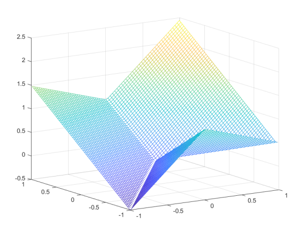
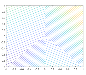
Figure 3: Mesh and Contour plot of the function from Eq. (8). Best viewed in color.

In a related direction, one might consider finding $\epsilon$-stationary points of other smooth approximations of the original function, which have a better behavior. For example, for nonconvex functions, a well-known smoothing operation with dimension-free guarantees is the Lasry-Lions regularization (Lasry and Lions, 1986; Attouch and Aze, 1993), which is closely related to the Moreau-Yosida regularization for smoothing convex functions. However, this operation does not appear to be efficiently computable in general.

Finally, it is important to step back and point out that when considering optimization of nonsmooth nonconvex functions, it is generally difficult to relate stationarity properties to any meaningful local optimality properties, even more so than in the smooth case. For example, consider the simple nonsmooth bivariate function studied in (Warga, 1981; Czarnecki and Rifford, 2006),

$$f(u,v)=\Big{|}\left|u\right|+v\Big{|}+\frac{1}{2}u~{},$$ (8)

which is illustrated in Fig. 3. It can be shown that the origin is a (Clarke) stationary point. However, it is not even approximately-stationary with respect to standard smooth approximations of the function, regardless of how tight we make them. Also, it is clearly not a point we would like our algorithm to converge to, if we actually try to minimize the function. This suggests looking for notions beyond stationarity, for which we can still provide algorithmic guarantees even for nonconvex nonsmooth functions.

Appendix A Proof of Thm. 2

In the proof, we let bold-faced letters (e.g., $\mathbf{x}$) denote vectors, and $x_{i}$ denote the $i$-th coordinate of the vector $\mathbf{x}$. Also, we let $\mathbf{e}_{1},\mathbf{e}_{2},\ldots$ denote the standard basis vectors.

Our proof will closely follow the analysis employed in Lan and Zhou [2018, Theorem 3] for a slightly different setting.

Fix an iteration budget $T$ and some dimension $d\geq T$. Let $A$ be the symmetric $d\times d$ tridiagonal matrix defined as

$$\forall 1\leq i<T~{}~{}~{}~{}~{}~{}~{}~{} A(i,i)=2~{},~{}A(i,i+1)=-1$$

$$\forall 1<i\leq T~{}~{}~{}~{}~{}~{}~{}~{} A(i,i-1)=-1$$

$$A(T,T)=k:=\frac{\sqrt{2}+3}{\sqrt{2}+1}$$

$$A(i,j)=0~{}~{}~{}\text{for all other $(i,j)$}~{}.$$

Also, for some constant $b$ to be determined later, define the quadratic function

$$g(\mathbf{x})~{}:=~{}\mathbf{x}^{\top}M\mathbf{x}-\frac{1}{4}\mathbf{e}_{1}^{\top}\mathbf{x}+b~{}~{}~{}\text{where}~{}~{}~{}M=\frac{1}{8}(A+4I)~{}.$$

It is easily verified that this function can be equivalently written as

$$g(\mathbf{x})~{}=~{}\frac{1}{8}\left(x_{1}^{2}+\sum_{i=1}^{T-1}(x_{i}-x_{i+1})^{2}+(k-1)x_{T}^{2}-2x_{1}\right)+\frac{1}{2}\|\mathbf{x}\|^{2}+b~{}.$$ (9)

We first collect a few useful facts about $g(\cdot)$, stated in the following two lemmas:

Lemma 4.

$M$ satisfies $\frac{1}{2}\leq\lambda_{\min}(M)\leq\lambda_{\max}(M)\leq 1$. As a result, $M$ is positive definite, and $g(\cdot)$ is strictly convex and has a unique minimum.

Proof.

$A$ is symmetric, and for any $\mathbf{x}\in\mathbb{R}^{T}$, we have

$$\mathbf{x}^{\top}A\mathbf{x}~{}=~{}x_{1}^{2}+\sum_{i=1}^{T-1}(x_{i}-x_{i+1})^{2}+(k-1)x_{T}^{2}~{}.$$

This is non-negative, which establishes that $A$ is a positive semidefinite matrix. Hence, by definition of $M$, $\lambda_{\min}(M)=\frac{1}{8}(\lambda_{\min}(A)+4)\geq\frac{1}{8}\cdot 4=\frac{1}{2}$, which implies that $M$ is positive definite. As a result, $g(\cdot)$ is strictly convex and has a unique minimum. Also, by the displayed equation above,

$$\mathbf{x}^{\top}A\mathbf{x}~{} \leq~{}x_{1}^{2}+2\sum_{i=1}^{T-1}(x_{i}^{2}+x_{i+1}^{2})+(k-1)x_{T}^{2}~{}\leq~{}3x_{1}^{2}+\sum_{i=2}^{T-1}(2x_{i}^{2}+2x_{i+1}^{2})+(k-1)x_{T}^{2}$$

$$=~{}3x_{1}^{2}+4\sum_{i=2}^{T-1}x_{i}^{2}+(k+1)x_{T}^{2}~{}\leq~{}4\|\mathbf{x}\|^{2}~{},$$

where we use the fact that $k\leq 3$. This establishes that $\lambda_{\max}(A)\leq 4$, and therefore $\lambda_{\max}(M)=\frac{1}{8}(\lambda_{\max}(A)+4)\leq 1$. ∎

Lemma 5.

The minimum $\mathbf{x}^{*}$ of $g(\cdot)$ is of the form $\mathbf{x}^{*}=(q,q^{2},\ldots,q^{T},0,\ldots,0)$, where $q=\frac{\sqrt{2}-1}{\sqrt{2}+1}$. Moreover, $\|\mathbf{x}^{*}\|\leq\sqrt{\frac{\sqrt{2}-1}{2}}<\frac{1}{2}$.

Proof.

By the previous lemma and the fact that $g(\cdot)$ is differentiable, $\mathbf{x}^{*}$ is the unique point satisfying $\nabla g(\mathbf{x}^{*})=\mathbf{0}$. Thus, it is enough to verify that the formula for $\mathbf{x}^{*}$ stated in the lemma indeed satisfies this equation. Computing the gradient of $g(\cdot)$ using the formulation in Eq. (9)), we just need to verify that

$$6q-q^{2}-1=0~{}~{},~{}~{}\forall i\in\{2,\ldots,T-1\}~{}~{}q^{i-1}-6q^{i}+q^{i+1}=0~{}~{},~{}~{}(k+4)q^{T}-q^{T-1}=0~{},$$

or equivalently,

$$1-6q+q^{2}=0~{}~{},~{}~{}(k+4)q-1=0~{},$$

which is easily verified to hold for the value of $q$ stated in the lemma. Finally, we have

$$\|\mathbf{x}^{*}\|^{2}=\sum_{i=1}^{d}(x^{*}_{i})^{2}=\sum_{i=1}^{T}q^{i}<\sum_{i=1}^{\infty}q^{i}~{}=~{}\frac{q}{1-q}=\frac{\sqrt{2}-1}{2},$$

implying $\|\mathbf{x}^{*}\|\leq\sqrt{\frac{\sqrt{2}-1}{2}}$ as required. ∎

Finally, we assume that the constant term $b$ in Eq. (9) is fixed so that $g(\mathbf{x}^{*})=0$, which means that $g(\cdot)$ can be written in the form

$$g(\mathbf{x})~{}=~{}(\mathbf{x}-\mathbf{x}^{*})^{\top}M(\mathbf{x}-\mathbf{x}^{*})~{}.$$ (10)

With this construction in hand, we now turn to prove the theorem. We will start with the family of linear-span algorithms $\mathcal{A}_{span}$, using any dimension $d\geq T$, and take $g(\cdot)$ as the “hard” function on which we will prove a lower bound (note that by the lemmas above and Eq. (10), it satisfies the conditions stated in the theorem).

Consider any algorithm in $\mathcal{A}_{span}$, and note that by the structure of $g(\cdot)$ as specified in Eq. (9), when the algorithm picks its first query $\mathbf{x}_{1}=\mathbf{0}$, it receives a gradient in $\text{span}\{\mathbf{e}_{1}\}$. Because of the linear-span assumption, it means that $\mathbf{x}_{2}\in\text{span}(\mathbf{e}_{1})$, which again by Eq. (9) means that the returned gradient is in $\text{span}\{\mathbf{e}_{1},\mathbf{e}_{2}\}$. Continuing this process, it is easily seen by induction that

$$\mathbf{x}_{t}\in\text{span}\left\{\mathbf{e}_{1},\ldots,\mathbf{e}_{t-1}\right\}$$

for all $t$, and in particular, $\{\mathbf{x}_{1},\ldots,\mathbf{x}_{T}\}\subset\text{span}\left(\mathbf{e}_{1},\ldots,\mathbf{e}_{T-1}\right)$. As a result,

$$\min_{t\in\{1,\ldots,T\}}\|\mathbf{x}_{t}-\mathbf{x}^{*}\|^{2}~{}\geq~{}\inf_{\mathbf{x}\in\text{span}\{\mathbf{e}_{1},\ldots,\mathbf{e}_{T-1}\}}\|\mathbf{x}_{t}-\mathbf{x}^{*}\|^{2}~{}\geq~{}(x_{T}^{*})^{2},$$

which by Lemma 5 is at least $q^{2T}=\left(\frac{\sqrt{2}-1}{\sqrt{2}+1}\right)^{2T}$. Taking a square root, we get that

$$\min_{t\in\{1,\ldots,T\}}\|\mathbf{x}_{t}-\mathbf{x}^{*}\|~{}\geq~{}\left(\frac{\sqrt{2}-1}{\sqrt{2}+1}\right)^{T}~{}\geq~{}\exp(-T)~{},$$

as stated in the theorem.

We now turn to prove the theorem for deterministic algorithms. This time, we will let the dimension be any $d\geq 2T$. Fixing an algorithm, and letting $\mathbf{u}_{1},\ldots,\mathbf{u}_{T}$ be orthonormal vectors to be specified shortly, we prove the lower bound for the function

$$\tilde{g}(\mathbf{x})~{}:=~{}\frac{1}{8}\left((\mathbf{u}_{1}^{\top}\mathbf{x})^{2}+\sum_{i=1}^{T-1}(\mathbf{u}_{i}^{\top}\mathbf{x}-\mathbf{u}_{i+1}^{\top}\mathbf{x})^{2}+(k-1)(\mathbf{u}_{T}^{\top}\mathbf{x})^{2}-2\mathbf{u}_{1}^{\top}\mathbf{x}\right)+\frac{1}{2}\|\mathbf{x}\|^{2}+b~{}.$$ (11)

Importantly, we note that

$$\tilde{g}(\mathbf{x})~{}=~{}g(U\mathbf{x})$$

where $g(\cdot)$ is the function defined previously in Eq. (9), and $U$ is an orthogonal matrix whose first $T$ rows are $\mathbf{u}_{1},\ldots,\mathbf{u}_{T}$, and the rest of the rows are some arbitrary completion of the first $T$ rows to an orthonormal basis. Thus, $\tilde{g}(\cdot)$ is equivalent to $g(\cdot)$ up to a rotation of the coordinate system specified by $U$. In particular, using Eq. (10), it follows that

$$\tilde{g}(\mathbf{x})~{} =~{}(U\mathbf{x}-\mathbf{x}^{*})^{\top}M(U\mathbf{x}-\mathbf{w}^{*})~{}=~{}(\mathbf{x}-U^{\top}\mathbf{x}^{*})^{\top}(U^{\top}MU)(\mathbf{x}-U^{\top}\mathbf{x}^{*})$$

$$=~{}(\mathbf{x}-\tilde{\mathbf{x}}^{*})^{\top}\tilde{M}(\mathbf{x}-\tilde{\mathbf{x}}^{*})~{},$$

where $\tilde{M}=U^{\top}MU$ and $\tilde{\mathbf{x}}^{*}=U^{\top}\mathbf{x}^{*}$. Thus, we see that $\tilde{g}(\cdot)$ has the form required in the theorem, with a matrix $\tilde{M}$ whose spectrum is identical to $M$, and a minimizer $\tilde{\mathbf{x}}^{*}=U^{\top}\mathbf{x}^{*}$ whose norm is the same as $\|\mathbf{x}^{*}\|$ (and therefore satisfying the conditions in the theorem).

We now specify how to choose $\mathbf{u}_{1},\ldots,\mathbf{u}_{T}$ in the function definition, so as to get the lower bound on $\min_{t}\|\mathbf{x}_{t}-\tilde{\mathbf{x}}^{*}\|$: Since the algorithm is deterministic, its first query point $\mathbf{x}_{1}$ is known in advance. We therefore choose $\mathbf{u}_{1}$ to be some unit vector orthogonal to $\mathbf{x}_{1}$. Assuming that $\mathbf{u}_{2},\mathbf{u}_{3},\ldots$ are orthogonal to $\{\mathbf{u}_{1},\mathbf{x}_{1}\}$ (which we shall justify shortly), we have by Eq. (11) that $\tilde{g}(\mathbf{x}_{1})$ and $\nabla\tilde{g}(\mathbf{x}_{1})$ depend only on $\mathbf{x}_{1},\mathbf{u}_{1}$, and not on $\mathbf{u}_{2},\mathbf{u}_{3},\ldots$. As the algorithm is deterministic and depends only on the observed values and gradients, this means that even before choosing $\mathbf{u}_{2},\mathbf{u}_{3},\ldots$, we can already simulate its next iteration, and determine the next query point $\mathbf{x}_{2}$. We now pick $\mathbf{u}_{2}$ to be some unit vector orthogonal to $\mathbf{u}_{1}$ as well as to $\mathbf{x}_{1},\mathbf{x}_{2}$. Again by the same considerations, if we assume $\mathbf{u}_{3},\mathbf{u}_{4},\ldots$ are orthogonal to $\{\mathbf{u}_{i},\mathbf{x}_{i}\}_{i=1}^{2}$, we have that $\tilde{g}(\mathbf{x}_{2})$ and $\nabla\tilde{g}(\mathbf{x}_{2})$ depend only on $\{\mathbf{u}_{i},\mathbf{x}_{i}\}_{i=1}^{2}$, and independent of $\mathbf{u}_{3},\mathbf{u}_{4},\ldots$. So again, we can simulate it and determine the next query point $\mathbf{x}_{3}$. We continue this process up to iteration $T$, where we fix $\mathbf{u}_{T}$ orthogonal to $\{\mathbf{u}_{i},\mathbf{x}_{i}\}_{i=1}^{T-1}$ and to $\mathbf{x}_{T}$ (this process is possible as long as the dimension $d$ is at least $2(T-1)+1+1=2T$, as we indeed assume).

As a result of this process, we get that $\mathbf{u}_{T}^{\top}\mathbf{x}_{t}=0$ for all $t\in\{1,\ldots,T\}$. Also, since $\tilde{\mathbf{x}}^{*}=U^{\top}\mathbf{x}^{*}$, we also have $\mathbf{u}_{T}^{\top}\tilde{\mathbf{x}}^{*}=\mathbf{u}_{T}^{\top}U^{\top}\tilde{\mathbf{x}}^{*}=x_{T}^{*}$. Using Lemma 5, we get that for all $t\in\{1,\ldots,T\}$,

$$\|\mathbf{x}_{t}-\tilde{\mathbf{x}}^{*}\|^{2}\geq(\mathbf{u}_{T}^{\top}(\mathbf{x}_{t}-\tilde{\mathbf{x}}^{*}))^{2}~{}=~{}(0-x_{T}^{*})^{2}=\left(\frac{\sqrt{2}-1}{\sqrt{2}+1}\right)^{2T}~{},$$

which implies that

$$\min_{t\in\{1,\ldots,T\}}\|\mathbf{x}_{t}-\mathbf{x}^{*}\|~{}\geq~{}\left(\frac{\sqrt{2}-1}{\sqrt{2}+1}\right)^{T}~{}\geq~{}\exp(-T)$$

as required.

References

- Arjevani et al. [2019] Yossi Arjevani, Ohad Shamir, and Ron Shiff. Oracle complexity of second-order methods for smooth convex optimization. Mathematical Programming, 178(1-2):327–360, 2019.
- Attouch and Aze [1993] Hédy Attouch and Dominique Aze. Approximation and regularization of arbitrary functions in hilbert spaces by the lasry-lions method. In Annales de l’Institut Henri Poincare (C) Non Linear Analysis, volume 10, pages 289–312. Elsevier, 1993.
- Beck and Hallak [2020] Amir Beck and Nadav Hallak. On the convergence to stationary points of deterministic and randomized feasible descent directions methods. SIAM Journal on Optimization, 30(1):56–79, 2020.
- Benaïm et al. [2005] Michel Benaïm, Josef Hofbauer, and Sylvain Sorin. Stochastic approximations and differential inclusions. SIAM Journal on Control and Optimization, 44(1):328–348, 2005.
- Bolte et al. [2018] Jérôme Bolte, Shoham Sabach, Marc Teboulle, and Yakov Vaisbourd. First order methods beyond convexity and lipschitz gradient continuity with applications to quadratic inverse problems. SIAM Journal on Optimization, 28(3):2131–2151, 2018.
- Carmon et al. [2019] Yair Carmon, John C Duchi, Oliver Hinder, and Aaron Sidford. Lower bounds for finding stationary points i. Mathematical Programming, pages 1–50, 2019.
- Clarke [1990] Frank H Clarke. Optimization and nonsmooth analysis, volume 5. Siam, 1990.
- Czarnecki and Rifford [2006] Marc-Olivier Czarnecki and Ludovic Rifford. Approximation and regularization of lipschitz functions: convergence of the gradients. Transactions of the American Mathematical Society, 358(10):4467–4520, 2006.
- Davis and Drusvyatskiy [2019] Damek Davis and Dmitriy Drusvyatskiy. Stochastic model-based minimization of weakly convex functions. SIAM Journal on Optimization, 29(1):207–239, 2019.
- Davis et al. [2018] Damek Davis, Dmitriy Drusvyatskiy, Sham Kakade, and Jason D Lee. Stochastic subgradient method converges on tame functions. Foundations of computational mathematics, pages 1–36, 2018.
- Drusvyatskiy and Paquette [2019] Dmitriy Drusvyatskiy and Courtney Paquette. Efficiency of minimizing compositions of convex functions and smooth maps. Mathematical Programming, 178(1-2):503–558, 2019.
- Duchi and Ruan [2018] John C Duchi and Feng Ruan. Stochastic methods for composite and weakly convex optimization problems. SIAM Journal on Optimization, 28(4):3229–3259, 2018.
- Duchi et al. [2012] John C Duchi, Peter L Bartlett, and Martin J Wainwright. Randomized smoothing for stochastic optimization. SIAM Journal on Optimization, 22(2):674–701, 2012.
- Ghadimi and Lan [2013] Saeed Ghadimi and Guanghui Lan. Stochastic first-and zeroth-order methods for nonconvex stochastic programming. SIAM Journal on Optimization, 23(4):2341–2368, 2013.
- Goldstein [1977] AA Goldstein. Optimization of lipschitz continuous functions. Mathematical Programming, 13(1):14–22, 1977.
- Jin et al. [2017] Chi Jin, Rong Ge, Praneeth Netrapalli, Sham M Kakade, and Michael I Jordan. How to escape saddle points efficiently. In Proceedings of the 34th International Conference on Machine Learning-Volume 70, pages 1724–1732. JMLR. org, 2017.
- Kiwiel [2007] Krzysztof C Kiwiel. Convergence of the gradient sampling algorithm for nonsmooth nonconvex optimization. SIAM Journal on Optimization, 18(2):379–388, 2007.
- Lan and Zhou [2018] Guanghui Lan and Yi Zhou. An optimal randomized incremental gradient method. Mathematical programming, 171(1-2):167–215, 2018.
- Lasry and Lions [1986] Jean-Michel Lasry and Pierre-Louis Lions. A remark on regularization in hilbert spaces. Israel Journal of Mathematics, 55(3):257–266, 1986.
- Majewski et al. [2018] Szymon Majewski, Błażej Miasojedow, and Eric Moulines. Analysis of nonsmooth stochastic approximation: the differential inclusion approach. arXiv preprint arXiv:1805.01916, 2018.
- Nemirovsky and Yudin [1983] Arkadii Semenovich Nemirovsky and David Borisovich Yudin. Problem complexity and method efficiency in optimization. Wiley, 1983.
- Nesterov [2012] Yurii Nesterov. How to make the gradients small. Optima. Mathematical Optimization Society Newsletter, (88):10–11, 2012.
- Nesterov [2018] Yurii Nesterov. Lectures on convex optimization, volume 137. Springer, 2018.
- Simchowitz [2018] Max Simchowitz. On the randomized complexity of minimizing a convex quadratic function. arXiv preprint arXiv:1807.09386, 2018.
- Tkocz [2012] Tomasz Tkocz. An upper bound for spherical caps. The American Mathematical Monthly, 119(7):606–607, 2012.
- Warga [1981] Jack Warga. Fat homeomorphisms and unbounded derivate containers. Journal of Mathematical Analysis and Applications, 81(2):545–560, 1981.
- Woodworth and Srebro [2017] Blake Woodworth and Nathan Srebro. Lower bound for randomized first order convex optimization. arXiv preprint arXiv:1709.03594, 2017.
- Zhang et al. [2020] Jingzhao Zhang, Hongzhou Lin, Suvrit Sra, and Ali Jadbabaie. On complexity of finding stationary points of nonsmooth nonconvex functions. arXiv preprint arXiv:2002.04130, 2020.