On de Sitter future-past extremal surfaces
and the “entanglement wedge”

K. Narayan

Chennai Mathematical Institute,
H1 SIPCOT IT Park, Siruseri 603103, India.

We develop further the codim-2 future-past extremal surfaces stretching between the future and past boundaries in de Sitter space, discussed in previous work. We first make more elaborate the construction of such surfaces anchored at more general subregions of the future boundary, and stretching to equivalent subregions at the past boundary. These top-bottom symmetric future-past extremal surfaces cannot penetrate beyond a certain limiting surface in the Northern/Southern diamond regions: the boundary subregions become the whole boundary for this limiting surface. For multiple disjoint subregions, this construction leads to mutual information vanishing and strong subadditivity being saturated. We then discuss an effective codim-1 envelope surface arising from these codim-2 surfaces. This leads to analogs of the entanglement wedge and subregion duality for these future-past extremal surfaces in de Sitter space.

1 Introduction

de Sitter space is of great interest for various reasons: theoretically there is the striking fact that it has thermodynamic properties, with temperature and entropy [2] (see the review [3]). This entropy arises as the area of the cosmological horizon in the static patch coordinatization for observers in the Northern/Southern diamond regions who view these as event horizons. It is fascinating to ask how de Sitter entropy can be understood via gauge/gravity duality [4, 5, 6, 7] for de Sitter space, or $dS/CFT$ [8, 9, 10], which associates a hypothetical non-unitary dual Euclidean CFT at the future boundary $I^{+}$, which might be regarded as the natural boundary of de Sitter space (see e.g. [11]). The $dS/CFT$ dictionary $\Psi_{dS}=Z_{CFT}$ [10], with $\Psi_{dS}$ is the late-time Hartle-Hawking Wavefunction of the Universe with appropriate boundary conditions and $Z_{CFT}$ the dual CFT partition function, is quite different from $Z_{bulk}=Z_{CFT}$ in the $AdS$ case. For instance, for $dS_{4}$, we have (semiclassically)

$$\qquad\qquad\qquad\quad Z_{{}_{CFT}}=\Psi_{{}_{dS}}\sim e^{iS_{cl}}\sim e^{-\int_{k}R_{dS}^{2}k^{3}\varphi_{-k}^{0}\varphi_{k}^{0}\,+\,\ldots}\ ,$$

$$\langle O_{k}O_{k^{\prime}}\rangle\sim{\delta^{2}Z_{{}_{CFT}}\over\delta\varphi_{k}^{0}\delta\varphi_{k^{\prime}}^{0}}\ ,\qquad\quad\langle\varphi_{k}\,\varphi_{k^{\prime}}\rangle\sim\int D\varphi\ \varphi_{k}\,\varphi_{k^{\prime}}\,\big{|}\Psi_{dS}[\varphi_{k}]\big{|}^{2}\ .$$ (1)

The $CFT_{d}$ energy momentum tensor 2-point correlation functions yield central charges that are negative or imaginary (odd dimensions), effectively analytic continuations from $AdS$: e.g. taking $O_{k}$ as appropriate $T_{ij}$ components gives the real, negative, central charge $-{R_{dS}^{2}\over G_{4}}$  reminiscent of ghost-like ($c<0$) theories. In [12], a higher spin $dS_{4}$ duality was conjectured involving a 3-dim CFT of anti-commuting (ghost) scalars, which exemplifies this (see also e.g. [13]-[21]). While dual operator correlation functions are obtained by a differentiate prescription applied to $Z_{CFT}$, bulk expectation values are obtained by weighting with the bulk probability $|\Psi_{dS}|^{2}$. The fact that bulk observables in this formulation require both $\Psi_{dS}$ and $\Psi_{dS}^{*}$ suggests that two copies of the dual CFT are required for a fixed $dS$ background (strictly one should also sum over final 3-metrics in $|\Psi_{dS}[\varphi,g^{3}]|^{2}$).

In this context it is interesting to ask if the various ideas and techniques pertaining to holographic entanglement unravelled in $AdS/CFT$ [22, 23, 24] (reviewed in e.g. [25, 26, 27]) have analogs in de Sitter space, perhaps leading to insights into de Sitter entropy as some sort of generalized entanglement entropy. In the $AdS$ case, the areas of extremal surfaces anchored at the boundary of subsystems in the boundary theory encode the entanglement entropy of the subsystem in the dual field theory. It is known that $AdS$ is special in many ways: many apparently gravitational or geometric quantities are actually field theory quantities. For instance, the extremal surfaces encoding entanglement are geometric objects but very strikingly they automatically satisfy the various inequalities that entanglement entropy in field theory is required to satisfy. In these cases, the dual field theory includes the time direction. It is thus not clear if any of these ideas and mathematical formulations of entanglement make sense away from $AdS/CFT$, or more generally gauge/gravity duality for ordinary field theories. In de Sitter, the natural boundary is at (future or past) timelike infinity and is spatial so the dual is hypothesised to be a Euclidean nonunitary CFT.

One way to set up the analog of the Ryu-Takayanagi formulation in $dS$, for one thing simply as a geometric problem, is to look for extremal surfaces pertaining to subregions at the future boundary (see [28] for a review of these investigations). Since the theory is Euclidean, there is no natural time direction: as a calculational crutch, one could pick one of the spatial symmetry directions as boundary Euclidean time and look for extremal surfaces on bulk slices corresponding to these. All such slices must be equivalent however since none of these is sacrosanct. In the Poincare slicing, this exercise shows that surfaces that begin at $I^{+}$ do not turn back somewhere in the bulk to return to $I^{+}$: there is no real turning point for such timelike surfaces ending on the spatial boundary. There are complex extremal surfaces with turning points, amounting to analytic continuation from the $AdS$ Ryu-Takayanagi surfaces but their interpretation is unclear.

In [29], certain codim-2 timeline extremal surfaces were found stretching from the future boundary to the past: this is perhaps natural given that surfaces do not return to $I^{+}$, so they could instead end at $I^{-}$. This also dovetails with the fact that bulk expectation values require two copies of the wavefunction and so two CFT copies and therefore two boundaries. These surfaces begin at $I^{+}$, the future boundary of the future universe $F$, have a turning point in the Northern/Southern diamond regions $N/S$ and then end at the past boundary $I^{-}$ of the past universe $P$. These are analogous to rotated versions of the surfaces discussed by Hartman, Maldacena [30] in the eternal $AdS$ black hole. It turns out that these surfaces cannot penetrate into the Northern/Southern diamond regions $N/S$ beyond a certain point (for $dS_{4}$ and higher dimensions): the turning point has a real-valued solution only for certain subregions of $N/S$. The limiting surface arises as the subregion at $I^{\pm}$ becomes the whole space (this limit was identified erroneously in [29]).

These surfaces turn out to have various interesting properties, as we will explore in this paper. We restrict attention to “top-bottom symmetric” surfaces, stretching between a subregion ${\cal A}\in I^{+}$ and an equivalent subregion at $I^{-}$: this in some sense simulates the bulk inner product $\Psi^{*}_{I^{+}}{\cal O}\Psi_{I^{+}}$ in (1), with $\Psi_{I^{-}}\equiv\Psi_{I^{+}}^{*}$ . First we will make more elaborate (sec. 2) the construction of these extremal surfaces for more general subregions, as well as discuss the limiting surface in more detail. This construction shows that for multiple disjoint subregions, mutual information vanishes and strong subadditivity is saturated. This is reminiscent of finite temperature systems in $AdS/CFT$, and is perhaps consistent with the fact that the bulk de Sitter spacetime has a temperature. We then argue that there is an effective codim-1 envelope surface formed from the union or envelope of all the codim-2 surfaces. This leads to analogs of the entanglement wedge (sec. 3) and a version of subregion duality, adapting to this de Sitter case the various arguments on the entanglement wedge in $AdS/CFT$ [31, 32, 33]. We close with a Discussion (sec. 4).

2 de Sitter space and future-past extremal surfaces

In $AdS$, surfaces starting at the boundary dip into the radial direction and exhibit turning points where they begin to return to the boundary. In $dS$, the boundary at $I^{+}$ is spatial: surfaces dip into the time direction (which is holographic) giving a crucial minus sign that ensures that there is no real turning point where the surface starting at $I^{+}$ begins to turn back towards $I^{+}$ [34, 35]. For instance, in the Poincare slicing $ds^{2}={R_{dS}^{2}\over\tau^{2}}(-d\tau^{2}+dx_{i}^{2})$ , a strip subsystem on some boundary Euclidean time $w=const$ slice of $I^{+}$ with width along $x$ gives a bulk extremal surface $x(\tau)$ described by ${\dot{x}}^{2}\equiv({dx\over d\tau})^{2}={B^{2}\tau^{2d-2}\over 1+B^{2}\tau^{2d-2}}$ ($B^{2}>0$). $w$, $x$ can be any of the $x_{i}$ (no boundary Euclidean time slice is special). A turning point where the surface starting at $I^{+}$ begins to turn back requires $|{\dot{x}}|\rightarrow\infty$ while here $|{\dot{x}}|\leq 1$. If such a turning point existed, the extremal surface, initially dipping into the bulk time direction (so that $|{dw\over d\tau}|<1$), would have to stop moving in time and hit $|{dw\over d\tau}|\rightarrow\infty$ which is a spacelike condition. Thus the surface needs to transit from being timelike to being spacelike and then again timelike: this appears incompatible with the extremality of the surface, which is taken to be smooth. (There are also complex extremal surfaces with turning points, amounting to analytic continuation from the $AdS$ Ryu-Takayanagi surfaces [34, 35, 36, 37]: their interpretation is unclear, the time parameter taking imaginary time paths, thus lying outside the original de Sitter time parametrization.)

Since real surfaces starting at the future boundary $I^{+}$ keep marching on into the bulk without returning, it is interesting to ask if they could instead end at the past boundary $I^{-}$ [29]. The bulk probability $\Psi_{dS}^{*}\Psi_{dS}$ suggests two CFT copies: so such connected extremal surfaces stretching between $I^{\pm}$ are perhaps expected. Towards studying this, we recast $dS_{d+1}$ in the static coordinatization $ds^{2}=-(1-r^{2}/l^{2})dt^{2}+{dr^{2}\over 1-r^{2}/l^{2}}+r^{2}d\Omega_{d-1}^{2}$ as

$$ds^{2}_{d+1}={l^{2}\over\tau^{2}}\left(-{d\tau^{2}\over 1-\tau^{2}}+(1-\tau^{2})dw^{2}+d\Omega_{d-1}^{2}\right),$$ (2)

where $\tau={l\over r}\ w={t\over l}$. Now $\tau$ is “bulk” time: $0\leq\tau\leq 1$ define the future-past universes $F/P$ while the Northern/Southern diamond regions $N/S$ have $1<\tau\leq\infty$ (with $w$ time). There are horizons at $\tau=1$: their area is ${\pi l^{2}\over G_{4}}$ . The boundary at $\tau\sim 0$ is Euclidean $R_{w}\times S^{d-1}$.

Since the asymptotic region enjoys rotational invariance in $S^{d-1}$ as well as $w$-translations, we could pick either some equatorial plane of the $S^{d-1}$ or a $w=const$ slice as a boundary Euclidean time slice. The area functional for a codim-2 surface on an $S^{d-1}$ equatorial plane is

$$S=\ l^{d-1}V_{S^{d-2}}\int{d\tau\over\tau^{d-1}}\sqrt{{1\over 1-\tau^{2}}-(1-\tau^{2})(w^{\prime})^{2}}\ .$$ (3)

Such codim-2 extremal surfaces are consistent with the scaling ${l^{d-1}\over G_{d+1}}$ of de Sitter entropy. (The $w=const$ slice turns out to be difficult to analyse in detail, although certain aspects such as the leading divergence are straightforward to see.) Extremizing this gives the surface equation and its area as

$${\dot{w}}^{2}\equiv(1-\tau^{2})^{2}\Big{(}{dw\over d\tau}\Big{)}^{2}={B^{2}\tau^{2d-2}\over 1-\tau^{2}+B^{2}\tau^{2d-2}}\ ,\quad S={2l^{d-1}V_{S^{d-2}}\over 4G_{d+1}}\int_{\epsilon}^{\tau_{*}}{d\tau\over\tau^{d-1}}\ {1\over\sqrt{1-\tau^{2}+B^{2}\tau^{2d-2}}}\ .$$ (4)

Here ${\dot{w}}$ is the $y$-derivative, with

$$y=\int{d\tau\over 1-\tau^{2}}={1\over 2}\log\Big{|}{1+\tau\over 1-\tau}\Big{|}$$ (5)

the “tortoise” coordinate, useful near the horizons. The turning point is the “deepest” location to which the surface dips into in the bulk, before turning around: this is given by

$$|{\dot{w}}|\rightarrow\infty:\qquad\ 1-\tau_{*}^{2}+B^{2}\tau_{*}^{2d-2}\ =\ 0\ .$$ (6)

With $B^{2}>0$, real $\tau_{*}(B^{2})$ arises only if $\tau>1$ i.e. within $N/S$. For any finite $B^{2}>0$, we have ${\dot{w}}\rightarrow 0^{+}$ near $\tau\rightarrow 0$, with ${\dot{w}}<1$ for $\tau<1$ (within $F$) and ${\dot{w}}\rightarrow 1$ as $\tau\rightarrow 1$. Overall this gives the smooth “hourglass”-like red curve in Figure 1 representing the codim-2 extremal surface stretching from a subregion $\Delta w\times S^{d-2}$ at $I^{+}$ to an equivalent one at $I^{-}$, intersecting the horizons, turning around smoothly at $\tau_{*}$ in $N$/$S$. The full extremal surface for the subregion consists of the left and right portions of the surface. We will discuss this more elaborately in what follows.

2.1 Future-past extremal surfaces for general subregions

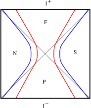
Figure 1: Future-past extremal surfaces in de Sitter stretching between $I^{\pm}$. These are akin to rotated Hartman-Maldacena
surfaces in the eternal $AdS$ black hole. The red curve is for
generic subregion. The blue curve is a limiting curve obtained
as the subregion becomes the whole space.

We would like to construct these future-past extremal surfaces for general subregions at $I^{\pm}$, restricting however to surfaces which are top-bottom symmetric: as we have stated, this in some sense simulates the bulk inner product (1). In other words, the surface is symmetric about the $w=0$ slice passing horizontally through the middle of the Penrose diagram, i.e. the top half-surface (anchored at $I^{+}$) is identical pictorially to the bottom half-surface (anchored at $I^{-}$); see Figure 1. To describe these explicitly, consider any $S^{d-1}$ equatorial plane and a subregion at $I^{+}$ defined as

$${\cal A}\equiv(w_{L,0},w_{R,0})\ ,\qquad w_{R,0}>w_{L,0}\ ,$$ (7)

where $w_{R,0}$ is the “right” edge and $w_{L,0}$ is the “left” edge of the subregion at $I^{+}$. We take the convention that $I^{+}$ is parametrized by $w$ with the “left” end being $w\rightarrow-\infty$ and the “right” end being $w\rightarrow\infty$ (see e.g. [3]). Then $I^{-}$ is parametrized with $w\rightarrow\infty$ at the “left” end and $w\rightarrow-\infty$ at the right end (the flow of $\partial_{w}$ is reversed). This dovetails with taking $w_{R,0}>w_{L,0}$. To be concrete, consider first the subregion in Figure 1, which is also left-right symmetric (we will consider more general subregions later). The full future-past surface is defined by two sets of equations, one for the top half-surface (anchored in the future universe) and the other for the bottom half-surface (anchored in the past universe),

$$top:\quad w_{L}(y)=w_{L,0}-\int_{0}^{y}dy\,{\dot{w}_{L}}(B_{L})\,;\qquad w_{R}(y)=w_{R,0}+\int_{0}^{y}dy\,{\dot{w}_{R}}(B_{R})\,,$$

$$bottom:\quad w_{L}(y)=-w_{L,0}+\int_{0}^{y}dy\,{\dot{w}_{L}}(B_{L})\,;\qquad w_{R}(y)=-w_{R,0}-\int_{0}^{y}dy\,{\dot{w}_{R}}(B_{R})\,,\ \$$ (8)

with ${\dot{w}_{L}}(B_{L})$ and ${\dot{w}_{R}}(B_{R})$ given by (4), taking the positive square root, with parameters $B_{L}$ and $B_{R}$ respectively. The top and bottom half-surfaces are reflections of each other about the $w=0$ slice: i.e. the bottom surface is obtained from the top one as $w(y)\rightarrow-w(y)$. The parameters $B_{L},B_{R}$ are related to the turning points (6) of the surfaces $w_{L}(y)$ and $w_{R}(y)$ as

$$1-\tau_{*,L}^{2}+B_{L}^{2}\tau_{*,L}^{4}=0\ ,\qquad 1-\tau_{*,R}^{2}+B_{R}^{2}\tau_{*,R}^{4}=0\ ;\qquad\tau_{*,L,R}={e^{2y_{*,L,R}}+1\over e^{2y_{*,L,R}}-1}\ .$$ (9)

The turning points lie in the $N/S$ regions as stated earlier, so we have used the corresponding expressions for $\tau_{*}(y)$ using (5). The figure is top-bottom symmetric, as are the extremal surfaces as we have stated. Thus the turning points lie on the $w=0$ slice: so we have for the top half-surface (using (2.1))

$$0=w_{L}(y_{*,L})=w_{L,0}-\int_{0}^{y_{*,L}}dy\,{\dot{w}_{L}}(B_{L})\ ,\qquad 0=w_{R}(y_{*,R})=w_{R,0}+\int_{0}^{y_{*,R}}dy\,{\dot{w}_{R}}(B_{R})\ ,$$ (10)

which are also automatically satisfied for the bottom half-surface. This gives a relation between the boundary conditions at $I^{\pm}$, the turning points and the parameters $B$,

$$w_{L,0}=\int_{0}^{y_{*,L}}dy\,{\dot{w}_{L}}(B_{L})\ ,\qquad w_{R,0}=-\int_{0}^{y_{*,R}}dy\,{\dot{w}_{R}}(B_{R})\ .$$ (11)

In other words, the boundary condition $w_{L,0}$ at $I^{+}$ implies a turning point at a specific location $\tau_{*,L}$ (and likewise for the right side surface): the bottom part of the left surface can join smoothly to the top part only if its turning point matches with that of the top part, which in turn implies that $w_{L,0}$ for the bottom part should match appropriately with the top part. This is why $w^{bottom}_{0}=-w^{top}_{0}$, as we have taken in defining the top and bottom half-surfaces (2.1). In the vicinity of the turning point, we have $w(\tau)\sim\pm\sqrt{\tau_{*}-\tau}$ for the top part of the surface: this joins smoothly with $w(\tau)\sim\mp\sqrt{\tau_{*}-\tau}$ from the bottom part of the surface. It can now be shown that the integral $\int_{0}^{y_{*}}dy\,{\dot{w}}$ in fact takes negative values: we will see this explicitly in a special case later, and it can also be checked numerically. Given this, we see from (11) that

$$w_{L,0}<0\ ,\qquad w_{R,0}>0\ ,$$ (12)

for the surface of the form (2.1) above: this has the left and right parts on the left and right halves of $I^{+}$ respectively, as for the left-right symmetric subregion with the red curves in Figure 1. As we see from (2.1), such a future-past surface stretches from $w_{0}\in I^{+}$ to $-w_{0}\in I^{-}$, passing through the turning point at $w=0$. Then the size of a subregion $A$ (7) at $I^{+}$ is

$$\Delta w=w_{R,0}-w_{L,0}\ ,$$ (13)

where $w_{0}$’s are given by (11). For the left-right symmetric subregion in Figure 1, we have

$$w^{top}_{R,0}=-w^{top}_{L,0}\ ,\quad w^{bottom}_{R,0}=-w^{bottom}_{L,0};\quad{\rm and}\quad w^{top}_{R,0}=-w^{bottom}_{R,0}\ ,\quad w^{top}_{L,0}=-w^{bottom}_{L,0},$$ (14)

the last two relations following from top-bottom symmetry. Left-right symmetry also means ${\dot{w}_{L}}={\dot{w}_{R}}\equiv{\dot{w}}$ and so the size of the subregion becomes

$$\Delta w=-2\int_{0}^{y_{*}}dy\,{\dot{w}}\ ,$$ (15)

where $y_{*}$ refers to the turning point for both left and right parts of the surface, which are now symmetric. This subregion size at $I^{\pm}$ can be evaluated, using (4), as

$$\Delta w=-2\int_{0}^{y_{*}}dy\,{B\tau^{2}\over\sqrt{1-\tau^{2}+B^{2}\tau^{4}}}=-2\int_{0}^{y_{*}}dy\,{\dot{w}}=-2\int_{0}^{Y}dy\,{\dot{w}}\ -\ 2\int_{Y}^{y_{*}}dy\,{\dot{w}}\ ;\quad\tau=\tau(y).$$ (16)

In the last expression, we have broken up the integral into the contribution outside the horizon and that inside the horizon. Near the horizon, where $y\rightarrow\infty$, we have introduced a cutoff $Y$ to regulate the calculation. Now note that ${\dot{w}}\rightarrow 1$ near the horizon so the contribution near the horizon can be estimated as $\int_{Y}dy+\int^{Y}dy=Y-Y$, and the apparent divergence cancels: the near horizon contribution to $\Delta w$ is nonsingular. This can also be seen in the $\tau$-coordinates, where we regulate the near horizon region with a cutoff $T$ as $T=1-\varepsilon$ for $\tau<1$ and $T=1+\varepsilon$ for $\tau<1$: this gives $\int^{1-\varepsilon}{d\tau\over 1-\tau^{2}}+\int_{1+\varepsilon}{d\tau\over 1-\tau^{2}}\sim-\log\varepsilon-(-\log\varepsilon)$, which is smooth. For generic subregion, the surface equation $w(\tau)$ has a turning point at a single zero of the denominator: then near the turning point, we have $w(\tau)\sim\sqrt{\tau_{*}-\tau}$ from the contribution near the turning point which is finite. Thus for generic subregion, the width does not grow large but remains finite: this occurs for generic values of $0\leq B<{1\over 2}$ for $dS_{4}$ .

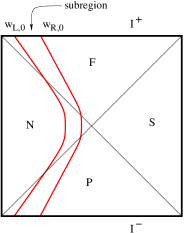
Figure 2: Future-past extremal surfaces in de Sitter
stretching between $I^{\pm}$ for a generic subregion: these lie
on some $S^{d-1}$ equatorial plane and have endpoints
$w_{L,0}$ at the left edge and $w_{R,0}$ at the right edge.

More generally, we see a relation between the equation describing a future-past surface and the corresponding boundary condition $w_{0}\in I^{+}$,

$$w(y)=w_{0}\mp\int_{0}^{y}dy\,{\dot{w}}(B)\qquad\Rightarrow\qquad w_{0}=\pm\int_{0}^{y_{*}}dy\,{\dot{w}}(B)\lessgtr 0\ ,$$ (17)

so that the top sign corresponds to a surface anchored in the left part of $I^{+}$ and the bottom sign to the right part of $I^{+}$. So consider e.g. the more general subregion and the red surfaces in Figure 2: this is top-bottom symmetric but not left-right symmetric. Now we have both $w_{L,0},w_{R,0}<0$ (with $w_{R,0}>w_{L,0}$): thus both surface equations $w_{L,R}(y)$ are of the form (17) with minus signs: explicitly

$$top:\qquad w_{L}(y)=w_{L,0}-\int_{0}^{y}dy\,{\dot{w}_{L}}(B_{L})\,;\qquad w_{R}(y)=w_{R,0}-\int_{0}^{y}dy\,{\dot{w}_{R}}(B_{R})\,,$$ (18)

with the bottom half-surfaces given by $w_{L}^{b}(y)=-w_{L}(y),\ w_{R}^{b}(y)=-w_{R}(y)$. The $B=0$ surface with ${\dot{w}}=0$ is a vertical line from $I^{+}$ to $I^{-}$, passing through the bifurcation point.

The full surface for a given subregion (7) consists of the left and right portions of the surface: the area is thus given by the sum of the areas

$$S[{\cal A}]=S[w_{L,0}]+S[w_{R,0}]$$ (19)

of the left and right portions of the surface, where each $S[w]$ is given by the area in (4). Each of the left and right portions of the surface of course connects the boundaries of the equivalent subregions at $I^{+}$ and $I^{-}$, but is disconnected from the other portion. The fact that the two sides of the full surface are disconnected from each other dovetails with the fact that a surface anchored at $I^{+}$ does not return to $I^{+}$ but ends at $I^{-}$. This disconnectedness has interesting consequences as we will see.

2.2 The limiting surface and its area

We will now see that the turning point relation (6) shows the existence of a limiting surface at some finite $\tau_{*}$ : these are shown as the blue curves in Figure 1. These future-past extremal surfaces cannot penetrate deeper than a certain location in the Northern/Southern diamond regions $N/S$ beyond the horizons: they are in some sense “repelled” by the poles (the left/right boundaries in $N/S$). This is analogous to the repulsive nature of the singularity with regard to the Hartman-Maldacena surfaces [30] in the eternal $AdS$ black hole.

From (6), we see that as $B\rightarrow 0$, we have $\tau_{*}\rightarrow 1$. On the other hand, we see that the expression cannot vanish if $\tau$ is too large: e.g. beyond $\tau_{*}^{2d-2}B^{2}\gtrsim\tau_{*}^{2}$, the two terms cannot cancel. This suggests a nontrivial solution around $\tau_{*}^{2d-4}\sim{1\over B^{2}}$. Focussing on $dS_{4}$, we can complete squares for $B\rightarrow{1\over 2}$ giving

$$[dS_{4}]\quad B\rightarrow{1\over 2}\,:\qquad 1-\tau^{2}+B^{2}\tau^{4}\ \rightarrow\ \Big{(}1-{\tau^{2}\over 2}\Big{)}^{2}\qquad\Rightarrow\qquad\tau_{*}\rightarrow\sqrt{2}\ ,$$ (20)

and the expression in (6) acquires a double zero. Now the width integral can acquire a logarithmic divergence: the surface is almost completely inside the horizon now (within the $N/S$ regions). Here we can approximate $\tau\gtrsim 1$ and so the subregion width (13), (15), can be approximated as

$$\Delta w\sim-2\int{d\tau\over\sqrt{1-\tau^{2}+B^{2}\tau^{4}}}\Big{|}_{\tau_{*}}$$ (21)

mostly arising from the contribution inside the horizon (ignoring finite constants). This is further vindicated since as we have seen above, the region near the horizon is smooth and the apparently divergent terms cancel after regulating. The subregion is becoming the whole space now, since $\Delta w\rightarrow\infty$ : the left and right edges are going to the boundaries of $I^{\pm}$.

To see all this more explicitly, we evaluate the width at this double zero location $B={1\over 2}$ . We have

$$\Delta w=-2\int_{0}^{1-\varepsilon}{d\tau\over 1-\tau^{2}}\,{\tau^{2}/2\over 1-\tau^{2}/2}-2\int_{1+\varepsilon}^{\sqrt{2}-\delta}{d\tau\over 1-\tau^{2}}\,{\tau^{2}/2\over 1-\tau^{2}/2}\ .$$ (22)

The $\varepsilon$ is related to the cutoff $Y$ mentioned earlier near the horizon (we are symmetrically “point-splitting” the horizon), while $\delta$ is a cutoff near the turning point $\tau_{*}=\sqrt{2}$ which will illustrate the logarithmic divergence. Noting ${1\over 1-\tau^{2}}\,{\tau^{2}/2\over 1-\tau^{2}/2}={1\over 1-\tau^{2}}-{2\over 2-\tau^{2}}$ , the integrals over $\tau<1$ and over $\tau>1$ are evaluated as

$$\tau<1:\qquad\int{d\tau\over 1-\tau^{2}}\,{\tau^{2}/2\over 1-\tau^{2}/2}={1\over 2}\log{1+\tau\over 1-\tau}+{1\over\sqrt{2}}\log{\sqrt{2}-\tau\over\sqrt{2}+\tau}\ ,$$

$$\tau>1:\qquad-\int{d\tau\over\tau^{2}-1}\,{\tau^{2}/2\over 1-\tau^{2}/2}={1\over 2}\log{1+\tau\over\tau-1}+{1\over\sqrt{2}}\log{\sqrt{2}-\tau\over\sqrt{2}+\tau}\ .$$ (23)

Then evaluating (22) vindicates the statements after (16) on the near horizon cutoff, giving

$$\Delta w = -\left(\log{1\over\varepsilon}+\log 2+\sqrt{2}\log{\sqrt{2}-1\over\sqrt{2}+1}\right)-\left(\log{\sqrt{2}+1\over\sqrt{2}-1}+\sqrt{2}\log{\delta\over 2\sqrt{2}}-\log{1\over\varepsilon}\right)$$ (24)

$$\sim \sqrt{2}\log{1\over\delta}\ .$$

Since $\delta\rightarrow 0$, we see that the width $\Delta w$ diverges logarithmically at the double zero location $B\rightarrow{1\over 2}$ , where the subregion becomes the whole space. The $\Delta w$ here has identical contributions from the left and right portions of the surface.

We can also evaluate the area: this again is the sum of the areas of the left and right portions of the surface, both of which give identical contributions. For either of them, firstly the divergent part of the area arises from the region near the boundary, which can be approximated as the portion outside the horizon,

$$S^{{div}}\sim{2l^{d-1}V_{S^{d-2}}\over 4G_{d+1}}\int_{\epsilon}^{1}{d\tau\over\tau^{d-1}}\,{1\over\sqrt{1-\tau^{2}}}\quad\xrightarrow{\ dS_{4}\ }\quad{\pi l^{2}\over G_{4}}{1\over\epsilon}\ .$$ (25)

This area law divergence arises for any subregion. The scaling of the finite part of the area can be obtained in the limit we have discussed above of the subregion becoming the whole space, i.e. $\Delta w\rightarrow\infty$. We have (regulating near the turning point as above)

$$S^{fin}\ \sim\ {\pi l^{2}\over G_{4}}\int_{1}^{\sqrt{2}-\delta}{d\tau\over 1-\tau^{2}/2}\ \sim\ {\pi l^{2}\over G_{4}}\,\log{1\over\delta}\ \sim\ {\pi l^{2}\over G_{4}}\,c\,\Delta w\ ,$$ (26)

using the scaling expression (24) above (and $c$ is some $O(1)$ number). Thus we see that the finite cutoff-independent part of the area scales linearly with the subregion size, as the subregion becomes the whole space. This is in some ways related to the linear growth in time of entanglement [30] in the eternal $AdS$ black hole.

We have seen that this limiting extremal surface arises as the subregion becomes the whole space: there is an accumulation of surfaces in the vicinity of this limiting surface, beyond which, these extremal surfaces do not penetrate.

These surfaces are on $S^{d-1}$ equatorial plane slices: in the $w=const$ slice, similar surfaces appear difficult to identify, although the area law divergence is straightforward to see.

Geodesics, or the $dS_{3}$ case

$dS_{3}$ turns out to be special, specially in regard to the above discussion on limiting surfaces. This case is technically equivalent to discussing geodesics in any $dS_{d+1}$, and we discuss this now. The action for timelike geodesics is

$$S=\int\sqrt{-g_{\tau\tau}d\tau^{2}-g_{ww}dw^{2}}=\int{d\tau\over\tau}\sqrt{{1\over 1-\tau^{2}}-(1-\tau^{2})(w^{\prime})^{2}}$$ (27)

which is identical to the action for $dS_{3}$ extremal surfaces. Then (4) gives

$${\dot{w}}^{2}\equiv(1-\tau^{2})^{2}(w^{\prime})^{2}={B^{2}\tau^{2}\over 1-(1-B^{2})\tau^{2}}\ ,$$ (28)

and the turning point where ${\dot{w}}^{2}\rightarrow\infty$ is

$$\tau_{*}={1\over\sqrt{1-B^{2}}}\ .$$ (29)

For real $\tau_{*}$, we see that the parameter $B$ is restricted to the range $0\leq B\leq 1$. However in this case we see that $\tau_{*}\rightarrow\infty$ as $B\rightarrow 1$ so that there is no limiting surface at finite $\tau_{*}$: geodesic curves reach the North/South poles in $N/S$ as the subregion becomes the whole space. This also means that $dS_{3}$ is special, with no limiting surface structure of the kind discussed above. The surface equation can be written as

$$w(y)=w_{0}\pm\int_{0}^{y}dy\,{\dot{w}}\ ;\qquad w(\tau_{*})=0\quad\Rightarrow\quad w_{0}=\mp\int_{0}^{y_{*}}dy\,{\dot{w}}\ .$$ (30)

These are top-bottom symmetric, with the turning point $\tau_{*}$ lying on the $w=0$ slice in the middle. The integration can be done explicitly in this case giving

$$w_{0}=\int_{0}^{1-\varepsilon}{d\tau\over 1-\tau^{2}}{B\tau\over\sqrt{1-(1-B^{2})\tau^{2}}}-\int_{1+\varepsilon}^{\tau_{*}}{d\tau\over\tau^{2}-1}{B\tau\over\sqrt{1-(1-B^{2})\tau^{2}}}\sim\ {1\over 2}\log(1-B^{2})\ .$$ (31)

We have, as before, broken up the integral into the portion outside the horizon and that inside, regulating near the horizon $\tau=1$ with a cutoff $\varepsilon$. The near horizon divergences cancel giving the scaling with $B$ above. We see that $w_{0}\rightarrow-\infty$ as $B\rightarrow 1$ or equivalently $\tau_{*}\rightarrow\infty$ and $w_{0}\rightarrow 0$ as $B\rightarrow 0$ (i.e. $\tau_{*}\rightarrow 1$). The area of the surface (e.g. the left portion in Figure 1) becomes

$$S={l\over 2G_{3}}\int_{\epsilon}^{\tau_{*}}{d\tau\over\tau}{1\over\sqrt{1-(1-B^{2)}\tau^{2}}}={l\over 2G_{3}}\log{2\tau_{*}\over\epsilon}\ .$$ (32)

The cutoff independent part scales as $\log\tau_{*}\sim w_{0}$. Since the subregion width is $\Delta w=2w_{0}$ for a left-right symmetric subregion, the finite part of the area of the corresponding extremal surface grows linearly with the subregion size.

2.3 Multiple subregions and mutual information

As we have seen, if we consider top-bottom symmetric subregions and the corresponding extremal surfaces, then the turning points always lie on the $w=0$ slice passing through the middle of the Penrose diagram. Then from (17), we have $w_{0}=\pm\int_{0}^{y_{*}}dy\,{\dot{w}}(B)\lessgtr 0$, i.e. given the location $w_{0}$ of the boundary condition at $I^{+}$, there is a unique surface with turning point $y_{*}$ on the $w(y_{*})=0$ slice. This surface stretches between $w_{0}\in I^{+}$ and $-w_{0}\in I^{-}$ turning at $w=0$.

For a single subregion ${\cal A}\in I^{+}$ defined by the boundary conditions $A\equiv(w_{1},w_{2})$, the equivalent subregion ${\bar{\cal A}}\in I^{-}$ is defined by ${\bar{A}}\equiv(-w_{1},-w_{2})$. The extremal surface comprises the portion stretching from the top left edge $w_{1}\in I^{+}$ and that from the top right edge $w_{2}\in I^{+}$. Thus the area of the extremal surface arises from both portions as stated earlier, giving

$$S[{\cal A}]=S[w_{1}]+S[w_{2}]\ ;\qquad S[w_{0}]\equiv{\pi l^{2}\over G_{4}}\int_{0}^{\tau_{*}(w_{0})}{d\tau\over\tau^{2}}\,{1\over\sqrt{1-\tau^{2}+B^{2}\tau^{4}}}\ ,$$

$$w_{0}=\pm\int_{0}^{y_{*}}dy\,{\dot{w}}(B)\ ,\qquad 1-\tau_{*}^{2}+B^{2}\tau_{*}^{4}=0\ ,$$ (33)

noting the relations between the boundary condition at $I^{\pm}$, the parameter $B$ and the turning point $\tau_{*}$ (equivalently $y_{*}$). The turning point above, as we have seen, necessarily lies in the $N/S$ regions, satisfying $\tau_{*}\geq 1$: the real, positive, solution to the quartic with a smooth $B\rightarrow 0$ limit (as $\tau_{*}\rightarrow 1$) is

$$\tau_{*}={\sqrt{1-\sqrt{1-4B^{2}}\over 2B^{2}}}\ .$$ (34)

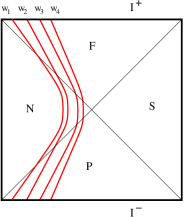
Figure 3: Two disjoint subregions $A\equiv(w_{1},w_{2})$ and
$B\equiv(w_{3},w_{4})$ at $I^{+}$ alongwith the equivalent ones at $I^{-}$,
and the corresponding future-past extremal surfaces.

This structure of these top-bottom symmetric extremal surfaces and their areas is special. Consider two disjoint subregions (restricting to top-bottom symmetric ones), defined by the boundary conditions at $I^{+}$,

$${\cal A}\equiv(w_{1},w_{2})\ ,\qquad{\cal B}\equiv(w_{3},w_{4})\ .$$ (35)

This is shown in Figure 3. One can then ask if there is any analog of the connected surfaces that arise in holographic mutual information defined as

$$I[{\cal A},{\cal B}]=S[{\cal A}]+S[{\cal B}]-S[{\cal A}\cup{\cal B}]\ .$$ (36)

In e.g. $AdS$, if the subregions ${\cal A},{\cal B}$ are far apart, then the minimal area surface for ${\cal A}\cup{\cal B}$ is simply the two disconnected surfaces around ${\cal A}$ and ${\cal B}$ so $I[{\cal A},{\cal B}]$ vanishes. However when $A,B$ are nearby, there is a new connected surface with lower area [38]: with $A\equiv(x_{1},x_{2})$ and $B\equiv(x_{3},x_{4})$, this new surface has one part with endpoints $(x_{1},x_{4})$ and another stretching between $(x_{2},x_{3})$. Since $S[{\cal A}\cup{\cal B}]$ has lower area, we have $I[{\cal A},{\cal B}]>0$. As the subsystem separation increases, the area of this new connected surface increases: at some critical separation, $S[{\cal A}\cup{\cal B}]$ equals that of the two disconnected surfaces and then $I[{\cal A},{\cal B}]$ vanishes. This is a large $N$ disentangling transition for mutual information.

In the present $dS$ case however, it appears that such new surfaces connecting the subregions ${\cal A},{\cal B}$ above cannot exist. If they did, there would be a portion of the surface that stretches between $w_{2}$ and $w_{3}$ connecting the adjacent edges of ${\cal A},{\cal B}$. However this requires a turning point for this portion of the surface which starts at $w_{2}\in I^{+}$ and returns to $w_{3}\in I^{+}$: as we have seen, such turning points do not exist, except the ones we have discussed (lying in the $N/S$ regions, which give the future-past surfaces). In other words, the only surfaces for a subregion $(w_{2},w_{3})$ comprises the future-past surfaces at $w_{2}$ and $w_{3}$, disconnected from each other: the left and right components of this are already contained in the surfaces for ${\cal A},{\cal B}$ separately. Thus it appears that mutual information vanishes always. Equivalently, for each of the boundary points $w_{I}$, there is a unique future-past surface, so the area is

$$S[{\cal A}\cup{\cal B}]=S[w_{1}]+S[w_{2}]+S[w_{3}]+S[w_{4}]=S[{\cal A}]+S[{\cal B}]\ ,$$ (37)

and $I[{\cal A},{\cal B}]$ vanishes. The ${\cal A}\cup{\cal B}$ surface is identical to the two disconnected surfaces for ${\cal A}$ and ${\cal B}$ separately. This is true for any disjoint subregions: there is no critical separation betweeen the subregions, unlike the $AdS$ case.

Now consider three adjacent regions ${\cal A},{\cal B},{\cal C}$, that do not overlap: in Figure 3, the subregions at $I^{+}$ are

$${\cal A}\equiv(w_{1},w_{2})\ ,\quad{\cal B}\equiv(w_{2},w_{3})\ ,\quad{\cal C}\equiv(w_{3},w_{4})\ ,$$ (38)

so

$${\cal A}\cup{\cal B}\equiv(w_{1},w_{3})\ ,\quad{\cal B}\cup{\cal C}\equiv(w_{2},w_{4})\ ,\quad{\cal A}\cup{\cal B}\cup{\cal C}\equiv(w_{1},w_{4})\ .$$ (39)

Then using (2.3), the areas give

$$S[{\cal A}\cup{\cal B}]+S[{\cal B}\cup{\cal C}]=S[w_{1}]+S[w_{3}]+S[w_{2}]+S[w_{4}]=S[{\cal A}\cup{\cal B}\cup{\cal C}]+S[{\cal B}]\ .$$ (40)

Thus strong subadditivity is always saturated, dovetailing in a sense with vanishing mutual information (and suggesting that tripartite information [39] as well as the entanglement wedge cross-section [40] also vanish). This fact is independent of the detailed scaling of the area with the subregion size: it follows from the fact that there is a unique surface stretching from a given boundary location $w_{0}\in I^{+}$ and that these are future-past surfaces stretching from $I^{+}\rightarrow I^{-}$, with no $I^{+}\rightarrow I^{+}$ turning point. The top-bottom symmetry that we have been focussing on has been a crucial ingredient here.

The above observations might suggest that the surfaces encode nothing, with no correlations between any two subregions at $I^{+}$. However the vanishing of mutual information here is in fact reminiscent of a finite temperature system: for subsystem sizes and separation above the scale set by the temperature, the entanglement entropy scales linearly ensuring that mutual information vanishes (see e.g. [41] for a study of holographic mutual information in finite temperature $AdS/CFT$). This appears consistent with the fact that the bulk de Sitter space is a thermodynamic object, with an entropy and a temperature (in a sense like the $AdS$ black hole): however it is perhaps a special feature that this vanishing of mutual information holds for any disjoint subregions, independent of the separation (in some sense, subregions here are already “well-separated” unlike the $AdS$ case). This is in the leading gravity (large $N$) approximation, with possibly nonvanishing subleading ($O(1)$) contributions.

3 “Entanglement wedge”: future-past surfaces

We would like to discuss the analogs of the entanglement wedge in $AdS/CFT$ [31, 32, 33] (see also the reviews e.g. [25, 26, 27]) in the present de Sitter case. Although the present case has very different features, there are analogs here of the “entanglement wedge” and subregion duality.

3.1 A codim-1 “envelope” surface from codim-2 surfaces

Given some boundary Euclidean time slice and a boundary subregion on it, we can use de Sitter isometries to generate other equivalent (codim-1) boundary subregions, since no such slice is special: e.g. a subregion with width $\Delta w$ on any $S^{d-1}$ equatorial plane can, by an asymptotic rotation, be transformed to another subregion on any $S^{d-1}$ equatorial plane. This suggests that the true bulk subregion is a codim-0 subregion with any slice giving a codim-1 subregion. Likewise in the bulk, the codim-2 extremal surface anchored at the boundary of any codim-1 subregion can be rotated to any equivalent extremal surface anchored on an equivalent subregion: this suggests that the natural bulk object is a codim-1 extremal surface obtained as a “union” or “envelope” of the family of codim-2 extremal surfaces. Although the only role of the codim-1 envelope surface is to encode the codim-2 surfaces in its slices, it is the natural object here since no boundary Euclidean time direction is sacrosanct. This codim-1 surface will play essential roles in what follows.

Note that this is not equivalent to defining the boundary subregion as the codim-0 boundary subregion $\Delta w\times S^{d-1}$ directly and constructing the corresponding codim-1 bulk extremal surface. Such a codim-1 extremal surface in $dS_{d+1}$ is described by the area functional  $S=l^{d}V_{S^{d-1}}\int{d\tau\over\tau^{d}}\ \sqrt{{1\over 1-\tau^{2}}-(1-\tau^{2})(w^{\prime})^{2}}$ and can be seen to scale as $l^{d}$. These are structurally similar to codim-2 surfaces in $dS_{d+2}$, the extremization giving

$${\dot{w}}^{2}\equiv(1-\tau^{2})^{2}\Big{(}{dw\over d\tau}\Big{)}^{2}={B^{2}\tau^{2d}\over 1-\tau^{2}+B^{2}\tau^{2d}}\ ,\qquad S={2l^{d}V_{S^{d-1}}\over 4G_{d+1}}\int_{\epsilon}^{\tau_{*}}{d\tau\over\tau^{d}}\ {1\over\sqrt{1-\tau^{2}+B^{2}\tau^{2d}}}\ ,$$ (41)

with the turning point

$$|{\dot{w}}|\rightarrow\infty:\qquad\ 1-\tau_{*}^{2}+B^{2}\tau_{*}^{2d}\ =\ 0\ .$$ (42)

These surfaces in $dS_{4}$ have a leading area divergence $S\sim 2l^{3}V_{S^{2}}\int_{\epsilon}^{1}{d\tau\over\tau^{3}}{1\over\sqrt{1-\tau^{2}}}=4\pi l^{3}({1\over\epsilon^{2}}+\log{2\over\epsilon})$, thus containing a subleading logarithmic divergence. So these ab initio codim-1 surfaces are qualitatively different from the codim-1 “envelope” surfaces described above. The latter have area scaling as de Sitter entropy on each boundary Euclidean slice with no subleading logarithmic divergence. We have constructed the codim-2 surfaces on boundary Euclidean time slices: this crutch appears in accordance with setting up a subsystem in the dual field theory on some constant Euclidean time slice and defining entanglement thereof. The effective codim-1 envelope surface arises as above since no such slice is special.

3.2 Domains of dependence and Cauchy horizons

Domains of dependence:  As we have been saying, the boundary theory is Euclidean, as are the subregions: so there is no intrinsic boundary time. Boundary Euclidean time directions, used in the construction of the extremal surfaces above, are all equivalent: these serve as a crutch to organize the surfaces simulating entanglement in the dual field theory, but they are simply spatial directions in the end.

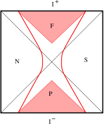
Figure 4: Generic subregion, extremal surface and domain of dependence.

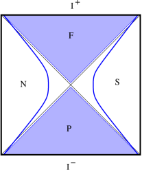
Figure 5: Subregion becoming all $I^{+}$, limiting surface, domain of dependence.

Thus, we take the only natural notion of the domain of dependence to be that defined from the bulk point of view. The natural subregion in the Euclidean boundary at $I^{+}$ is codim-0, i.e. a 3-dim subspace of the 3-dim boundary (focussing on $dS_{4}$). In order that entanglement be defined on boundary Euclidean time slices of the full space, we construct this codim-0 subregion ${\cal A}\in I^{+}$ as the interior of the boundary at $I^{+}$ of the codim-1 bulk envelope surface we have discussed above. In other words, the codim-0 boundary subregion is the interior of the codim-1 boundary obtained as the “envelope” of all the codim-2 boundaries of the codim-2 subregions. Thus this codim-0 subregion is essentially the union or envelope of the various codim-1 subregions (on boundary Euclidean time slices): the latter are of the form $\Delta w\times S^{1}$ on some equatorial plane of the $S^{2}$ in $dS_{4}$. Thus the codim-0 envelope arising as the union of the subregions on all such equatorial planes becomes $\Delta w\times S^{2}$. This is represented schematically in Figure 5 for a subregion symmetrically placed in $I^{+}$ for convenience for now (we will discuss more general subregions later). Note that these Figures are to be regarded as describing the envelope surfaces and the envelope subregions on some slice (all of which are equivalent).

Given ${\cal A}\in I^{+}$, its complement ${\cal A}_{c}$ is the rest of the boundary. Then the bulk domain of dependence of ${\cal A}$ is the past lightcone wedge of $A$, shown by the pink region in $F$ in Fig. 5. Technically, the domain of dependence of ${\cal A}$ is the set of all points $p$ such that any non-spacelike curve originating at $p$ will necessarily intersect ${\cal A}$ (see e.g. [42]). In other words, any event occurring at $p$ will necessarily influence the Cauchy data on ${\cal A}$: it is clear that this is the past lightcone of ${\cal A}$. Figure 5 shows the subregion, the corresponding extremal surface and the domain of dependence in the limit where the subregion becomes the full space.

Finally, we note again that we are restricting to top-bottom symmetric surfaces: thus the subregion ${\cal A}\in I^{+}$ has an equivalent subregion ${\bar{\cal A}}\in I^{-}$ (with a future domain of dependence, its future lightcone wedge).

Cauchy horizons: The boundary of the domain of dependence $D[{\cal A}]$ is referred to as a Cauchy horizon (see e.g. [42]). This is a boundary for the past Cauchy development of ${\cal A}\in I^{+}$ (or the future Cauchy development of ${\bar{\cal A}}\in I^{-}$). From the Cauchy data on ${\cal A}$, it is not possible to infer events outside $D[{\cal A}]$: in other words, a point outside $D[{\cal A}]$ could communicate (by sending particles/light via timelike/null trajectories) to the region outside ${\cal A}$ without influencing ${\cal A}$. Thus the boundary of $D[{\cal A}]$ is a horizon for past development of the Cauchy data on ${\cal A}$.

For the subregion ${\cal A}$ becoming the whole space, i.e. ${\cal A}\rightarrow I^{+}$, the past domain of dependence becomes the entire future universe $F$. The corresponding Cauchy horizons are then the horizons bounding $F$: these appear as event horizons to observers in the static patches which are the Northern/Southern diamonds $N/S$, but have very different nature for subregions at $I^{\pm}$.

Subregions and “causal shadows”:  We take the “causal shadow” of the subregion ${\cal A}$ to be the region outside the domain of dependence of ${\cal A}$. We see that this is the region outside the past lightcone wedge of ${\cal A}$. It is to be noted that an observer in this causal shadow region can still communicate with the subregion ${\cal A}$ (via timelike/null trajectories) so this is not quite like the $AdS$ case where the causal shadow means no communication exists: however they do not necessarily influence ${\cal A}$, lying beyond the Cauchy horizons of ${\cal A}$.

For the boundary subregion taken as ${\cal A}\cup{\cal B}$, the causal shadow is the region outside $D[{\cal A}]\cup D[{\cal B}]$, the union of the two domains of dependence. The fact that we have decomposed the boundary subregion into two disjoint subregions implies that the bulk domains of dependence $D[{\cal A}]\cup D[{\cal B}]$ are distinct from, and smaller than, $D[A\cup B]$.

For the subregion becoming the whole space, i.e. ${\cal A}\rightarrow I^{+}$, the domain of dependence is the entire future universe $F$ and the causal shadow comprises the entire Northern/Southern diamonds $N\cup S$. Similar statements hold for subregions at $I^{-}$ and the past universe $P$.

3.3 Future-past surfaces, “entanglement wedge” and subregions

Extremal surfaces and causal shadows:  We continue to focus on top-bottom symmetric subregions and the corresponding extremal surfaces. So consider a subregion ${\cal A}$ at the future boundary $I^{+}$ and its equivalent subregion at $I^{-}$ and the area of the corresponding bulk future-past extremal surface stretching between the two copies of ${\cal A}$ (e.g. the red curve in Figure 1). We would like to interpret the area of this surface as some sort of entanglement. Since this procedure requires two copies of the boundary theory, the entanglement represented by the area of the extremal surface in question is unlikely to be a boundary quantity, but is likely a bulk one. This is analogous to the fact that bulk expectation values are obtained by weighting by the bulk probability $|\Psi_{dS}|^{2}$, along the lines of $dS/CFT$ (1). The surfaces can be described as discussed earlier.

Now we note that these future-past extremal surfaces stretching between $I^{\pm}$ in fact lie in the “causal shadow”, as defined above, of the boundary subregion ${\cal A}$, as we see in Figure 5. Firstly note that we are considering the codim-1 envelope surface obtained from all the codim-2 surfaces, as we have discussed previously. The extremal surface is anchored at the boundary of the subregion ${\cal A}$ and is timelike: thus it lies outside the past lightcone wedge of ${\cal A}$ and so is in the causal shadow. It appears that this will be true for any Euclidean subregion ${\cal A}$ if the extremal surface is timelike, dipping into the holographic direction which is time in this case. This would not have been true if the extremal surface, anchored at $\partial{\cal A}$, were spacelike. Thus in fact the absence of a turning point where the surface from $I^{+}$ begins to return to $I^{+}$ ensures that the surface is timelike, thereby lying in the causal shadow of the subregion at $I^{+}$ (which is spacelike).

This appears consistent in fact with bulk causality if we take the area of these future-past extremal surfaces to encode entanglement pertaining to ${\cal A}$ (independent of the precise nature of the entanglement). Following the arguments in [33], consider any other spacelike surface ${\cal A}^{\prime}$, say with wiggles etc, but with the same boundary $\partial{\cal A}^{\prime}=\partial{\cal A}$: thus ${\cal A}^{\prime}$ is any other subregion homologously equivalent to ${\cal A}$. Then ${\cal A}^{\prime}$ has the same past domain of dependence as the original subregion ${\cal A}$ and so is expected to be unitarily equivalent to ${\cal A}$ with regard to entanglement properties: the two reduced density matrices will likely be related by the unitary transformation corresponding to bulk time evolution. Thus we expect ${\cal A}^{\prime}$ to have the same entanglement properties as ${\cal A}$, and therefore the same extremal surfaces. So we expect that the extremal surfaces should lie in the causal shadow since if they did not, they would contradict the above causality requirement.

Extremal surfaces and the “entanglement wedge”:  There have been various interesting investigations on the entanglement wedge [31, 32, 33] pertaining to extremal surfaces in $AdS/CFT$. We will now try to adapt some of those ideas and constructs to the present de Sitter case: although the spacetime structure here is quite different, we will see that some key features have analogs in this case as well.

We define the “entanglement wedge” here on a constant boundary Euclidean time slice (e.g. an $S^{d-1}$ equatorial plane) as the region enclosed between the extremal surface and the boundary subregion ${\cal A}$ on $I^{\pm}$: this gives the shaded regions in Fig. 6. The figure on the left is the entanglement wedge for the red curve in Fig. 1 while that on the right shows the limit as the subregion is becoming the whole space. In the strict limit where the subregion at $I^{\pm}$ is the whole space, the extremal surface (which is the limiting surface, sec. 2.2) is essentially contained entirely in the Northern/Southern diamond regions $N/S$. We see that the entanglement wedge now encompasses the future and past universes $F/P$, but is substantially bigger: it now contains the Cauchy horizons at $\tau=1$ entirely and a substantial portion of the $N/S$ regions. Thus while the “causal wedge”, which can be taken as the past domain of dependence in this de Sitter case, is necessarily bounded by the Cauchy horizons, the “entanglement wedge” contains more. This is reminiscent of the fact that in $AdS$, the causal wedge cannot contain points behind event horizons while the entanglement wedge can.

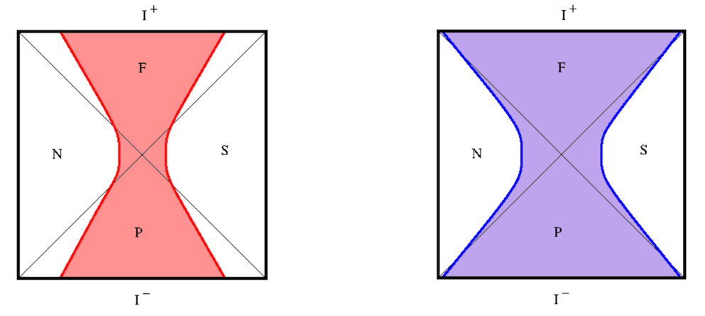
Figure 6: The “entanglement wedge” for generic extremal surface (left), the limiting surface (right).

Since the boundary dual theory is Euclidean here, no boundary Euclidean time slice can be regarded as sacrosanct as we have been discussing. Then the natural subregion is the effective codim-0 subregion on $I^{\pm}$ while the bulk region is the interior of the envelope surface obtained from the union of the codim-2 extremal surfaces. Thus the true bulk entanglement wedge should be taken as the union of the entanglement wedge on each of the slices. This generates a codim-0 bulk region corresponding to the interior of the codim-1 “envelope” surfaces obtained from the union of the codim-2 surfaces. This is represented schematically in Figure 6 (see also Figure 7).

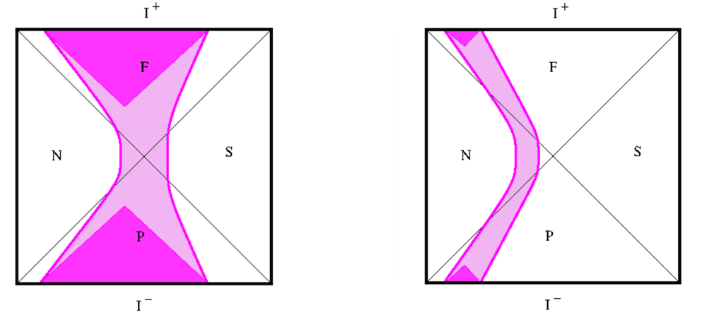
Figure 7: Some more general subregions (see e.g. Figure 2), the corresponding extremal surfaces and the associated “entanglement wedges”. Also shown within is the bulk domain of dependence of these subregions.

Subregion duality and “entanglement shadows”:  The “entanglement wedge” above appears to naturally lead to an analog of subregion duality in the de Sitter case.

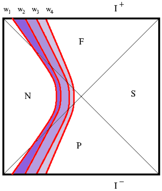
Figure 8: Multiple subregions at $I^{\pm}$ and their corresponding
top-bottom symmetric future-past extremal surfaces.
The corresponding “entanglement wedges” suggest an analog
of subregion duality.

Given a subregion at $I^{+}$ and its equivalent subregion at $I^{-}$, we have seen that the top-bottom symmetric future-past surfaces define an “entanglement wedge” which is the interior of the codim-1 envelope surface obtained from all the codim-2 extremal surfaces on boundary Euclidean time slices. For multiple disjoint subregions, the “entanglement wedges” thus obtained do not intersect or overlap: the entanglement wedges foliate the bulk space (see below however). Thus each boundary subregion at $I^{+}$ (and its equivalent one at $I^{-}$) lead to a corresponding bulk subregion defined by the “entanglement wedge” of the associated future-past extremal surface. Figure 8 shows multiple disjoint boundary subregions, the corresponding top-bottom symmetric future-past extremal surfaces and the associated “entanglement wedges”. In some sense, this appears to be the analog of subregion duality in this de Sitter case as defined by the future-past extremal surfaces we have been discussing.

It appears that a large part of the bulk space, including the future and past universes $F,P$, as well as a large part of the Northern/Southern diamond regions $N,S$, is obtainable in this manner as some bulk subregion dual to some boundary subregion. However as we have seen in sec. 2.2, in $dS_{4}$ (and higher dimensions), there is a limiting bulk extremal surface obtained as the boundary subregion becomes all $I^{\pm}$ : this surface and the corresponding “entanglement wedge” is shown in the right part of Figure 6. As is clear, the white (unshaded) regions of the Northern/Southern diamonds $N/S$, are not accessible by any of these future-past extremal surfaces. These regions appear to be “entanglement shadows”. It would be interesting to understand how precisely these parts of $N/S$ become such shadow regions.

4 Discussion

We have discussed various aspects of the future-past extremal surfaces in de Sitter space, building on previous work [29]. These are rotated analogs of the Hartman-Maldacena surfaces in the eternal $AdS$ black hole [30]. These top-bottom symmetric codim-2 surfaces (on boundary Euclidean time slices) stretch between a subregion at $I^{+}$ in the future universe $F$ and an equivalent one at $I^{-}$ in the past universe $P$, with a turning point in the Northern/Southern diamond regions $N/S$. There exists a real-valued turning point only for a certain range in $dS_{4}$ and higher dimensions: so these surfaces do not penetrate beyond a certain point in $N/S$, a limiting surface arising as the subregion at $I^{\pm}$ becomes the whole space (this limit was identified erroneously in [29]). The subregion size $\Delta w$ for this limiting surface acquires a logarithmic divergence, as we saw in Sec. 2.2.

For a given subregion at $I^{\pm}$ as in Figure 1 or Figure 2, the full top-bottom symmetric surface consists of the left and right portions: each of these connects $I^{\pm}$ but is disconnected from the other portion. This disconnectedness reflects the fact that a surfaces anchored at $I^{+}$ does not return to $I^{+}$ but ends at $I^{-}$. This then implies that for multiple disjoint subregions, mutual information vanishes, as we discussed in Sec. 2.3. This is reminiscent of a finite temperature system in $AdS/CFT$, perhaps reflecting the fact that the bulk de Sitter space has a temperature (in some sense, de Sitter space being thermodynamic is akin to the $AdS$ black hole, rather than pure $AdS$). This disconnectedness further implies that strong subadditivity is saturated. Also, it suggests related points, such as vanishing tripartite information [39] and vanishing entanglement wedge cross-section [40]. It is important to note that the analysis here is all in the leading gravity (large $N$) approximation: presumably subleading contributions (at $O(1)$ order) will lead to non-vanishing entanglement quantities. It would be interesting to explore further properties/inequalities that these surfaces satisfy, and their implications via $dS/CFT$. In this regard, since the dual CFT is expected to be non-unitary, it must be noted that the interpretations thereof (e.g. vanishing leading mutual information suggesting no correlations) may be different from those in ordinary unitary theories.

Since the Euclidean boundary theory has no intrinsic time (all boundary slices are equivalent), these codim-2 surfaces define an effective codim-1 “envelope” surface and (in $dS_{d+1}$) a codim-0 boundary subregion $\Delta w\times S^{d-1}$, as we saw in Sec. 3.1. This leads to analogs of the entanglement wedge for these future-past extremal surfaces as we saw in Sec. 3. The associated “entanglement wedge” defined as the bulk region bounded by the extremal surfaces and the boundary subregions is a bigger region than the “causal wedge” (or the domain of dependence) for the subregion in question. This “entanglement wedge” suggests an analog of subregion duality, Figure 8: the bulk subregion enclosed by the extremal surfaces and the boundary subregions at $I^{\pm}$ is dual to the boundary subregion in question. For the limiting surface, corresponding to the boundary subregion becoming all of $I^{+}$, the “entanglement wedge” covers the future-past universes $F/P$ as well as a substantial part of the Northern/Southern diamond regions $N/S$. However there is a substantial “shadow” part of $N/S$ which is not accessible via these extremal surfaces for $dS_{4}$ and higher dimensions (it is interesting to ask if these regions of $N/S$ can be described by e.g. analogs of mirror operators [43]).

Our analysis here has been based on the geometric properties of these future-past extremal surfaces, and therefore heuristic in some essential sense. It would be interesting to understand more directly if these heuristic geometric observations can be made more precise towards better understanding the physical interpretation, for instance via the analog in $dS/CFT$ of the interrelations between the entanglement wedge, modular flow, relative entropy, error correction codes and so on [44, 45, 46] (see also the reviews [25, 26, 27]). It would also be interesting to understand the role of HKLL bulk reconstruction [47, 48, 49] with regard to these future-past extremal surfaces (see e.g. [21] in the higher spin $dS/CFT$ context; see also [50, 51]).

Our discussions so far have focussed on bulk extremal surfaces. Operationally we have considered a boundary (spatial) subregion at $I^{+}$ and its equivalent boundary subregion at $I^{-}$, and extremal surfaces stretching between them through the holographic (time) direction. The top-bottom symmetry in some sense simulates the bulk inner product $\Psi_{I^{+}}^{*}{\cal O}\Psi_{I^{+}}$, with $\Psi_{I^{-}}\equiv\Psi_{I^{+}}^{*}$ (it is in some sense reminiscent of the in-in formalism). By focussing first on boundary Euclidean time slices, we have simulated setting up entanglement entropy in the dual field theory, leading to codim-2 surfaces: the fact that these slices are all equivalent leads to an effective codim-1 envelope surface. The area of these future-past codim-2 surfaces is positive and exhibits (for $dS_{4}$) an area law divergence ${l^{2}\over G_{4}}{1\over\epsilon}$ for generic subregions: the finite part scales as ${l^{2}\over G_{4}}\Delta w$ linearly with the subregion size $\Delta w$ as the subregions become all $I^{\pm}$. The coefficients scale as $dS_{4}$ entropy, which is akin to the number of degrees of freedom in the dual $CFT$. The fact that these future-past surfaces are defined with two boundaries suggests that the area is a sort of bulk entanglement entropy, especially if we take the (analog of) subregion duality above seriously. Thus overall these future-past extremal surfaces are perhaps best interpreted as a way to organize bulk entanglement in terms of boundary subregions in de Sitter space (in some sense, these surfaces suggest entanglement between timelike separated regions; see below). It would be interesting to clarify this further. Relatedly, it would also be useful to explore more general boundary subregions (e.g. caps on the sphere $S^{d-1}$ etc): in such cases we feel similar future-past extremal surfaces will arise but these appear difficult to analyse in detail, so it is unclear if the various features we have noted here will hold more generally (including for subregions that are not top-bottom symmetric, as might arise under e.g. a shock wave perturbation in the bulk).

From the dual point of view, ghost-like CFTs as [10], [12], might suggest, are expected to have negative norm states/configurations, thus suggesting “negative entanglement”. Various investigations involving ghost-like theories, including simple toy quantum-mechanical models of “ghost-spins”, in fact exhibit this non-positive entanglement quite explicitly, e.g. [52, 53] (reviewed in [28]). However, “correlated” states entangling identical ghost-spins between two copies of ghost-spin ensembles can be shown to have positive norm, reduced density matrices (RDMs) and entanglement. Considering two copies of 3-dim $N$-level ghost-spin systems as microscopic realizations in the universality class of ghost-$CFT_{3}$’s dual to $dS_{4}$ with $N\sim{l^{2}\over G_{4}}$ finite albeit large, “correlated” states [29] of the form $|\psi\rangle=\sum\psi^{i_{n}^{F},i_{n}^{P}}|i_{n}\rangle_{{}_{F}}|i_{n}\rangle_{{}_{P}}$ entangling ghost-spin configurations $|i_{n}\rangle_{{}_{F}}$ from $CFT_{F}$ at $I^{+}$ with identical ones $|i_{n}\rangle_{{}_{P}}$ from $CFT_{P}$ at $I^{-}$, are entirely positive, giving positive RDM and entanglement. These are in some sense consistent with the top-bottom symmetric future-past surfaces we have been discussing, stretching between $I^{\pm}$. Bulk time evolution maps states at $I^{-}$ to $I^{+}$ [9], and suggests the states above are unitarily equivalent to entangled states in two $CFT_{F}$ copies solely at $I^{+}$. $CFT_{P}\equiv CFT_{F}$ implies a single $CFT$, but the state above is perhaps best regarded as a particular entangled slice in a doubled system, akin to the thermofield double dual to the eternal $AdS$ black hole [54]. This suggests the speculation [29] that $dS_{4}$ is perhaps approximately dual to $CFT_{F}\times CFT_{P}$ (or $CFT_{F}\times CFT_{F}$) entangled as above, $dS_{4}$ entropy arising as entanglement. See also [55] for a related discussion.

It would appear that our discussions here are consistent with the natural holographic screens for de Sitter space (obtained via mapping along light rays) being at future and past timelike infinity [56] (see [11] for an early discussion of holography and asymptotics, and elaborated on for de Sitter space [8, 9]). Both boundaries $I^{\pm}$ are required: these are thus preferred screens for anchoring the future-past extremal surfaces. Since these surfaces intersect all $\tau=const$ surfaces in $F/P$ precisely once, it would appear that moving the screens towards the interior (i.e. moving the screens from $I^{\pm}$ at $\tau=\epsilon\sim 0$ to say $\tau=\tau_{0}$ with $\epsilon<\tau_{0}\ll 1$) does not affect the construction of these extremal surfaces. How this gels with e.g. the area law in [57] will be interesting to understand. It would also be interesting to understand other screens such as the Poincare horizon [56]: see e.g. [58]. One might hope that the considerations here may help in understanding and organizing holography for cosmologies more generally.

Finally, all our explorations here have been analogs of the classical RT/HRT story in $AdS/CFT$, viewed via a $dS/CFT$ perspective (see [59, 60] for a different approach, based on the dS/dS correspondence [61]): it would be interesting to understand if these investigations can be obtained via analogs of [62] or bulk replicas [63, 64]. It would then be interesting to understand subleading corrections, quantum extremal surfaces [65, 66] and beyond.

Acknowledgements:  It is a pleasure to thank Dionysios Anninos, Rajesh Gopakumar, Tom Hartman, Matt Headrick, Kedar Kolekar, Alok Laddha, R. Loganayagam and especially Suvrat Raju for helpful discussions and comments on a draft. I’ve also benefitted from early discussions with Dionysios Anninos, Juan Maldacena, Kyriakos Papadodimas and Shahin Sheikh-Jabbari on previous work. This work is partially supported by a grant to CMI from the Infosys Foundation.

References

- [1]
- [2] G. W. Gibbons and S. W. Hawking, “Cosmological Event Horizons, Thermodynamics, and Particle Creation,” Phys. Rev. D 15, 2738 (1977). doi:10.1103/PhysRevD.15.2738
- [3] M. Spradlin, A. Strominger and A. Volovich, “Les Houches lectures on de Sitter space,” hep-th/0110007.
- [4] J. M. Maldacena, “The large N limit of superconformal field theories and supergravity,” Adv. Theor. Math. Phys. 2, 231 (1998) [Int. J. Theor. Phys. 38, 1113 (1999)] [arXiv:hep-th/9711200].
- [5] S. S. Gubser, I. R. Klebanov and A. M. Polyakov, “Gauge theory correlators from non-critical string theory,” Phys. Lett. B 428, 105 (1998) [arXiv:hep-th/9802109].
- [6] E. Witten, “Anti-de Sitter space and holography,” Adv. Theor. Math. Phys. 2, 253 (1998) [arXiv:hep-th/9802150].
- [7] O. Aharony, S. S. Gubser, J. M. Maldacena, H. Ooguri and Y. Oz, “Large N field theories, string theory and gravity,” Phys. Rept. 323, 183 (2000) [arXiv:hep-th/9905111].
- [8] A. Strominger, “The dS / CFT correspondence,” JHEP 0110, 034 (2001) [hep-th/0106113].
- [9] E. Witten, “Quantum gravity in de Sitter space,” [hep-th/0106109].
- [10] J. M. Maldacena, “Non-Gaussian features of primordial fluctuations in single field inflationary models,” JHEP 0305, 013 (2003), [astro-ph/0210603].
-
[11]
E. Witten, Talk at Strings 98 conference, Santa Barbara, USA, 1998,
http://online.itp.ucsb.edu/online/strings98/witten/. - [12] D. Anninos, T. Hartman and A. Strominger, “Higher Spin Realization of the dS/CFT Correspondence,” Class. Quant. Grav. 34, no. 1, 015009 (2017) doi:10.1088/1361-6382/34/1/015009 [arXiv:1108.5735 [hep-th]].
- [13] R. Bousso, A. Maloney and A. Strominger, “Conformal vacua and entropy in de Sitter space,” Phys. Rev. D 65, 104039 (2002) [hep-th/0112218].
- [14] V. Balasubramanian, J. de Boer and D. Minic, “Notes on de Sitter space and holography,” Class. Quant. Grav. 19, 5655 (2002) [Annals Phys. 303, 59 (2003)] [hep-th/0207245].
- [15] D. Harlow and D. Stanford, “Operator Dictionaries and Wave Functions in AdS/CFT and dS/CFT,” arXiv:1104.2621 [hep-th].
- [16] G. S. Ng and A. Strominger, “State/Operator Correspondence in Higher-Spin dS/CFT,” Class. Quant. Grav. 30, 104002 (2013) [arXiv:1204.1057 [hep-th]].
- [17] D. Anninos, “De Sitter Musings,” Int. J. Mod. Phys. A 27, 1230013 (2012) [arXiv:1205.3855 [hep-th]].
- [18] D. Das, S. R. Das, A. Jevicki and Q. Ye, “Bi-local Construction of Sp(2N)/dS Higher Spin Correspondence,” JHEP 1301, 107 (2013) [arXiv:1205.5776 [hep-th]].
- [19] D. Anninos, F. Denef and D. Harlow, “The Wave Function of Vasiliev’s Universe - A Few Slices Thereof,” Phys. Rev. D 88, 084049 (2013) [arXiv:1207.5517 [hep-th]].
- [20] S. Banerjee, A. Belin, S. Hellerman, A. Lepage-Jutier, A. Maloney, D. Radicevic and S. Shenker, “Topology of Future Infinity in dS/CFT,” JHEP 1311, 026 (2013) [arXiv:1306.6629 [hep-th]].
- [21] D. Anninos, F. Denef, R. Monten and Z. Sun, “Higher Spin de Sitter Hilbert Space,” JHEP 1910, 071 (2019) doi:10.1007/JHEP10(2019)071 [arXiv:1711.10037 [hep-th]].
- [22] S. Ryu and T. Takayanagi, “Holographic derivation of entanglement entropy from AdS/CFT,” Phys. Rev. Lett. 96, 181602 (2006) [hep-th/0603001].
- [23] S. Ryu and T. Takayanagi, “Aspects of Holographic Entanglement Entropy,” JHEP 0608, 045 (2006) [hep-th/0605073].
- [24] V. E. Hubeny, M. Rangamani and T. Takayanagi, “A Covariant holographic entanglement entropy proposal,” JHEP 0707 (2007) 062 [arXiv:0705.0016 [hep-th]].
- [25] M. Rangamani and T. Takayanagi, “Holographic Entanglement Entropy,” Lect. Notes Phys. 931, pp.1 (2017) [arXiv:1609.01287 [hep-th]].
- [26] D. Harlow, “TASI Lectures on the Emergence of Bulk Physics in AdS/CFT,” PoS TASI 2017, 002 (2018) doi:10.22323/1.305.0002 [arXiv:1802.01040 [hep-th]].
- [27] M. Headrick, “Lectures on entanglement entropy in field theory and holography,” arXiv:1907.08126 [hep-th].
- [28] K. Narayan, “de Sitter entropy as entanglement,” Honorable Mention, Gravity Research Foundation 2019 Awards for Essays on Gravitation, Int. J. Mod. Phys. D 28, no. 14, 1944019 (2019), doi:10.1142/S021827181944019X , [arXiv:1904.01223 [hep-th]].
- [29] K. Narayan, “On extremal surfaces and de Sitter entropy,” Phys. Lett. B 779, 214 (2018) [arXiv:1711.01107 [hep-th]].
- [30] T. Hartman and J. Maldacena, “Time Evolution of Entanglement Entropy from Black Hole Interiors,” JHEP 1305, 014 (2013) [arXiv:1303.1080 [hep-th]].
- [31] B. Czech, J. L. Karczmarek, F. Nogueira and M. Van Raamsdonk, “The Gravity Dual of a Density Matrix,” Class. Quant. Grav. 29, 155009 (2012) doi:10.1088/0264-9381/29/15/155009 [arXiv:1204.1330 [hep-th]].
- [32] A. C. Wall, “Maximin Surfaces, and the Strong Subadditivity of the Covariant Holographic Entanglement Entropy,” Class. Quant. Grav. 31, no. 22, 225007 (2014) doi:10.1088/0264-9381/31/22/225007 [arXiv:1211.3494 [hep-th]].
- [33] M. Headrick, V. E. Hubeny, A. Lawrence and M. Rangamani, “Causality & holographic entanglement entropy,” JHEP 1412, 162 (2014) doi:10.1007/JHEP12(2014)162 [arXiv:1408.6300 [hep-th]].
- [34] K. Narayan, “de Sitter extremal surfaces,” Phys. Rev. D 91, no. 12, 126011 (2015) [arXiv:1501.03019 [hep-th]].
- [35] K. Narayan, “de Sitter space and extremal surfaces for spheres,” Phys. Lett. B 753, 308 (2016) [arXiv:1504.07430 [hep-th]].
- [36] Y. Sato, “Comments on Entanglement Entropy in the dS/CFT Correspondence,” Phys. Rev. D 91, no. 8, 086009 (2015) [arXiv:1501.04903 [hep-th]].
- [37] M. Miyaji and T. Takayanagi, “Surface/State Correspondence as a Generalized Holography,” PTEP 2015, no. 7, 073B03 (2015) doi:10.1093/ptep/ptv089 [arXiv:1503.03542 [hep-th]].
- [38] M. Headrick, “Entanglement Renyi entropies in holographic theories,” Phys. Rev. D 82, 126010 (2010) doi:10.1103/PhysRevD.82.126010 [arXiv:1006.0047 [hep-th]].
- [39] P. Hayden, M. Headrick and A. Maloney, “Holographic Mutual Information is Monogamous,” Phys. Rev. D 87, no. 4, 046003 (2013) doi:10.1103/PhysRevD.87.046003 [arXiv:1107.2940 [hep-th]].
- [40] T. Takayanagi and K. Umemoto, “Entanglement of purification through holographic duality,” Nature Phys. 14, no. 6, 573 (2018) doi:10.1038/s41567-018-0075-2 [arXiv:1708.09393 [hep-th]].
- [41] W. Fischler, A. Kundu and S. Kundu, “Holographic Mutual Information at Finite Temperature,” Phys. Rev. D 87, no. 12, 126012 (2013) doi:10.1103/PhysRevD.87.126012 [arXiv:1212.4764 [hep-th]].
- [42] S. W. Hawking and G. F. R. Ellis, “The Large Scale Structure of Space-Time,” doi:10.1017/CBO9780511524646
- [43] K. Papadodimas and S. Raju, “State-Dependent Bulk-Boundary Maps and Black Hole Complementarity,” Phys. Rev. D 89, no. 8, 086010 (2014) [arXiv:1310.6335 [hep-th]].
- [44] A. Almheiri, X. Dong and D. Harlow, “Bulk Locality and Quantum Error Correction in AdS/CFT,” JHEP 1504, 163 (2015) doi:10.1007/JHEP04(2015)163 [arXiv:1411.7041 [hep-th]].
- [45] D. L. Jafferis, A. Lewkowycz, J. Maldacena and S. J. Suh, “Relative entropy equals bulk relative entropy,” JHEP 1606, 004 (2016) doi:10.1007/JHEP06(2016)004 [arXiv:1512.06431 [hep-th]].
- [46] X. Dong, D. Harlow and A. C. Wall, “Reconstruction of Bulk Operators within the Entanglement Wedge in Gauge-Gravity Duality,” Phys. Rev. Lett. 117, no. 2, 021601 (2016) doi:10.1103/PhysRevLett.117.021601 [arXiv:1601.05416 [hep-th]].
- [47] A. Hamilton, D. N. Kabat, G. Lifschytz and D. A. Lowe, “Local bulk operators in AdS/CFT: A Boundary view of horizons and locality,” Phys. Rev. D 73, 086003 (2006) doi:10.1103/PhysRevD.73.086003 [hep-th/0506118].
- [48] A. Hamilton, D. N. Kabat, G. Lifschytz and D. A. Lowe, “Holographic representation of local bulk operators,” Phys. Rev. D 74, 066009 (2006) doi:10.1103/PhysRevD.74.066009 [hep-th/0606141].
- [49] A. Hamilton, D. N. Kabat, G. Lifschytz and D. A. Lowe, “Local bulk operators in AdS/CFT: A Holographic description of the black hole interior,” Phys. Rev. D 75, 106001 (2007) Erratum: [Phys. Rev. D 75, 129902 (2007)] doi:10.1103/PhysRevD.75.106001, 10.1103/PhysRevD.75.129902 [hep-th/0612053].
- [50] X. Xiao, “Holographic representation of local operators in de sitter space,” Phys. Rev. D 90, no. 2, 024061 (2014) doi:10.1103/PhysRevD.90.024061 [arXiv:1402.7080 [hep-th]].
- [51] D. Sarkar and X. Xiao, “Holographic Representation of Higher Spin Gauge Fields,” Phys. Rev. D 91, no. 8, 086004 (2015) doi:10.1103/PhysRevD.91.086004 [arXiv:1411.4657 [hep-th]].
- [52] K. Narayan, “On extremal surfaces and entanglement entropy in some ghost CFTs,” Phys. Rev. D 94, no. 4, 046001 (2016) [arXiv:1602.06505 [hep-th]].
- [53] D. P. Jatkar and K. Narayan, “Ghost-spin chains, entanglement and -ghost CFTs,” Phys. Rev. D 96, no. 10, 106015 (2017) [arXiv:1706.06828 [hep-th]].
- [54] J. M. Maldacena, “Eternal black holes in anti-de Sitter,” JHEP 0304, 021 (2003) [hep-th/0106112].
- [55] C. Arias, F. Diaz and P. Sundell, “De Sitter Space and Entanglement,” Class. Quant. Grav. 37, no. 1, 015009 (2020) doi:10.1088/1361-6382/ab5b78 [arXiv:1901.04554 [hep-th]].
- [56] R. Bousso, “Holography in general space-times,” JHEP 9906, 028 (1999) doi:10.1088/1126-6708/1999/06/028 [hep-th/9906022].
- [57] R. Bousso and N. Engelhardt, “New Area Law in General Relativity,” Phys. Rev. Lett. 115, no. 8, 081301 (2015) doi:10.1103/PhysRevLett.115.081301 [arXiv:1504.07627 [hep-th]].
- [58] F. Sanches and S. J. Weinberg, “Holographic entanglement entropy conjecture for general spacetimes,” Phys. Rev. D 94, no. 8, 084034 (2016) doi:10.1103/PhysRevD.94.084034 [arXiv:1603.05250 [hep-th]].
- [59] A. Lewkowycz, J. Liu, E. Silverstein and G. Torroba, “ and EE, with implications for (A)dS subregion encodings,” arXiv:1909.13808 [hep-th].
- [60] H. Geng, “Some Information Theoretic Aspects of De-Sitter Holography,” JHEP 2002, 005 (2020) doi:10.1007/JHEP02(2020)005 [arXiv:1911.02644 [hep-th]].
- [61] M. Alishahiha, A. Karch, E. Silverstein and D. Tong, “The dS/dS correspondence,” AIP Conf. Proc. 743, no. 1, 393 (2004) [hep-th/0407125].
- [62] H. Casini, M. Huerta and R. C. Myers, “Towards a derivation of holographic entanglement entropy,” JHEP 1105, 036 (2011) [arXiv:1102.0440 [hep-th]].
- [63] A. Lewkowycz and J. Maldacena, “Generalized gravitational entropy,” JHEP 1308, 090 (2013) doi:10.1007/JHEP08(2013)090 [arXiv:1304.4926 [hep-th]].
- [64] X. Dong, A. Lewkowycz and M. Rangamani, “Deriving covariant holographic entanglement,” JHEP 1611, 028 (2016) doi:10.1007/JHEP11(2016)028 [arXiv:1607.07506 [hep-th]].
- [65] T. Faulkner, A. Lewkowycz and J. Maldacena, “Quantum corrections to holographic entanglement entropy,” JHEP 1311, 074 (2013) doi:10.1007/JHEP11(2013)074 [arXiv:1307.2892 [hep-th]].
- [66] N. Engelhardt and A. C. Wall, “Quantum Extremal Surfaces: Holographic Entanglement Entropy beyond the Classical Regime,” JHEP 1501, 073 (2015) doi:10.1007/JHEP01(2015)073 [arXiv:1408.3203 [hep-th]].