Finite-temperature properties of excitonic condensation in the extended Falicov-Kimball model: Cluster mean-field-theory approach

Abstract

We study the electron-hole pair (or excitonic) condensation in the extended Falicov-Kimball model at finite temperatures based on the cluster mean-field-theory approach, where we make the grand canonical exact-diagonalization analysis of small clusters using the sine-square deformation function. We thus calculate the ground-state and finite-temperature phase diagrams of the model, as well as its optical conductivity and single-particle spectra, thereby clarifying how the preformed pair states appear in the strong-coupling regime of excitonic insulators. We compare our results with experiments on Ta₂NiSe₅.

The electron-hole pair (or excitonic) condensation [1, 2, 3] in transition-metal chalcogenides and oxides has attracted much attention in recent years [4, 5]. One of the representative materials is Ta₂NiSe₅ [6, 7, 8, 9], where it was pointed out that the system is a spin-singlet excitonic insulator (EI) in the strong-coupling regime, so that the conventional phase diagram [10] breaks down [11]; i.e., even though the noninteracting band structure is semimetallic, the system above the transition temperature ($T_{c}$) is not a semimetal, but rather a state of strongly coupled preformed pairs with a finite band gap. A novel insulator state exhibiting a variety of intriguing physical properties is thus expected to occur. However, not much is known about the preformed pair states in EI models, among which the simplest spinless fermion model for spin-singlet excitonic condensation is the extended Falicov-Kimball model (EFKM) [12, 13].

In this paper, we study finite-temperature properties of the EFKM at half filling using the cluster mean-field-theory (CMFT) approach [14, 15, 16, 17, 18, 19], whereby we can take into account the quantum (as well as thermal) fluctuations of the system, allowing for any finite-temperature phase transition. We make a grand canonical exact-diagonalization analysis of small clusters, employing the so-called sine-square deformation (SSD) function [20, 21]. Thus, we calculate a number of physical quantities in the semi-thermodynamic limit, which can be approached by a small-cluster analysis.

In what follows, we will first present the model and method of our calculations; in particular, we discuss the CMFT approach using the grand canonical exact-diagonalization analysis of small clusters in some detail, where we use the SSD function. We will then show our results for the ground-state and finite-temperature phase diagrams of the model. We will also show temperature dependence of the optical conductivity and single-particle spectra, thereby clarifying how the preformed pair states appear in the strong-coupling regime of the EIs. Finally, we will compare our results with experiments on Ta₂NiSe₅ and discuss implications of our results to the strong-coupling nature of the EI states.

We thus shed some light on the finite-temperature properties, or the preformed pair states above $T_{c}$, of the strong-coupling regime of the EIs for the first time, the clarification of which has long been sought for [11] but, to the best of our knowledge, has not been fully discussed so far.

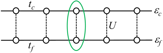
Figure 1: (Color online) Schematic representation of the 1D EFKM. The mean-field bond is indicated by an ellipse.

A minimal theoretical model for the spin-singlet EI states, such as in Ta₂NiSe₅, is the Falicov-Kimball model [22] extended by including a finite width of the valence band, which is referred to as the EFKM [12, 13]. The Hamiltonian reads

$$\cal{H} =-t_{c}\sum_{\langle i,j\rangle}c_{i}^{\dagger}c_{j}-t_{f}\sum_{\langle i,j\rangle}f_{i}^{\dagger}f_{j}+U\sum_{i}c_{i}^{\dagger}c_{i}f_{i}^{\dagger}f_{i}$$

$$+(\varepsilon_{c}-\mu)\sum_{i}c_{i}^{\dagger}c_{i}+(\varepsilon_{f}-\mu)\sum_{i}f_{i}^{\dagger}f_{i},$$ (1)

where $c_{i}$ and $f_{i}$ are annihilation operators of spinless fermions (which is referred to as an electron hereafter) in the conduction-band ($c$) and valence-band ($f$) orbitals at site $i$, respectively. We define the energy-level splitting between the $c$ and $f$ orbitals as $D=\varepsilon_{c}-\varepsilon_{f}$ $(>0)$, and the hopping parameters in the respective orbitals as $t_{c}$ and $t_{f}$. $\mu$ is the chemical potential. Regarding the modeling of Ta₂NiSe₅, we consider a one-dimensional (1D) lattice under the implicit assumption of the presence of weak three-dimensionality (see below), representing a direct band-gap semiconductor (or a semimetal) with $t_{c}$ $(>0)$ and $t_{f}$ $(<0)$, where the direct hopping of electrons between the $c$ and $f$ orbitals is prohibited (see Fig. 1). We assume the on-site Coulomb repulsion between electrons to be $U$, which acts as the on-site attractive interaction between an electron and a hole. We restrict ourselves to the case at half-filling, so that we have either a semiconductor at $D>2(t_{c}+|t_{f}|$) or a semimetal at $D<2(t_{c}+|t_{f}|$) when $U=0$. Hereafter, we assume $t_{c}=1$ (unit of energy) and $t_{f}=-0.3$, unless otherwise indicated.

Here, we note that, since the direct hopping of electrons between the $c$ and $f$ orbitals is prohibited in this model, the operators of the total number of electrons in each orbital have a simultaneous eigenstate of the Hamiltonian, so that any physical quantity changes discontinuously (due to discontinuous change in the total number of electrons in each orbital) when calculated, e.g., as a function of the parameters involved in the Hamiltonian. In small-cluster calculations, this situation leads to an apparently unphysical parameter dependence of the calculated physical quantity. However, we will show below that this difficulty may essentially be suppressed by introducing the SSD function to our exact-diagonalization calculations of small clusters.

We employ the CMFT to study phase transitions emerging in the system. In the CMFT, since only a part of the cluster (a site and/or a bond) is replaced by a mean field, quantum (as well as thermal) fluctuations within the cluster size can be taken into account [23]. The phase transition is then detected directly by a nonzero value of the mean field, which is regarded as the order parameter of the phase transition, as in the conventional mean-field theory. A recent example is the application of the CMFT to the 1D Heisenberg model for discussing the finite-temperature phase transition [19, 24], where a customary assumption is adopted that the weak three-dimensional interchain coupling is implicitly introduced via the mean-field in the CMFT calculation, just as in our present calculation.

We note here that the finite-temperature phase transition can be obtained in the conventional mean-field theory, but the effects of the fluctuations above $T_{c}$ cannot be seen. In the CMFT, however, we can obtain the finite-temperature phase transition and at the same time the effects of the fluctuations above $T_{c}$ can be observed, as we will see below. We also note that the density-matrix renormalization group (DMRG) calculation of the 1D EFKM has provided a successful results at zero temperature [25], which is however not suited for finite-temperature calculations of the present model [26].

We use finite-size clusters with $L\times 2$ orbitals, where the length $L$ is fixed to be odd. Then, the Coulomb term at the center of the system is replaced by a mean-field bond (see Fig. 1), namely,

$$c_{i}^{\dagger}c_{i}f_{i}^{\dagger}f_{i}\simeq\langle c_{i}^{\dagger}c_{i}\rangle f_{i}^{\dagger}f_{i} +\langle f_{i}^{\dagger}f_{i}\rangle c_{i}^{\dagger}c_{i}$$

$$-\langle f_{i}^{\dagger}c_{i}\rangle c_{i}^{\dagger}f_{i}-\langle c_{i}^{\dagger}f_{i}\rangle f_{i}^{\dagger}c_{i},$$ (2)

where $\langle\cdots\rangle$ denotes the expectation value with respect to the ground state of the system at temperature $T=0$, while at finite $T$, it denotes the canonical average of an operator $A$ defined as $\langle A\rangle=\mathrm{Tr}\,A\exp(-\beta\mathcal{H})/Z$, $Z=\mathrm{Tr}\exp(-\beta\mathcal{H})$, and $\beta=1/T$. Here, the Hamiltonian including the mean-field bond is solved numerically by a full exact-diagonalization of the cluster. Thus, the mean-field values $\langle c_{i}^{\dagger}c_{i}\rangle$, $\langle f_{i}^{\dagger}f_{i}\rangle$, $\langle f_{i}^{\dagger}c_{i}\rangle$, and $\langle c_{i}^{\dagger}f_{i}\rangle$ are calculated self-consistently. The chemical potential $\mu$ is also determined so as to fulfill the condition $\langle c_{i}^{\dagger}c_{i}\rangle+\langle f_{i}^{\dagger}f_{i}\rangle=1$.

Now, let us compute the mean-field values defined above. Since they are local quantities, we may approximately obtain them in the bulk limit even within the use of small clusters by applying the ‘grand canonical’ analysis. In this analysis, the original Hamiltonian consisting of local terms $\mathcal{H}_{i}$, defined as in Ref. [20], is deformed as

$${\mathcal{H}}_{\rm deform}=\sum_{i=1}^{L}{\mathcal{H}}_{i}f(\bm{r}_{i}),$$ (3)

where $f(\bm{r})$ is an externally given function, which varies smoothly from the maximum at the center of the cluster [$i=(L+1)/2$] to zero at the edges of the cluster. For such a function, we typically adopt the so-called sine-square deformation (SSD) function, which provides a smooth boundary condition. For the 1D system, the SSD function is given as

$$f_{\rm SSD}(i)=\sin^{2}\left(\frac{\pi}{L}\big{(}i-\frac{1}{2}\big{)}\right)$$ (4)

with either $i=1,\cdots,L$ for the on-site and $U$ terms or $i=3/2,\cdots,L-1/2$ for the hopping terms between sites $i$ and $i+1$. This deformation spatially scales down the energy from unity at the system center toward zero at the open edge sites, which introduces the renormalization of the energy levels in a way reminiscent of Wilson’s numerical renormalization group [21, 27]. As a consequence, the local quantities around the system center are self-organized to tune the particle number of the bulk states to their thermodynamic limit by using the edges as a reservoir. In this way, our grand canonical analysis using SSD optimally realizes the bulk eigenstate basis at the center of a small cluster. Smooth variations of the physical quantities calculated as a function of temperature, as well as of the internal parameters of the EFKM, are thereby demonstrated, as we will show below.

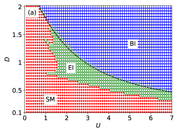
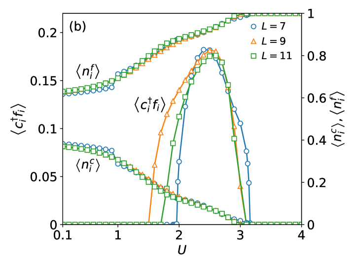
Figure 2: (Color online) (a) Calculated ground-state phase diagram of the EFKM on the $(U,D)$ plane, which contains the BI (blue), EI (green), and normal SM (red) phases. The dashed line indicates the exact analytical solution of the BI-EI phase boundary. The cluster of $L=9$ is used. (b) Calculated order parameter $\langle c_{i}^{\dagger}f_{i}\rangle$ and numbers of electrons in the $c$ and $f$ orbitals $\langle n_{i}^{c}\rangle$ and $\langle n_{i}^{f}\rangle$ as a function of $U$. $D=1$ is assumed. We compare the results obtained for the clusters of $L=7$ (blue), $L=9$ (orange), and $L=11$ (green).

First, let us discuss the ground state of the EFKM at $T=0$ K. The calculated ground-state phase diagram of the model is shown in Fig. 2(a) on the $(U,D)$ plane, where we find that the excitonic insulator (EI) phase actually occurs between the band insulator (BI) and normal semimetallic (SM) phases. The calculated phase boundary between the BI and EI phases agrees well with the exact BI-EI phase boundary $D=\sqrt{4(t_{c}+|t_{f}|)^{2}+U^{2}}-U$ obtained analytically [28] and indicated by the dashed line. Here, we do not take into account the staggered orbital order phase, which should appear around $D=0$ [25].

We note that, unlike in the numerically exact DMRG solution given in Ref. [25], the EI phase appears only near the BI-EI phase boundary. This is because the EI phase cannot acquire sufficient energy-gain in the small $U$ region in the present CMFT calculations. In this region, the energy-gain in the EI-state formation is exponentially small. We then suggest that the absence of the EI phase at small $U$ is an artifact of the SSD because some uncertainty in the electron number is always involved when applying the SSD [21], just as the Mott insulating state immediately destabilized away from half-filling at small $U$ even within the mean-field level.

We also note that the phase boundary between the EI and SM phases exhibits a nonmonotonous curve, which may be due to the above-discussed discontinuous behavior of small clusters of the EFKM. However, we should emphasize that the CMFT calculation indeed successfully provides the continuous EI phase between the BI and SM phases with the help of the SSD function.

The calculated order parameter $\langle c_{i}^{\dagger}f_{i}\rangle$ and numbers of electrons in the $c$ and $f$ orbitals $\langle n_{i}^{c}\rangle=\langle c_{i}^{\dagger}c_{i}\rangle$ and $\langle n_{i}^{f}\rangle=\langle f_{i}^{\dagger}f_{i}\rangle$ are shown in Fig. 2(b) as a function of $U$ at $D=1$ for the clusters of $L=7$, $9$, and $11$. We find that the cluster-size dependence of the results, even for the order parameter $\langle c_{i}^{\dagger}f_{i}\rangle$, is not very strong. We also find that the numbers of electrons $\langle n_{i}^{c}\rangle$ and $\langle n_{i}^{f}\rangle$ vary smoothly as a function of $U$ owing to the SSD function, although we still notice a small discontinuity at $U\simeq 1$ for the $L=7$ cluster. We find again that $\langle c_{i}^{\dagger}f_{i}\rangle$ vanishes rather rapidly when $U$ is small, as discussed above.

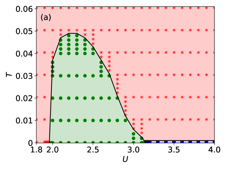
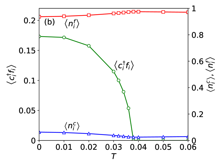
Figure 3: (Color online) (a) Calculated finite-temperature phase diagram of the EFKM as a function of $U$, where the region $\langle c_{i}^{\dagger}f_{i}\rangle\neq 0$ is indicated by the green circles. We use the cluster of $L=7$ and assume $D=1$. (b) Calculated temperature dependence of the order parameter $\langle c_{i}^{\dagger}f_{i}\rangle$ and numbers of electrons in the $c$ and $f$ orbitals $\langle n_{i}^{c}\rangle$ and $\langle n_{i}^{f}\rangle$. We use the cluster of $L=7$ and assume $U=2.6$ and $D=1$.

Next, let us discuss the finite-temperature phase diagram of the EFKM. The calculated result is shown in Fig. 3(a) as a function of $U$ at $D=1$. We find that a dome-like shape of the EI phase actually occurs as a function of $U$ at $2\lesssim U\lesssim 3.2$, which is between the BI (at $3.2\lesssim U$) and SM (at $U\lesssim 2$) phases. Thus, the finite-temperature phase transition actually occurs at $T=T_{c}$, where the value of $T_{c}$ is found to be rather low. Although we may point out on the one hand that the finite-temperature phase transition does not occur in pure 1D systems due to thermal and quantum fluctuations, we may argue on the other hand that any mean-field-type treatment of quantum systems should provide a finite-temperature phase transition, the $T_{c}$ of which may well be low if partial inclusion of quantum fluctuations is made by, e.g., the CMFT as in the present case. The obtained value of $T_{c}$, therefore, does not have a quantitative significance unless the weak three-dimensionality in the real system is introduced explicitly via the realistic interchain coupling parameters, thereby making a quantitative calculation. We should, however, note that the properties of the model above $T_{c}$ can be discussed in the framework of the present CMFT approach, as we will see below.

The calculated temperature dependence of the order parameter and numbers of electrons in the $c$ and $f$ orbitals is shown in Fig. 3(b). We find that the system undergoes a continuous (or second-order) phase transition, as is evident in the behavior of $\langle c_{i}^{\dagger}f_{i}\rangle$. We also find that the value of $\langle n_{i}^{c}\rangle$ ($\langle n_{i}^{f}\rangle$) increases (decreases) with decreasing temperature below $T_{c}$ due to the excitonic condensation (or spontaneous $c$-$f$ hybridization) although the change across the phase transition is rather small.

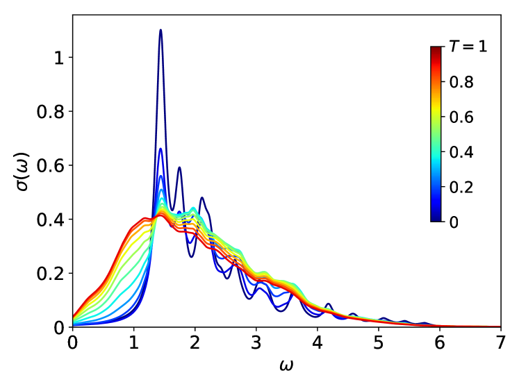
Figure 4: (Color online) Calculated temperature dependence of the optical conductivity spectrum $\sigma(\omega)$. We use the cluster of $L=7$ and assume $U=2.5$ and $D=1$. The broadening parameter of the spectra is set to $\eta=0.1$.

Finally, let us discuss the temperature dependence of the excitation spectra of the EFKM; in particular, we calculate the optical conductivity and single-particle spectra, which we will compare with experiments on Ta₂NiSe₅. The optical conductivity spectrum $\sigma(\omega)$ may be defined as

$$\sigma(\omega)=\omega\,(1-e^{-\beta\omega})\,I(\omega),$$

$$I(\omega)=\frac{1}{\pi}\mathrm{Im}\,Z^{-1}\sum_{m,n}e^{-\beta E_{m}}\frac{\big{|}\langle\Psi_{m}\big{|}\,d\,\big{|}\Psi_{n}\rangle\big{|}^{2}}{\omega-i\eta+E_{m}-E_{n}}$$ (5)

with the dipole operator $d=-e\sum_{l=1}^{L}l\,\big{(}c_{l}^{\dagger}c_{l}+f_{l}^{\dagger}f_{l}-1\big{)}$, where $E_{m}$ and $\Psi_{m}$ are the eigenvalue and eigenstate of the Hamiltonian, respectively [29]. The single-particle spectrum may similarly be defined by replacing $d$ in Eq. (5) with either $c_{k}$ ($f_{k}$) or $c_{k}^{\dagger}$ ($f_{k}^{\dagger}$) with momentum $k$, thereby simulating the angle-resolved photoemission or inverse photoemission spectrum $A(k,\omega)$. Below, we choose $k$ as a central site of the cluster in real space, to calculate the angle-integrated spectrum.

The calculated results for the optical conductivity spectrum $\sigma(\omega)$ is shown in Fig. 4, which may be compared with experiment for Ta₂NiSe₅; see Fig. 3 of Ref. [30] and Fig. 2(c) of Ref. [31]. In our previous paper [11], we have confirmed that the main peak at $\omega\simeq 0.4$ eV in the observed optical conductivity spectrum originates from the repulsive interaction between electrons on the $c$ and $f$ orbitals at the same site, which is nothing but the attractive interaction between an electron on the $c$ orbital and a hole on the $f$ orbital at the same site. In other words, the main peak in the optical conductivity spectrum is caused by the electron-hole pair formation. Here, we moreover confirm that, in both theory and experiments [30, 31], the main peak remains robust even above $T_{c}$, where the pairs are not condensed. Then, it seems quite natural to assume that the main peak of the optical conductivity reflects the preformed pair states of the system.

We find that the temperature-induced spectral weight transfer, observed experimentally in Ta₂NiSe₅ [30, 31], is qualitatively well reproduced by our calculation; i.e., the spectral weight is transferred from high-frequency to low-frequency regions by increasing temperature. We should note that the change in the spectral features at $T_{c}$ is unnoticeably small, which is also consistent with experiments, where virtually no discontinuous changes occur at $T_{c}$ [30, 31]. The behavior of this peak thus illustrates the preformed electron-hole pair state in Ta₂NiSe₅, which appears even far above $T_{c}$.

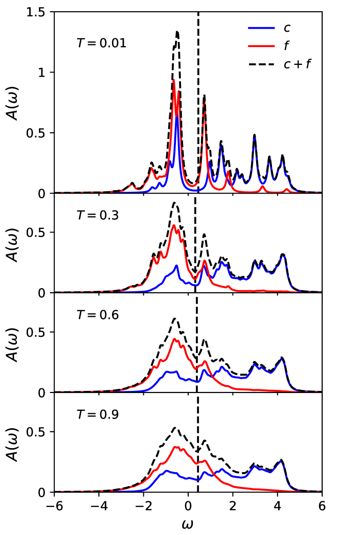
Figure 5: (Color online) Calculated temperature ($T$) dependence of the $k$-integrated single-particle spectra $A(\omega)$, where $c$ and $f$ contributions are shown separately., together with the total spectral weight $c+f$. The vertical line indicates the Fermi level. We use the cluster of $L=7$ and assume $U=2.5$ and $D=1$. The broadening parameter of the spectra is set to $\eta=0.1$.

The calculated results for the $k$-integrated single-particle spectrum $A(\omega)$ are shown in Fig. 5, where we find that the band-gap feature observed at $T=0$ essentially remains even far above $T_{c}$ as a pseudogap-like structure, indicating that the electron-hole pairs survive robustly. The temperature dependence of the angle-resolved photoemission spectra observed experimentally [9] are consistent with our calculated results.

Thus, the preformed pair state in the strong-coupling regime of excitonic insulators manifests itself in both the optical conductivity and single-particle spectra.

In summary, we studied the excitonic condensation in the 1D EFKM at finite temperature based on the CMFT approach. We obtained the ground-state and finite-temperature phase diagrams of the model using the grand canonical exact-diagonalization analysis of small clusters with the SSD function, whereby the unphysical temperature and parameter dependence of the results was suppressed. We also presented the temperature dependence of the optical conductivity and single-particle spectra of the model and compared them with experiments on Ta₂NiSe₅. We thus discussed how the preformed pair state appears in the strong-coupling regime of the EI. We hope that more quantitative analyses of the experimental data will be made in future based on more realistic models [32, 33] and more powerful computational techniques,[34, 35] to reveal the entire aspects of the excitonic insulator states in the strong-coupling regime.

- [1] N. F. Mott, Philos. Mag. 6, 287 (1961).
- [2] D. Jérome, T. M. Rice, and W. Kohn, Phys. Rev. 158, 462 (1967).
- [3] B. I. Halperin and T. M. Rice, Rev. Mod. Phys. 40, 755 (1968).
- [4] J. Kuneš, J. Phys. Condens. Matter 27, 333201 (2015).
- [5] Y. Ohta, T. Kaneko, and K. Sugimoto, Solid State Physics 52, 119 (2017) [in Japanese].
- [6] Y. Wakisaka, T. Sudayama, K. Takubo, T. Mizokawa, M. Arita, H.Namatame, M.Taniguchi,N. Katayama, M. Nohara, and H. Takagi, Phys. Rev. Lett. 103, 026402 (2009).
- [7] Y. Wakisaka, T. Sudayama, K. Takubo, T. Mizokawa, N. L. Saini, M. Arita, H. Namatame, M. Taniguchi, N. Katayama, M. Nohara, and H. Takagi, J. Supercond. Nov. Magn. 25, 1231 (2012).
- [8] T. Kaneko, T. Toriyama, T. Konishi, and Y. Ohta, Phys. Rev. B 87, 035121 (2013); 87, 199902 (2013).
- [9] K. Seki, Y. Wakisaka, T. Kaneko, T. Toriyama, T. Konishi, T. Sudayama, N. L. Saini, M. Arita, H. Namatame, M. Taniguchi, N. Katayama, M. Nohara, H. Takagi, T. Mizokawa, and Y. Ohta, Phys. Rev. B 90, 155116 (2014).
- [10] A. N. Kozlov and L. A. Maksimov, Sov. Phys. JETP 21, 790 (1965).
- [11] K. Sugimoto, S. Nishimoto, T. Kaneko, and Y. Ohta, Phys. Rev. Lett. 120, 247602 (2018).
- [12] B. Zenker, D. Ihle, F. X. Bronold, and H. Fehske, Phys. Rev. B 81, 115122 (2010).
- [13] K. Seki, R. Eder, and Y. Ohta, Phys. Rev. B 84, 245106 (2011).
- [14] Y. Shibata, S. Nishimoto, and Y. Ohta, Phys. Rev. B 64, 235107 (2001).
- [15] A. F. Albuquerque, D. Schwandt, Hetényi, S. Capponi, M. Mambrini, and A. M. Läuchli, Phys. Rev. B 84, 024406 (2011).
- [16] W. Brzezicki, J. Dziarmaga, and A. M. Oleś, Phys. Rev. Lett. 109, 237201 (2012).
- [17] R. Suzuki and A. Koga, JPS Conf. Proc. 3, 016005 (2014).
- [18] D. Gotfryd, J. Rusnačko, K. Wohlfeld, G. Jackeli, J. Chaloupka, and A. M. Oleś, Phys. Rev. B 95, 024426 (2017).
- [19] A. Singhania and S. Kumar, Phys. Rev. B 98, 104429 (2018).
- [20] C. Hotta and N. Shibata, Phys. Rev. B 86, 041108(R) (2012).
- [21] C. Hotta, S. Nishimoto, and N. Shibata, Phys. Rev. B 87, 115128 (2013).
- [22] L. M. Falicov and J. C. Kimball, Phys. Rev. Lett. 22, 997 (1969).
- [23] There is a variety of the mean-field replacements: (i) several exchange bonds in the periodic finite-size cluster are replaced by the mean-field bonds [15], (ii) an open finite-size cluster is surrounded by the mean-field sites [18], and (iii) only one bond is replaced by the mean-field bond in the periodic finite-size chain [14, 19], etc. Thus, there is some arbitrariness in the ways of introducing the mean-fields in CMFT. In a broad sense, the CMFT can be defined as a self-consistent determination of the mean-fields to minimize the total energy of a cluster where a part of sites and/or bonds are replaced by the mean-field sites and/or bonds.
- [24] We note that the well-known Mermin-Wagner theorem [Phys. Rev. Lett. 17, 1133 (1966)] is apparently violated here.
- [25] S. Ejima, T. Kaneko, Y. Ohta, and H. Fehske, Phys. Rev. Lett. 112, 026401 (2014).
- [26] U. Schollwöck, DMRG: Ground States, Time Evolution, and Spectral Functions in Emergent Phenomena in Correlated Matter Vol. 3, edited by E. Pavarini, E. Koch, and U. Schollwöck (Verlag des Forschungszentrum Jülich, Jülich, 2013).
- [27] K. Okunishi and T. Nishino, Phys. Rev. B 82, 144409 (2010).
- [28] A. N. Kocharian and J. H. Sebold, Phys. Rev. B 53, 12804 (1996).
- [29] F. Gebhard, K. Bott, M. Scheidler, P. Thomas, and S. W. Koch, Philos. Mag. B 75, 1 (1997).
- [30] Y. F. Lu, H. Kono, T. I. Larkin, A. W. Rost, T. Takayama, A. V. Boris, B. Keimer, and H. Takagi, Nat. Commun. 8, 14408 (2017).
- [31] T. I. Larkin, A. N. Yaresko, D. Pöpper, K. A. Kikoin, Y. F. Lu, T. Takayama, Y.-L. Mathis, A. W. Rost, H. Takagi, B. Keimer, and A. V. Boris, Phys. Rev. B 95, 195144 (2017).
- [32] K. Sugimoto and Y. Ohta, Phys. Rev. B 94, 085111 (2016).
- [33] G. Mazza, M. Rösner, L. Windgätter, S. Latini, H. Hübener, A. J. Millis, A. Rubio, and A. Georges, arXiv:1911.11835.
- [34] K. Seki, T. Shirakawa, and S. Yunoki, Phys. Rev. B 98, 205114 (2018).
- [35] H. Nishida, R. Fujiuchi, K. Sugimoto, and Y. Ohta, J. Phys. Soc. Jpn. 89, 023702 (2020).