Supervised Dimensionality Reduction and Visualization using Centroid-encoder

Abstract

Visualizing high-dimensional data is an essential task in Data Science and Machine Learning. The Centroid-Encoder (CE) method is similar to the autoencoder but incorporates label information to keep objects of a class close together in the reduced visualization space. CE exploits nonlinearity and labels to encode high variance in low dimensions while capturing the global structure of the data. We present a detailed analysis of the method using a wide variety of data sets and compare it with other supervised dimension reduction techniques, including NCA, nonlinear NCA, t-distributed NCA, t-distributed MCML, supervised UMAP, supervised PCA, Colored Maximum Variance Unfolding, supervised Isomap, Parametric Embedding, supervised Neighbor Retrieval Visualizer, and Multiple Relational Embedding. We empirically show that centroid-encoder outperforms most of these techniques. We also show that when the data variance is spread across multiple modalities, centroid-encoder extracts a significant amount of information from the data in low dimensional space. This key feature establishes its value to use it as a tool for data visualization.

Keywords Data Science, Machine Learning, supervised dimension reduction, centroid-encoder, autoencoder, variance

1 Introduction

Visualization of data is the process of mapping points in dimensions greater than three down to two or three dimensions, providing a window into high-dimensions so that they can be seen and interpreted. The ability to see in high-dimensions can assist data explorers in many ways, including the identification of experimental batch effects, data separability, and class structure. Principal component analysis [1, 2] continues to be one of the most widely used methods for data visualization over one hundred years after its initial discovery [3]. Nonetheless, PCA often produces ambiguous results, in some cases collapsing distinct classes into overlapping regions in the setting where class labels are available. It is tempting to incorrectly infer from this that the data is not separable, even nonlinearly, in higher dimensions.

Nonlinear extensions to PCA were originally introduced to address the limitations of optimal linear mappings [4, 5, 6], also see [7] for additional early references and details. These papers provided the first applications of autoencoder neural networks where data sets are nonlinearly mapped to themselves. This is accomplished by first unfolding them in higher dimensions before passing through a bottleneck layer of a reduced dimension where data visualization is typically done. In the process of nonlinear dimension reduction, novel latent or hidden features which are an amalgamation of the observables, may be discovered. A theoretical insight into these algorithms is provided by Whitney’s theorem from differential geometry that connects autoencoders to manifold learning [8, 9]. Fundamental innovations were proposed to these ideas in the setting of deep networks that made their application far more effective [10, 11].

The development of tools for data visualization is predicated by the design of the objective function and whether it incorporates class label information, i.e., is it supervised or unsupervised. The objective function encodes the goals of the dimension reduction, i.e., what important information about the data is to be captured. This might be geometric or topological structure (shape), neighborhood relationships, or descriptive statistics such as class distribution data when data class labels are available.

This paper concerns the integration of label information to the nonlinear autoencoder reduction process for the purposes of data visualization. Here we develop and comparatively evaluate this centroid-encoder (CE) algorithm designed for the analysis of labeled data. While standard autoencoders map the identity on points, centroid-encoders map points to their centroids while passing through a low-dimensional representation. This approach serves to provide a low-dimensional encoding for visualization while ensuring that elements with the same label retain their class structure. The smoothness of mapping functions ensures that a similar behavior is captured at the centroid-encoder bottleneck layer.

In this paper, we analyze centroid-encoder and compare its performance with other methods. The article is organized as follows: In Section 2, we review related work, both supervised and unsupervised. In Section 3, we discuss the autoencoder neural network for nonlinear data reduction. In Section 4, we present modifications to the autoencoder that result in centroid encoding. In Section 5, we present the training algorithm employed in this paper. In Section 6, we illustrate the application of CE to a range of bench-marking data sets taken from the literature. In Section 7, we analyze these results and conclude in Section 8.

2 Related Work

Data reduction for visualization has a long history and remains an area of active research. We describe the literature relating to unsupervised and supervised methods where we assume data class labels are unavailable and available, respectively.

2.1 Unsupervised Methods

Principal Components Analysis is often the first (and last) tool used for visualization of unlabeled data and is designed to retain as much of the statistical variance as possible [1, 2], see also [12]. Equivalently, PCA minimizes mean-square approximation error as well as Shannon’s entropy [13]. Self-organizing mappings (SOMs) learn nonlinear topology-preserving transformations that map data points to centers that are then mapped to the center indices. SOMs have been widely used in data visualization, having been cited over 20,000 times since their introduction [14].

Another class of methods uses interpoint distances as the starting point for data reduction and visualization. For example, Multidimensional Scaling is a spectral method that computes a point configuration based on the computation of the eigenvectors of a doubly centered distance matrix [15]. The goal of the optimization problem behind MDS is to determine a configuration of points whose Euclidean distance matrix is optimally close to the prescribed distance matrix. A related approach, known as Isomap, applies MDS to approximate geodesic distances computed numerically from data on a manifold [16]. Laplacian eigenmaps is another popular spectral method that uses distance matrices to reduce dimension and conserve neighborhoods [17]. These spectral methods belong to a class of techniques referred to as manifold learning algorithms; see also locally linear embedding [18], stochastic neighbor embedding [19], and maximum variance unfolding [20].

The technique t-distributed stochastic neighbor embedding [21], an extension of SNE, was developed to overcome the data crowding or clumping problem often observed with manifold learning methods and is currently a popular method for data visualization. More recently, the uniform manifold approximation and projection (UMAP) algorithm has been proposed, which uses Riemannian geometry and fuzzy simplicity sets to create a low-dimensional and locally uniformly distributed embedding of the data [22]. It has been reported that the algorithm has a better run time than t-SNE and offers compelling visualizations.

Note that these spectral methods including MDS, Laplacian Eigenmaps and UMAP compute embeddings based on solving an eigenvector problem requiring the entire data set. Such methods do not actually create mappings that can be applied to reduce the dimension of new data points without repeating the computation or resorting to the use of landmarks [23]. This, in contrast to methods such as PCA, SOM and autoencoders that serve as mappings for streaming data.

2.2 Supvervised Methods

Fisher’s linear discriminant analysis (LDA) reduces the dimension of labeled data by simultaneously optimizing class separation and within-class scatter [24, 25]. Both LDA and PCA are linear methods in that they construct optimal projection matrices, i.e., linear transformations for reducing the dimension of the data.

It is, in general, possible to add labels to unsupervised methods to create their supervised analogues. A heuristic-based supervised PCA model first selects important features by calculating correlation with the labels and then applies standard PCA of the chosen feature set [26]. Another supervised PCA technique, proposed by Barshan et al. [27], uses a Hilbert-Schmidt independence criterion to compute the principal components which have maximum dependence on the labels. Colored maximum variance unfolding [28], which is the supervised version of MVU, is capable of separating different new groups better than MVU and PCA.

The projection of neighborhood component analysis [29] produces a better coherent structure in two-dimensional space than PCA on several UCI data sets. Parametric embedding [30], which embeds high-dimensional data by preserving the class-posterior probabilities of objects, separates different categories of Japanese web pages better than MDS. Optimizing the NCA objective on a pre-trained deep architecture, Salakhutdinov et al. [31] achieved $1\%$ error rate on MNIST test data with 3-nearest neighbor classifier on 30-dimensional feature space. Min et al. proposed to optimize the NCA and maximally collapsing metric learning [32] objective using a Student t-distribution on a pre-trained network [33]. Their approach yielded promising generalization error using a 5-nearest neighbor classifier on MNIST and USPS data on two-dimensional feature space. Neighbor retrieval visualizer [34] optimizes its cost such that the similar objects are mapped close together in embedded space. Its supervised variant uses the class information to produce the low dimensional embedding. NeRV and its supervised counterpart were reported to outperform some of the state-of-the-art dimension reduction techniques on a variety of datasets.

Supervised Isomap [35], which explicitly uses the class information to impose dissimilarity while configuring the neighborhood graph on input data, has a better visualization and classification performance than Isomap. A supervised method using Local Linear Embedding has been proposed by [36]. [37] have suggested a Laplacian eigenmap based supervised dimensionality reduction technique. Stuhlsatz et al. proposed a generalized discriminant analysis based on classical LDA [38], which is built on deep neural network architecture. Min et al. proposed a shallow supervised dimensionality reduction technique where the MCML objective is optimized based on some learned or precomputed exemplars [39]. Although UMAP is originally presented as an unsupervised technique, its software package includes the option to build a supervised model . UMAP is available in Python’s Scikit-learn package [40].

Autoencoder neural networks are the starting point for our approach and are described in the next section. In a preliminary biological application, centroid-encoder (CE) was used to visualize the high-dimensional pathway data [41].

3 Autoencoder Neural Networks

An autoencoder is a dimension reducing mapping that has been optimized to approximate the identity on a set of training data [42, 7, 43]. The mapping is modeled as the composition of a dimension reducing mapping $g$ followed by a dimension increasing reconstruction mapping $h$, i.e.,

$$f(x)=h(g(x))$$

where the encoder $g$ is represented

$$g:U\in\mathbb{R}^{n}\rightarrow V\in\mathbb{R}^{m}$$

and the decoder $h$ is represented

$$h:V\in\mathbb{R}^{m}\rightarrow U\in\mathbb{R}^{n}$$

The construction of $g$ and $h$, and hence $f$, is accomplished by solving the unconstrained optimization problem

$$\underset{\theta}{\text{minimize}}\;\;\sum_{i}\|x^{i}-f(x^{i};\theta)\|_{2}^{2}$$ (1)

for a given set of points $X=\{x^{1},x^{2},x^{3},...\}$. Hence, the autoencoder learns a function $f$ such that $f(x^{i};\theta)\approx x^{i}$ where $\theta$ is the set of model parameters that is found by solving the optimization problem. The encoder map $g$ takes the input $x^{i}$ and maps it to a latent representation

$$y^{i}=g(x^{i})\in V\subset\mathbb{R}^{m}$$

In this paper we are primarily concerned with visualization so we take $m=2$. The decoder ensures that the encoder is faithful to the data point, i.e., it serves to reconstruct the reduced point to its original state

$$x^{i}\approx h(y^{i})$$

The parameters $\theta$ are learned by using error backpropagation [44, 45]. The details for using multi-layer perceptrons for training autoencoders can be found in [7].

If we restrict $g$ and $h$ to be linear transformations then [46] showed that autoencoder function learns the same subspace of PCA. The nonlinear autoencoder has been proposed as a nonlinear version of PCA [4, 5]. If we restrict $g$ to be linear and allow $h$ to be nonlinear then the autoencoder fits into the blueprint of Whitney’s theorem for manifold embeddings [8, 9]. Topologically sensitive nonlinear reduction use, e.g., topological circle or sphere encoding neurons [47, 48, 49] to capture shape in data. The use of shallow architectures was partly motivated by the theoretical result that a neural network with one hidden layer is a universal approximator by [50, 51].

A probabilistic pre-training approach, known as Restricted Boltzmann Machine (RBM), was introduced [11, 10], which initializes the network parameters near to a good solution followed by a nonlinear refinement to further fine-tune the parameters. This break-through opened the window of training neural networks with many hidden layers. Since then deep neural networks (DNN) architecture has been employed to train autoencoders. The pre-training approach was extended further to continuous values by [43, 52]. Several other deep autoencoder based model were also proposed to extract sparse features [53, 54]. The method of denoising autoencoder [55] was introduced to learn latent features by reconstructing an input from it noisy version. Autoencoders can also be trained by stacking multiple convolutional layers as described by [56, 57, 58]. A comprehensive description of autoencoders and their variants can be found in [59, chap. 14].

4 The Centroid-Encoder

The autoencoder neural network does not employ any label information related to the classes of the data. Here we propose a form of supervised autoencoder that exploits label information. The centroid-encoder (CE) is trained by mapping data through a neural network with the architecture of an autoencoder, but the learning target of any point is not that actual point, rather the mean of points in the associated class. So CE does not map the identity, now the target points in the image of the map are the centroids of the data in the ambient space. Centroid-encoder is a nonlinear parametric map ($f_{\theta}$ where $\theta$ is the set parameters) which minimizes the within-class variance by mapping all the samples of a class/category to its centroid.

4.1 Centroid-Encoder Backpropagation

Consider an $M$-class data set with classes denoted $C_{j},j=1,\dots,M$ where the indices of the data associated with class $C_{j}$ are denoted $I_{j}$. We define centroid of each class as

$$c_{j}=\frac{1}{|C_{j}|}\sum_{i\in I_{j}}x^{i}$$

$|C_{j}|$ is the cardinality of class $C_{j}$. The centroid-encoder is trained by determining a mapping $f=h\circ g$ with input-output pairs

$$\{x^{i},c_{j}\}_{i=1}^{N}$$

where $c_{j}$ is the target center for data point $x^{i}$, i.e., $i\in I_{j}$. Thus, unlike autoencoder, which maps each point $x^{i}$ to itself, centroid-encoder will map each point $x^{i}$ to its class centroid $c_{j}$

$$c_{j}\approx f(x^{i})$$

while passing the data through a bottleneck layer of dimension $m$ to provide the reduced point $g(x^{i})$. The cost function of centroid-encoder is defined as

$$\mathcal{L}_{ce}(\theta)=\frac{1}{2N}\sum^{M}_{j=1}\sum_{i\in I_{j}}\|c_{j}-f(x^{i};\theta))\|^{2}_{2}$$ (2)

This cost is also referred to as the distortion error ([60]). The network parameters ($\theta$) are trained using the error backpropagation appropriately modified for the centroid targets. We can connect this to the learning procedure for autoencoders by first writing

$$\mathcal{L}_{ce}(\theta)=E(f(\theta))$$

where the $f(\theta)$ is identical for autoencoders and centroid-encoders. Then, applying the chain rule, we have

$$\frac{\partial{\mathcal{L}_{ce}(\theta)}}{\partial\theta_{i}}=\frac{\partial E}{\partial f}\frac{\partial f}{\partial\theta_{i}}$$

where the term $\frac{\partial f}{\partial\theta_{i}}$ is the same as for autoencoders and $\theta_{i}$ is the $i$th component of the parameter vector $\theta$. The new term $\frac{\partial E}{\partial f}$ is readily calculated to be

$$\frac{\partial E}{\partial f}=\frac{1}{N}\sum^{M}_{j=1}\sum_{i\in I_{j}}(f(x^{i},\theta)-c_{j})$$ (3)

5 The Training Algorithm

The training is very similar to that of an autoencoder and the steps are described in Algorithm 1. As with autoencoders, the centroid-encoder is a composition of two maps $f(x)=(h\circ g)(x)$. For visualization, we train a centroid-encoder network using a bottleneck architecture, meaning that the dimension of the image of the map $g$ is 2 or 3.

1

Input Data: Labeled Data ${\{x^{i}\}}^{N}_{i=1}\,\in{\mathbb{R}}^{n},\,\,I_{j}$ index set of class $C_{j}.$ User defined parameters training epoch $n\_epochs$ and visualization dimension $m$.

Output Data: Bottleneck layer $y^{i}=g(x^{i})$; Output layer $h(y^{i}),i=1,\dots,N.$

Nonlinear function: $f:{\mathbb{R}}^{n}\to{\mathbb{R}}^{n}$ where $f=h\circ g$.

Result: Nonlinear embedding of data in $m$ dimensions.

Initialization: Calculate the class centroids $c_{j}=\frac{1}{|C_{j}|}\sum_{i\in I_{j}}{x^{i}},j=1,\dots,M$.

Define: Centroid-encoder output error $E=\frac{1}{2N}\sum_{j}\sum_{i\in I_{j}}\|c_{j}-f(x^{i},\theta)\|^{2}_{2}$

2

3for $k=1$ to $n\_epochs$ do

4      

5      Update parameters $\theta$ of centroid-encoder.  

6 end for

Algorithm 1 Supervised Nonlinear Centroid-Encoder.

5.1 Pre-training Centroid-encoder

Here we describe the pre-training strategy of centroid-encoder. We employ a technique we refer to as pre-training with layer-freeze, i.e., pre-training is done by adding new hidden layers while mapping samples of a class to its centroid; see Figure 1. In this approach, weights of hidden layers are learned sequentially. The algorithm starts by learning the parameters of the first hidden layer using standard backpropagation. Then the second hidden layer is added in the network with weights initialized randomly. At this point, the associated parameters of the first hidden layer are kept frozen. Now the weights of the second hidden layer are updated using backpropagation. We repeat this step until pre-training is done for each hidden layer. Once pre-training is complete, we do an end-to-end fine-tuning by updating the parameters of all the layers at the same time. It’s noteworthy that our pre-training approach is different than the greedy layer-wise pre-training proposed by [11] and [43, 52]. The unsupervised pre-training of Hinton et al. and Bengio et al. uses the activation of the $l^{th}$ hidden layer as the input for the $(l+1)^{th}$ layer. In our approach, we used the original input-output pair $(x^{i},c_{j})$ to pre-train each hidden layer. As we use the labels to calculate the centroids $c_{j}$, so our pre-training is supervised. In the future, we would like to explore the unsupervised pre-training in the setup of centroid-encoder.

Figure 1: Pre-training a deep centroid-encoder by layer-freeze approach. In the first step, a centroid-encoder with the first hidden layer is pre-trained (left diagram). The pre-trained weights are ($W_{1},\widetilde{W_{1}}$). In the next step, a new hidden layer is added by extending the network architecture. After that, the weights ($W_{2},\widetilde{W_{2}}$) associated with the new hidden layer are updated while keeping the other weights ($W_{1},\widetilde{W_{1}}$) fixed. This process is repeated to add more hidden layers.

6 Classification and Visualization Experiments

We select three suites of data sets from the literature with which we conduct three bench-marking experiments comparing centroid-encoder with a range of other supervised dimension reduction techniques. We describe the details of the data sets in Section 6.1. In Section 6.2, we describe the comparison methodology and present the results of the experiments in Section 6.3.

Experiment 1: The first bench-marking experiment is conducted on the widely studied MNIST and USPS data sets (see Section 6.1 for details). In this experiment we compare CE with the following methods: autoencoder, nonlinear NCA [31], supervised UMAP [22], GerDA [38], HOPE [39], parametric t-SNE [61], t-distributed NCA [33] and t-distributed MCML [33], and supervised UMAP. Parametric t-SNE is a DNN based model with RBM pre-training, where the objective of t-SNE is used to update the model parameters (hence parametric t-SNE). Although it is an unsupervised method, we included it as t-SNE has become a baseline model to compare visualization. We also included autoencoder as it is widely used for data visualization. We implemented nonlinear-NCA in Python, and we used the scikit-learn [40] package to run supervised UMAP. For the rest of the methods, we took the published results for comparison.

Experiment 2: We conducted the second experiment on Phoneme, Letter, and Landsat data sets (see Section 6.1 for details). In this case, we compared CE with the following techniques: supervised neighbor retrieval visualizer (SNeRV) by [34], multiple relational embedding (MRE) by [62], colored maximum variance unfolding (MUHSIC) by [28], supervised isomap (S-Isomap) by [35], parametric embedding (PE) by [30] and neighborhood component analysis (NCA) by [29]. We didn’t implement these models; instead, we used the published results from [34]. On the Landsat data set, we ran UMAP and SUMAP along with the methods as mentioned above.

Experiment 3: For the third experiment, we compared the performance of centroid-encoder with supervised PCA (SPCA), and kernel supervised PCA (KSPCA) on the Iris, Sonar, and a subset of USPS dataset (details of these dataset are given in Section 6.1). We implemented SPCA and KSPCA in Python following [27].

6.1 Data Sets

Here we provide a brief description of the data sets used in the bench-marking experiments.

MNIST Digits: This is widely used collection of digital images of handwritten digits (0..9) with separate training (60,000 samples) and test set (10,000 samples). Each sample is a grey level image consisting of 1-byte pixels normalized to fit into a 28 x 28 bounding box resulting in vecced points in $\mathbb{R}^{784}$.

USPS Data: A data set of handwritten digits ($0\dots 9$), where each element is a 16x16 image in gray-scale resulting in vecced points in $\mathbb{R}^{256}$. Each of the ten classes has 1100 digits for a total of 11,000 digits.

Phoneme Data: This data set is created from Finish speech recorded continuously from the same speaker. A 20-dimensional vector represents each phoneme. The data set consists of 3924 number of samples distributed over 13 classes. The data set is taken from the LVQ-PAK software package.

Letter Recognition Data: Available in the UCI Machine Learning Repository [63], this data set is comprised of 20,000 samples where each element represents an upper case letter of the English alphabet A to Z selected from twenty different fonts. Each sample is randomly distorted to produce a unique representation that is converted to 16 numerical values and 26 classes.

Landsat Satellite Data: This data set consists of satellite images with four different spectral bands. Given the pixel values of a 3x3 neighborhood, the task is to predict the central pixel of each 3x3 region. Each sample consists of 9-pixel values from 4 different bands, which makes the dimension 36. There are six different classes and 6435 samples. The data set is also available in UCI Machine Learning Repository [63].

Iris Data: The UCI Iris data set [63] is comprised of three classes and is widely used in the Machine Learning literature. Each class has 50 samples and, each sample has four features.

Sonar Data: This UCI data set [63] has two classes: mine and rock. Each sample is represented by a 60 dimensional vector. The mine class has 111 patterns, whereas the rock category has 97 samples.

In the next section we describe the methodology used to compare the low-dimensional embedding of CE with other methods on the data sets described above.

6.2 Methodology

To objectively compare the performance of CE with other techniques in the literature, we employ a standard class prediction error on the two-dimensional visualization domain. As we are comparing supervised methods, we restrict our attention to the generalization performance as measured by a test data set.

The class prediction error is defined as

$$Error\;(\%)=\frac{100}{N}\sum^{N}_{i=1}I[l_{i}\neq f(\tilde{x_{i}})]$$ (4)

Here $N$ is total number of test samples, $l_{i}$ is the true label of the $i^{th}$ test sample, and $f$ is a classification function which returns the predicted label of the embedded test sample $\tilde{x_{i}}$. Here $I$ denotes the indicator function, which has the value 1 if the argument is true (label incorrect), and 0 otherwise (label correct).

A common choice of $f$ for bench-marking algorithms in the supervised visualization literature is the $k$-nearest neighbor (k-NN) classifier [29, 34, 61, 33]. Thus, the evaluation proceeds as follows: for each method divide the data into training and testing sets; train the model on the training set and then map the test set through the trained model to get the low dimensional (2D) representation. Finally, classify each test point in the 2D visualization space by k-NN algorithm. The prediction error indicates the percentage of wrongly classified samples on the test data and is an objective measure of the quality of the visualization. A low error rate suggests that the samples from the same class are close together in the visualization space.

Like autoencoder, centroid-encoder is a model based on deep architecture whose performance varies based on network topology. In addition to network architecture, both the models require the following hyper-parameters: learning rate, mini-batch size, and weight decay constant. As with all neural network learning algorithms, these parameters need to be tuned to yield optimal performance. The details of the training procedure vary by data set. We used subsets of the training data (3000 and 30,000 for USPS and MNIST respectively), picked randomly, and ran 10-fold cross-validation to determine the network architecture and hyper-parameters. On MNIST, we trained CE on the entire training set and then used the test data to calculate class prediction error using a $k$-NN ($k=5$) algorithm. On USPS data, we followed the strategy of [33], where we randomly split the entire data set into a training set of 8000 samples and a test set consisting of 3000 samples. After building the model on training samples, we used the test set to calculate the error using $k$-NN with $k$=5. In both cases, we repeat the experiment 10 times and report the average error rate with standard deviation.

The supervised UMAP (S-UMAP) and nonlinear NCA (NNCA), also require the tuning of hyper-parameters. For NNCA, we used the architecture input dimension $d\rightarrow 500\rightarrow 500\rightarrow 2000\rightarrow 2$ as proposed by [33]; we also followed the same pre-training and fine-tuning steps described there. The algorithm S-UMAP requires two hyper-parameters including, the number of neighbors ($n\_neighbors$) and minimum distance ($min\_dist$) allowed between the points in reduced space. On the MNIST and USPS, we used 10-fold cross-validation on a randomly-selected subset of training data (3000 and 30,000 for USPS and MNIST respectively) to optimize these parameters.

On Phoneme, Letter, and Landsat data, our experimental setup is similar to that of [34]. We randomly selected 1500 samples from each dataset and ran 10-fold cross-validation. We picked the hyper-parameters (network architecture, learning rate, mini-batch size, weight decay) by running 10-fold internal cross-validation on the training set. After choosing the model parameters, we trained the model with the full training data and calculated the error rate using $k$-NN ($k$=5) on the holdout test set. Once all the 10 test sets are evaluated, we reported the average test error with standard deviation.

Dataset	Dimensionality	No. of Classes	No. of Training	No. of Test
			Samples	Samples
MNIST	784	10	60,000	10,000
USPS	256	10	8000	3000
Phoneme	20	13	1,350	150
Letter	16	26	1,350	150
Landsat	36	6	1,350	150
Iris	4	3	105	45
Sonar	60	2	146	62
USPS 1000	256	10	700	300

Table 1: Details of data sets along with the sample count of training and test set used in the visualization experiments.

We followed the experimental setup of [27] in the last experiment, where we compared centroid-encoder with supervised PCA (SPCA) and kernel supervised PCA (KSPCA). Each of the three data sets (Iris, Sonar, USPS) is split randomly into training and test by the ratio of 70:30. After training the models, the generalization error is calculated on the test set using $k$-NN ($k$=5). We repeat the experiment 25 times and report the average error with the standard deviation for all three data sets. For the USPS set, we randomly picked 1000 cases and used that subset for our experiment, as done by [27]. Among the three models, centroid-encoder and KSPCA require hyper-parameters. For KSPCA we apply RBF kernel on data and delta kernel on labels, as recommended by Barshan et al. The delta kernel doesn’t require any parameter, whereas the RBF kernel needs the parameter $\gamma$ (width of the Gaussian) which was picked by running 10-fold internal cross-validation on the training set. Table 1 gives the sample count of training and test sets of each data set along with other relevant information. We used two versions of USPS data: in Experiment 1, we used the entire data set, and in Experiment 3, we used a subset (USPS 1000).

Dataset	Network topology	Activation	Learning	Batch	Weight
		function	rate	size	Decay
MNIST	$d\rightarrow 1000\rightarrow 500\rightarrow 125\rightarrow 2$	tanh	0.0008	512	2e-5
USPS	$d\rightarrow 2000\rightarrow 1000\rightarrow 500\rightarrow 2$	relu	0.001	64	2e-5
Phoneme	$d\rightarrow 250\rightarrow 150\rightarrow 2$	relu	0.01	50	2e-5
Letter	$d\rightarrow 250\rightarrow 150\rightarrow 2$	relu	0.01	50	5e-5
Landsat	$d\rightarrow 250\rightarrow 150\rightarrow 2$	relu	0.01	50	5e-5
Iris	$d\rightarrow 100\rightarrow 2$	relu	0.001	16	2e-5
Sonar	$d\rightarrow 500\rightarrow 250\rightarrow 2$	relu	0.001	16	2e-5

Table 2: Details of network topology and hyper-parameters for CE. The number $d$ is the input dimension of the network and is data set dependent.

To train CE with an optimal number of epochs, we used $10\%$ of training samples as a validation set in all of our visualization experiments. We measure the generalization error on the validation set after every training epochs. Once the validation error doesn’t improve, we stop the training. Finally, we merge the validation set with the training samples and train the model for additional epochs. The model parameters are updated using Adam optimizer ([64]). Table 2 gives the details of network topology and hyper-parameters used in training of CE. We have implemented centroid-encoder in PyTorch to run on GPUs. The implementation is available at: https://github.com/Tomojit1/Centroid-encoder/tree/master/GPU.

In addition to computing the prediction error, we also visualize the two-dimensional embedding of test samples of each model. For centroid-encoder, we plot the bottleneck output of training and test data using Voronoi regions. Here, the bottleneck outputs of training data are used to compute the centroids of each class, which are used to create the Voronoi cells. The test set was then mapped to the reduced space. This visualization approach allows one to see the quality of the CE classification directly.

6.3 Quantitative and Visual Analysis

Now we present the results from a comprehensive quantitative and qualitative analysis across diverse data sets. Note that the primary objective of our assessment is to determine the quality of information obtained from visualization, including class separability, data scatter, and neighborhood structure. Since this assessment is by its very nature subjective, we also employ label information to determine classification rates that provide additional insight into the data reduction for visualization. Computational expense is also an essential factor, and we will see that this is a primary advantage of CE over other methods when the visualizations and error rates are comparable.

6.3.1 MNIST

As shown in Tables 3 (results with pre-training) and 4 (results without pre-training), the models with relatively low error rates for the MNIST data amongst our suite of visualization methods are dt-MCML, dG-MCML, centroid-encoder, and HOPE. The error rate of CE is comparable to the top-performing model dt-MCML and superior to NNCA and supervised UMAP by a margin of $2.1\%$ and $0.84\%$, respectively. Note that methods in the MCML and NCA families require the computation of distance matrix over the data set, making them significantly more expensive than CE, which only requires distance computations between the data of a class and its center. It’s noteworthy that the error of CE is lower than the other non-linear variants of NCA: dt-NCA and dG-NCA. Among all the models, parametric t-SNE (pt-SNE) and autoencoder exhibit the worst performance with error rates on MNIST data are $9.90\%$ and $22.35\%$, respectively. These high error rates are not surprising given these methods do not use label information.

The prediction error of CE with pre-training is relatively low at $2.6\%$, as shown in Table 3 behind the more computationally expensive dt-MCML and dG-MCML algorithms. With no pre-training, the numeric performance of centroid-encoder is statistically equivalent to dt-MCML and HOPE.

Method	Dataset
	MNIST	USPS
Centroidencoder	$2.61\pm 0.09$	$2.91\pm 0.31$
Supervised UMAP	$3.45\pm 0.03$	$6.17\pm 0.23$
NNCA	$4.71\pm 0.57$	$6.58\pm 0.80$
Autoencoder	$22.04\pm 0.78$	$16.49\pm.91$
dt-MCML	2.03	$\textbf{2.46}\pm\textbf{0.35}$
dG-MCML	$2.13$	$3.37\pm 0.18$
GerDA	$3.2$	NA
dt-NCA	$3.48$	$5.11\pm 0.28$
dG-NCA	$7.95$	$10.22\pm 0.76$
pt-SNE	$9.90$	NA

Table 3: Error rates ($\%$) of $k$-NN ($k$=5) on the 2D embedded data by various dimensionality reduction techniques trained with pre-training. Results of GerDA and pt-SNE are taken from [38] and [61] correspondingly. Error rates of the variants of NCA and MCML are reported from [33]. NA means result is not available.

Method	Dataset
	MNIST	USPS
Centroidencoder	$\textbf{3.17}\pm\textbf{0.24}$	$\textbf{2.98}\pm\textbf{0.67}$
Autoencoder	$21.55\pm 0.47$	$15.17\pm 0.85$
HOPE	$3.20$	$3.03$
dt-MCML	$3.35$	$4.07$
dt-NCA	$3.48$	$5.11$

Table 4: Error rates ($\%$) of $k$-NN ($k$=5) on the 2-dimensional data by various techniques trained without pre-training. Error rate of HOPE, dt-NCA and dt-MCML are reported from [39].

While the prediction error is essential as a quantitative measure, the visualizations reveal information not encapsulated in this number. The neighborhood relationships established by the embedding provide potentially valuable insight into the structure of the data set. The two-dimensional centroid-encoder visualization of the MNIST training and test sets are shown in Figure 2. The entire 10,000 test samples are shown in b) while only a subset of the training data set, 1000 digits picked randomly from each class, is shown in a). The separation among the ten classes is easily visible in both training and test data, although there are few overlaps among the categories in test data. Consistent with the low error rate, the majority of the test digits are assigned to the correct Voronoi cells.

(a) Visualuzation of 1000 digits per class from MNIST training set.

(b) Visualization of the 10,000 MNIST test samples.

Figure 2: Voronoi cells in 2D of the MNIST data using centroid-encoder. The network architecture of $784\rightarrow[1000,500,125,2,125,500,1000]\rightarrow 784$ with linear activation in the bottleneck layer is employed to map the data onto the 2D space. The centroid of the training samples mapped to 2D are used to form the Voronoi regions for each digit class.

Now let’s consider the visualization from a neighborhood relationship perspective. We compare the results with those of Laplacian Eigenmaps (LE), as shown in Figure 3, an unsupervised manifold learning spectral method that solves an optimization problem preserving neighborhood relations [17]. Both CE and LE place digits 5 and 8 as neighbors at the center, allowing us to view all digits as being perturbations of these numbers. Digits 7, 9, and 4 are collapsed to one region; in contrast, CE is built to exploit label information and separates these neighboring digits. LE clumps 7, 9, 4 next to 1 as well, consistent with the CE visualization. The digit 0 neighbors 6 for both CE and LE, but LE significantly overlaps the 6 with the digit 5.

Figure 3: Two dimensional visualization of 10000 MNIST test digits by Laplacian Eigenmap.

Figure 4 shows the two-dimensional arrangement of 10,000 MNIST test set digits using nonlinear NCA, supervised UMAP, UMAP, autoencoder, and t-SNE. It is apparent that CE is more similar to LE in terms of the relative positioning of the digits in 2D than these other supervised visualization methods. There are some similarities across all the models, e.g., 0 and 6 are neighbors for all methods (except for SUMAP), as are the digits 4, 9, and 7. The separation among the different digit groups more prominent in CE than all the methods save for SUMAP, but as seen above, quantitatively, SUMAP has a higher error rate than CE. We note that unsupervised UMAP, as well as t-SNE, both agree with CE that the digits 5 and 8 should be in the center. However, in contrast, CE provides a mapping that can be applied to streaming data.

Figure 4: A comparison of the visualizations of 10000 MNIST test digits by different methods.

6.3.2 USPS

On USPS, centroid-encoder without pre-training has a prediction error slightly lower than HOPE but outperformed dt-MCML and dt-NCA by the margins of $1.09\%$ and $2.12\%$, respectively. Without pre-training, the centroid-encoder performed better than NNCA with pre-training and supervised-UMAP on both MNIST and USPS datasets.

On the USPS data, the top three models with pre-training are dt-MCML, centroid-encoder, and dG-MCML with the error rates of 2.46, 2.91, and 3.37, respectively. The error rate of centroid-encoder is better than NNCA and supervised-UMAP by a margin of $3.67\%$ and $3.26\%$, respectively. Like in MNIST, dt-NCA and dG-NCA performed relatively poorly compared to centroid-encoder. Again, autoencoder performed the worst among all the models.

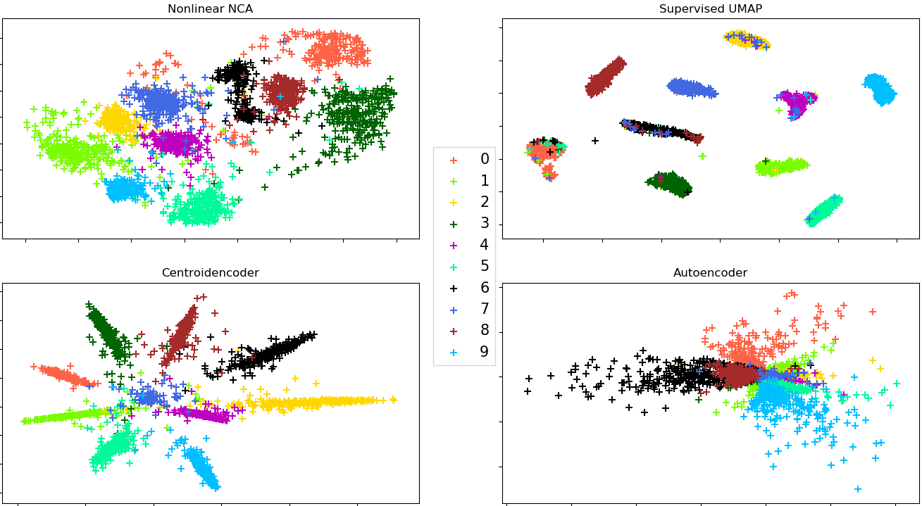
Figure 5: Two dimensional plot of 3000 USPS test digits by different dimensionality reduction methods.

In Figure 5, we show the two-dimensional visualization of 3,000 test samples using nonlinear NCA, supervised UMAP, centroid-encoder, and autoencoder. Like MNIST, the neighborhoods of CE and the other methods share many similarities. Digits 4, 9, and 7 are still neighbors in all the techniques but now sit more centrally. Digits 8 and 6 are now consistently neighbors across all methods. The within-class scatter of each digit is again the highest for autoencoder since it is unsupervised. Nonlinear NCA also has considerable variance across all the digit classes. Supervised UMAP has tighter clumping of the classes – apparently an integral feature of SUMAP as well as UMAP. However, supervised UMAP has some misplaced digits compared to CE, which is evident from the error rate in Table 3. These observations are consistent with MNIST visualizations. SUMAP emphasizes the importance of local structure over the global structure of the data. In contrast to CE, Autoencoder doesn’t provide any meaningful information about the neighborhood structure.

6.3.3 Letter, Landsat and Phoneme Data Sets

Here we compare centroid-encoder with another suite of supervised methods including, SNeRV, PE, S-Isomap, MUHSIC, MRE, and NCA. Table 5 shows the results on three benchmarking data sets, including UCI Letter, Landsat, and Phoneme dataset. On Landsat data, we include UMAP and SUMAP for additional comparison. CE produces the smallest prediction error on Landsat and Phoneme data sets and is ranked second on the Letter data set. On Landsat dataset, the top three models are CE, SUMAP and UMAP. On the Phoneme dataset, the centroid-encoder outperforms the second-best model, which is S-Isomap, by a margin of $1.9\%$. Notably, the variance of errors of centroid-encoder ($1.33$) is better than the S-Isomap ($5.74$). On the Letter dataset, the centroid-encoder achieves the error rate of $23.82\%$, which is the second-best model after SNeRV ($\lambda=0.1$), although the variance of the result of centroid-encoder is better than SNeRV by a margin of $1.47$. It’s also noteworthy that the variance of errors for centroid-encoder is the lowest in every case.

Method	Dataset
	Letter	Landsat	Phoneme
CE	$23.82\pm 3.13$	$\textbf{8.97}\pm\textbf{2.55}$	$\textbf{7.52}\pm\textbf{1.33}$
SUMAP	NA	$9.68\pm 3.12$	NA
UMAP	NA	$11.89\pm 2.83$	NA
SNeRV $\lambda=0.1$	$\textbf{22.96}\pm\textbf{4.6}$	$14.34\pm 7.38$	$9.43\pm 7.79$
SNeRV $\lambda=0.3$	$24.59\pm 4.6$	$13.93\pm 6.97$	$9.02\pm 7.38$
PE	$31.15\pm 4.92$	$14.75\pm 8.20$	$9.84\pm 6.15$
S-Isomap	$31.97\pm 7.38$	$15.16\pm 9.02$	$8.61\pm 5.74$
NCA	$62.30\pm 5.74$	$15.57\pm 7.38$	$20.49\pm 5.73$
MUHSIC	$79.51\pm 4.92$	$15.37\pm 4.10$	$14.75\pm 4.1$
MRE	$90.98\pm 7.38$	$53.28\pm 34.2$	$45.08\pm 18.03$

Table 5: Classification error (%) of $k$-NN ($k$=5) on the 2D embedded data by different supervised embedding methods on Letter, Landsat and Phoneme data. Average misclassifications over ten-fold cross-validation are shown along with standard deviation. Results of methods other than centroid-encoder, UMAP and SUMAP are reported from [34]. NA means result is not available.

The visualization of the two-dimensional embedding using centroid-encoder on Landsat is shown in Figure 6. We might conclude that the water content in the samples is causing scatter in the 2D plots and decreases as we proceed counter-clockwise. The test samples encode essentially the same structure. In Figure 7, we show the visualization using SUMAP. We see tighter clusters, but there is no difference between the damp and non-damp soil types. The neighborhood relationships, demonstrated by Laplacian Eigemaps, also show this transition by dampness consistent with CE. Damp and very damp soils are, however, not neighbors using SUMAP, making the visualization less informative.

(a) Two-dimensional plot of Landsat training samples.

(b) Two-dimensional plot of Landsat test samples.

Figure 6: Voronoi cells of low-dimensional Landsat data using a $16\rightarrow[250,150,2,150,250]\rightarrow 16$ centroid-encoder. Voronoi regions for each soil type are formed from the training set.

(a) Two-dimensional plot of Landsat training samples.

(b) Two-dimensional plot of Landsat test samples.

Figure 7: Voronoi cells of low-dimensional Landsat data using Supervised UMAP. Voronoi regions for each soil type are formed from the training set.

6.3.4 Iris, Sonar and USPS (revisited) Data Sets

In our last experiment, we compare supervised PCA and kernel supervised PCA to centroid-encoder. Table 6 contains the classification error using a 5-NN classifier, showing that centroid-encoder outperforms SPCA and KSPCA by considerable margins by this objective measure.

In the top row of Figure 8, we present the two-dimensional visualization of Iris test data. Among the three methods, centroid-encoder and KSPCA produce better separation compared to SPCA. SPCA can’t separate the Iris plants Versicolor and Virginica in 2D space. The dispersion of the three Iris categories is relatively higher in KSPCA and SPCA compared to centroid-encoder. Surprisingly in KSPCA, three classes are mapped on three separate lines.

The two-dimensional visualization of Sonar test samples is shown in the middle row of Figure 8. None of the methods can completely separate the two classes. The embedding of KSPCA is slightly better than SPCA, which doesn’t separate the data at all. In centroid-encoder, the two classes are grouped relatively far away from each other. Most of the rock samples are mapped at the bottom-left of the plot, whereas the mine samples are projected at the top-right corner.

The visualization of USPS test data is shown at the bottom of Figure 8. Both SPCA and KSPCA are unable to separate the ten classes, although KSPCA separates digit 0s from the rest of the samples. In contrast, the centroid-encoder puts the ten digit-classes in 2-D space without much overlap. Qualitatively, the embedding of centroid-encoder is better than the other two.

Method	Dataset
	IRIS	Sonar	USPS
Centroidencoder	$\textbf{3.29}\pm\textbf{2.10}$	$\textbf{14.24}\pm\textbf{2.99}$	$\textbf{12.16}\pm\textbf{2.01}$
KSPCA	$5.16\pm 4.56$	$21.06\pm 5.38$	$51.63\pm 2.11$
SPCA	$66.67\pm 0.00$	$49.06\pm 5.04$	$64.95\pm 1.94$

Table 6: $k$-NN ($k=5$) error (%) on the 2D embedded data by different supervised embedding methods on Iris, Sonar and USPS data. Note that given the limitations of KSPCA we have restricted the USPS data set to have 1000 total samples.

(a) KSPCA

(b) SPCA

(c) Centroid-encoder

(d) KSPCA

(e) SPCA

(f) Centroid-encoder

(g) KSPCA

(h) SPCA

(i) Centroid-encoder

Figure 8: Visualization of Iris (top row), Sonar (middle row) and USPS (bottom row) data using different dimensionality reduction techniques.

7 Discussion and Analysis of Results

The experimental results in Section 6.3 establish that centroid-encoder performs competitively, i.e., it is the best, or near the best, on a diverse set of data sets. The algorithms that produce similar classification rates require the computation of distance matrices and are hence more expensive than centroid-encoders. Here we analyze the CE algorithm in more detail to discover why this improved performance is perhaps not surprising. This has to do, at least in part, with the fact that centroid-encoder, implementing a nonlinear mapping, is actually able to capture more variance than PCA, and this is particularly important in lower dimensions.

7.1 Variance Plot to Explain the Complexity of Data

PCA captures the maximum variance over the class of orthogonal transformations [7]. The total variance captured as a function of the number of dimensions is a measure of the complexity of a data set. We can use variance to establish, e.g., that the digits 0 and 1 are less complex than the digits 4 and 9. To this end, we use two subsets from the MNIST training set: the first one contains all the digits 0 and 1, and the second one has all the digits 4 and 9. Next, we compute the total variance captured as a function of dimension; see Figure 9. Clearly, the variance is more spread out across the dimensions for the digits 4/9. In Figure 10, we show the visualization of these two subsets using PCA. We see that the 0/1 samples in subset1 are well separated in two-dimensional space, whereas the data in subset2 are clumped together. This lies in the fact that in low dimension (2D) PCA captures more variance from subset1 (around 41%) as compared to subset2 (about 22%). We can say that subset2 is more complex than subset1.

Figure 9: Variance plot using two different subsets (subset1: all the digits 0 and 1, subset2: all the digits 4 and 9) of MNIST data. Left: comparison of variance plot of the two subsets using the first 100 dimensions. Right: a blowup of the plot on the left showing the % of variance captured in low dimensions.

(a) Subset 1: digit 0 and 1

(b) Subset 2: digit 4 and 9

Figure 10: Two dimensional embedding using PCA for subset 1 and subset 2.

7.2 Centroid-encoder and Variance

In this section, we demonstrate how centroid-encoder maps a higher fraction of the variance of the data to lower dimensions. Again, consider the subset of digits 4 and 9 from the experiment above. We use all the digits 4 and 9 from the MNIST test set as a validation set. We trained a centroid-encoder with the architecture $784\rightarrow[784]\rightarrow 784$ where we used hyperbolic tangent (‘tanh’) as the activation function. We keep the number of nodes the same in all the three layers. After the training, we pass the training and test samples through the network and capture the hidden activation which we call CE-transformed data. We show the variance plot and the two-dimensional embedding by PCA on the CE-transformed data. Figure 11 compares the variance plot between the original data and the CE-transformed data. In the original data, only 22% of the total variance is captured, whereas about 89% of the total variance is captured in CE-transformed data. It appears that the nonlinear transformation of centroid-encoder puts the original high dimensional data in a relatively low dimensional space. Visualization using PCA of CE-transformed data (both training and test) is shown in Figure 12. This time, PCA separates the classes in two-dimensional space. Comparing Figure 12 with Figure 10(b), it appears that the transformation by centroid-encoder is helpful for low dimensional visualizations.

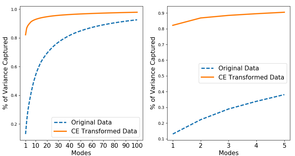
Figure 11: Variance plots for the 4/9 digit data. Left: comparison of variance plot of the original data and CE transformed data using the first 100 dimensions. Right: a blowup of the plot on the left showing the % of variance captured in low dimensions.

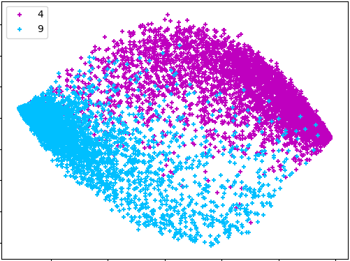
(a) Digits 4 and 9 from training set.

(b) Digits 4 and 9 from test set.

Figure 12: Two dimensional embedding using PCA on the CE-transformed data.

7.3 Computational Complexity and Scalability

The computational complexity of the centroid-encoder is effectively the same as the autoencoder. The advantage of centroid-encoder over many other data visualization techniques is that it is not necessary to compute pairwise distances. If everything else is fixed, we can view centroid-encoder as scaling linearly with the number of data points. Techniques that require distance matrices scale quadratically with the number of data points and can be prohibitively slow as the data set size increases. Methods based on distance matrices include NNCA, dt-NCA, dG-NCA, dt-MCML, and dG-MCML, as well as the spectral methods including MDS, UMAP, Laplacian Eigenmaps, Isomap and their supervised counterparts. The only overhead of centroid-encoder is the calculation of centroids of each class, but this is also linear with the number of classes.

8 Conclusion

In this paper, we presented the centroid-encoder for the task of data visualization when class labels are available. We compared CE to state-of-the-art techniques and showed advantages empirically over other methods. Our examples illustrate that CE captures the topological structure, i.e., neighborhoods of the data, comparable to methods, but with lower cost and generally better prediction error. These experiments include comparisons to the unsupervised Laplacian eigenmaps, UMAP, pt-SNE, autoencoders; the supervised UMAP, SPCA, KSPCA as well as the MCML and NCA class of algorithms. The algorithms that have the most similar prediction errors when compared to CE require the computation of distances between all pairs of points. We demonstrated that the 2D embedding of centroid-encoder produces competitive, if not optimal, prediction errors. We also showed empirically that the model globally captures high statistical variance relative to optimal linear transformations, i.e., more than PCA.

In addition to capturing the global topological structure of the data in low-dimensions, CE exploits data labels to minimize the within-class variance. This improves the localization of the mapping such that points are mapped more faithfully to their Voronoi regions in low-dimensions. CE also provides a mapping model that can be applied to new data without any retraining being necessary. This is in contrast to the spectral methods described here that require the entire training and testing set for computing the embedding eigenvectors.

In the future, we plan to extend the model in unsupervised and semi-supervised learning.

9 Acknowledgement

The authors thank Shannon Stiverson and Eric Kehoe to review the article thoroughly and giving us their feedback to make the material better. We also thank Manuchehr Aminian to make sure that the code in GitHub is working correctly.

References

- [1] Karl Pearson. On lines and planes of closest fit to systems of points in space. Phil. Mag. S., 2(11):559–572, 1901.
- [2] H. Hotelling. Analysis of a complex of statistical variables into principal components. Journal of Educational Psychology, September, 1933.
- [3] Ian T Jolliffe and Jorge Cadima. Principal component analysis: a review and recent developments. Philosophical Transactions of the Royal Society A: Mathematical, Physical and Engineering Sciences, 374(2065):20150202, 2016.
- [4] Mark A. Kramer. Nonlinear principal component analysis using autoassociative neural networks. AIChE J., 37(2):233–243, 1991.
- [5] Mark A. Kramer. Autoassociative neural networks. Comput. Chem. Engng., 16(4):313–328, 1992.
- [6] E. Oja. Data compression, feature extraction, and autoassociation in feedforward neural networks. In T. Kohonen, K. Mäkisara., O. Simula, and J. Kangas, editors, Artificial Neural Networks, pages 737–745, NY, 1991. Elsevier Science.
- [7] M. Kirby. Geometric Data Analysis: An Empirical Approach to Dimensionality Reduction and the Study of Patterns. Wiley, 2001.
- [8] D.S. Broomhead and M. Kirby. A new approach for dimensionality reduction: Theory and algorithms. SIAM J. of Applied Mathematics, 60(6):2114–2142, 2000.
- [9] D.S. Broomhead and M. Kirby. The Whitney reduction network: a method for computing autoassociative graphs. Neural Computation, 13:2595–2616, 2001.
- [10] Geoffrey E Hinton and Ruslan R Salakhutdinov. Reducing the dimensionality of data with neural networks. science, 313(5786):504–507, 2006.
- [11] Geoffrey E. Hinton, Simon Osindero, and Yee-Whye Teh. A fast learning algorithm for deep belief nets. Neural Comput., 18(7):1527–1554, July 2006.
- [12] I.T. Jolliffe. Principal Component Analysis. Springer, New York, 1986.
- [13] S. Watanabe. Karhunen–Loève expansion and factor analysis. In Trans. 4th. Prague Conf. on Inf. Theory, Statist. Decision Functions, and Random Proc., pages 635–660, Prague, 1965.
- [14] T. Kohonen. Self-organized formation of topologically correct feature maps. Biol. Cybern., 43:59, 1982.
- [15] W. S. Torgerson. Multidimensional scaling: I. theory and method. Psychometrika, 17:401–419, 1952.
- [16] Joshua B. Tenenbaum, Vin de Silva, and John C. Langford. A global geometric framework for nonlinear dimensionality reduction. Science, 290(5500):2319–2323, 2000.
- [17] Mikhail Belkin and Partha Niyogi. Laplacian eigenmaps for dimensionality reduction and data representation. Neural Comput., 15(6):1373–1396, June 2003.
- [18] Sam T. Roweis and Lawrence K. Saul. Nonlinear dimensionality reduction by locally linear embedding. SCIENCE, 290:2323–2326, 2000.
- [19] Geoffrey E Hinton and Sam T. Roweis. Stochastic neighbor embedding. In S. Becker, S. Thrun, and K. Obermayer, editors, Advances in Neural Information Processing Systems 15, pages 857–864. MIT Press, 2003.
- [20] Killan Q. Weinberger and Lawrence K. Saul. An introduction to nonlinear dimensionality reduction by maximum variance unfolding. In Proceedings of the 21st National Conference on Artificial Intelligence - Volume 2, AAAI’06, pages 1683–1686. AAAI Press, 2006.
- [21] Laurens van der Maaten and Geoffrey Hinton. Visualizing data using t-SNE. Journal of Machine Learning Research, 9:2579–2605, 2008.
- [22] Leland McInnes, John Healy, and James Melville. Umap: Uniform manifold approximation and projection for dimension reduction. arXiv preprint arXiv:1802.03426, 2018.
- [23] Vin De Silva and Joshua B Tenenbaum. Sparse multidimensional scaling using landmark points. Technical report, Technical report, Stanford University, 2004.
- [24] R. A. Fisher. The use of multiple measurements in taxonomic problems. Annals of Eugenics, 7(7):179–188, 1936.
- [25] R. O. Duda and P. E. Hart. Pattern Classification and Scene Analysis. John Willey & Sons, New York, 1973.
- [26] Eric Bair, Trevor Hastie, Debashis Paul, and Robert Tibshirani. Prediction by supervised principal components. Journal of the American Statistical Association, 101(473):119–137, 2006.
- [27] Elnaz Barshan, Ali Ghodsi, Zohreh Azimifar, and Mansoor Zolghadri Jahromi. Supervised principal component analysis: Visualization, classification and regression on subspaces and submanifolds. Pattern Recogn., 44(7):1357–1371, July 2011.
- [28] Le Song, Alexander J. Smola, Karsten M. Borgwardt, and Arthur Gretton. Colored maximum variance unfolding. In NIPS, 2007.
- [29] Jacob Goldberger, Sam Roweis, Geoff Hinton, and Ruslan Salakhutdinov. Neighbourhood components analysis. In Proceedings of the 17th International Conference on Neural Information Processing Systems, NIPS’04, pages 513–520, Cambridge, MA, USA, 2004. MIT Press.
- [30] Tomoharu Iwata, Kazumi Saito, Naonori Ueda, Sean Stromsten, Thomas L. Griffiths, and Joshua B. Tenenbaum. Parametric embedding for class visualization. Neural Comput., 19(9):2536–2556, September 2007.
- [31] Ruslan Salakhutdinov and Geoff Hinton. Learning a nonlinear embedding by preserving class neighbourhood structure. In Artificial Intelligence and Statistics, pages 412–419, 2007.
- [32] Amir Globerson and Sam T Roweis. Metric learning by collapsing classes. In Advances in neural information processing systems, pages 451–458, 2006.
- [33] Martin R Min, Laurens Maaten, Zineng Yuan, Anthony J Bonner, and Zhaolei Zhang. Deep supervised t-distributed embedding. In Proceedings of the 27th International Conference on Machine Learning (ICML-10), pages 791–798, 2010.
- [34] Jarkko Venna, Jaakko Peltonen, Kristian Nybo, Helena Aidos, and Samuel Kaski. Information retrieval perspective to nonlinear dimensionality reduction for data visualization. J. Mach. Learn. Res., 11:451–490, March 2010.
- [35] Jian Cheng, Can Cheng, and Yi-nan Guo. Supervised isomap based on pairwise constraints. In Proceedings of the 19th International Conference on Neural Information Processing - Volume Part I, ICONIP’12, pages 447–454, Berlin, Heidelberg, 2012. Springer-Verlag.
- [36] Shi-qing Zhang. Enhanced supervised locally linear embedding. Pattern Recogn. Lett., 30(13):1208–1218, October 2009.
- [37] B. Raducanu and F. Dornaika. A supervised non-linear dimensionality reduction approach for manifold learning. Pattern Recogn., 45(6):2432–2444, June 2012.
- [38] Andre Stuhlsatz, Jens Lippel, and Thomas Zielke. Feature extraction with deep neural networks by a generalized discriminant analysis. IEEE transactions on neural networks and learning systems, 23(4):596–608, 2012.
- [39] Martin Renqiang Min, Hongyu Guo, and Dongjin Song. Exemplar-centered supervised shallow parametric data embedding. arXiv preprint arXiv:1702.06602, 2017.
- [40] Fabian Pedregosa, Gaël Varoquaux, Alexandre Gramfort, Vincent Michel, Bertrand Thirion, Olivier Grisel, Mathieu Blondel, Peter Prettenhofer, Ron Weiss, Vincent Dubourg, Jake Vanderplas, Alexandre Passos, David Cournapeau, Matthieu Brucher, Matthieu Perrot, and Édouard Duchesnay. Scikit-learn: Machine learning in python. J. Mach. Learn. Res., 12:2825–2830, November 2011.
- [41] Tomojit Ghosh, Xiaofeng Ma, and Michael Kirby. New tools for the visualization of biological pathways. Methods, 132:26 – 33, 2018. Comparison and Visualization Methods for High-Dimensional Biological Data.
- [42] Mark A. Kramer. Nonlinear principal component analysis using autoassociative neural networks. AIChE Journal, 37(2):233–243, 1991.
- [43] Yoshua Bengio, Pascal Lamblin, Dan Popovici, and Hugo Larochelle. Greedy layer-wise training of deep networks. In Proceedings of the 19th International Conference on Neural Information Processing Systems, NIPS’06, pages 153–160, Cambridge, MA, USA, 2006. MIT Press.
- [44] David E Rumelhart, Geoffrey E Hinton, and Ronald J Williams. Learning internal representations by error propagation. Technical report, DTIC Document, 1985.
- [45] P.J. Werbos. Beyond Regression: New Tools for Prediction and Analysis in the Behavioral Sciences. PhD dissertation, Harvard University, August 1974.
- [46] P. Baldi and K. Hornik. Neural networks and principal component analysis: Learning from examples without local minima. Neural Netw., 2(1):53–58, January 1989.
- [47] M. Kirby and R. Miranda. Empirical dynamical system reduction I: Global nonlinear transformations. In K. Coughlin, editor, Semi-analytic Methods for the Navier–Stokes Equations (Montreal, 1995), volume 20 of CRM Proc. Lecture Notes, pages 41–64, Providence, RI, 1999. Amer. Math. Soc.
- [48] M. Kirby and R. Miranda. Circular nodes in neural networks. Neural Computation, 8(2):390–402, 1996.
- [49] D. Hundley, M. Kirby, and R. Miranda. Spherical nodes in neural networks with applications. In S.H. Dagli, B.R. Fernandez, J. Ghosh, and R.T. Soundar Kumara, editors, Intelligent Engineering Through Artificial Neural Networks, volume 5, pages 27–32, New York, 1995. The American Society of Mechanical Engineers.
- [50] K. Hornik, M. Stinchcombe, and H. White. Multilayer feedforward networks are universal approximators. Neural Netw., 2(5):359–366, July 1989.
- [51] G. Cybenko. Approximation by superpositions of a sigmoidal function. Mathematics of Control, Signals and Systems, 2(4):303–314, Dec 1989.
- [52] Yoshua Bengio, Pascal Lamblin, Dan Popovici, and Hugo Larochelle. Greedy layer-wise training of deep networks. In B. Schölkopf, J. C. Platt, and T. Hoffman, editors, Advances in Neural Information Processing Systems 19, pages 153–160. MIT Press, 2007.
- [53] Marc’ Aurelio Ranzato, Y-Lan Boureau, and Yann LeCun. Sparse feature learning for deep belief networks. In Proceedings of the 20th International Conference on Neural Information Processing Systems, NIPS’07, pages 1185–1192, USA, 2007. Curran Associates Inc.
- [54] Honglak Lee, Chaitanya Ekanadham, and Andrew Y. Ng. Sparse deep belief net model for visual area v2. In J. C. Platt, D. Koller, Y. Singer, and S. T. Roweis, editors, Advances in Neural Information Processing Systems 20, pages 873–880. Curran Associates, Inc., 2008.
- [55] Pascal Vincent, Hugo Larochelle, Isabelle Lajoie, Yoshua Bengio, and Pierre-Antoine Manzagol. Stacked denoising autoencoders: Learning useful representations in a deep network with a local denoising criterion. J. Mach. Learn. Res., 11:3371–3408, December 2010.
- [56] Jonathan Masci, Ueli Meier, Dan Cireşan, and Jürgen Schmidhuber. Stacked convolutional auto-encoders for hierarchical feature extraction. In Proceedings of the 21th International Conference on Artificial Neural Networks - Volume Part I, ICANN’11, pages 52–59, Berlin, Heidelberg, 2011. Springer-Verlag.
- [57] Xifeng Guo, Xinwang Liu, En Zhu, and Jianping Yin. Deep clustering with convolutional autoencoders. In Derong Liu, Shengli Xie, Yuanqing Li, Dongbin Zhao, and El-Sayed M. El-Alfy, editors, Neural Information Processing, pages 373–382, Cham, 2017. Springer International Publishing.
- [58] Eli David and Nathan S. Netanyahu. Deeppainter: Painter classification using deep convolutional autoencoders. CoRR, abs/1711.08763, 2017.
- [59] Ian Goodfellow, Yoshua Bengio, and Aaron Courville. Deep Learning. MIT Press, 2016. http://www.deeplearningbook.org.
- [60] Y. Linde, A. Buzo, and R. Gray. An algorithm for vector quantization design. IEEE transactions on Communications, 28(1):84–95, January 1980.
- [61] Laurens van der Maaten. Learning a parametric embedding by preserving local structure. In AISTATS, volume 5 of JMLR Proceedings, pages 384–391. JMLR.org, 2009.
- [62] Roland Memisevic and Geoffrey Hinton. Multiple relational embedding. In Proceedings of the 17th International Conference on Neural Information Processing Systems, NIPS’04, pages 913–920, Cambridge, MA, USA, 2004. MIT Press.
- [63] Dheeru Dua and Casey Graff. UCI machine learning repository, 2017.
- [64] Diederik P. Kingma and Jimmy Ba. Adam: A method for stochastic optimization. CoRR, abs/1412.6980, 2014.