Generation, manipulation and detection of snake state trajectories of a neutral atom in a ring-cavity

Abstract

We propose a set-up which can be used to create and detect the atomic counterpart of snake state trajectories observed in electronic systems where either sign of the charge-carrier changes or the magnetic field changes direction. In this work, we use a laser-induced synthetic gauge field that depends on the cavity photon numbers to generate such trajectories. We analyse the motion of a single atom in the presence of such a gauge field while including the back-action of the cavity fields. We demonstrate that the output cavity field provides a non-destructive way of observing the real-time atomic dynamics inside the ring cavity. We also show that we can tune the system parameters to modify the properties of the snake state and even amplify the effect of cavity feedback to destroy the snake-like trajectories.

I Introduction

Figure 1: (color online) (a) Schematic for a single two-level atom trapped inside a ring cavity. The cavities are pumped on-axis with strengths $\eta_{1}$ and $\eta_{2}$. The cavity photons interact with the atom and give rise to the atom-photon coupling $g(y)$. $\kappa$ is the cavity decay rate. (b) Vector potential $A_{x}(y)$ (in units of $B_{0}l_{B}$) $(blue$ curve) as a function of $y/w_{0}$ and magnetic field $B_{z}(y)$ (in units of $B_{0}=\frac{\hbar k}{w_{0}}$) $(orange$ curve) as a function of $y/w_{0}$ for fixed $n_{1}$=342 and $n_{2}$=8. The vector potential is calculated in units of $B_{0}l_{B}$ which has dimensions of recoil momentum, $\hbar k$. The magnetic field flips direction as $y$ changes sign. As the difference between $n_{1}$ and $n_{2}$ changes sign, the resulting magnetic field also flips the direction from $-\hat{z}$ to $+\hat{z}$. (c) Atomic snake-like trajectories - $y_{a}(t)/w_{0}$ as a function of $x_{a}(t)\lambda_{p}$, including the cavity back-action. (d) $x-$ position ($blue$ curve) of atom - $x_{a}/\lambda_{p}$ ($left$ $y-$ axis) as a function of $t$, and $y-$ position ($red$ curve) of the atom - $y_{a}/w_{0}$ ($right$ $y-$ axis) as a function of $t$ with cavity backaction. The dotted curves in (c) and (d) show the atomic trajectory, $x-$ position and the $y-$ position without the backaction for fixed $n_{1}$ and $n_{2}$ used in (b).

Ultracold atomic gases in tailored optical potentials can quantum simulate the key electronic properties of dirty solid state systems in extremely well-controlled and tunable environments, magnified by several orders of magnitude compared to original solid materials [1, 3, 2, 4]. The advancement of quantum gas microscopes [5] and optical tweezers arrays [6] has further solidified the application of these systems for understanding quantum many-body systems and their possible application to quantum technology. In such simulators, the analogue of the electromagnetic fields that act on the charge carriers in solid state devices are the laser-induced synthetic gauge fields that can be realised by coupling different internal states of the charge-neutral atoms [7, 8, 9, 10, 11, 12, 13, 14, 15, 16] to generate various exciting states of matter. Here, we study one such example, which is called snake states - special one-dimensional current-carrying states that occur in two-dimensional electron gas (2DEG) due to magnetic field gradient, and exist at the boundary where the applied transverse magnetic field changes sign ($\boldsymbol{B}=0$). Snake states were first studied theoretically in a two-dimensional electron gas (2DEG) by Müller [17] and their first experimental confirmation was carried out in a 2DEG realised in GaAs-AlGaAs heterostructure by K. von Klitzing’s group [18] and subsequently in graphene [19, 20]. These developments were theoretically analysed in great detail and have been reviewed in a large number of works [21, 22, 23, 24, 25, 26, 27, 28]. From a cold-atom perspective, such states can be used for a topologically protected long-distance transport which is crucial for atomtronics [29, 30, 31] as well as quantum information processing [32].

In this work, we show that snake states can be realized, manipulated and detected in a nearly non-destructive way by coupling a two-level atom to two counter-propagating and orthogonally polarized running wave modes of a high-finesse ring cavity. Using a dressed state approach, we derive semi-classical equations of motion of the system and show that a non-uniform synthetic magnetic field that changes its sign about a point of symmetry can be generated. The structure of this magnetic field is governed by the transverse mode structure of the cavity modes and the corresponding amplitude is proportional to the difference in the photon number in the two cavity modes. We show that a snake state trajectory can be generated by pumping just one of the two cavity modes with minimal effect of the cavity backaction [33]. Furthermore, the amplitude and phase of the light scattered by the atom into the other cavity mode can be used to reconstruct the snake state trajectory in real time and over a length scale which is order of magnitude longer than their solid state counterpart. We further demonstrate that by tuning the strength of atom-cavity coupling, we can tune the relative photon number in the two cavity modes. This allows us to not only reverse the direction of snake states, but also enhance the role of cavity backaction leading to the destruction of snake state trajectories. Coupling quantum gases with single and multi-mode high-finesse optical cavities has already simulated and experimentally tested a number of highly interesting phenomena such as Dicke superradiance [34], continuous supersolid [35], quantum phonons of quantum optical lattices [36], dynamical synthetic gauge field to observe analogue of Meissner effect in superconductors [37] ( for a recent review and a more complete list see [38, 39]). Our proposed set-up can lead to new experiments and applications in the field of atomtronics.

Accordingly the rest of the paper is organised as follows. In Section II, we describe the considered ring cavity system and the resulting system Hamiltonian. We derive the Schrödinger equation for the atomic wavefunction and obtain the equation for the probability amplitude for the atom to be in the lowest energy dressed state. Due to the adiabatic following of the lowest energy dressed state, we get a vector potential which gives rise to a non-uniform magnetic field. In Section III, we obtain the semiclassical snake-like trajectories of the atom moving in the presence of such a non-uniform magnetic field including the back-action of the cavity fields on the atomic motion. We also provide an analysis of the output cavity fields which carry information about the presence of the snake states inside the cavity in Section IV. We then show how the snake states can be manipulated by varying the system parameters in Section V and discuss the effect of cavity feedback on these states in Section VI. We provide the conclusions in Section VII.

II System Hamiltonian

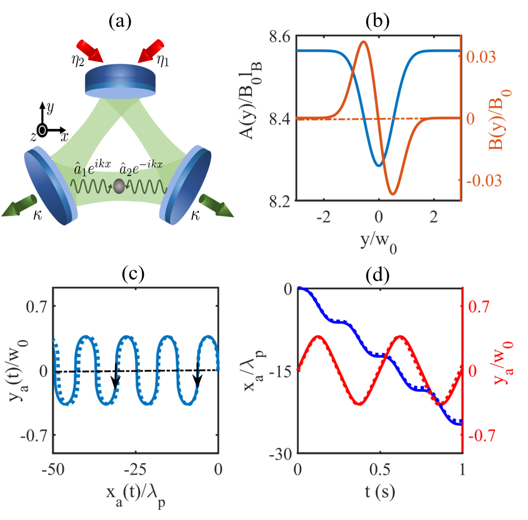
We consider a single two-level atom with internal states $|g\rangle$ and $|e\rangle$ coupled to two counter-propagating running wave modes of a ring cavity as shown in Fig. 1(a). The two cavity modes are pumped on-axis with pump strengths $\eta_{1}$ and $\eta_{2}$. The total Hamiltonian describing the coupled atom-cavity system in the rotating frame of the pump field space [40] can be written as (see Appendix A for details)-

$$\hat{H}_{RF} = \hat{H}_{0}+\hat{H}_{I}$$ (1)

where

$$\hat{H}_{0} = \frac{\hat{P}^{2}}{2m_{a}}\hat{\mathbb{I}}$$

$$\hat{H}_{I} = -\frac{\hbar\Delta_{a}\hat{\sigma}_{z}}{2}-\hbar\Delta_{c}\left(\hat{a}^{{\dagger}}_{1}\hat{a}_{1}+\hat{a}^{{\dagger}}_{2}\hat{a}_{2}\right)$$

$$+ \hbar\eta_{1}\left(\hat{a}_{1}+\hat{a}^{{\dagger}}_{1}\right)+\hbar\eta_{2}\left(\hat{a}_{2}+\hat{a}^{{\dagger}}_{2}\right)$$

$$+ \hbar\left(g_{1}(y)\hat{\sigma}^{+}\hat{a}_{1}e^{ikx}+g_{2}(y)\hat{\sigma}^{+}\hat{a}_{2}e^{-ikx}\right.$$

$$+ \left.g_{1}(y)\hat{\sigma}^{-}\hat{a}^{{\dagger}}_{1}e^{-ikx}+g_{2}(y)\hat{\sigma}^{-}\hat{a}^{{\dagger}}_{2}e^{ikx}\right)$$

$\hat{H}_{0}$ is the kinetic energy of the atom. $\hat{\mathbb{I}}=|g\rangle\langle g|+|e\rangle\langle e|$ is the identity operator in the internal two-dimensional Hilbert space of the atom, $m_{a}$ is the atom mass, and $\vec{r}$ and $\vec{P}$ are the atomic centre-of-mass co-ordinate and momentum respectively. $\omega_{a}$ is the atomic resonance frequency, $\omega_{p}$ is the pump frequency, $\omega_{c}$ is the cavity resonance frequency, $\Delta_{a}=\omega_{p}-\omega_{a}$ is the atom-pump detuning and $\Delta_{c}=\omega_{p}-\omega_{c}$ is the cavity-pump detuning. $\hat{\sigma}_{z}=|e\rangle\langle e|-|g\rangle\langle g|$ is the Pauli matrix. $\hat{\sigma}^{+}$ and $\hat{\sigma}^{-}$ are the atomic raising and lowering operators. $g_{1,2}(y)=g_{10,20}e^{-y^{2}/w^{2}_{0}}$ is the atom-photon coupling, with $w_{0}$ being the waist of the the two cavity modes and $g_{10,20}=\frac{-\vec{d}\cdot\hat{e}_{y,z}}{\hbar}\sqrt{\frac{\hbar\omega_{c}}{2\epsilon_{0}V}}$ with $|g_{10}|=|g_{20}|=g_{0}$. $\hat{a}_{1}$ and $\hat{a}_{2}$ are the annihilation operators for the two cavity modes with respective spatial mode profiles of the form $e^{ikx}e^{-y^{2}/w_{0}^{2}}$ and $e^{-ikx}e^{-y^{2}/w_{0}^{2}}$, with $k=2\pi/\lambda_{p}$. Following a mean-field approach, we assume that the cavity fields can be described by a coherent state of the form $|\alpha_{1},\alpha_{2}\rangle=|\alpha_{1}\rangle|\alpha_{2}\rangle$ with $\hat{a}_{1,2}|\alpha_{1,2}\rangle=\alpha_{1,2}|\alpha_{1,2}\rangle$ and $n_{1(2)}=|\alpha_{1(2)}|^{2}$ being the average photon number in the cavity mode 1(2). We assume that all the dynamics take place in the $x-y$ plane, so we have neglected the $z$-coordinate in different expressions.

Figure 2: color online: (a) Fourier transform for $y_{a}/w_{0}$ shows a peak at $\nu_{0}\approx 2$ Hz, (b) Photon numbers in cavity mode 2, $n_{2}$ $(blue$ curve) and phase of photons in mode 2, $\phi_{2}$ $(black$ curve) as a function of $t$. (c) Fourier transform of $n_{2}$ shows peaks at $2\nu_{0}$, $4\nu_{0}$, $6\nu_{0}$ and so on. (d) Fourier transform of $e^{i\phi_{2}}$ shows several peaks at various frequencies and overlaps with the Fourier transform of $e^{2ikx_{a}}$.

We diagonalise the interaction Hamiltonian $\hat{H}_{I}$ in the space spanned by the atom-photon bare-states, namely $|e,\alpha_{1},\alpha_{2}\rangle,$ and $|g,\alpha_{1},\alpha_{2}\rangle$, and obtain the eigenstates that are called dressed states $|D_{1,2}\rangle$, for the coupled atom-photon system, with eigen energies $E_{1,2}$, see Appendix B for details. Under adiabatic approximation, [7, 41, 42, 43, 44, 45, 46, 47, 48, 49, 50], we can limit the system dynamics in the eigenspace of the lowest energy dressed state $|D_{1}\rangle$, and obtain the following equation for the evolution of the corresponding wave function $\psi_{1}$ (see Appendix C) -

$$\boxed{i\hbar\frac{\partial}{\partial t}\psi_{1}(\vec{r},t)=H_{S}\psi_{1}(\vec{r},t)=\Big{[}\frac{1}{2m_{a}}\Big{\{}\left(\vec{p}-\vec{\textbf{A}}_{1,1}\right)^{2}+|\vec{\textbf{A}}_{2,1}|^{2}\Big{\}}+E_{1}\Big{]}\psi_{1}(\vec{r},t)}$$ (2)

Here, $\vec{\textbf{A}}_{1,1}$ acts as a synthetic vector potential while $\vec{\textbf{A}}_{2,1}$ contributes to the synthetic scalar potential term, given by $W=\frac{1}{2m_{a}}|\vec{\textbf{A}}_{2,1}|^{2}$. The last term of Eq.(2), $E_{1}$, acts as a deep trapping potential for the atomic centre-of-mass motion. In the next section, we will explain why the important dynamics of the system are governed only by the vector potential, $\vec{\textbf{A}}_{1,1}$. The scalar potential, the vector potential and the corresponding magnetic field obtained here depend on the photon number in the two cavity modes which dynamically depends on the position of the atom.

The full expression for the vector potential in Eq. (2) is given as -

$$\vec{\textbf{A}}_{1,1} = i\hbar\langle D_{1}|\vec{\nabla}|D_{1}\rangle=A_{x}(y)\hat{x}$$ (3)

$$= \frac{2\hbar kg_{0}^{2}(y)(n_{1}-n_{2})}{G(G+\Delta_{a})}\hat{x}$$

where $G=\sqrt{\Delta_{a}^{2}+4g_{0}^{2}(y)\left(n_{1}+n_{2}\right)}$. The corresponding magnetic field is -

$$\vec{B} = -\frac{\partial A_{x}}{\partial z}\hat{z}=B_{0}\frac{y}{w_{0}}\frac{\Delta_{a}}{G^{3}}4g_{0}^{2}(y)(n_{1}-n_{2})\hat{z}$$ (4)

where $B_{0}=\frac{\hbar k}{w_{0}}$ defines the unit of the synthetic magnetic field with dimension $[MT^{-1}]$ and the corresponding synthetic magnetic length is given by $l_{B}=\sqrt{\frac{\hbar}{B_{0}}}$. Here, we observe that both the vector potential and the magnetic field scale with the difference in the photon numbers in the two cavity modes, $n_{1}$ and $n_{2}$ and thus can be tuned via $\eta_{1,2}$, $\Delta_{c}$ and the value of $g_{0}$. The parameters considered in this work are - $m_{a}=1.4\times 10^{-25}$ kg, $\Delta_{c}=-5\kappa$, $g_{0}=2\pi\times 50$ MHz, $\kappa=2\pi\times 650$ kHz, $\lambda_{p}=780.25$ nm, $\Delta_{a}=-2\pi\times 4.9$ GHz , $w_{0}=10$ $\mu$m, $\eta_{1}=80\kappa$ and $\eta_{2}=0$. This gives us $l_{B}=1.1$ $\mu$m and $B_{0}=8.48\times 10^{-23}$ kg/s. Using the magnetic length, the natural velocity scale of the system is $v_{0}=\hbar/(m_{a}l_{B})=655$ $\mu$m/s. As $v_{0}<<\hbar k/m_{a}=5.9$ mm/s which justifies the adiabatic approximation that when the atom moves slowly enough, it remains in the state in which it started ($|D_{1}\rangle$ in our case).

In Fig. 1(b), we plot the vector potential and the magnetic field. The vector potential $A_{x}(y)$ has a symmetric Gaussian profile given by the cavity mode shape. The corresponding magnetic field $B_{z}$ scales linearly for $y<<w_{0}$ with a slope proportional to $n_{1}-n_{2}$ and thus can give rise to snake state trajectories. $B_{z}$ achieves its maximum magnitude at $|y|=0.5w_{0}$ and decays smoothly to $0$ for $|y|>0.5w_{0}$. In the subsequent sections, we shall discuss the dynamics of a single atom in the presence of such non-uniform magnetic fields using a semiclassical method. It may be pointed out that such inhomogeneous synthetic gauge field can be created using different methods [51, 52]. However, coupling to a ring-cavity allows for nearly non-destructive monitoring of the resultant dynamics as we show below.

Figure 3: color online: (a) Frequency variation as a function of initial velocity along the $y$-direction for fixed $v_{x}$. We have considered four points $(v_{1})$, $(v_{2})$, $(v_{3})$ and $(v_{4})$ of initial velocity and show the corresponding trajectories and photon numbers. The $v_{y}$ velocity at point $v_{2}$ has been considered in the preceding figures and the rest of the paper and therefore, its trajectories are not shown here. Snake state trajectories for $v_{y}=v_{1}$, $v_{3}$ and $v_{4}$ are shown in (b), (d) and (f) respectively. Similarly, photon number ($black$ curve) in mode 2 ($left$ $y$ axis) and $y_{a}/w_{0}$ ($purple$ curve) variation ($right$ $y-$ axis) as a function of time for $v_{y}=v_{1}$, $v_{3}$ and $v_{4}$ are shown in (c), (e) and (g) respectively. For parameters and explanation, refer text.

III Trajectories of a single atom and backaction of the cavity fields

We now obtain the following semi-classical equation of motion for the atom due to the adiabatic following of the lowest energy dressed state (see Appendix D for details) [53, 54] -

$$m_{a}\frac{d\vec{v}}{dt}=-\vec{\nabla}E_{1}-\vec{\nabla}W(\vec{r})+\vec{v}\times\vec{B}(\vec{r}).$$ (5)

We want to isolate the effect of the $B(y)$ term on the atomic trajectory, so we neglect the $E_{1}+W$ contribution. In a real multi-level atom, the effect of $E_{1}+W$ can be removed by proper choice of the pump wavelength. So, the two components of the equation of motion become

$$m_{a}\frac{d^{2}x}{dt^{2}} = B(y)\frac{dy}{dt}$$ (6a)

$$m_{a}\frac{d^{2}y}{dt^{2}} = -B(y)\frac{dx}{dt}$$ (6b)

The solution of the above equations gives us the values of $x(t)$ and $y(t)$. To find the magnetic field, we need to additionally evaluate the number of photons in the two cavity modes. As $\kappa>>\hbar k^{2}/2m_{a},\hbar/(2m_{a}l_{b}^{2})$, we assume that the cavity field is always in a steady state and adiabatically follows the atomic motion. We, thus obtain the following average values of the two cavity fields.

$$\alpha_{1,2} = \langle\hat{a}_{1,2}\rangle=\langle D_{1}|\hat{a}_{1,2}|D_{1}\rangle$$

$$= \frac{i\eta_{1,2}(i\bar{\Delta}_{c}-\bar{\kappa})+i\eta_{2,1}(iM+P)e^{\mp 2ikx_{a}(t)}}{(i\bar{\Delta}_{c}-\bar{\kappa})^{2}-(iM+P)^{2}}$$

where $U_{0}=\frac{\Delta_{a}g_{0}^{2}}{\Delta_{a}^{2}+4\Gamma^{2}}$, $U=U_{0}e^{-2y_{a}^{2}(t)/w_{0}^{2}}$, $\gamma=\frac{2\Gamma g_{0}^{2}}{\Delta_{a}^{2}+4\Gamma^{2}}$, $\gamma=\gamma_{0}e^{-2y_{a}^{2}(t)/w_{0}^{2}}$, $\bar{\Delta}_{c}=\Delta_{c}-U$, $\bar{\kappa}=\kappa+\gamma$, $M_{0}=\frac{\Delta_{a}g^{2}_{0}}{\Delta_{a}^{2}+4\Gamma^{2}}$, $M=M_{0}e^{-2y_{a}^{2}(t)/w_{0}^{2}}$, $P_{0}=\frac{2\Gamma g^{2}_{0}}{\Delta_{a}^{2}+4\Gamma^{2}}$ and $P=P_{0}e^{-2y_{a}^{2}(t)/w_{0}^{2}}$. To obtain the atomic trajectory in the $x-y$ plane, we solve Eq.(6a, 6b) simultaneously with Eq.(LABEL:alpha12). We take initial velocity $v_{x}=0$ and $v_{y}=0.06v_{0}$. We plot $y_{a}(t)$ as a function of $x_{a}(t)$ in Fig. 1(c) and realize that the particle follows the so-called snake-state trajectory. The origin of such a trajectory is the following: The atom experiences a magnetic field which reverses its direction around $y=0$ and thus for $v_{x}=0\neq v_{y}$, a finite particle current is generated along -$x-$direction [17, 55]. The radius of curvature for the particle trajectory is inversely proportional to the synthetic magnetic field $(r\propto\frac{1}{B(y)})$. Therefore, for large(small) magnitude of the magnetic field and thus large(small) $|y|$, the particle will trace a trajectory with a small(large) radius of curvature and this results in the peculiar shape of the trajectory in the $x-y$ plane.

We plot $x_{a}(t)$ and $y_{a}(t)$ as a function of $t$ in Fig. 1(d). The dotted curves in Fig. 1(c,d) show the atomic trajectories and the atom’s $x-$ and $y-$ positions without considering the backaction of the cavity fields. Along $x$, the particle always has a finite average speed with an additional nonlinear behavior. Along $y-$direction, the particle oscillates periodically around $y=0$. The dashed curves in Fig. 1(c,d) illustrate the particle trajectories when the number of photons in the two cavity modes is fixed to the time-averaged values as given by Eq.(LABEL:alpha12), see Fig. 2 for the full time evolution of the cavity fields. We observe that the cavity-feedback minimally affects the snake state trajectory of the particle. As we show in the next section, the output cavity fields provide a non-destructive means of monitoring such snake state trajectory of the particle inside the cavity.

IV Cavity-based detection of the snake-like trajectories

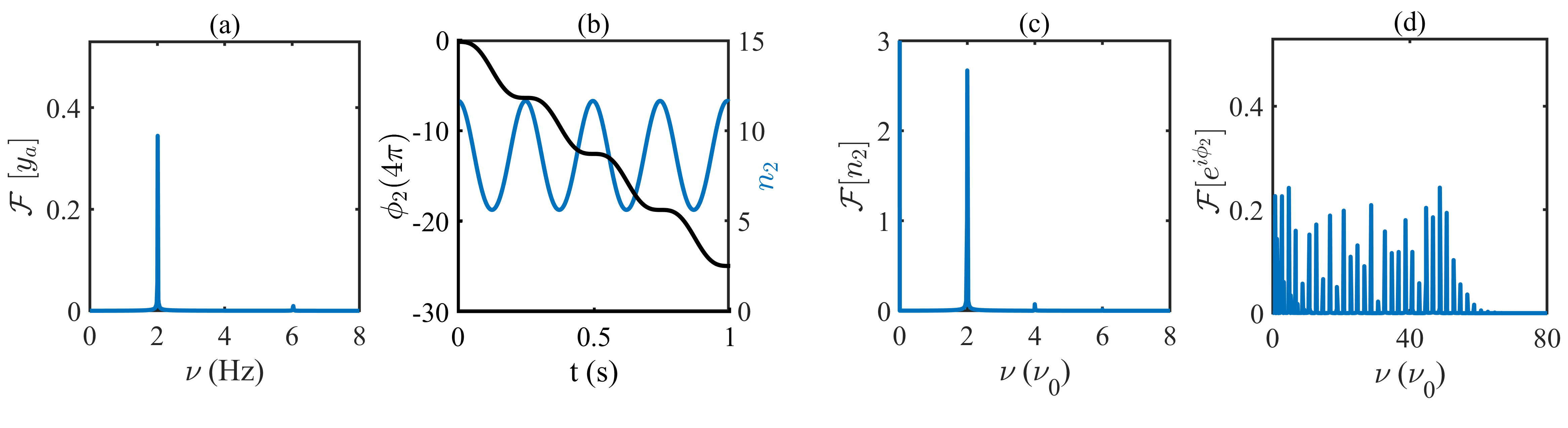
To probe the snake-state trajectory, we now look at the time evolution of the cavity field of mode 2, $\alpha_{2}=\sqrt{n_{2}}e^{i\phi_{2}}$. This is illustrated in Fig. 2(b). We realize that the time variation of phase $\phi_{2}$ and photon number $n_{2}$ is qualitatively similar to respectively the $x$ and $y$ variation of the atomic trajectory. We can understand such a behavior as follows: The atom moving in the $-x$ direction absorbs a photon from the cavity mode 1 and emits into the counter-propagating mode. This decreases the atom’s momentum by $2\hbar k$ and correspondingly $e^{-i2kx_{a}(t)}$ phase is imprinted on the photon scattered into cavity mode 2. As the atom-cavity coupling has a Gaussian form $g(y)$ (centered at $y=0$), the oscillations along the $y-$ direction result in a periodic-modulation of $n_{2}$. We also observe a similar periodic modulation of the number of photons in the cavity mode 1 as shown in appendix E.

For a quantitative comparison, we look at the Fourier transform (defined by the symbol $\mathcal{F}$) of various quantities. We plot the Fourier transform of $y_{a}$ in Fig. 2(a) and obtain a nearly monochromatic response at $\nu_{0}\approx 2$ Hz. Correspondingly, the Fourier transform of $n_{2}$ in Fig. 2(c) shows peaks at even multiples of $\nu_{0}$ with $2\nu_{0}$ being the most dominant one. Finally, we plot the Fourier transform of $e^{i\phi_{2}}$ and $e^{2ikx_{a}(t)}$ in Fig. 2(d) and observe that they overlap exactly.

Figure 4: color online: Cavity feedback as a means to change the direction of the snake states - the figure is divided into three regions separated by $black$ dotted lines. The leftmost region has $g_{0}<<2\pi\times 100$MHz where $n_{1}$ is always greater than $n_{2}$ and results in left-moving snake states. This is the regime of the coupling strength which has been discussed in the preceding figures and the text. The central region (between $black$ dotted lines) lies in the range $2\pi\times 92$ $MHz<g_{0}<2\pi\times 104$MHz and shows a transition from the left-moving snake state to a right-moving snake state via a state which does not follow a snake-like trajectory. The cavity feedback causes a change in the direction of the trajectory. In the rightmost region, we have $g_{0}>>2\pi\times 100$MHz. Here, the photon number in the modes gets reversed and we get $n_{1}<n_{2}$. This also results in a snake-like trajectory that moves in the $+x$ direction.

V Manipulation of snake states

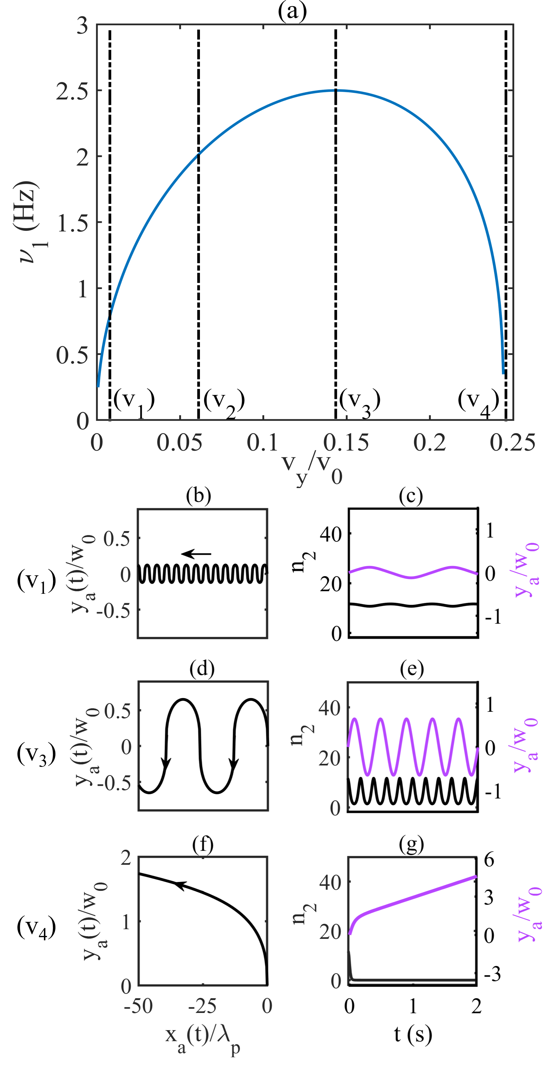
Next, we discuss how the snake state trajectories can be manipulated by controlling the initial speed $v_{y}$ of the atom, see Fig. 3. We plot the peak frequency $\nu_{1}$ of the Fourier transform of $y_{a}$ in Fig. 3(a) and observe two different regimes. Up to $v_{y}\approx 0.13v_{0}$, $\nu_{1}$ increases. In this regime, the oscillation amplitude along $y$-direction increases with increasing $v_{y}$ due to the increased initial speed and the amplitude of $n_{2}$ increases correspondingly as shown in Fig. 3(c, e). Such an increase of the oscillation amplitude implies that the particle sees higher average magnetic field which results in higher $\nu_{1}$ for higher initial $v_{y}$. The spatial period along the $x$-direction also increases leading to a faster transport of the atom, see Fig. 3(b,d).

For initial velocities higher than $0.13v_{0}$, $\nu_{1}$ decreases and amplitude of the snake state trajectories increases. At this point, the particle spans the region $|y|>w_{0}$ where the non-linear spatial structure of the magnetic field becomes important, see Fig. 1. The time evolution of $y_{a}$ also becomes complicated for a higher initial velocity and the corresponding Fourier transform shows weaker peaks at higher frequencies. For initial velocities beyond $v_{y}>0.24v_{0}$, the atom cannot be trapped along the $y$-direction by the synthetic magnetic field (see Fig. 3(f)) and the correspond photon number $n_{2}$ decays to zero as the particle leaves the cavity mode, see Fig. 3(g).

Figure 5: color online: For $g_{0}=2\pi\times 100$ MHz, we show the trajectories of the atom with and without feedback ($n_{1}=1000$ and $n_{2}=800$). The initial velocity $v_{x}=0$ and $v_{y}=0.06v_{0}$. The rest of the parameters are the same as considered in the preceding figures.

VI Cavity feedback induced breakdown of snake state trajectories

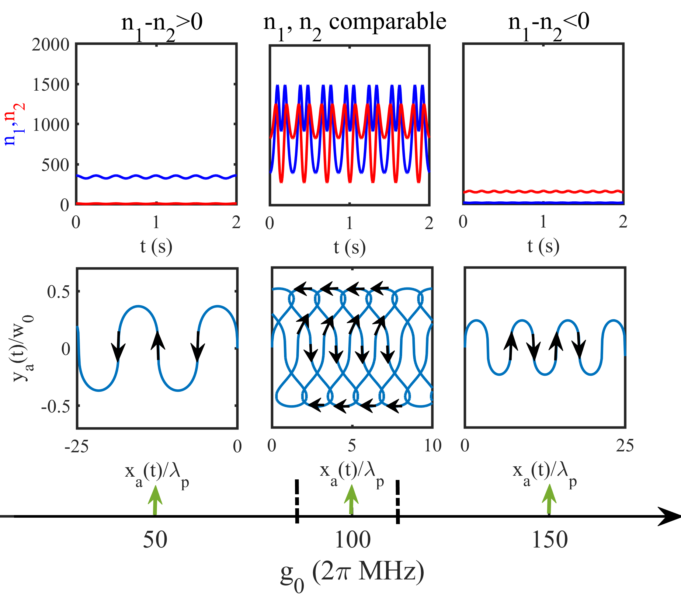
We now show how the number of photons in cavity mode 2 can be tuned by varying $g_{0}$ which allows us to control the direction of the snake states and even destroy them, see Fig. 4. Such a tuning of $n_{2}$ arises from $g_{0}^{2}$ dependence of $M_{0}$ and $P_{0}$ in Eq. (LABEL:alpha12). We observe three different regimes. For $g_{0}<<2\pi\times 100$ MHz, $n_{1}$ is greater than $n_{2}$ for all times and we observe left moving trajectories for $v_{y}>0$. This is the case discussed in previous sections. For $g_{0}>>2\pi\times 100$ MHz, $n_{2}$ is greater than $n_{1}$ at all times and hence we observe right moving snake state trajectories. In the critical regime with $g_{0}\approx 2\pi\times 100$ MHz, $n_{1}$ and $n_{2}$ are comparable and have complex time evolution. Thus, there is periodic reversal of the magnetic field direction (at a fixed $y$) which destroys the snake state trajectories. This is further illustrated in Fig. 5 where we compare the atomic trajectories with the cavity feedback to the case without feedback where the photon number is fixed to the time-averaged values of the feedback case. Similar, breakdown of snake state trajectories can be also achieved by pumping both the cavity modes such that $\eta_{1}\approx\eta_{2}$ leading to comparable photon number in the two cavity modes.

VII Conclusions and outlook

This work focuses on realizing atomic analogues of electronic snake-state trajectories in a ring-cavity system. We have shown that atom-cavity interaction gives rise to an effective spatially varying magnetic field that depends on the photon numbers in the two counter-propagating cavity modes. Atom in such a non-uniform magnetic field follows snake state trajectories and can be detected by monitoring the output cavity fields as they dynamically depend on the atom’s position. We can manipulate the different properties of snake states by changing the system parameters, such as the initial velocity of the atom, external pump strength, atom-cavity coupling strength, etc., to name a few. We can also tune the effect of cavity-backaction via atom-cavity coupling strength to change the topology of snake states and create even richer dynamics. As an extension of work, it will be interesting to study the effect of such synthetic magnetic field on an interacting Bose-Einstein condensate which has well-defined spatial phase and finite superfluid fraction. It will be also exciting to study how such synthetic magnetic field induced snake states compete with other well-known phenomena in high finesse ring cavities like superradiant Rayleigh scattering and collective recoil lasing [56].

VIII Acknowledgements

We thank Manuele Landini, Farokh Mivehvar, B. Prasanna Venkatesh, Mishkatul Bhattacharya and Puja Mondal, for a number of helpful discussions at various stages of this work. SG thanks the ETH group of T. Esslinger and P. Öhberg at Herriot-Watt University for helpful discussions during his visits there.This work is supported by a BRNS (DAE, Govt. of India) Grant No. 21/07/2015-BRNS/35041 (DAE SRC Outstanding Investigator scheme). PS was also supported by an UGC ( Govt. of India) fellowship at the initial stage of this work.

Appendix A Detailed derivation of the system Hamiltonian

The atomic and cavity part of the Hamiltonian are respectively given as -

$$\hat{H}_{A} = \frac{\vec{P}^{2}}{2m_{a}}\hat{\mathbb{I}}+\frac{\hbar\omega_{a}\hat{\sigma}_{z}}{2}$$ (8)

$$\hat{H}_{C} = \hbar\omega_{c}(\hat{a}_{1}^{\dagger}\hat{a}_{1}+\hat{a}_{2}^{\dagger}\hat{a}_{2})+\hbar\eta_{1}(\hat{a}_{1}e^{i\omega_{p}t}+\hat{a}_{1}^{{\dagger}}e^{-i\omega_{p}t})$$ (9)

$$+ \hbar\eta_{2}(\hat{a}_{2}e^{i\omega_{p}t}+\hat{a}_{2}^{{\dagger}}e^{-i\omega_{p}t})$$

Here $|g\rangle$ and $|e\rangle$ are respectively the ground and excited state of the two-level atom with energy $E_{g}$ and $E_{e}$, $\hat{\sigma}_{z}=|e\rangle\langle e|-|g\rangle\langle g|$ is the Pauli matrix, $E_{e}-E_{g}=\hbar\omega_{a}$, $\hat{\mathbb{I}}=|g\rangle\langle g|+|e\rangle\langle e|$ is the identity operator in the internal two-dimensional Hilbert space of the atom, $\vec{r}$ and $\vec{P}$ are the atomic centre-of-mass co-ordinate and momentum and $\omega_{p}$ is the pump frequency. The cavities are pumped on-axis with pump strengths $\eta_{1}$ and $\eta_{2}$. We also introduce $|\alpha_{1},\alpha_{2}\rangle$ to denote the coherent state for the photons of the two counter-propagating running wave modes as shown in Fig. 1 respectively labelled by the cavity field operators $\hat{a}_{1}$ and $\hat{a}_{2}$ with cavity resonance frequency, $\omega_{c}$. The single two-level excited atom scatters the photons into these two cavity modes.

The atom-cavity interaction is given as -

$$\hat{H}_{int.} = \hat{H}_{A-C}=-\vec{d}\cdot\vec{E}_{C}$$ (10)

where $\vec{d}=d(\hat{\sigma}^{+}+\hat{\sigma}^{-})$ is the dipole operator with $\hat{\sigma}^{+}=|e\rangle\langle g|$, and, $\hat{\sigma}^{-}=|g\rangle\langle e|$. $\hat{H}_{A-C}$ describes the interaction between the atom and the cavity fields (polarized along $y$ and $z$ directions) in one arm of the ring cavity, and its corresponding electric field is given by -

$$\vec{E}_{C}(\vec{r}) = \hat{e}_{y}\sqrt{\frac{\hbar\omega_{c}}{2\epsilon_{0}V}}e^{-y^{2}/w^{2}_{0}}\left(\hat{a}_{1}e^{ikx}+\hat{a}^{{\dagger}}_{1}e^{-ikx}\right)$$ (11)

$$+ \hat{e}_{z}\sqrt{\frac{\hbar\omega_{c}}{2\epsilon_{0}V}}e^{-y^{2}/w^{2}_{0}}\left(\hat{a}_{2}e^{-ikx}+\hat{a}^{{\dagger}}_{2}e^{ikx}\right)$$

Here $\epsilon_{0}$ is the vacuum permittivity, $V$ is the mode volume, $w_{0}$ is the beam waist, $k=\frac{2\pi}{\lambda_{p}}$, $\lambda_{p}$ is the pump wavelength and $\omega_{p}$ is the pump frequency. To get a clearer picture, we move to the interaction picture. The atomic field operators are given as $\hat{\sigma}^{\pm}(t)=\hat{\sigma}^{\pm}(0)e^{\pm i\omega_{a}t}$. The time evolution of the cavity field operators is found by solving the Heisenberg equation $i\hbar\frac{d\hat{a}_{1,2}}{dt}=[\hat{a}_{1,2},\hat{H}_{C}]=[\hat{a}_{1,2},\hbar\omega_{c}\hat{a}^{{\dagger}}_{1}\hat{a}_{1}+\hbar\omega_{c}\hat{a}^{{\dagger}}_{2}\hat{a}_{2}]$ and we obtain - $\hat{a}_{1,2}(t)=\hat{a}_{1,2}(0)e^{-i\omega_{c}t}$. Similarly, for $\hat{a}^{{\dagger}}_{1,2}$, we get - $\hat{a}_{1,2}^{{\dagger}}(t)=\hat{a}_{1,2}^{{\dagger}}(0)e^{i\omega_{c}t}$, where $\omega_{c}$ is the cavity resonance frequency. Using (11), the atom-cavity field interaction in the interaction picture is -

$$\hat{H}^{I}_{A-C} = -\vec{d}\cdot\vec{E}_{C}$$ (12)

$$= \hbar g_{1}(y)\Big{[}\hat{\sigma}^{+}(t)\hat{a}_{1}(t)e^{ikx}+\hat{\sigma}^{-}(t)\hat{a}_{1}(t)e^{ikx}$$

$$+ \hat{\sigma}^{+}(t)\hat{a}^{{\dagger}}_{1}(t)e^{-ikx}+\hat{\sigma}^{-}(t)\hat{a}_{1}^{{\dagger}}(t)e^{ikx}\Big{]}$$

$$+ \hbar g_{2}(y)\Big{[}\hat{\sigma}^{+}(t)\hat{a}_{2}(t)e^{-ikx}+\hat{\sigma}^{-}(t)\hat{a}_{2}(t)e^{-ikx}$$

$$+ \hat{\sigma}^{+}(t)\hat{a}^{{\dagger}}_{2}(t)e^{ikx}+\hat{\sigma}^{-}(t)\hat{a}^{{\dagger}}_{2}(t)e^{ikx}\Big{]}$$

If $\omega_{a}\sim\omega_{c}$, then the terms with $e^{\pm i(\omega_{a}-\omega_{c})t}$ will have small transition amplitudes that are proportional to $\frac{1}{(\omega_{a}+\omega_{c})^{2}}$. Therefore, the fast oscillating terms with frequency $\omega_{a}+\omega_{c}$ can be neglected as compared to the slow oscillating terms with frequency $\omega_{a}-\omega_{c}$. Transforming back to the Schrödinger picture we get [57, 58, 59] -

$$\boxed{\begin{aligned} \hat{H}_{A-C}&=&\hbar g_{1}(y)\left[\hat{\sigma}^{+}\hat{a}_{1}e^{ikx}+\hat{\sigma}^{-}\hat{a}_{1}^{{\dagger}}e^{-ikx}\right]\\ &+&\hbar g_{2}(y)\left[\hat{\sigma}^{+}\hat{a}_{2}e^{-ikx}+\hat{\sigma}^{-}\hat{a}^{{\dagger}}_{2}e^{ikx}\right]\end{aligned}}$$

The transformation to the rotating frame of the pump field is carried through the unitary operator,

$$\boxed{\hat{U}(t)=e^{-i\omega_{p}t(\frac{\hat{\sigma}_{z}}{2}+\hat{a}_{1}^{{\dagger}}\hat{a}_{1}+\hat{a}_{2}^{{\dagger}}\hat{a}_{2})}}$$

Since the observables and the states respectively transform as - $\hat{O}_{RF}=\hat{U}^{{\dagger}}\hat{O}\hat{U}$, and, $|\Psi_{RF}\rangle=\hat{U}^{{\dagger}}|\Psi\rangle$ in the rotating frame, the Schrödinger equation transforms as -

$$i\hbar\frac{\partial}{\partial t}|\Psi_{RF}\rangle =i\hbar\left[\frac{\partial}{\partial t}\left(\hat{U}^{{\dagger}}|\Psi\rangle\right)\right]=\hat{H}_{RF}|\Psi_{RF}\rangle$$

where

$$\hat{H}_{RF}=\frac{-\hbar\omega_{p}\hat{\sigma}_{z}}{2}-\hbar\omega_{p}\hat{a}^{{\dagger}}_{1}\hat{a}_{1}-\hbar\omega_{p}\hat{a}^{{\dagger}}_{2}\hat{a}_{2}+\hat{U}^{{\dagger}}\hat{H}_{SP}\hat{U}$$ (13)

is the single-particle Hamiltonian in the rotating frame of the pump field. To get $\hat{U}^{{\dagger}}\hat{H}_{SP}\hat{U}$, we use the Baker-Hausdorff formula which finally gives us

$$\hat{H}_{RF} = \frac{\hat{P}^{2}}{2m_{a}}\hat{\mathbb{I}}-\frac{\hbar\Delta_{a}\hat{\sigma}_{z}}{2}-\hbar\Delta_{c}\left(\hat{a}^{{\dagger}}_{1}\hat{a}_{1}+\hat{a}^{{\dagger}}_{2}\hat{a}_{2}\right)$$ (14)

$$+ \hbar\eta_{1}\left(\hat{a}^{{\dagger}}_{1}+\hat{a}_{1}\right)+\hbar\eta_{2}\left(\hat{a}^{{\dagger}}_{2}+\hat{a}_{2}\right)$$

$$+ \hbar g_{1}(y)\left[\hat{\sigma}^{+}\hat{a}_{1}e^{ikx}+\hat{\sigma}^{-}\hat{a}_{1}^{{\dagger}}e^{-ikx}\right]$$

$$+ \hbar g_{2}(y)\left[\hat{\sigma}^{+}\hat{a}_{2}e^{-ikx}+\hat{\sigma}^{-}\hat{a}^{{\dagger}}_{2}e^{ikx}\right]$$

where $\Delta_{a}=\omega_{p}-\omega_{a}$ is the atom-pump detuning and $\Delta_{c}=\omega_{p}-\omega_{c}$ is the cavity-pump detuning.

The resulting Hamiltonian in the rotating frame of the pump field is -

$$\hat{H}_{RF} = \hat{H}_{0}+\hat{H}_{I}$$ (15)

where

$$\hat{H}_{0} = \frac{\hat{P}^{2}}{2m_{a}}\hat{\mathbb{I}}$$

$$\hat{H}_{I} = -\frac{\hbar\Delta_{a}\hat{\sigma}_{z}}{2}-\hbar\Delta_{c}\left(\hat{a}^{{\dagger}}_{1}\hat{a}_{1}+\hat{a}^{{\dagger}}_{2}\hat{a}_{2}\right)$$

$$+ \hbar\eta_{1}\left(\hat{a}_{1}+\hat{a}^{{\dagger}}_{1}\right)+\hbar\eta_{2}\left(\hat{a}_{2}+\hat{a}^{{\dagger}}_{2}\right)$$

$$+ \hbar\left(g_{1}(y)\hat{\sigma}^{+}\hat{a}_{1}e^{ikx}+g_{2}(y)\hat{\sigma}^{+}\hat{a}_{2}e^{-ikx}\right.$$

$$+ \left.g_{1}(y)\hat{\sigma}^{-}\hat{a}^{{\dagger}}_{1}e^{-ikx}+g_{2}(y)\hat{\sigma}^{-}\hat{a}^{{\dagger}}_{2}e^{ikx}\right)$$

Here $g_{1}(y)=\frac{-\vec{d}\cdot\hat{e}_{y}}{\hbar}\sqrt{\frac{\hbar\omega_{c}}{2\epsilon_{0}V}}e^{-y^{2}/w^{2}_{0}}=g_{10}e^{-y^{2}/w^{2}_{0}}$, $g_{2}(y)=\frac{-\vec{d}\cdot\hat{e}_{z}}{\hbar}\sqrt{\frac{\hbar\omega_{c}}{2\epsilon_{0}V}}e^{-y^{2}/w^{2}_{0}}=g_{20}e^{-y^{2}/w^{2}_{0}}$, $\Delta_{a}=\omega_{p}-\omega_{a}$ is the atom-pump detuning, and, $\Delta_{c}=\omega_{p}-\omega_{c}$ is the cavity-pump detuning.

Appendix B Dressed states

The interaction Hamiltonian, $\hat{H}_{I}$ in the bare-state basis contains off-diagonal terms and can be written as -

$$\hat{H}_{I} = \begin{bmatrix}-\frac{\hbar}{2}\Delta_{a}+C_{t}&\hbar c_{1}\\ \hbar c^{*}_{1}&\frac{\hbar}{2}\Delta_{a}+C_{t}\\ \end{bmatrix}$$

where we have used
$C_{t}=-\hbar\Delta_{c}(|\alpha_{1}|^{2}+|\alpha_{2}|^{2})+2\hbar\eta_{1}|\alpha_{1}|\cos\theta_{1}+2\hbar\eta_{2}|\alpha_{2}|\cos\theta_{2}$, $c_{1}=g_{1}(y)\alpha_{1}e^{ikx}+g_{2}(y)\alpha_{2}e^{-ikx},$
$\hat{a}_{1,2}|\alpha_{1,2}\rangle=|\alpha_{1,2}|e^{i\theta_{1,2}}|\alpha_{1,2}\rangle$ and $\hat{a}^{{\dagger}}_{1,2}|\alpha_{1,2}\rangle=|\alpha_{1,2}|e^{-i\theta_{1,2}}|\alpha_{1,2}\rangle$

We diagonalise the Hamiltonian $\hat{H}_{I}$ in the space spanned by the atom-photon bare-states, namely $|e,\alpha_{1},\alpha_{2}\rangle,$ and $|g,\alpha_{1},\alpha_{2}\rangle$, and obtain the following eigenstates that are called dressed states $|D_{1}\rangle$ and $|D_{2}\rangle$, for the coupled atom-photon system, with $E_{1}$ and $E_{2}$ as their eigenvalues, respectively. They are

$$E_{1}=-\hbar\Delta_{c}(|\alpha_{1}|^{2}+|\alpha_{2}|^{2})+2\hbar\eta_{1}|\alpha_{1}|\cos\theta_{1}+2\hbar\eta_{2}|\alpha_{2}|\cos\theta_{2}-\frac{\hbar G}{2};$$ (17a)

$$|D_{1}\rangle = \frac{1}{\sqrt{2G(G+\Delta_{a})}}\begin{bmatrix}G+\Delta_{a}\\ -2c^{*}_{1}\end{bmatrix}$$ (17b)

$$E_{2}=-\hbar\Delta_{c}(|\alpha_{1}|^{2}+|\alpha_{2}|^{2})+2\hbar\eta_{1}|\alpha_{1}|\cos\theta_{1}+2\hbar\eta_{2}|\alpha_{2}|\cos\theta_{2}+\frac{\hbar G}{2};$$ (17c)

$$|D_{2}\rangle = \frac{1}{\sqrt{2G(G+\Delta_{a})}}\begin{bmatrix}2c_{1}\\ G+\Delta_{a}\end{bmatrix}$$ (17d)

where

$$|c_{1}|^{2} = \left(g_{1}^{2}(y)|\alpha_{1}|^{2}+g_{2}^{2}(y)|\alpha_{2}|^{2}\right)$$

$$G = \sqrt{\Delta_{a}^{2}+4|c_{1}|^{2}}$$

Appendix C Equation of Motion and action of momentum operator on the atomic wave-function

In the dressed state basis ($\ket{D_{i}}$ basis) for the internal Hilbert space of the atom at any point $\vec{r}$, the full state vector of the atom and the corresponding equation of motion is -

$$|\Psi(\vec{r},t)\rangle=\sum_{j=1,2}\psi_{j}(\vec{r},t)|D_{j}\rangle$$ (18)

$$i\hbar\frac{\partial}{\partial t}|\Psi(\vec{r},t)\rangle=\hat{H}_{RF}|\Psi(\vec{r},t)\rangle$$ (19)

We provide the detailed derivation to find out the action of the momentum operator, $\hat{P}$, on the atomic wavefunction, $|\Psi(\vec{r},t)\rangle$.

$$\hat{P}|\Psi(\vec{r},t)\rangle = -i\hbar\vec{\nabla}\left[\sum_{j=1,2}\psi_{j}(\vec{r},t)|D_{j}\rangle\right]$$ (20)

$$= -i\hbar\sum_{j}\left[(\vec{\nabla}\psi_{j}(\vec{r},t))|D_{j}\rangle+\psi_{j}(\vec{r},t)(\vec{\nabla}|D_{j}\rangle)\right]$$

$$= \sum_{j,l=1,2}\left[\vec{p}\delta_{l,j}-\vec{\textbf{A}}_{l,j}\right]\psi_{j}|D_{l}\rangle$$

where $\vec{\textbf{A}}_{l,j}=i\hbar\langle D_{l}|\vec{\nabla}|D_{j}\rangle$ is the vector potential and $\vec{p}=-i\hbar\vec{\nabla}=$ does not act on the spinorial part. From this, we can straightforwardly write the kinetic energy term as

$$\frac{\vec{P}^{2}}{2m_{a}}|\Psi(\vec{r},t)\rangle=\frac{1}{2m_{a}}\sum_{j,l,m=1,2}\Big{\{}\left(\vec{p}\delta_{l,j}-\vec{\textbf{A}}_{l,j}\right)\left[\left(\vec{p}\delta_{m,l}-\vec{\textbf{A}}_{m,l}\right)\psi_{j}\right]\Big{\}}|D_{m}\rangle$$ (21)

We can write down a matrix $\vec{\textbf{A}}$ whose components are given as - $\vec{\textbf{A}}_{l,j}=i\hbar\langle D_{l}|\vec{\nabla}|D_{j}\rangle$

$$\vec{\textbf{A}} = i\hbar\begin{bmatrix}\langle D_{1}|\vec{\nabla}|D_{1}\rangle&\langle D_{1}|\vec{\nabla}|D_{2}\rangle\\ \langle D_{2}|\vec{\nabla}|D_{1}\rangle&\langle D_{2}|\vec{\nabla}|D_{2}\rangle\end{bmatrix}$$

We project the Schrödinger equation to the lowest energy dressed state -

$$\langle D_{1}|i\hbar\frac{\partial}{\partial t}|\Psi(\vec{r},t)\rangle = \langle D_{1}|\hat{H}_{RF}|\Psi(\vec{r},t)\rangle$$ (22)

LHS of Eq.(22) gives -

$$\langle D_{1}|i\hbar\frac{\partial}{\partial t}|\Psi(\vec{r},t)\rangle = \langle D_{1}|i\hbar\frac{\partial}{\partial t}\sum_{j=1}\psi_{j}(\vec{r},t)|D_{j}\rangle$$ (23)

$$= i\hbar\sum_{j=1}\langle D_{1}|\frac{\partial}{\partial t}\psi_{j}(\vec{r},t)|D_{j}\rangle$$

$$= i\hbar\frac{\partial}{\partial t}\psi_{1}(\vec{r},t)$$

RHS of Schrödinger Eq.(22) is -

$$\langle D_{1}|\hat{H}_{RF}|\Psi(\vec{r},t)\rangle = \langle D_{1}|\left[\left(\frac{\hat{P}^{2}}{2m_{a}}\right)\hat{\mathbb{I}}+\hat{H}_{I}\right]|\Psi(\vec{r},t)\rangle$$

The first term of Eq.(LABEL:appenRHS) gives -

$$\langle D_{1}|\frac{\vec{P}^{2}}{2m_{a}}|\Psi(\vec{r},t)\rangle = \frac{1}{2m_{a}}\sum_{j=1;l,m=1,2}\left(\{\left(\vec{p}\delta_{l,j}-\vec{\textbf{A}}_{l,j}\right)\left[\left(\vec{p}\delta_{m,l}-\vec{\textbf{A}}_{m,l}\right)\psi_{j}\right]\}\langle D_{1}|D_{m}\rangle\right)$$

$$= \frac{1}{2m_{a}}\Big{\{}\left(\vec{p}-\vec{\textbf{A}}_{1,1}\right)^{2}+|\vec{\textbf{A}}_{2,1}|^{2}\Big{\}}\psi_{1}(\vec{r},t)$$

The second term of Eq.(LABEL:appenRHS), gives -

$$\langle D_{1}|\hat{H}_{I}|\Psi(\vec{r},t)\rangle = E_{1}\psi_{1}(\vec{r},t)$$

From Eq.(23) and Eq.(LABEL:appenRHS), we obtain the equation for the probability amplitude, $\psi_{1}$, to find the atom in the lowest energy dressed state, $|D_{1}\rangle$ -

$$i\hbar\frac{\partial}{\partial t}\psi_{1}(\vec{r},t)=H_{S}\psi_{1}(\vec{r},t)=\Big{[}\frac{1}{2m_{a}}\Big{\{}\left(\vec{p}-\vec{\textbf{A}}_{1,1}\right)^{2}+|\vec{\textbf{A}}_{2,1}|^{2}\Big{\}}+E_{1}\Big{]}\psi_{1}(\vec{r},t)$$ (25)

Appendix D Semi-classical equation of motion

The Hamiltonian for the system can be written as -

$$\hat{H}=\frac{\hat{P}^{2}}{2m_{a}}+\hat{V}(\vec{r})$$ (26)

where the effective potential $\hat{V}(\vec{r})$ is given as

$$\hat{V}(\vec{r})=\sum_{j=1,2,3}E_{j}(\vec{r})\hat{Q}_{j}(\vec{r})$$ (27)

with $\hat{Q}_{j}(\vec{r})=|D_{j}(\vec{r})\rangle\langle D_{j}(\vec{r})|$ is the projector onto the $j^{th}$-eigenstate of the atom-field coupling. The force operator in this Hilbert space is

$$\hat{F}(\vec{r}) = -\vec{\nabla}\hat{V}(\vec{r})$$

$$= -\sum_{j}\left[\left(\vec{\nabla}E_{j}(\vec{r})\right)\hat{Q}_{j}(\vec{r})+E_{j}(\vec{r})\left(\vec{\nabla}\hat{Q}_{j}(\vec{r})\right)\right]$$

with the expectation value $\langle\hat{F}\rangle$ is then given by $\langle\hat{F}\rangle=\langle\Psi|\hat{F}(\vec{r})|\Psi\rangle$ where $|\Psi(\vec{r},t)\rangle=\sum_{j=1,2}\psi_{j}(t)|D_{j}(\vec{r}(t))\rangle$ comes out to be [53] -

$$\langle\hat{F}(\vec{r},t)\rangle=-\sum_{j}|\psi_{j}|^{2}\vec{\nabla}E_{j}+\sum_{j,k}\psi^{*}_{j}\psi_{k}(E_{k}-E_{j})\langle D_{k}|\vec{\nabla}D_{j}\rangle$$ (29)

To obtain the force at first order in $\vec{v}$, we have to find out all the coefficients, $\psi_{j}$ at first order. The Schrödinger equation for $|\Psi(\vec{r},t)\rangle$ is [53]-

$$i\hbar|\dot{\Psi}(\vec{r},t)\rangle=\hat{V}(\vec{r},t)|\Psi(\vec{r},t)\rangle$$ (30)

and

$$|\dot{\Psi}(\vec{r},t)\rangle = \frac{d}{dt}\left(\sum_{j}\psi_{j}(t)|D_{j}(\vec{r}(t))\rangle\right)$$ (31)

$$= \sum_{j}\dot{\psi}_{j}|D_{j}\rangle+\sum_{j}\psi_{j}\vec{v}\cdot|\vec{\nabla}D_{j}\rangle$$

We get the corresponding equation of motion for $\psi_{j}$ as -

$$\dot{\psi}_{j}=-iE_{j}\frac{\psi_{j}}{\hbar}+\sum_{k}\psi_{j}\vec{v}\cdot\langle D_{j}|\vec{\nabla}D_{k}\rangle$$ (32)

At order zero, we get $\psi_{1}=e^{-iE_{1}t/\hbar}$ and $\psi_{2},\psi_{3}=0$.
At first order in $\vec{v}$, the equation of motion for $\psi_{1}$ is -

$$\dot{\psi}_{1}=-i\left(E_{1}-\vec{v}\cdot\vec{A}\right)\psi_{1}/\hbar$$ (33)

whose solution is a number of modulus 1. For $j\neq 1$ (assuming adiabatic motion of the atom, i.e., $T\left(E_{j}-E_{1}\right)/\hbar>>1$), we get -

$$\psi_{j}(T)\simeq i\hbar\frac{\vec{v}\cdot\langle D_{j}|\vec{\nabla}D_{1}\rangle}{E_{j}-E_{1}}e^{-iE_{1}T/\hbar}$$ (34)

We see that first term of $\langle\hat{F}\rangle$ in Eq.(29), has no first-order component in $\vec{v}$, since the contributions of $\psi_{j}^{\prime}s$ for $j\neq 1$ are at least of order 2 and the contribution of $\psi_{1}$ is independent of $\vec{v}$. In the second term of Eq.(29), the relevant terms are the ones where one of two indices $j$ or $k$ is 1. Applying the closure property, and keeping terms up to first order in $\vec{v}$, we get $\langle\hat{F}\rangle=i\hbar\langle\vec{\nabla}D_{1}|\left(\vec{v}\cdot|\vec{\nabla}D_{1}\rangle\right)+c.c.$. This expression gives the Lorentz force $\vec{v}\times\vec{B}$ in the equation of motion. The semi-classical equation of motion for the atom in the lowest energy dressed state can now be given as -

$$m_{a}\frac{d\vec{v}}{dt}=-\vec{\nabla}E_{1}-\vec{\nabla}W(\vec{r})+\vec{v}\times\vec{B}(\vec{r})$$ (35)

Figure A.1: color online: (a) Photon numbers in cavity mode 1, $n_{1}$ $(blue$ curve) as a function of $t$. (b) Fourier transform of $n_{1}$ shows peaks at $2\nu_{0}$, $4\nu_{0}$, $6\nu_{0}$ and so on.

Appendix E Photon numbers in mode 1 and their phase $\phi_{1}$

We provide the plots for the photon numbers in mode 1 and its Fourier transform which shows a peak at $2\nu_{0}$ in Fig.A.1. The peaks at $4\nu_{0}$ and $6\nu_{0}$ are not visible.

References

- [1] Many-body physics with ultracold gases, I. Bloch, J. Dalibard, and W. Zwerger, Rev. Mod. Phys. 80, 885 (2008).
- [2] Quantum Simulators, I. Buluta and F. Nori, Science 326, 108 (2009).
- [3] Ultra cold quantum gases in optical lattices, I. Bloch, Nature Phys. 1, 23 (2005).
- [4] Quantum wires and quantum dots for neutral atoms J. Schmeidmayer, Eur. Phys. J. D 4, 57(1998).
- [5] Quantum gas microscopy for single atom and spin detection, C. Gross and W. S. Bakr, Nat. Phys. 17, 1316(2021).
- [6] Quantum science with optical tweezer arrays of ultracold atoms and molecules, A. M. Kaufman and K.-K. Ni, Nat. Phys. 17, 1324(2021).
- [7] Colloquium: Artificial gauge potentials for neutral atoms, J. Dalibard, F. Gerbier, G. Juzeliũnas and P. Öhberg, Rev. Mod. Phys., 83, 1523 (2011).
- [8] Light-induced gauge fields for ultracold atoms, N. Goldman, G. Juzeliũnas, P. Öhberg, and I. B. Spielman, Rep. Prog. Phys. 77, 126401 (2014).
- [9] Raman processes and effective gauge potentials, I. B. Spielman, Phys. Rev. A 79,063613 (2009).
- [10] Gauge fields for ultracold atoms in optical superlattices, F. Gerbier and J. Dalibard, New Journal of Physics, 12(3), 033007(2010).
- [11] Creation of effective magnetic fields in optical lattices: the Hofstadter butterfly for cold neutral atoms, D. Jaksch and P. Zoller, New J. Phys. 5, 56 (2003); Fractional Quantum Hall States of Atoms in Optical Lattices, A. S. Sorensen, E. Demler, and M. D. Lukin, Phys. Rev. Lett. 94, 086803 (2005).
- [12] Creating artificial magnetic fields for cold atoms by photon-assisted tunneling, A. R. Kolovsky, Europhys. Lett. 93, 20003 (2011); Optical Flux Lattices for Ultracold Atomic Gases, N. R. Cooper, Phys. Rev. Lett. 106, 175301 (2011); Quantum Simulation of Frustrated Classical Magnetism in Triangular Optical Lattices, J. Struck, C. Ölschläger, R. Le Targat, P. Soltan-Panahi, A. Eckardt, M. Lewenstein, P. Windpassinger, and K. Sengstock, Science 333, 996 (2011); Experimental Realization of Strong Effective Magnetic Fields in an Optical LatticeM. Aidelsburger, M. Atala, S. Nascimbène, S. Trotzky, Y.-A. Chen, and I. Bloch, Phys. Rev. Lett. 107, 255301 (2011).
- [13] Non-Abelian Gauge Fields and Topological Insulators in Shaken Optical Lattices, P. Hauke, O. Tieleman, A. Celi, C. Ölschlöger, J. Simonet, J. Struck, M. Weinberg, P. Windpassinger, K. Sengstock, M. Lewenstein, and A. Eckardt, Phys. Rev. Lett. 109, 145301 (2012); Tunable Gauge Potential for Neutral and Spinless Particles in Driven Optical Lattices, J. Struck, C. ÖlschlÄger, M. Weinberg, P. Hauke, J. Simonet, A. Eckardt, M. Lewenstein, K. Sengstock, and P. Windpassinger, Phys. Rev. Lett. 108, 225304 (2012).
- [14] Realizing the Harper Hamiltonian with Laser-Assisted Tunneling in Optical Lattices, H. Miyake, G. A. Siviloglou, C. J. Kennedy, W. C. Burton, and W. Ketterle, Phys. Rev. Lett. 111, 185302 (2013); Realization of the Hofstadter Hamiltonian with Ultracold Atoms in Optical Lattices, M. Aidelsburger, M. Atala, M. Lohse, J. T. Barreiro, B. Paredes, and I. Bloch, Phys. Rev. Lett. 111, 185301 (2013).
- [15] Bose-Einstein Condensate in a Uniform Light-Induced Vector Potential, Y.-J. Lin, R. L. Compton, A. R. Perry, W. D. Phillips, J. V. Porto, and I. B. Spielman, Phys. Rev. Lett. 102, 130401 (2009); Spin–orbit-coupled Bose–Einstein condensates, Y.-J. Lin, R. L. Compton, K. Jimenez-Garcia, J. V. Porto, and I. B. Spielman, Nature (London) 462, 628 (2009).
- [16] Synthetic spin-orbit interactions and magnetic fields in ring-cavity QED, F. Mivehvar and D. L. Feder, Phys. Rev. A 89, 013803 (2014).
- [17] Effect of a Nonuniform Magnetic Field on a Two-Dimensional Electron Gas in the Ballistic Regime, J. E. Müller, Phys. Rev. Lett. 68, 385 (1992).
- [18] Electrons in a Periodic Magnetic Field Induced by a Regular Array of Micromagnets, P. D. Ye, D. Weiss, R. R. Gerhardts, M. Seeger, K. von Klitzing, K. Eberl and H. Nickel, Phys. Rev. Lett. 74, 3013 (1995).
- [19] Snake States along Graphene p-n Junctions, J. R. Williams and C. M. Marcus, Phys. Rev. Lett. 107, 046602 (2011).
- [20] Snake trajectories in ultraclean graphene p-n junctions, P. Rickhaus, P. Makk, M.-H. Liu, E. Tovari, M. Weiss, R. Maurand, K. Richter and C. Schönenberger, Nat. Comm. 6, Article number: 6470 (2015).
- [21] Snake orbits and related magnetic edge states, J. Reijneirs and F. M. Peeters J. Phys.:Condens. Matter 12, 9771 (2000).
- [22] Confined magnetic guiding orbit states, J. Reijniers, A. Matulis, K. Chang, F. M. Peeters and P. Vasilopoulos, Europhys. Lett., 59(5), 749(2002).
- [23] Electron dynamics in inhomogeneous magnetic fields, A. Nogaret, J. Phys.: Cond. Matter, 22, 253201 (2010).
- [24] Theory of snake states in graphene, L. Oroszlány, P. Rakyta, A. Kormányos, C. J. Lambert, and J. Cserti, Phys. Rev. B, 77, 081403(R)(2008).
- [25] Conductance quantization and snake states in graphene magnetic waveguides, T. K. Ghosh, A. De Martino, W. Häusler, L. Dell’Anna, and R. Egger, Phys. Rev. B, 77, 081404(R) (2008).
- [26] Magnetic edge states in graphene in nonuniform magnetic fields, S. Park and H.-S. Sim, Phys. Rev. B, 77, 075433 (2008).
- [27] Crossover between magnetic and electric edges in quantum Hall systems, A. Nogaret, P. Mondal, A. Kumar, S. Ghosh, H Beere and D. Ritchie, Phys. Rev. B 96, 081302(R) (2017).
- [28] Quantum transport through pairs of edge states of opposite chirality at electric and magnetic boundaries, P. Mondal, A. Nogaret and S. Ghosh, Phys. Rev. B 98, 125303 (2018).
- [29] Microscopic atom optics: from wires to an atom chip, R. Folman, P. Kruger, J. Schmiedmayer, J. Denschlag, and C. Henkel, Adv. At. Mol., Opt. Phys. 48, 263 (2002).
- [30] Atomtronics: Ultracold-atom analogues of electronic devices, B. T. Seaman, M. Krämer, D. Z. Anderson, and M. J. Holland , Phys. Rev. A 75, 023615 (2007).
- [31] Focus on atomtronics-enabled quantum technologies , L. Amico, G. Birkl, M. Boshier, and L.-C. Kwek, New J. Phys. 19, 020201 (2017).
- [32] Optical lattices, ultracold atoms and quantum information processing, D. Jaksch, Contemporary Physics, 45(5), 367(2004)
- [33] Observation of quantum-measurement backaction with an ultracold atomic gas, K. W. Murch, K. L. Moore, S. Gupta and D. M. Stamper-Kurn , Nature Physics 4, 561-564 (2008).
- [34] Dicke quantum phase transition with a superfluid gas in an optical cavity, K. Baumann, C. Gulerin, F. Brennecke and T. Esslinger, Nature 464, 1301 (2010).
- [35] Supersolid formation in a quantum gas breaking a continuous translational symmetry, J. Léonard, A. Morales, P. Zupancic, T. Esslinger, and T. Donner, Nature (London) 543, 87 (2017).
- [36] An optical lattice with sound, Y. Guo, et al., Nature, 599, 211 (2022).
- [37] Meissner-like Effect for a Synthetic Gauge Field in Multimode Cavity QED, K. E. Ballantine, B. Lev and J. Keeling, Phys. Rev. Lett. 118, 045302 (2017).
- [38] H. Ritsch, P. Domokos, F. Brennecke and T. Esslinger, Rev. of Mod. Phys., 85, 553 (2013).
- [39] F. Mivehvar, F. Piazza, T. Donner and H. Ritsch, Adv. in Phys. 70, 1 (2021).
- [40] Comparison of Quantum and Semiclassical Radiation Theories with Application to the Beam Maser , E. T. Jaynes and F. W. Cummings, Proc. IEEE 51, 89-109(1963).
- [41] M. Born, R. Oppenheimer, Ann. Physik 84, 457(1930).
- [42] On the determination of Born-Oppenheimer nuclear motion wave functions including complications due to conical intersections and identical nuclei, C.A. Mead, D.G. Truhlar, J. Chem. Phys. 70, 2284 (1979).
- [43] Quantal phase factors accompanying adiabatic changes, M.V. Berry, Proc. R. Soc. Lond. A 392, 45 (1984).
- [44] Appearance of Gauge Structure in Simple Dynamical Systems, F. Wilczek and A. Zee, Phys. Rev. Lett. 25, 2111 (1984).
- [45] Realizations of Magnetic-Monopole Gauge Fields: Diatoms and Spin Precession, J. Moody, A. Shapere, and F. Wilczek, Phys. Rev. Lett. 56, 893 (1986).
- [46] Molecular Kramers Degeneracy and Non-Abelian Adiabatic Phase Factors, C.A. Mead, Phys. Rev. Lett. 59, 161 (1987).
- [47] Geometric Phases in Physics, edited by A. Shapere, F. Wilczek (World Scientific, Singapore, 1989.)
- [48] High-order quantum adiabatic approximation and Berry’s phase factor, C.P. Sun, J. Phys. A: Math. Gen. 21, 1595 (1988).
- [49] Generalizing Born-Oppenheimer approximations and observable effects of an induced gauge field, C.P. Sun and M.L. Ge, Phys. Rev. D 41, 1349 (1990).
- [50] Trapping Atoms by the Vacuum Field in a Cavity, S. Haroche, M. Brune and J. M. Raimond, Europhys. Lett., 14(l), 19 (1991).
- [51] Artificial gauge potentials for neutral atoms: an application in evanescent light fields, V. E. Lembessis, J. Opt. Soc. Am. B 31, 1322 (2014).
- [52] Artificial magnetic field induced by an evanescent wave, M. Mochol and K. Sacha, Sci. Rep. 5, Article number: 7672 (2015).
- [53] Geometric potentials in quantum optics: A semiclassical interpretation, M. Cheneau, S. P. Rath, T. Yefsah, K. J. Günter, G. Juzeliunas and J. Dalibard, Eur. Phys. Lett. 83, 60001(2008).
- [54] L. D. Landau and E. M. Lifshitz, The classical theory of fields, Chapter 3, Pergamon Press (1998).
- [55] J. D. Jackson, Classical Electrodynamics, Wiley, New York (1962).
- [56] Superradiant Rayleigh Scattering and Collective Atomic Recoil Lasing in a Ring Cavity, S. Slama, S. Bux, G. Krenz, C. Zimmermann, and Ph.W. Courteille. Phys. Rev. Lett., 98, 053603 (2007).
- [57] Is a quantum standing wave composed of two travelling waves, B. W. Shore, P. Meystre and S. Stenholm, J. Opt. Soc. Am. B, 8(4), 903(1991).
- [58] J. J. Sakurai, Modern Quantum Mechanics, Revised Edition, ed. S. F. Tuan, (Addison-Wesley Publishing Company, 1994).
- [59] Coupled harmonic systems as quantum buses in thermal environments, F. Nicacio and F. L. Semiao, J. Phys. A: Math. Theor. 49, 375303(2016). (See Appendix A)