Towards a complete description of spectra and polarization of black hole accretion disks: albedo profiles and returning radiation

Abstract

Accretion disks around stellar-mass black holes (BHs) emit radiation peaking in the soft X-rays when the source is in the thermal state. The emerging photons are polarized and, for symmetry reasons, the polarization integrated over the source is expected to be either parallel or perpendicular to the (projected) disk symmetry axis, because of electron scattering in the disk. However, due to General Relativity effects photon polarization vectors will rotate with respect to their original orientation, by an amount depending on both the BH spin and the observer’s inclination. Hence, X-ray polarization measurements may provide important information about strong gravity effects around these sources. Along with the spectral and polarization properties of radiation which reaches directly the observer once emitted from the disk, in this paper we also include the contribution of returning radiation, i.e. photons that are bent by the strong BH gravity to return again on the disk, where they scatter until eventually escaping to infinity. A comparison between our results and those obtained in previous works by different authors show an overall good agreement, despite the use of different code architectures. We finally consider the effects of absorption in the disk material by including more realistic albedo profiles for the disk surface. Our findings in this respect show that considering also the ionization state of the disk may deeply modify the behavior of polarization observables.

1 Introduction

Black holes (BHs) are the most compact astrophysical objects, which can be used as ideal laboratories to test physics in the presence of ultra-strong graviational fields. Different kinds of BHs have been identified so far and classified according to their mass. Stellar-mass BHs ($M\approx 10\,M_{\odot}$) are believed to be born mainly in the gravitational core-collapse of stars with a initial mass $\ga 25$–$30\,M_{\odot}$ (see Woosley, Heger & Weaver, 2002, for a review). On the other hand, the different observational manifestations of active galactic nuclei (AGN) have been explained with the presence of supermassive BHs ($M\approx$ $10^{6}$–$10^{9}\,M_{\odot}$, see e.g. Salpeter, 1964; Zel’dovich & Novikov, 1964; Lynden-Bell, 1969), which have been observed to be hosted in centers of most galaxies, including our own Milky Way (see Kormendy & Ho, 2013; Graham, 2016). Finally, intermediate-mass BHs ($M\approx 10^{2}$–$10^{5}\,M_{\odot}$) have been also reported in some dim AGN or associated to ultra-luminous X-ray sources (see Mezcua, 2017, for a recent review).

Despite the fact that even light cannot escape from their event horizon, BHs have been observed so far as X-ray sources, through the electromagnetic radiation emitted from accretion disks in binary systems, as well as, in the case of intermediate and supermassive BHs, by studying the orbits of nearby objects (stars) influenced by the presence of their gravitational field (as in the case of the supermassive BH at the Galactic center, see Schödel et al., 2002). Very recently, BHs have been in the spotlight thanks to the results achieved by the LIGO/VIRGO collaboration, which detected for the first time the gravitational waves emitted in BH-BH merging events Abbott et al. (2016). Nevertheless, electromagnetic observations still play a key role in understanding the physics of BHs.

General relativity plays a fundamental role in the physical processes that occur in the BH environment. The trajectories of photons which propagate close to a BH, for example, deviate from straight lines, following null geodesics that can be described in the proper space-time metric Bardeen (1970). Moreover, photon frequencies turn out to be gravitationally red-shifted as a result of the BH potential well, whereas the Doppler effect changes the photon frequency either way depending on the state of motion of the source with respect to the observer (Bardeen, Press & Teukolsky 1972). However, strong gravity also influences the polarization states of photons. In fact, the polarization vectors are generally rotated, with respect to their original orientation, because of the parallel transport along null geodesics. The recent developments in X-ray polarimetry techniques Costa et al. (2001); Bellazzini et al. (2010) gave indeed new impetus to this field of research.

Theoretical models to investigate spectra and polarization from these sources have been developed by many authors in the past (see e.g. Laor et al., 1990; Matt et al., 1993; Rauch & Blandford, 1994; Bao et al., 1997; Agol & Krolik, 2000; Li et al., 2005, 2009; Karas, 2006, and Schnittman & Krolik 2013 for a comprehensive list of further references). Furthermore, spectral and polarimetric studies on radiation coming from accretion disks and atmospheres in the case of AGN (either magnetized or not) have been carried out by Silant’ev et al. (2009, see also ). In the present paper we revisit in particular the work by Dovčiak et al. (2008), first incorporating in their original treatment the contribution of “returning radiation”, i.e. photons which are forced by the strong BH gravity to return to the disk before reaching the observer at infinity. This issue has been already addressed by Schnittman & Krolik (2009, see also ), who exploited a Monte Carlo code (exhaustively described in Schnittman & Krolik, 2013, see also Schnittman et al. 2013) to properly take into account both vacuum transport and radiative processes that influence photon propagation around stellar-mass BHs. While we adopt Kerr metric in the present paper, we will also refer to the study carried out by Krawczynski (2012), who instead developed a ray-tracing code capable to give predictions for different kinds of space-time metrics.

Although a complete, self-consistent treatment of ionization is still deferred to a future work, we move a step towards the inclusion in the model of a realistic ioniziation profile of the disk material. To this aim we convolve the output of our code with a non-trivial prescription for the disk albedo, obtained using the external code cloudy Ferland et al. (2017). The results show that both spectral and polarization properties of BH accretion disk emission are considerably modified by considering absorption in the disk with respect to the simple case of $100\%$ albedo. For this reason, in order to correctly interpret the physical and geometrical information that can be extracted from these sources using X-ray polarimetry, a proper study of the optical properties of the disk is required. This acquires even more significance in the light of the launch of the NASA-SMEX mission IXPE Weisskopf et al. (2013), scheduled for 2021, which will be capable of probing X-ray polarimetric properties of bright accreting black hole binaries.

The plan of the paper is as follows. In section 2 we briefly set up the theoretical model and present our main assumptions, while an overview of the numerical implementation is described in section 3. Results are then illustrated in section 4: in particular, the outputs of our codes are compared with the results previously obtained by Schnittman & Krolik (2009) and Krawczynski (2012) in §4.1; the effect of changing the optical depth of the electron-dominated atmosphere assumed to cover the disk surface are discussed in §4.2; and the results obtained considering a different albedo prescription for the disk are presented in §4.3. Finally, we summarize our findings and present our conclusions in section 5.

2 The model

We consider in this work only accretion disks around stellar-mass BHs in their thermal state, which are observed to emit radiation peaking in the soft X-rays (at about $1$ keV, see e.g. Schnittman & Krolik, 2009). The space-time around the central BH is described by the Kerr metric, for different values of its dimensionless angular momentum per unit mass $a$.

We treat the accretion disk as a geometrically-thin standard disk Shakura & Sunayev (1973). In particular, in order to dissipate their angular momentum, particles on the disk are assumed to rotate around the central BH with a Keplerian velocity. Photons are assumed to be emitted from the disk according to an isotropic blackbody (BB) distribution at different temperatures, following a Novikov-Thorne radial profile (a multicolor disk, see Novikov & Thorne, 1973; Wang, 2000, see also Cunningham 1975 for a more complete relativistic treatment),

$$T(M,r,a) =741f_{\rm col}\left(\frac{M}{M_{\odot}}\right)^{-1/2}\left(\frac{\dot{M}}{M_{\odot}/{\rm yr}}\right)^{1/4}$$

$$\ \ \ \ \times\big{[}f(\xi,a)\big{]}^{1/4}\,{\rm keV}\,,$$ (1)

where $M$ is the BH mass, $\dot{M}$ is the mass accretion rate, $\xi=(r/r_{\rm g})^{1/2}$, with $r$ the radial coordinate and $r_{\rm g}=GM/c^{2}$ the gravitational radius, and (see Page & Thorne, 1974)

$$f(\xi,a) =\frac{1}{\xi^{4}(\xi^{3}-3\xi+2a)}\left[\xi-\xi_{\rm ms}-\frac{3}{2}a\ln\left(\frac{\xi}{\xi_{\rm ms}}\right)\right.$$

$$\ \ -\frac{3(\xi_{1}-a)^{2}}{\xi_{1}(\xi_{1}-\xi_{2})(\xi_{1}-\xi_{3})}\ln\left(\frac{\xi-\xi_{1}}{\xi_{\rm ms}-\xi_{1}}\right)$$

$$\ \ -\frac{3(\xi_{2}-a)^{2}}{\xi_{2}(\xi_{2}-\xi_{1})(\xi_{2}-\xi_{3})}\ln\left(\frac{\xi-\xi_{2}}{\xi_{\rm ms}-\xi_{2}}\right)$$

$$\ \ \left.-\frac{3(\xi_{3}-a)^{2}}{\xi_{3}(\xi_{3}-\xi_{1})(\xi_{3}-\xi_{2})}\ln\left(\frac{\xi-\xi_{3}}{\xi_{\rm ms}-\xi_{3}}\right)\right]\,,$$ (2)

with $\xi_{1,2}=2\cos[(\arccos{a}\mp\pi)/3]$, $\xi_{3}=-2\cos[(\arccos{a})/3]$ and $\xi_{\rm ms}=(r_{\rm ms}/r_{\rm g})^{1/2}$, where $r_{\rm ms}$ is the radius of the innermost stable circular orbit (ISCO, see Bardeen et al., 1972). The hardening factor $f_{\rm col}$ is adopted to shift the energy of the thermal photons emerging from the disk in order to account (in a simplified way) for the effects of scatterings they undergo with disk particles (see Dovčiak et al., 2008; Davis & El-Abd, 2019). We also assumed no-torque at the inner edge of the disk, which is taken as coincident with the ISCO.

Photons emitted from the disk are expected to be linearly polarized essentially due to scatterings that occur onto the particles which compose the disk. In this respect, we assume that the photon polarization states follow the Chandrasekhar profile (see e.g. Chandrasekhar, 1960); this amounts to consider a pure-electron, scattering dominated atmospheric layer that covers the disk surface. Symmetry considerations lead to two possible polarization states, with the polarization vector either parallel or perpendicular to the projection of the disk symmetry axis in the plane of the sky. In particular, in the hypothesis of no absorption in the atmosphere, polarization is perpendicular to the axis if the optical depth is large ($\tau>1$), while it is parallel to the axis for smaller values of $\tau$ (see e.g. Dovčiak et al., 2008, and references therein).

Photons propagating in the space-time around a BH experience general relativistic effects. More in detail, photons emitted close to a BH are redshifted due to the strong gravitational field, and their trajectory follows null geodesics, deviating from straight lines. As a consequence, the paths of photons emitted from regions of the disk closer to the central BH can be bent by its gravitational field. These photons may still reach the observer at infinity (direct radiation), but part of them can return back to the disk surface and interact with the disk material before eventually arriving at infinity (returning radiation); this depends in general on the emission point on the disk and on the emission direction.

In addition to the photon energy and trajectory, strong gravity can also influence the polarization state of radiation. In fact, the photon polarization plane should be parallely transported along the curved trajectory, and this results in a rotation of the polarization vector with respect to the direction assumed at the emission Connors & Stark (1977); Stark & Connors (1977); Connors, Piran & Stark (1980). For these reasons, the expected polarization fraction $P$ and polarization angle $\chi$ will be modified with respect to those at the emission. In particular, the polarization angle change $\Psi$ is given by,

$$\tan\Psi =\frac{Y}{X}\,,$$ (3)

that can be expressed in terms of the components of the Walker-Penrose constant $\kappa_{1}$ and $\kappa_{2}$ (Walker & Penrose, 1970; Chandrasekhar, 1983, see also Dovčiak et al. 2008 for complete expressions) as

$$X =-(\alpha-a\sin\theta_{\mathrm{obs}})\kappa_{1}-\beta\kappa_{2}$$

$$Y =(\alpha-a\sin\theta_{\mathrm{obs}})\kappa_{2}-\beta\kappa_{1}\,.$$ (4)

In equations (2), $\alpha$ and $\beta$ are the impact parameters which identify the $x$ and $y$ axes, respectively, of the observer’s sky reference frame in the plane perpendicular to the line-of-sight, and $\theta_{\mathrm{obs}}$ is the observer’s inclination. Equations (2) also show that a further rotation (called the gravitational Faraday rotation, see Ishihara, Takahashi & Tomimatsu, 1988), occurs only if the central BH is rotating with specific angular momentum $a\neq 0$.

Polarization of photons which return to the disk can be also influenced by the interactions they undergo onto disk particles. While previous works reduced their investigation to the simplifying assumption of pure-scattering atmospheres with $100\%$ albedo at the disk surface, (see e.g. Dovčiak et al., 2008; Schnittman & Krolik, 2009; Krawczynski, 2012), here we discuss more realistic cases, in which the absorption opacity of the disk surface layer is not zero, exploring different albedo prescriptions. We finally discuss the effects of these new assumptions on the spectral and polarization properties of the emerging radiation.

3 Numerical implementation

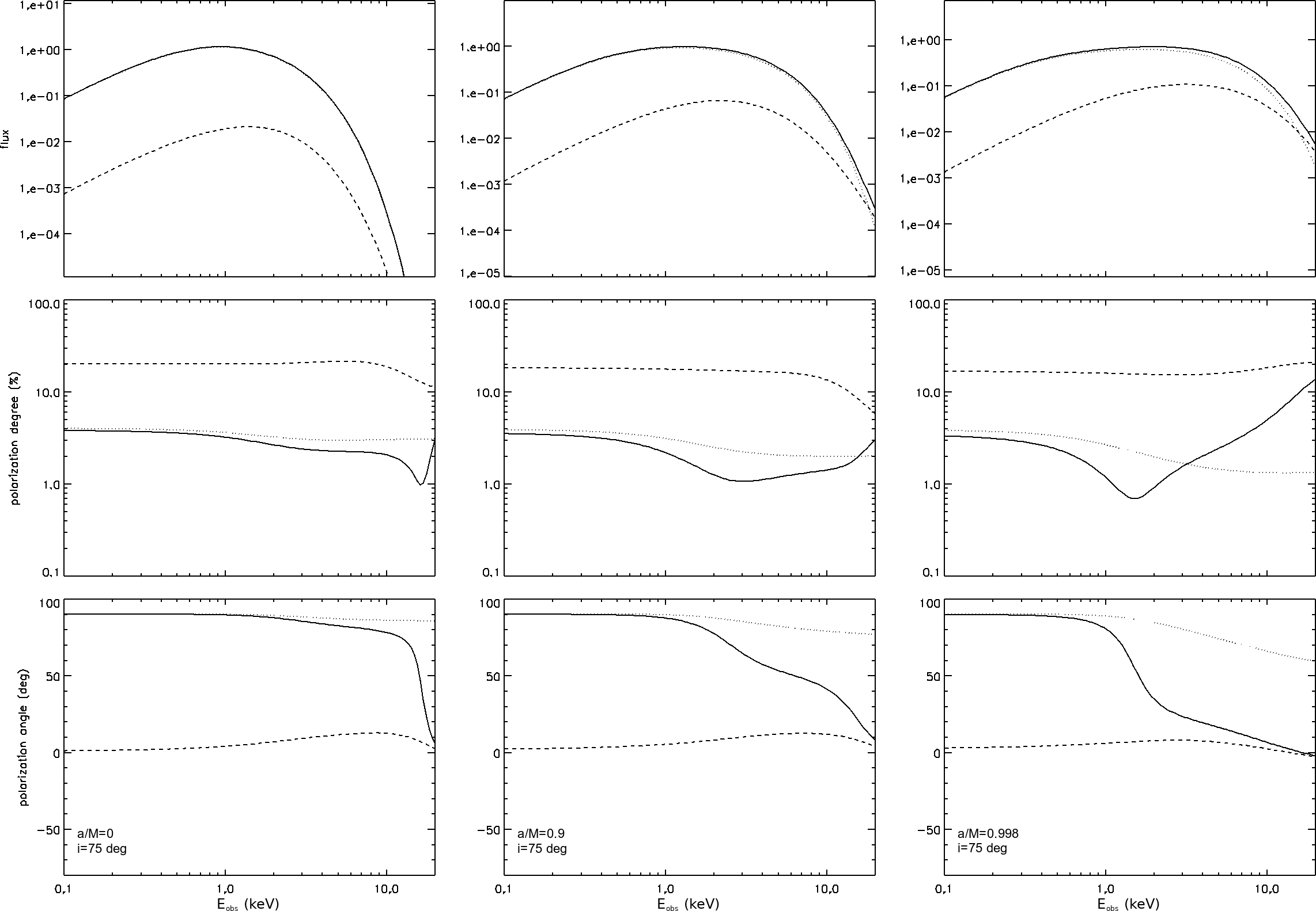
Figure 1: Spectrum (top row), polarization degree (middle row) and polarization angle (bottom row) plotted as functions of the photon energy at the observer for a BH mass $M=10\,M_{\odot}$ and spin $a=0$ (left-hand column), $0.9$ (middle column) and $0.998$ (right-hand column). The inclination angle $i$ between the observer’s line-of-sight and the disk symmetry axis is taken as $75^{\circ}$, while the BH mass accretion rate is chosen in such a way that the accretion luminosity is equal to $10\%$ of the Eddington limit. In particular $\dot{M}=2.45$ (for $a=0$), $0.90$ (for $a=0.9$) and $0.35$ (for $a=0.998$) in units of $10^{18}$ g s^-1 (see Table 1 of Krawczynski 2012). In each plot, the contributions of direct and returning photons alone are marked by dotted and dashed lines, respectively, while the joint contribution (direct $+$ returning radiation) is marked by solid lines.

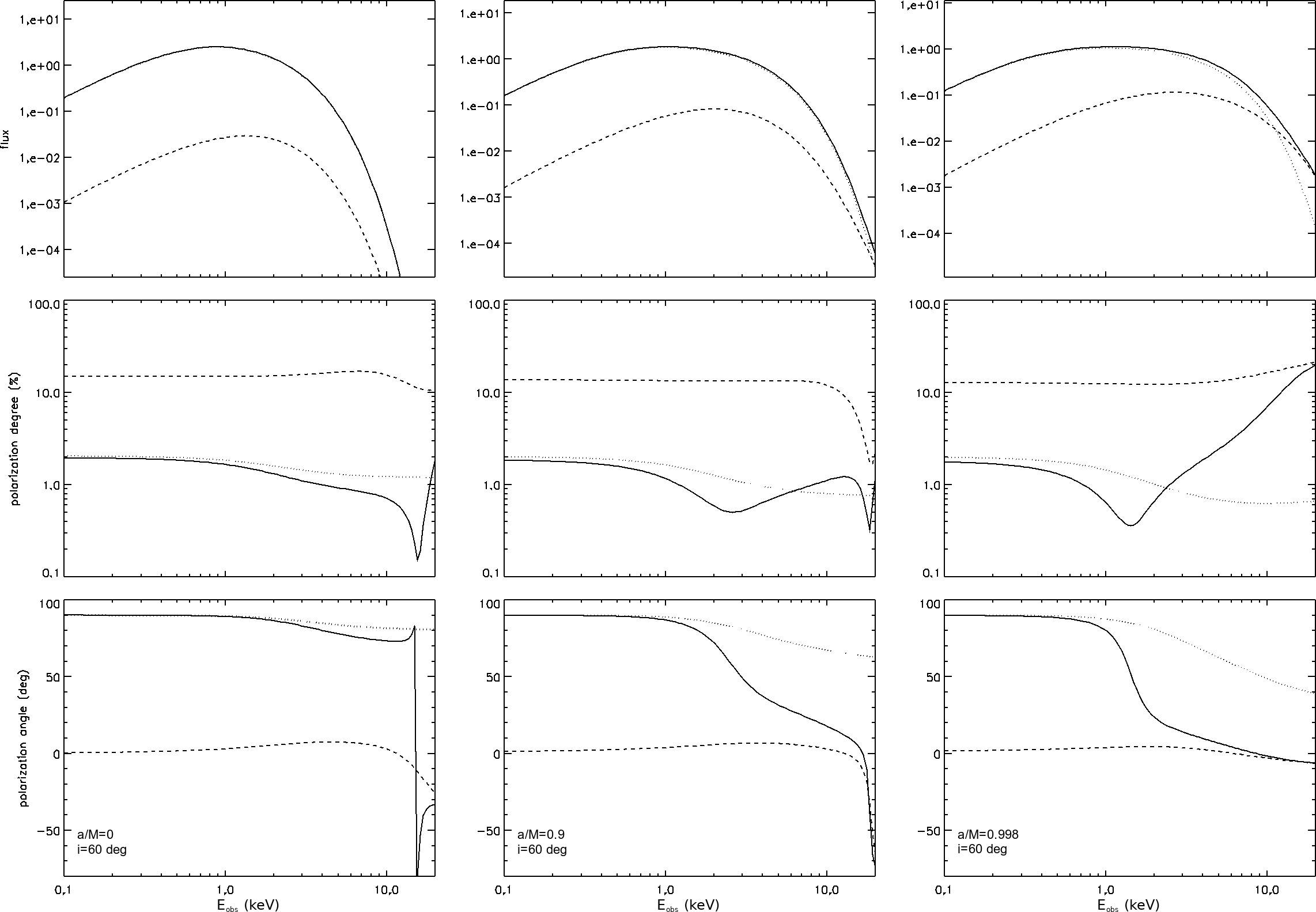
Figure 2: Same as in Figure 1 but for $i=60^{\circ}$.

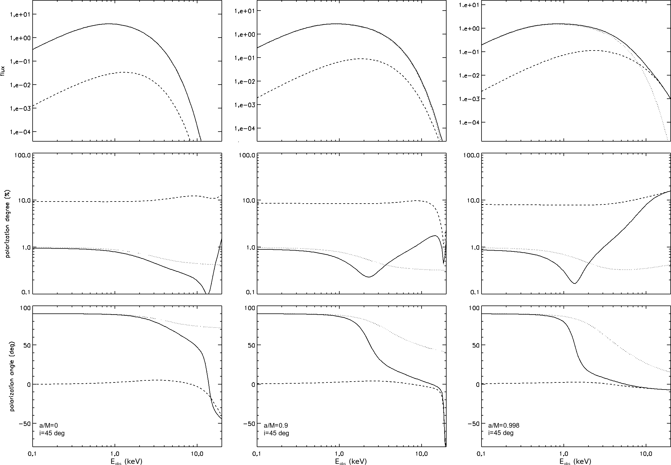
Figure 3: Same as in Figure 1 but for $i=45^{\circ}$.

For our calculations we used the kyn package Dovčiak (2004); Dovčiak et al. (2004a, b, c), which includes a set of different emission models built-in into xspec. The code exploits a fully relativistic, ray-tracing technique based on an observer-to-emitter approach. As photons emitted from the disk are assumed to follow a (multicolor) blackbody distribution, we resort to the model kynbb, which provides the spectral and polarization properties of radiation in the case of blackbody seed photons, following a Novikov-Thorne temperature profile with color correction (see section 2). However, since in its original version this model did not account for returning radiation, the first part of the present work consisted in expanding kyn, adding a specific routine to include the contributions of returning photons to spectra and polarization observables.

In order to briefly summarize how the code works, we remind here in broad terms the main features of kyn in dealing with the direct radiation case (we address the reader to Dovčiak et al., 2008, for a more in-depth view), before entering into details about the returning radiation section.

3.1 Direct radiation

The disk surface is sampled by a $(r,\phi)$ grid with $N_{\rm r}\times N_{\phi}$ points, where $r$ is the radial distance from the central BH and $\phi$ the azimuth with respect to a reference direction in the plane perpendicular to the disk axis. Once the observer inclination $\theta_{\mathrm{obs}}$ with respect to the disk normal is determined, the code traces back all the possible null geodesics which connect the observer to different points on the disk, followed by direct photons.

For each emission point of the disk surface grid, all the main quantities concerning the radiative transport are then provided in terms of photon number. In this respect, the photon flux $\Delta f_{\mathrm{obs}}$ observed at infinity in the energy bin $\langle E,E+\Delta E\rangle$ per unit solid angle can be written as

$$\Delta f_{\mathrm{obs}} =\int_{r_{\rm in}}^{r_{\rm out}}r\mathrm{d}r\int_{\phi^{\prime}}^{\phi^{\prime}+\Delta\phi^{\prime}}\mathrm{d}\phi\int_{E/g}^{(E+\Delta E)/g}Gf_{\mathrm{loc}}\mathrm{d}E_{\mathrm{loc}}\,,$$ (5)

where the subscript ‘loc’ refers to local quantities, $r_{\rm in}$ ($r_{\rm out}$) is the inner (outer) radius of the disk and $f_{\mathrm{loc}}$ is the local, energy-dependent photon number flux (see Dovčiak et al., 2008, for further details). The boundaries $\phi^{\prime}$ and $\Delta\phi^{\prime}$ of the azimuthal integration domain can be arbitrarily chosen in input (for integration over the entire disk surface it is $\phi^{\prime}=0$ and $\Delta\phi^{\prime}=2\pi$), as well as the values $E_{\mathrm{loc}}^{\rm min}$ and $E_{\mathrm{loc}}^{\rm max}$ which mark the range of variation of the local energy. Also $r_{\rm in}$ and $r_{\rm out}$ can be chosen as code inputs; in particular, the inner edge of the disk can be selected as coincident, larger or smaller than the innermost stable circular orbit. In the latter case, particles in the inner part of the disk are considered in free-fall towards the central BH, with the same energy and angular momentum they had at the ISCO. In the following, however, we assume $r_{\rm in}=r_{\rm ms}$.

As mentioned above, emitted photons are assumed to be polarized by electron scatterings which occur at the disk surface. In particular, in the diffusion limit ($\tau\gg 1$) the intrinsic polarization properties are given following the analytical expressions developed by Chandrasekhar (1960) for a geometrically-thin, optically-thick atmosphere with infinite optical depth. On the other hand, we also exploit the capability of the kyn package to explore configurations characterized by finite optical depths. In these cases, the intrinsic polarization pattern is numerically evaluated using the Monte Carlo code stokes, firstly developed by Goosmann & Gaskell (2007, see also and references therein for subsequent updates). It has been possible to verify a posteriori that all the configurations with $\tau\ga 5$ shall be regarded as equivalent to the $\tau=\infty$ case (see Figure 7; see also Dovčiak et al., 2008).

The code then calculates the local, energy-dependent Stokes parameters $\boldsymbol{s}_{\mathrm{loc}}^{\mathrm{dir}}=[i_{\mathrm{loc}}^{\mathrm{dir}},q_{\mathrm{loc}}^{\mathrm{dir}},u_{\mathrm{loc}}^{\mathrm{dir}}]$ and, once selected the polar angles $\theta$ and $\varphi$ the photon emission direction makes with the disk normal, it computes the integrated (energy-dependent) Stokes parameters at the observer as

$$i_{\mathrm{obs}} =\int{\rm d}S\,i_{\mathrm{loc}}^{\mathrm{dir}}(r,\phi)G$$

$$q_{\mathrm{obs}} =\int{\rm d}S\,[q_{\mathrm{loc}}^{\mathrm{dir}}(r,\phi)\cos(2\Psi)-u_{\mathrm{loc}}^{\mathrm{dir}}(r,\phi)\sin(2\Psi)]G$$

$$u_{\mathrm{obs}} =\int{\rm d}S\,[u_{\mathrm{loc}}^{\mathrm{dir}}(r,\phi)\cos(2\Psi)+q_{\mathrm{loc}}^{\mathrm{dir}}(r,\phi)\sin(2\Psi)]G\,.$$ (6)

In equations (3.1), $\Psi$ is the change in polarization angle (see equation 3) which accounts for the general relativistic effects that the photon polarization plane experiences as they propagate along each geodesic which connects the emission points to the observer. On the other hand, the transfer function $G=g^{2}l\cos\theta$, where $g=E_{\mathrm{obs}}/E_{\mathrm{loc}}$ is the energy shift and $l$ the lensing factor (i.e. the ratio between the flux tube cross sections at the observer and at the disk), accounts for the effects of strong gravity on the photon energies and directions along the same trajectories (see Dovčiak, 2004; Dovčiak et al., 2008, for more details). Finally, $\mathrm{d}S=r{\rm d}r{\rm d}\phi$ represents the surface integration element. As for equation (5), integration is extended over the radial range $r_{\rm in}<r<r_{\rm out}$ and the azimuthal range $\phi^{\prime}<\phi<\phi^{\prime}+\Delta\phi^{\prime}$. Polarization observables, i.e. the polarization degree $P$ and angle $\chi$, are eventually obtained as

$$P =\frac{\sqrt{q^{2}+u^{2}}}{i}$$

$$\chi =\frac{1}{2}\arctan\left(\frac{u}{q}\right)\,,$$ (7)

where $i$, $q$ and $u$ should be substituted with the expressions given in equations (3.1).

3.2 Returning radiation

In order to include the contributions of returning radiation inside kyn, we use the c++ code selfirr, based on the ray-tracing sim5 package Bursa (2017), that computes all the possible null geodesics connecting two different points on the disk surface, along which returning photons move.

Returning photons are considered to collide with the disk along a general direction $(\bar{\theta}_{\rm i},\bar{\varphi}_{\rm i})$, with $\bar{\theta}_{\rm i}$ and $\bar{\varphi}_{\rm i}$ the polar angles with respect to the disk normal. The disk surface is therefore divided into $\bar{N}_{\rm r}$ incidence patches, each characterized by the radial distance $\bar{r}_{\rm i}$ of their centers from the BH, while all the possible incidence directions are in turn sampled through a discrete $\bar{N}_{\theta}\times\bar{N}_{\varphi}$ angular mesh. An orthonormal tetrad $e_{(a)}^{\mu}$ is then attached to the disk fluid at each radius, following Appendix A.2 of Zhang, Dovčiak & Bursa (2019); in this way, in the tetrad frame comoving with the disk fluid, the wave vector associated to each returning photon can be written as

$$k^{(a)} =\{1,\sin\bar{\theta}_{\rm i}\cos\bar{\varphi}_{\rm i},\cos\bar{\theta}_{\rm i},\sin\bar{\theta}_{\rm i}\sin\bar{\varphi}_{\rm i}\}$$ (8)

or, by switching to the Boyer-Lindquist coordinate frame, as

$$k^{\mu} =e^{\mu}_{(a)}k^{(a)}\,.$$ (9)

Following Carter (1968) and Li et al. (2005), the code exploits $k^{\mu}$ to evaluate the constants of motion which characterize each photon and determine whether the photon trajectory actually connects the incidence point to another point of the disk surface or not. If yes, the code solves the geodesic equation for the radius $\bar{r}_{\rm e}$ of the point at which the photon was emitted from the disk and calculate the angles $\bar{\theta}_{\rm e}$ and $\bar{\varphi}_{\rm e}$ which identify the emission direction with respect to the disk normal (see Li et al., 2005). This also allows to compute the value of the energy shift

$$\bar{g} =\frac{E_{\rm i}}{E_{\rm e}}=\frac{k_{\mu{\rm i}}U^{\mu}_{\rm i}}{k_{\mu{\rm e}}U^{\mu}_{\rm e}}$$ (10)

which accounts for general relativistic effects along each returning geodesic, with $U_{\rm i}^{\mu}$ ($U_{\rm e}^{\mu}$) the four-velocity of the disk fluid at the incidence (emission) point. The angle $\bar{\Psi}(\bar{r}_{\rm i},\bar{\theta}_{\rm i},\bar{\varphi}_{\rm i})$ by which the photon polarization plane is rotated while returning to the disk is eventually provided. This is done again by evaluating the Walker-Penrose constant (as mentioned in section 2), following equations B46–B47 of Li et al. (2009).

The code returns in output a fits file to be read by kyn. This contains, for each value of $\bar{r}_{\rm i}$, the values of the incidence angles $(\bar{\theta}_{\rm i},\bar{\varphi}_{\rm i})$, the radial distance $\bar{r}_{\rm e}$ of the starting point and the emission angles $(\bar{\theta}_{\rm e},\bar{\varphi}_{\rm e})$, the energy shift $\bar{g}$, the solid angle $\Delta\bar{\Omega}_{\rm i}$ of the pixel with incidence angles $\bar{\theta}_{\rm i}$ and $\bar{\varphi}_{\rm i}$ and the change in polarization angle $\bar{\Psi}$. Input parameters of each selfirr run are, instead, the specific BH spin $a$, the disk outer radius $r_{\rm out}$ and the number of points $\bar{N}_{\rm r}$, $\bar{N}_{\theta}$ and $\bar{N}_{\varphi}$ of the different discrete grids introduced above. For the sake of convenience, we chose $r_{\rm out}$ as coincident to the disk outer radius set in the calculations of the direct radiation contributions (see section §3.1), much in the same way as the numbers of radial grid points $\bar{N}_{\rm r}$ and $N_{\rm r}$. This ensures that the radial grids which sample the disk surface in the two codes kyn and selfirr are the same, so that the contributions of direct and returning radiation can be simply summed together at each point of this unique surface grid without any additional numerical manipulation (see equation 3.2).

As in the case of the direct radiation, the Stokes parameters $\boldsymbol{\bar{s}}_{\rm e}=[\bar{i}_{\rm e},\bar{q}_{\rm e},\bar{u}_{\rm e}]$ of returning photons at their emission are given following the Chandrasekhar’s (1960) formulae or, alternatively, using the tables obtained from the Monte Carlo code stokes (see §3.1), according to their emission radius $\bar{r}_{\rm e}$ and direction $(\bar{\theta}_{\rm e},\bar{\varphi}_{\rm e})$. Returning photons are then reflected at the disk surface. In order to evaluate the Stokes vectors $\boldsymbol{\bar{s}}_{\mathrm{refl}}(P_{\mathrm{refl}},\chi_{\mathrm{refl}})=[\bar{i}_{\mathrm{refl}},\bar{q}_{\mathrm{refl}},\bar{u}_{\mathrm{refl}}]$, where $P_{\mathrm{refl}}$ and $\chi_{\mathrm{refl}}$ denote the polarization degree and angle after reflection, we use the Chandrasekhar’s (1960) formulae for diffuse reflection. First, the code computes the Stokes parameters for three distinct states of polarization, corresponding to unpolarized light ($P_{\mathrm{refl}}=0$) and fully polarized radiation ($P_{\mathrm{refl}}=1$) with $\chi_{\mathrm{refl}}=0$ and $45^{\circ}$, respectively (see Appendix A for more details). Then it reconstructs the Stokes vector for a generic state of polarization through the decomposition

$$\boldsymbol{\bar{s}}_{\mathrm{refl}}(P_{\mathrm{refl}}, \chi_{\mathrm{refl}})=\boldsymbol{\bar{s}}_{\mathrm{refl}}(0,-)$$

$$\,\,\,\,\,+P_{\rm e}\{[\boldsymbol{\bar{s}}_{\mathrm{refl}}(1,0)-\boldsymbol{\bar{s}}_{\mathrm{refl}}(0,-)]\cos[2(\chi_{\rm e}+\bar{\Psi})]$$

$$\,\,\,\,\,+[\boldsymbol{\bar{s}}_{\mathrm{refl}}(1,\pi/4)-\boldsymbol{\bar{s}}_{\mathrm{refl}}(0,-)]\sin[2(\chi_{\rm e}+\bar{\Psi})]\}\,,$$ (11)

which follows from the definition (3.1) of $P$ and $\chi$ in terms of the Stokes parameters, with $P_{\rm e}$ and $\chi_{\rm e}$ the polarization degree and angle at the emission point.

All the contributions coming from the different incidence directions at each incidence point are finally summed together, obtaining the contribution to the (energy-dependent) local Stokes parameters for returning photons,

$$i_{\mathrm{loc}}^{\mathrm{ret}}(\bar{r}_{\rm i}) =\sum_{\bar{\theta}_{\rm i},\bar{\varphi}_{\rm i}}\bar{i}_{\mathrm{refl}}(\bar{r}_{\rm i},\bar{\theta}_{\rm i},\bar{\varphi}_{\rm i})\bar{g}^{2}(\bar{r}_{\rm i},\bar{\theta}_{\rm i},\bar{\varphi}_{\rm i})\bar{\mu}_{\rm i}\Delta\bar{\Omega}_{\rm i}$$

$$q_{\mathrm{loc}}^{\mathrm{ret}}(\bar{r}_{\rm i}) =\sum_{\bar{\theta}_{\rm i},\bar{\varphi}_{\rm i}}\bar{q}_{\mathrm{refl}}(\bar{r}_{\rm i},\bar{\theta}_{\rm i},\bar{\varphi}_{\rm i})\bar{g}^{2}(\bar{r}_{\rm i},\bar{\theta}_{\rm i},\bar{\varphi}_{\rm i})\bar{\mu}_{\rm i}\Delta\bar{\Omega}_{\rm i}$$

$$u_{\mathrm{loc}}^{\mathrm{ret}}(\bar{r}_{\rm i}) =\sum_{\bar{\theta}_{\rm i},\bar{\varphi}_{\rm i}}\bar{u}_{\mathrm{refl}}(\bar{r}_{\rm i},\bar{\theta}_{\rm i},\bar{\varphi}_{\rm i})\bar{g}^{2}(\bar{r}_{\rm i},\bar{\theta}_{\rm i},\bar{\varphi}_{\rm i})\bar{\mu}_{\rm i}\Delta\bar{\Omega}_{\rm i}\,,$$ (12)

where $\bar{\mu}_{\rm i}=\cos{\bar{\theta}_{\rm i}}$. The integrated Stokes parameters at the observer are computed following the same procedure described in section 3.1 for direct radiation; in particular, equations (3.1) become,

$$i_{\mathrm{obs}} =\int{\rm d}S\,i_{\mathrm{loc}}(r,\phi)G$$

$$q_{\mathrm{obs}} =\int{\rm d}S\,[q_{\mathrm{loc}}(r,\phi)\cos(2\Psi)-u_{\mathrm{loc}}(r,\phi)\sin(2\Psi)]G$$

$$u_{\mathrm{obs}} =\int{\rm d}S\,[u_{\mathrm{loc}}(r,\phi)\cos(2\Psi)+q_{\mathrm{loc}}(r,\phi)\sin(2\Psi)]G\,,$$ (13)

where, in this case,

$$i_{\mathrm{loc}}(r,\phi) =i_{\mathrm{loc}}^{\mathrm{dir}}(r,\phi)+i_{\mathrm{loc}}^{\mathrm{ret}}(r)$$

$$q_{\mathrm{loc}}(r,\phi) =q_{\mathrm{loc}}^{\mathrm{dir}}(r,\phi)+q_{\mathrm{loc}}^{\mathrm{ret}}(r)$$

$$u_{\mathrm{loc}}(r,\phi) =u_{\mathrm{loc}}^{\mathrm{dir}}(r,\phi)+u_{\mathrm{loc}}^{\mathrm{ret}}(r)\,.$$ (14)

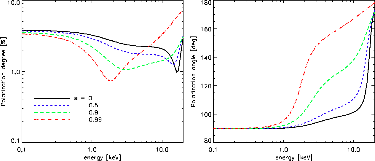
Figure 4: Polarization degree (left) and polarization angle⁹ (right), plotted as functions of the photon energy at the observer, for $i=75^{\circ}$ and different values of the BH spin: $a=0$ (solid black), $0.5$ (dashed blue), $0.9$ (long-dashed green) and $0.99$ (dash-dotted red). Input parameters are taken as in Krawczynski (2012, see his Table 1).

The output of a typical kyn run consists in a table containing the values of the integrated Stokes parameters $\boldsymbol{s}_{\mathrm{obs}}=[i_{\mathrm{obs}},q_{\mathrm{obs}},u_{\mathrm{obs}}]$ as functions of the photon energy. This also allows to obtain the energy-dependent polarization observables $P_{\mathrm{obs}}$ and $\chi_{\mathrm{obs}}$, by substituting equations (3.2) into equations (3.1). Alternatively, spectra and polarization properties can be also obtained for either direct or returning radiation contributions separately, by omitting in equations (3.2) the returning or the direct terms, respectively.

4 Results

With the purpose of an immediate comparison of our results with previous works (in particular Schnittman & Krolik, 2009; Krawczynski, 2012), and in order to ensure that our code is well implemented, we initially assume a 100% albedo prescription, i.e. all the photons which return to the disk are considered to be reflected towards infinity. As an extension of the above-mentioned works, we also obtain results for finite optical depths of the pure-electron disk atmosphere. Finally, we discuss how the spectral and polarization properties of the collected radiation can be modified assuming more realistic albedo profiles.

4.1 Case of 100% disk albedo

We firstly remark that, contrary to our ray-tracing code, which is based on an observer-to-emitter approach, those exploited by Schnittman & Krolik (2009) and Krawczynski (2012), to which we refer in the following as benchmarks, rely on an emitter-to-observer paradigm (see Schnittman & Krolik, 2013, for more details). In the light of this, a comparison with their results becomes even more significant, since it also allows to check if our code gives similar expectations to those already presented in literature and obtained using different techniques.

In order to make our simulations comparable with those presented by both Schnittman & Krolik (2009) and Krawczynski (2012), we assumed a central BH with mass $M=10\,M_{\odot}$ and accreting material at a rate $\dot{M}\approx 10\%$ of the Eddington limit $\dot{M}_{\rm Edd}$ (correctly accounting for the change in efficiency for different values of the BH spin $a$). Moreover, we chose a constant hardening factor $f_{\rm col}=1.8$. The energy domain is characterized by a 200-point grid between $0.01$ and $50$ keV, while the disk surface has been sampled through a grid characterized by $N_{\rm r}=500$ radial bins, logaritmically-spaced between $r_{\rm ms}$ and $r_{\rm out}=100\,r_{\rm g}$, and $N_{\phi}=180$ azimuthal zones. We then associated to each point $\bar{N}_{\theta}\times\bar{N}_{\phi}=100\times 100$ incidence directions for what concerns returning radiation, i.e. $10^{4}$ rays are traced per radius and azimuth. Finally, the polarization properties of photons at their emission are derived using Chandrasekhar’s (1960) formulae, considering an infinite optical depth $\tau$ for the atmospheric layer that is assumed to cover the disk surface.

Figures 1–3 show the behaviors of spectra (energy flux of the Stokes parameter $i$) and polarization observables ($P_{\mathrm{obs}}$ and $\chi_{\mathrm{obs}}$) as functions of the photon energy at the observer, considering the line-of-sight inclined by $75^{\circ}$, $60^{\circ}$ and $45^{\circ}$ with respect to the disk symmetry axis and for three different values of the BH spin: $a=0$, $0.9$ and $0.998$. In all the plots the contributions of direct and returning radiation alone (dotted and dashed lines, respectively) can be distinguished from the joint contribution (solid lines) obtained by summing the two, as illustrated in §3.2.

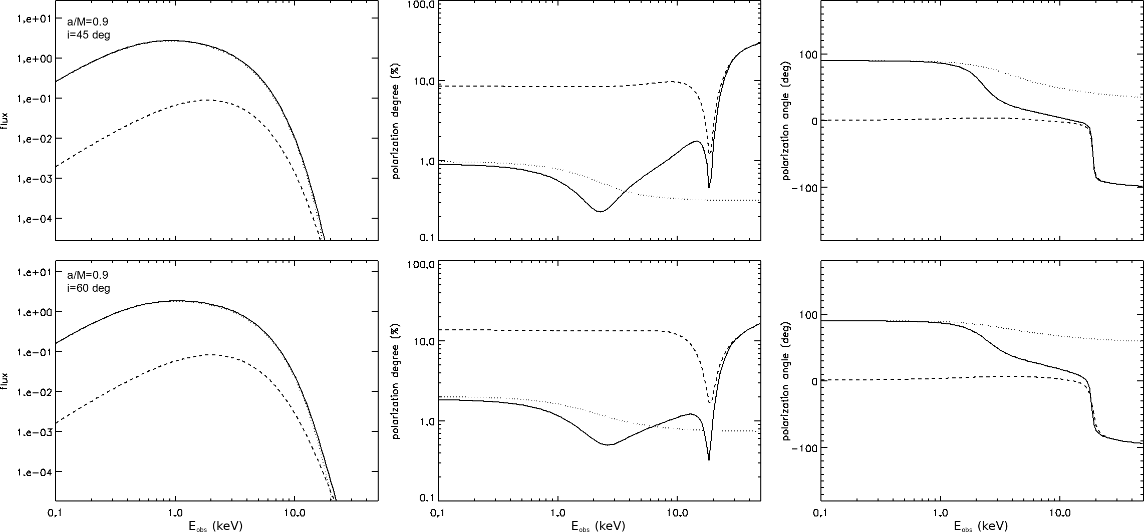
Figure 5: Spectrum (left-hand column), polarization degree (middle column) and polarization angle (right-hand column), plotted as functions of the photon energy at the observer, for $a=0.9$ and $i=45^{\circ}$ (top row) and $i=60^{\circ}$ (bottom row). Details as in Figures 1–3.

As a quick comparison with the plots reported in their Figures 4–6 clearly shows, our results turn out to be in general compatible with those presented by Schnittman & Krolik (2009). In particular, as expected for large optical depths (see e.g. Dovčiak et al., 2008), direct radiation turns out to be polarized perpendicularly to the disk symmetry axis at lower energies, i.e. the polarization angle associated to the direct radiation component $\chi^{\mathrm{dir}}_{\mathrm{obs}}$ is about $90^{\circ}$, while it slowly decreases at higher energies ($\ga 2$ keV) under the effect of the polarization plane rotation (see section 2). This can be explained looking at the behavior of the disk temperature profile as a function of the radial distance from the center (see e.g. Figure 10). Low-energy photons are emitted from the external regions of the disk, where the temperature is lower and strong gravity is less important, whereas high-energy ones are emitted closer to the BH, where the temperature is higher and photon polarization is mostly affected by general relativistic effects. On the other hand, returning photons appear to be mostly polarized parallel to the disk axis ($\chi^{\mathrm{ret}}_{\mathrm{obs}}=0^{\circ}$), although also in this case the polarization angle slightly declines above $10$ keV due to general relativistic effects (even if by a smaller amount than in the direct radiation case). Looking at the joint contribution (direct $+$ returning radiation), a transition between the two regimes can be observed. In particular, the total polarization angle $\chi_{\mathrm{obs}}$ follows the curve of direct radiation alone as long as the fraction of returning photons becomes comparable to that of direct ones (see the spectra in the top rows), while it swings by $90^{\circ}$ at higher frequencies. The energy at which this transition occurs turns out to be smaller the larger the BH spin, that is mainly due to the choice of considering $r_{\rm in}$ as coincident to $r_{\rm ms}$. In fact, the innermost stable circular orbit lies at a larger distance from the center for a non-rotating BH, while it approaches the horizon as $a$ increases. As a consequence, for $a=0$ returning photons start to dominate only at very high energies ($\ga 10$ keV), once the spectrum of direct photons has sufficiently declined, while for $a=0.9$ and $0.998$ the transition occurs already at $E_{\mathrm{obs}}\ga 1$ or $2$ keV, since more high-energy returning photons populate the spectral tail at those energies.

The trend of the polarization degree can be explained in a rather similar way. Having assumed that the radiative transfer in the atmospheric layer which covers the disk surface is dominated by (Thomson) electron scatterings with $\tau\rightarrow\infty$, direct radiation turns out to be quite mildly polarized, with $0.3\%\leq P^{\mathrm{dir}}_{\mathrm{obs}}\leq 3\%$. Returning radiation, instead, is much more polarized, with in general $8\%\leq P^{\mathrm{ret}}_{\mathrm{obs}}\leq 20\%$. As in the polarization angle plots, a transition between the direct and returning radiation regimes can be observed when contributions are summed together. While the $P^{\rm tot}_{\mathrm{obs}}$ essentially follows the behavior of direct radiation below $\sim 1$ keV, it attains a minimum in correspondence of the polarization angle swing described above, and then it approaches the returning radiation trend at higher energies.

For the sake of a further comparison with works previously published in literature, we also produced supplementary plots (see Figure 4) for the energy-dependent polarization degree and angle, to be compared with those reported by Krawczynski (2012), who showed expectations for different kinds of space-time metrics. Also in this case, limiting our analysis to the case of a Kerr BH (see his Figure 5), an overall good agreement should be noted between the different simulations performed for the polarization observables behaviors, obtained for $a=0$, $0.5$, $0.9$ and $0.99$ and $i=75^{\circ}$.

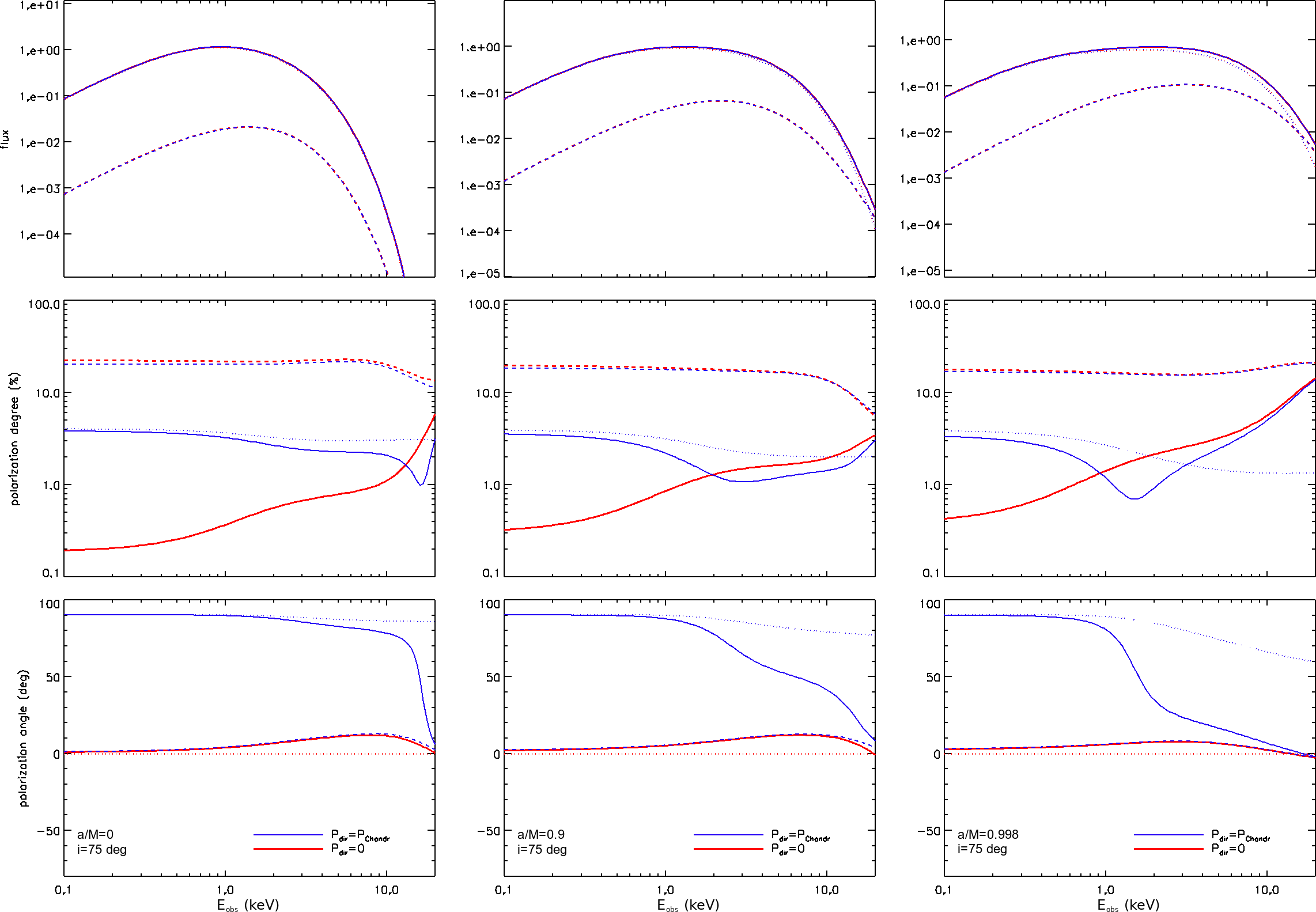
Figure 6: Spectrum (top row), polarization degree (middle row) and polarization angle (bottom row) behaviors, plotted as functions of the photon energy at the observer, for direct radiation polarized according to Chandrasekhar’s (1960) formulae ($P_{\mathrm{dir}}=P_{\rm Chandr}$, blue lines) and assuming that emitted radiation is unpolarized ($P_{\mathrm{dir}}=0$, red lines). Parameter values and line styles are taken as in Figure 1 (see also text for more details).

Some differences with respect to the results reported in Schnittman & Krolik (2009), however, are present when the case of $a=0.9$ is considered. This is already visible in the middle column of Figures 2 and 3, where a second minimum in the (joint) polarization degree behavior appears in addition to that just discussed above, related to the transition from the direct to the returning radiation regimes. This second minimum occurs in connection with a steep decrease in the polarization angle of the returning radiation component, at an energy $\sim 20$ keV. To better investigate this feature, we report in Figure 5 the same plots (for $a=0.9$ and $i=45^{\circ},\,60^{\circ}$), but extending the energy range on the horizontal axis up to $50$ keV. As it can be clearly seen in the right panels, for these values of the input parameters the polarization direction of returning photons seems change from parallel ($\chi_{\rm obs}^{\rm ret}=0^{\circ}$) to perpendicular ($\chi_{\rm obs}^{\rm ret}=-90^{\circ}$) to the disk symmetry axis at very high energies. We checked a posteriori that this behavior is still present also increasing the resolution of the energy, radial and angular grids; this led us to the conclusion that this particular feature may not be a numerical artifact.

In order to understand the physical mechanism responsible for this behavior, we looked in more details on the values of the polarization degree and angle of the reflected radiation as functions of the position on the disk surface. We found that an additional critical point (as discussed in Dovčiak et al., 2008, 2011) appears close to the BH for the largest spin values and the highest inclinations, around which the polarization angle attains all possible values. The existence of this critical point is due to the complex dependence of Chandrasekhar’s (1960) diffuse reflection formulae (in the multi-scattering approximation) on the incidence and emission scattering angles, as well as on the photon polarization angle at the reflection point. In most cases, the rather small region around the critical point does not affect sizeably the overall Stokes parameter distributions. High-energy photons come from a well-defined, “hot” region of the disk close to the ISCO where the temperature is higher. The Doppler shift has to be important, which means that it is on the approaching side of the disk, but at the same time the gravitational redshift is not too large, which means that it is not too close to the BH horizon. If the critical point lies far away from this peculiar region, one does not see any abrupt change in the polarization properties at high energies, since the Stokes parameters do not change too much in the vicinity of this zone. The situation is different when the critical point is close to this hot region. In fact, while the Stokes parameters at low-energies are integrated over a large area of the disk surface, those at high energies come from a localized region and this results in different polarization patterns. In particular, in our case it turns out that the critical point is close enough to the hot region only for not too high spin values ($a=0.9$). For $a\simeq 0$ the critical point does not even exist (i.e. it would lie below the ISCO), while it moves closer to the horizon, and on the other side of the BH wrt the hot region, for very high spins ($a=0.998$).

However, as it can be noted from the spectra reported in the left panels of Figure 5, at such high energies ($\ga 20$ keV) the photon flux is dramatically smaller than at the spectral peak (by almost $5$ orders of magnitude). This certainly reduces the overall importance of catching such a behavior in the polarization observable trends, since polarimetric techniques (especially at X-ray energies) would suffer for the extremely low number of photons expected.

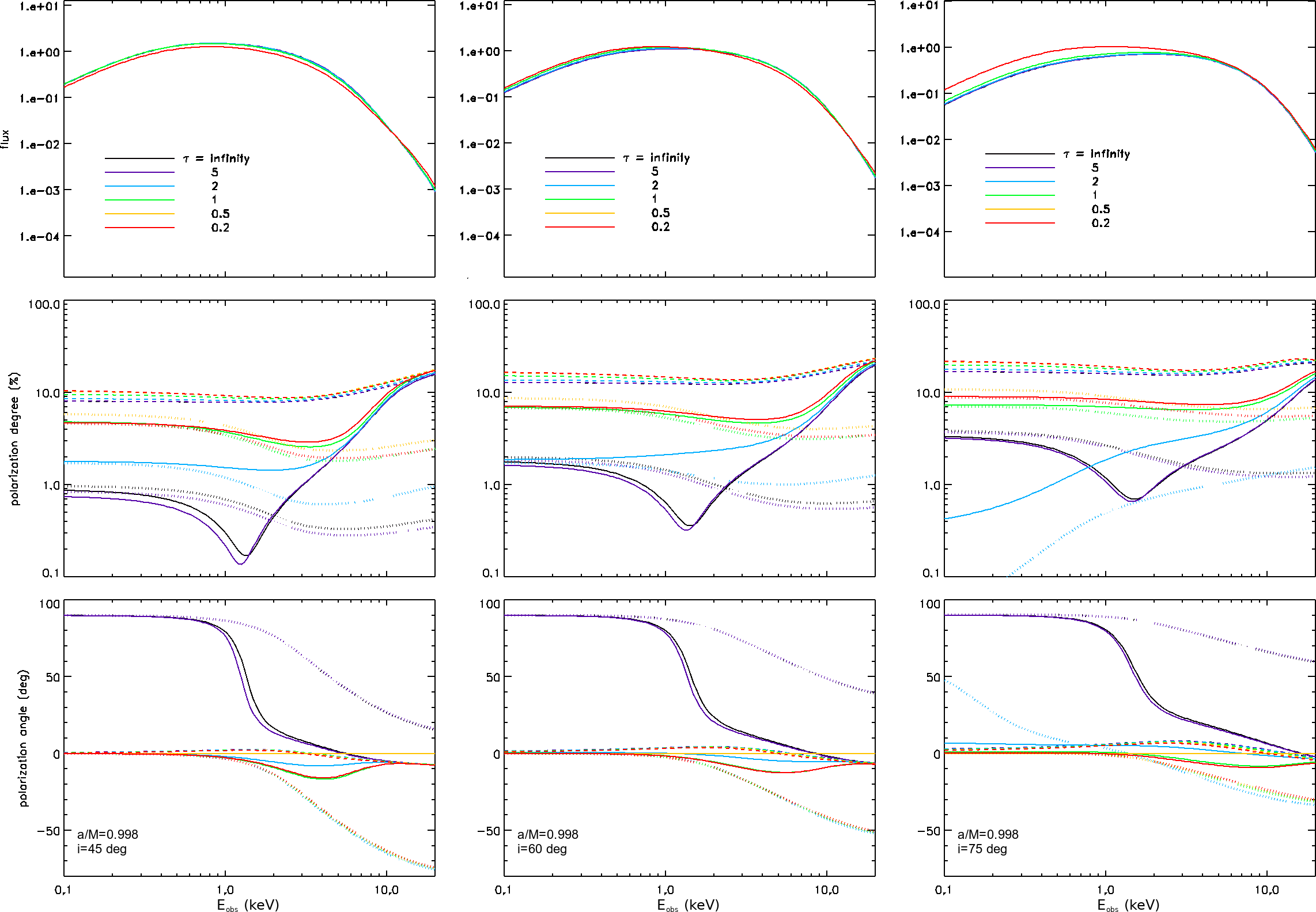
Figure 7: Spectrum (top row), polarization degree (middle row) and polarization angle (bottom row) plotted as functions of the photon energy at the observer for $a=0.998$ and $i=45^{\circ}$ (left-hand column), $60^{\circ}$ (middle column) and $75^{\circ}$ (right-hand column), and for different value of the atmosphere optical depth: $\tau\rightarrow\infty$ (black), $5$ (purple), $2$ (cyan), $1$ (green), $0.5$ (orange) and $0.2$ (red). Details as in Figure 1 (for the sake of convenience, the separate direct and returning radiation contributions are shown in the polarization observable plots only).

In order to better understand how returning radiation influences the polarization properties of collected photons at infinity and to disentangle its effects from those of direct radiation, we performed analogous simulations assuming that photons are emitted from the disk as unpolarized (i.e. we artificially imposed $P^{\mathrm{dir}}_{\mathrm{loc}}=0$). Illustrative plots are shown in Figure 6 for $a=0$, $0.9$ and $0.998$ and $i=75^{\circ}$ (red lines), while the corresponding ones, i.e. for direct radiation polarized according to Chandrasekhar’s (1960) formulae (see Figure 1), are reported in blue for ease of comparison. As it can be easily observed in the polarization fraction plots (middle row), returning photons are practically polarized at the same degree in the two cases, with only slight differences $\la 1\%$ (which are larger for smaller BH spins). This shows that the polarization properties of returning radiation do not actually depend on the intrinsic polarization state of photons. Rather, polarization of returning photons rises essentially upon reflection at the disk surface (see Appendix A). Moreover, assuming that photons are unpolarized at the emission, the collected radiation turns out to be polarized along the disk axis over the entire energy range, with no transitions (red solid lines in the bottom row of Figure 6). This allows the total polarization degree to monotonically increase with the photon energy (red solid lines in the middle row), up to reach a modest degree of polarization at sufficiently high energies which can also exceed that expected when direct photon polarization is properly accounted for.

4.2 Exploring different optical depths

While the results discussed in the previous subsection have been obtained assuming an infinite optical depth $\tau$ for the scattering atmosphere on the top of the blackbody-emitting disk, here we investigate how the spectral and polarization properties of the collected radiation can be influenced by changing $\tau$. We remind, in this regard, that special tables generated through the Monte Carlo code stokes are used to evaluate the photon Stokes parameters when finite values of $\tau$ are considered, at variance with the case of infinite $\tau$, for which the photon polarization state can be obtained using the analytical formulae by Chandrasekhar (1960). Figure 7 shows the behaviors of spectra and polarization observables at infinity, plotted as functions of the photon energy, for a maximally-rotating BH ($a=0.998$) and different inclinations of the observer’s line-of-sight. Results for $\tau=5$, $2$, $1$, $0.5$ and $0.2$ are provided, together with the case of $\tau\rightarrow\infty$ (black lines), already discussed in §4.1.

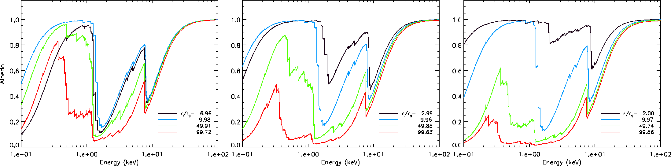
Figure 8: Albedo profile as a function of the local photon energy $E_{\mathrm{loc}}$ obtained from cloudy according to the temperature and density profiles given by equations (2) and (47), respectively, with $N_{\rm H}=10^{24}$ cm^-2, for $a=0$ (left), $0.9$ (center) and $0.998$ (right). Different colors refer to different radial distances from the center (see the plot legend for the color code). Values of mass and accretion rates are taken as in Figure 1.

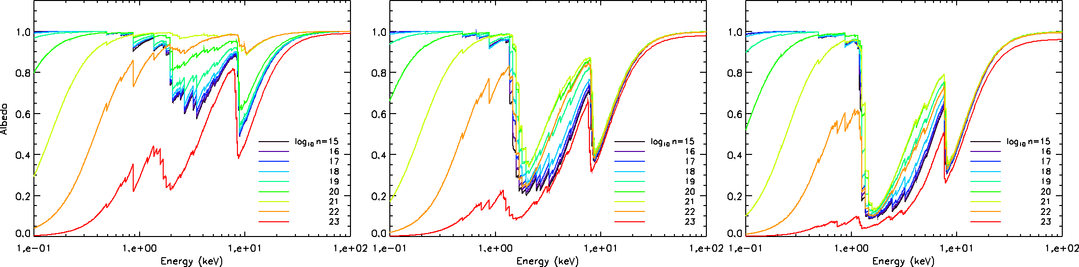
Figure 9: Albedo profile as a function of the local photon energy $E_{\mathrm{loc}}$ obtained from different runs of cloudy according to the temperature profile given by equation (2), for $a=0.998$ and $r/r_{\rm g}\sim 2$ (left), $5$ (center) and $10$ (right). The total hydrogen density is considered as constant for each run, with $\log n(\rm H)=15$–$23$, step $1$, in units of cm^-3 (see the plot legend for the color code). $N_{\rm H}=10^{24}$ cm^-2, while the values of mass and accretion rates are as in Figure 1.

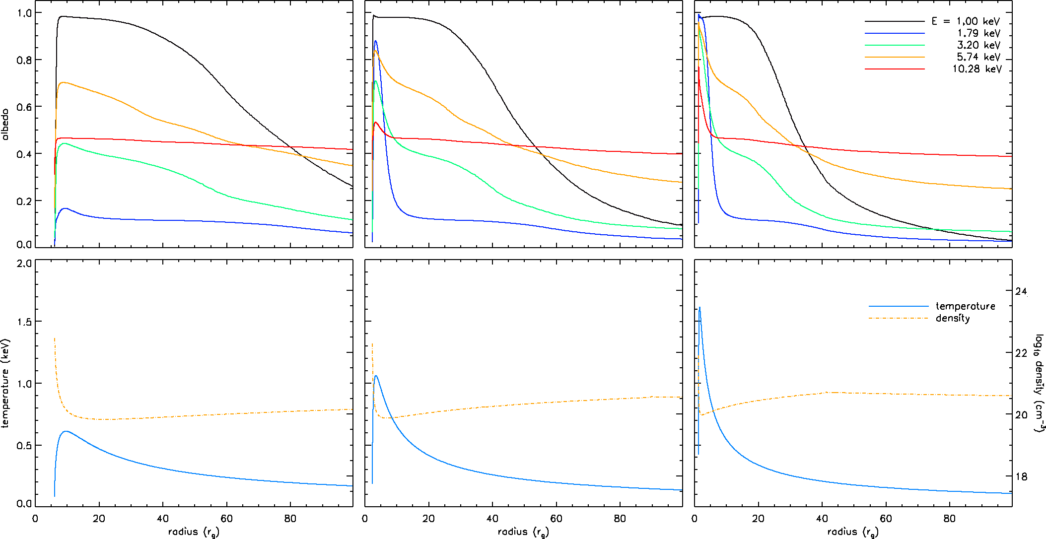
Figure 10: Top row: albedo profile as a function of the radial distance $r$, obtained for different local energies in the $1$–$10$ keV range (see the plot legend for the color code), in the cases of $a=0$ (left), $0.9$ (center) and $0.998$ (right). Bottom row: temperature (blue, solid line) and density (orange, dashed line) radial profiles described by equations (2) and (47), respectively, for $a=0$ and $\dot{M}=24.5\times 10^{17}$ g s^-1 (left), $a=0.9$ and $\dot{M}=9\times 10^{17}$ g s^-1 (middle), $a=0.998$ and $\dot{M}=3.5\times 10^{17}$ g s^-1 (right). In all the plots a BH mass of $M=10\,M_{\odot}$ has been assumed.

Spectra (top row) turn out to be quite unaffected by changing the optical depth; an appreciable, albeit small, spread is visible only in the case of $i=75^{\circ}$, mainly due to the different emission directionality of the primary emission. However, the most considerable changes appear in the polarization observables of the direct radiation components (see dotted lines in the middle and bottom rows). If on one hand both the polarization degree and angle behaviors for $\tau=5$ (purple) resemble those obtained for an infinite optical depth (black), on the other hand quite different trends are displayed for the other cases referred. More in detail, the polarization angle (bottom row) turns out to assume a value close to $0$ over the entire energy range for $\tau\la 2$. This can be explained by the fact, already noticed by Dovčiak et al. (2008, see their Figure 1), that a transition occurs at $\tau\sim 2$ in the orientation of the polarization vectors for direct photons: polarization is perpendicular to the projected disk symmetry axis ($\chi^{\mathrm{dir}}_{\mathrm{obs}}=90^{\circ}$) at high values of $\tau$, while it becomes parallel ($\chi^{\mathrm{dir}}_{\mathrm{obs}}=0^{\circ}$, as for returning radiation) at lower optical depths. An overview of the three plots, reported in the bottom row of Figure 7, shows that this transition also depends on the inclination angle. In fact, focussing on the case of $\tau=2$ (cyan), $\chi^{\mathrm{dir}}_{\mathrm{obs}}\sim 0^{\circ}$ for $i=45^{\circ}$ and $60^{\circ}$ at low energies (it decreases towards negative values at higher energies due to general relativistic effects, see §4.1), while it becomes significantly larger than $0$ only for $i=75^{\circ}$. By contrast, the polarization angle of returning radiation only (dashed lines) remains basically unchanged with respect to the case of $\tau\rightarrow\infty$ also when a finite optical depth is considered. This naturally follows from the fact that the polarization properties of returning photons barely depend on the mechanisms that polarize photons at their emission, being essentially determined by reflection (as discussed above). As a result, the polarization angle related to the joint contribution (direct $+$ returning radiation, solid lines) shows the typical swing due to the transition between the two regimes (see Figures 1–3) only for $\tau=5$ and $\tau\rightarrow\infty$, while no transition occurs for lower optical depths.

Looking at the polarization fraction plots (middle row) one can observe a behavior with optical depth and inclination angle similar to that just discussed for the polarization angle. In particular, the polarization degree for direct radiation ($P^{\mathrm{dir}}_{\mathrm{obs}}$) at $\tau=2$ and $i=75^{\circ}$ attains very low values ($<0.1\%$) at low energies, before to increase at higher energies up to a value not much larger than $1\%$. On the contrary, for lower inclination angles ($i=45^{\circ}$ and $60^{\circ}$) $P^{\mathrm{dir}}_{\mathrm{obs}}$ maintains a value of the order of few precents in the entire energy range. For even smaller values of the optical depth, the polarization fraction of the direct component attains generally higher values, regardless of the observer’s inclination. This is mainly due to the increase in polarization fraction that direct photons undergoes by decreasing $\tau$, as again confirmed by the results discussed in Dovčiak et al. (2008). On the other hand, much in the same way as the polarization angle, the polarization degree of returning radiation is quite independent on the variation of optical depth, apart from a discrete increase at low energies ($\sim 2$–$5\%$) by decreasing $\tau$, due essentially to the higher degree of polarization which characterize photons at their emission.

Summing together the contributions of direct and returning radiation, the total polarization fraction turns out to increase in general by decreasing the optical depth, due essentially to the growth in $P^{\mathrm{dir}}_{\mathrm{obs}}$ at lower energies. The only exception occurs considering $\tau=2$. In this case the almost unpolarized direct component forces $P^{\mathrm{tot}}_{\mathrm{obs}}$ to assume a value even smaller than for $\tau\ga 5$ at lower energies, following a trend similar to that followed by the red solid line in the middle-right panel of Figure 6 (where indeed $P^{\mathrm{dir}}_{\mathrm{obs}}$ is forced to be zero).

4.3 More realistic albedo prescription

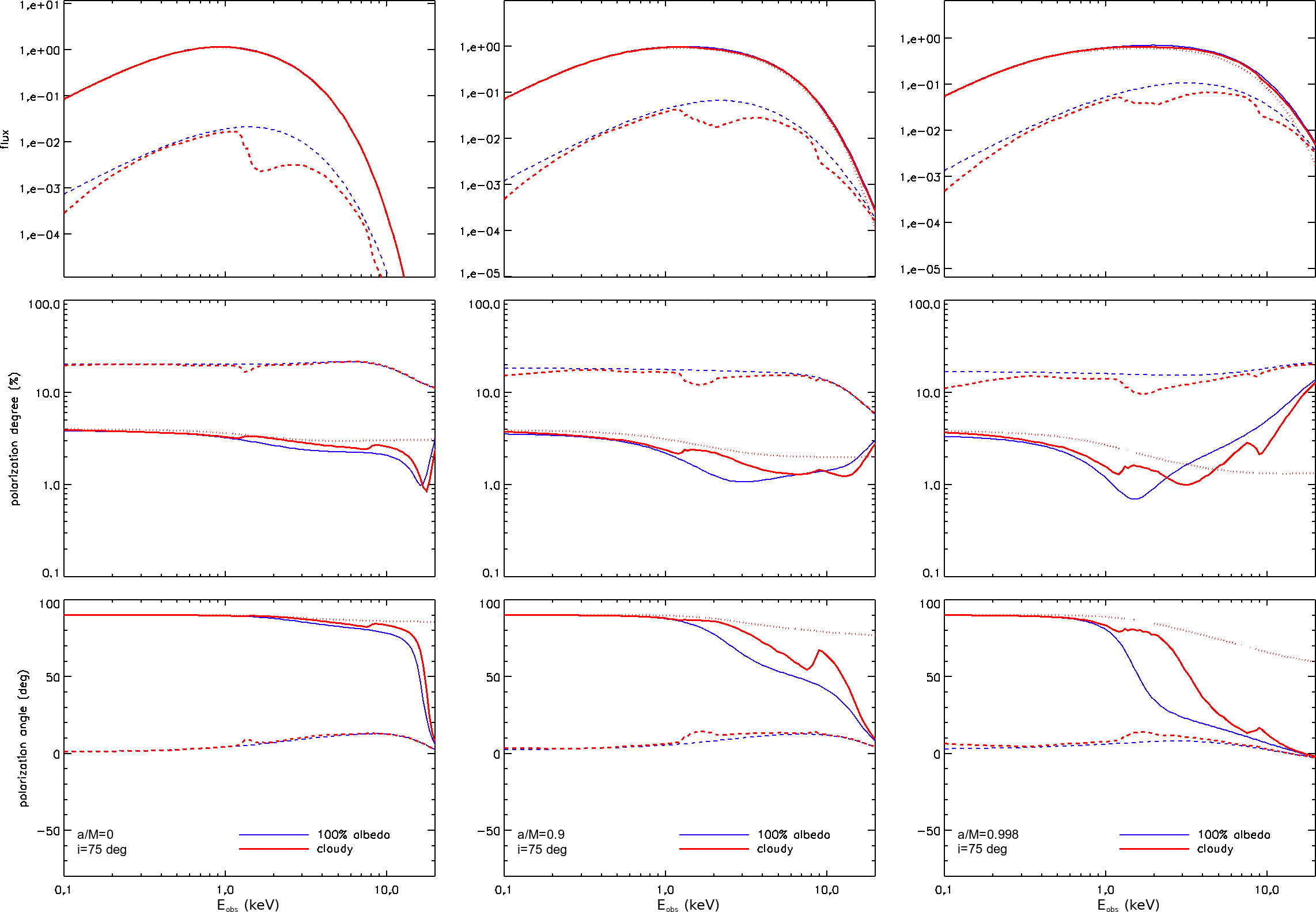
Figure 11: Spectrum (top row), polarization degree (middle row) and polarization angle (bottom row) behaviors, plotted as functions of the photon energy at the observer, for a $100\%$ albedo prescription (blue lines) and assuming the albedo profile obtained from cloudy (red lines) using the Novikov & Thorne (1973) temperature profile (equation 2), the Compère & Oliveri (2017) density profile (see Appendix B) and for $N_{\rm H}=10^{24}$ cm^-2. The values of the other parameters and line styles are taken as in Figure 1.

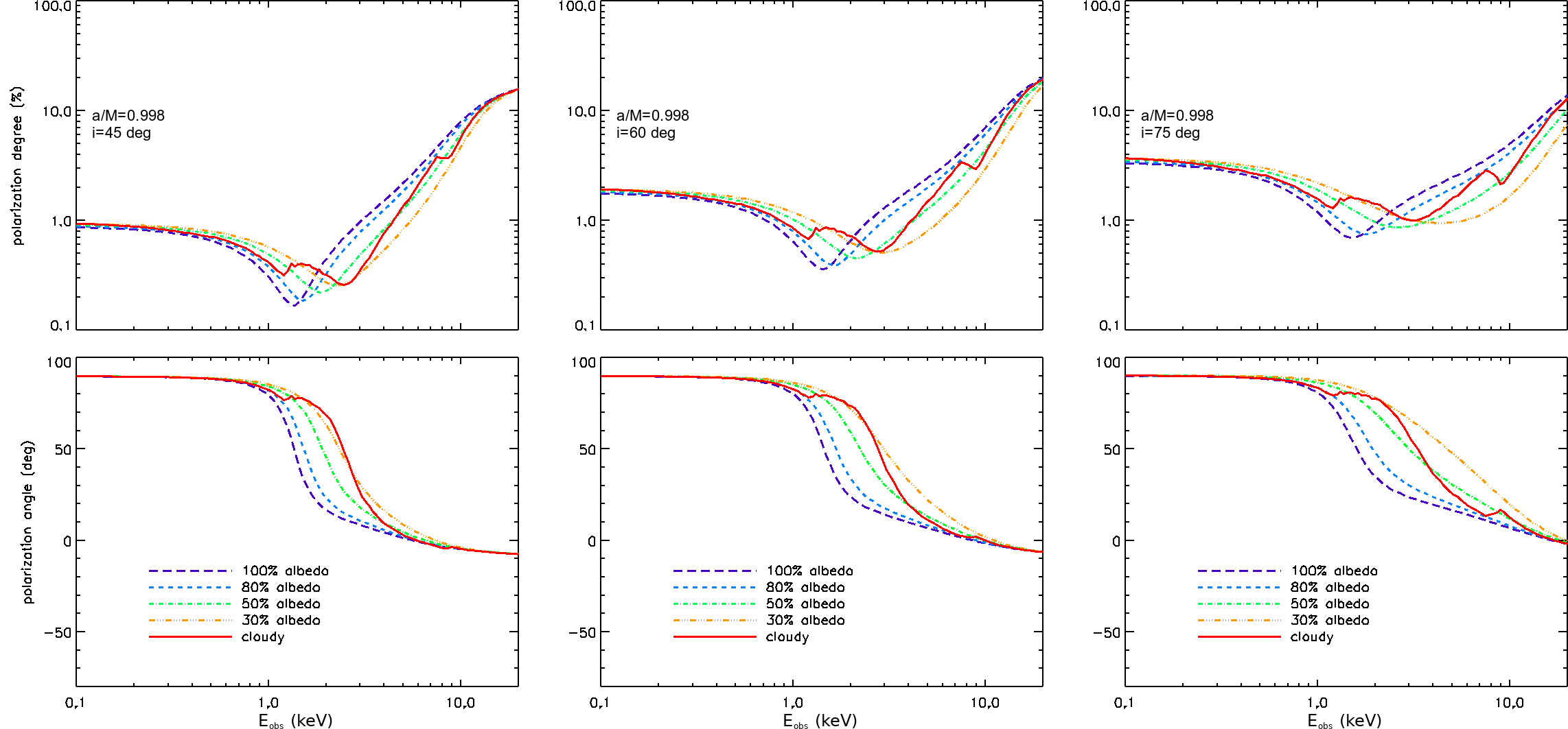
Figure 12: Joint (direct $+$ returning radiation) polarization degree (top row) and angle (bottom row) plotted as functions of the photon energy at the observer for constant $100\%$ (blue, long dashed), $80\%$ (cyan, short dashed), $50\%$ (green, dash-dotted) and $30\%$ (orange, dash-double dotted) albedo prescriptions, as well as for the albedo profile produced by cloudy (red, solid), reported in Figures 8–10. The BH spin is taken as $0.998$, while the observer’s line-of-sight inclination is $45^{\circ}$ (left), $60^{\circ}$ (center) and $75^{\circ}$ (right). The values of the other parameters are taken as in Figure 1.

A critical simplification we assumed so far in our work is that of considering a constant, $100\%$ albedo prescription at the disk surface (which implies that returning photons are all reflected towards the observer). Although computing a self-consistent ionization profile for the disk is beyond the scope of this paper (and it will be addressed in a future work), here we tried to relax the constraint on the albedo, at least in a simplified way, with the purpose to convey a sense about the effects that can be produced on spectra and polarization observables when these aspects are properly taken into account.

4.3.1 Albedo profile

In order to calculate a more realistic albedo profile for the disk surface, we use the version 17.00 of cloudy, last described by Ferland et al. (2017), a code to simulate the micro-physical processes that occur in astrophysical clouds, allowing for the prediction of the spectral properties of the radiation field that emerges (or is reflected from) these clouds. More in detail, we exploit the coronal setup, in which the gas which composes the medium is assumed to be ionized due to mutual collisions. Input parameters of each run are the (constant) gas kynetic temperature $T$ and the total (i.e. ionic, atomic and molecular) hydrogen density $n({\rm H})$. One should also provide to the code a value of the hydrogen column density $N_{\rm H}$ at which calculations are stopped. In this respect, we take in the following $N_{\rm H}=10^{24}$ cm^-2, which corresponds to $\tau\sim 1$ for Compton scattering (i.e. the process we are mainly interested for in the disk); this is tantamount to consider the layer in which most of scatterings happen. The output is a text file containing the values of the scattering, absorption and total opacities and the albedo parameter as functions of the energy, for the values of temperature and densities specified in input. For coherence with the results discussed above, we use the Novikov & Thorne (1973) profile given in equation (2) to describe the variation of the temperature with the radial distance from the center. For the density, instead, we used the formulae reported in Compère & Oliveri 2017, which give the local density profile in the inner, middle and outer regions of a general relativistic, standard disk (see Figure 10, bottom row, and Appendix B for more details).

The albedo profile is then computed by cloudy after having specified the values of temperature $T(r)$ and density $\rho(r)$ for each radial patch (with $r$ the radial distance). Results for the energy-dependent albedo profile $A(E_{\mathrm{loc}})$ obtained for different radial patches in the cases of $a=0$ (left), $0.9$ (center) and $0.998$ (right) are shown in Figure 8. As it can be clearly seen, in all the cases explored the simplifying assumption of 100% albedo turns out to be a good approximation only at very high energies, i.e. $E_{\rm loc}\approx 10$–$100$ keV. Elsewhere, the albedo significantly deviates from unity (except for some values of $r$ at lower energies), especially in the $0.1$–$10$ keV band, which is indeed the working energy range of the forthcoming X-ray polarimeters like IXPE. Here different line features appear, more or less visible depending on the BH spin and radial distance, such as the clear iron absorption edge which occurs at around $\sim 6$–$7$ keV (see e.g. Young, Ross & Fabian, 1998). Plots in Figure 9 give a more exhaustive view on how the albedo profile depends on the density of the slab in which calculations are performed. In this case the outputs are obtained for $a=0.998$, three different values of the temperature, i.e. those corresponding to $r=2$ (left), $5$ (middle) and $10\,r_{\rm g}$ (right) according to the Novikov & Thorne (1973) temperature profile, and different values of the total hydrogen density $n({\rm H})$ between $10^{15}$ and $10^{23}$ cm^-3. The plots show that the dependence of $A(E_{\mathrm{loc}})$ on the density is stronger at low energies, where it exhibits an increasing behavior by decreasing $n({\rm H})$. In particular, it attains values close to $0$ at around $0.1$ keV for particle densities in excess of $10^{22}$–$10^{23}$ cm^-3, especially for lower temperatures (i.e. for larger radial distances, see the right panel). On the other hand, at higher energies ($\ga 10$–$20$ keV) the albedo tends to reach the same value ($\approx 1$) in the entire range of densities explored.

The top row of Figure 10 finally shows the cloudy albedo profile as a function of the radial distance $A(r)$ for the same three values of $a$ discussed in Figure 8 and assuming the temperature and density profiles expressed by equations (2) and (47), resepctively. The outputs for five different local energies, covering the $1$–$10$ keV band, are shown. Also in this case an overall reduction of the albedo with respect to $100\%$, is shown, with in general a decreasing behavior as a function of the radial distance (with the only exception at $E_{\mathrm{loc}}\approx 10$ keV, where $A(r)$ is essentially constant at $\approx 0.4$ over the entire radial range considered. A maximum, where the albedo attains a value close to $1$, can be observed at energies $E_{\mathrm{loc}}\sim 1$ keV as the innermost stable circualr orbit is approached, essentially in correspondence with the peaks of both the temperature and density profiles (see bottom row). This maximum looks rather broadened for energies close to $E_{\mathrm{loc}}\approx 1$ keV, where the albedo remains at around $100\%$ up to a distance of $20$–$30\,r_{\rm g}$ from the center.

4.3.2 Results

For coherence with the results discussed previously (see §4.1 and 4.2), the albedo profiles obtained from cloudy are firstly interpolated over the energy grid used for kyn simulations and then stored in different fits files, according to the value of the BH spin. Eventually, returning radiation Stokes parameters are convolved with the correspondent value of the albedo for each energy and radial bin, so that, at each local energy $E_{\mathrm{loc}}$, it is

$$i_{\mathrm{loc}}(r,\phi) =i^{\mathrm{dir}}_{\mathrm{loc}}(r,\phi)+i^{\mathrm{ret}}_{\mathrm{loc}}(r)A(r)$$

$$q_{\mathrm{loc}}(r,\phi) =q^{\mathrm{dir}}_{\mathrm{loc}}(r,\phi)+q^{\mathrm{ret}}_{\mathrm{loc}}(r)A(r)$$

$$u_{\mathrm{loc}}(r,\phi) =u^{\mathrm{dir}}_{\mathrm{loc}}(r,\phi)+u^{\mathrm{ret}}_{\mathrm{loc}}(r)A(r)\,,$$ (15)

where $i_{\mathrm{loc}}$, $q_{\mathrm{loc}}$ and $u_{\mathrm{loc}}$ are the energy-dependent Stokes parameters defined in §3.2.

To provide an example of how including a more realistic albedo profile can modify the behaviors of spectral and polarization properties of radiation collected from stellar-mass BH accretion disks, we report in Figure 11 (red lines) the results obtained for the same values of the input parameters as in Figure 1, where the albedo was assumed to be $100\%$ for every energy and radial bin (behaviors of Figure 1 are also reported and marked in blue in Figure 11 for ease of comparison). It can be noticed that, although returning photon spectra turn out to be strongly affected by the inclusion of a more complex albedo profile, total spectra are practically unchanged. This follows from the fact that the ratio between the returning and the direct photon numbers is quite small ($\approx 10^{-2}$–$10^{-3}$) over the almost entire energy range considered. As noticed in §4.1, the only exception occurs at very high energies ($\ga 10$ keV), where photons are mostly emitted from regions closer to $r_{\rm ms}$ (see §4.1). However, as shown in Figure 10, for $r\rightarrow r_{\rm ms}$ and $E_{\mathrm{loc}}\ga 10$ keV the albedo attains values close to $100\%$ at essentially any of the BH spins considered. For this reason, small effects on the spectra are anyway expected also at high values of $E_{\mathrm{obs}}$. Effects on polarization degree and angle trends are instead more pronounced. This is especially visible for higher BH spins ($a=0.9$ and $a=0.998$), when returning radiation contributions start to be important already at $E_{\mathrm{obs}}\sim 1$ keV. More in details, looking at the polarization angle plots (bottom row), the most important difference with respect to the $100\%$ albedo case concerns the swing which occurs when returning radiation contributions start to be dominant over the direct radiation ones. This appears to be rather broadened and in general shifted towards higher energies when the cloudy albedo profile is included. This also impacts the behavior of the polarization degree (middle row), with the minimum which is moved as well to higher energies.

In order to better investigate how indeed these particular features (both discussed in §4.1) in the polarization observable plots are modified by considering a more realistic albedo prescription, we report in Figure 12 the energy-dependent behaviors of polarization degree and angle as observed at infinity for different albedo profiles: constant $100\%$, $80\%$, $50\%$ and $30\%$ together with that obtained in output from cloudy (see Figure 8). Here the only case of $a=0.998$ is explored, with different observer’s inclinations ($i=45^{\circ}$, $60^{\circ}$ and $75^{\circ}$).While no significant changes occur by changing $i$, it clearly turns out that the effect on the polarization observables of reducing the albedo at the disk surface is mainly that of moving the minimum of the polarization degree and the swing of the polarization angle towards higher energies. This can be easily explained by the fact that convolving an albedo smaller than $1$ to the returning photon Stokes parameters acts in further suppressing the contribution of returning radiation with respect to that of the direct one (see e.g. the top row of Figure 11). Hence, the energy at which returning radiation starts to dominate over the direct component consequently raises, moving forward the minimum of the polarization degree and the transition in the polarization angle.

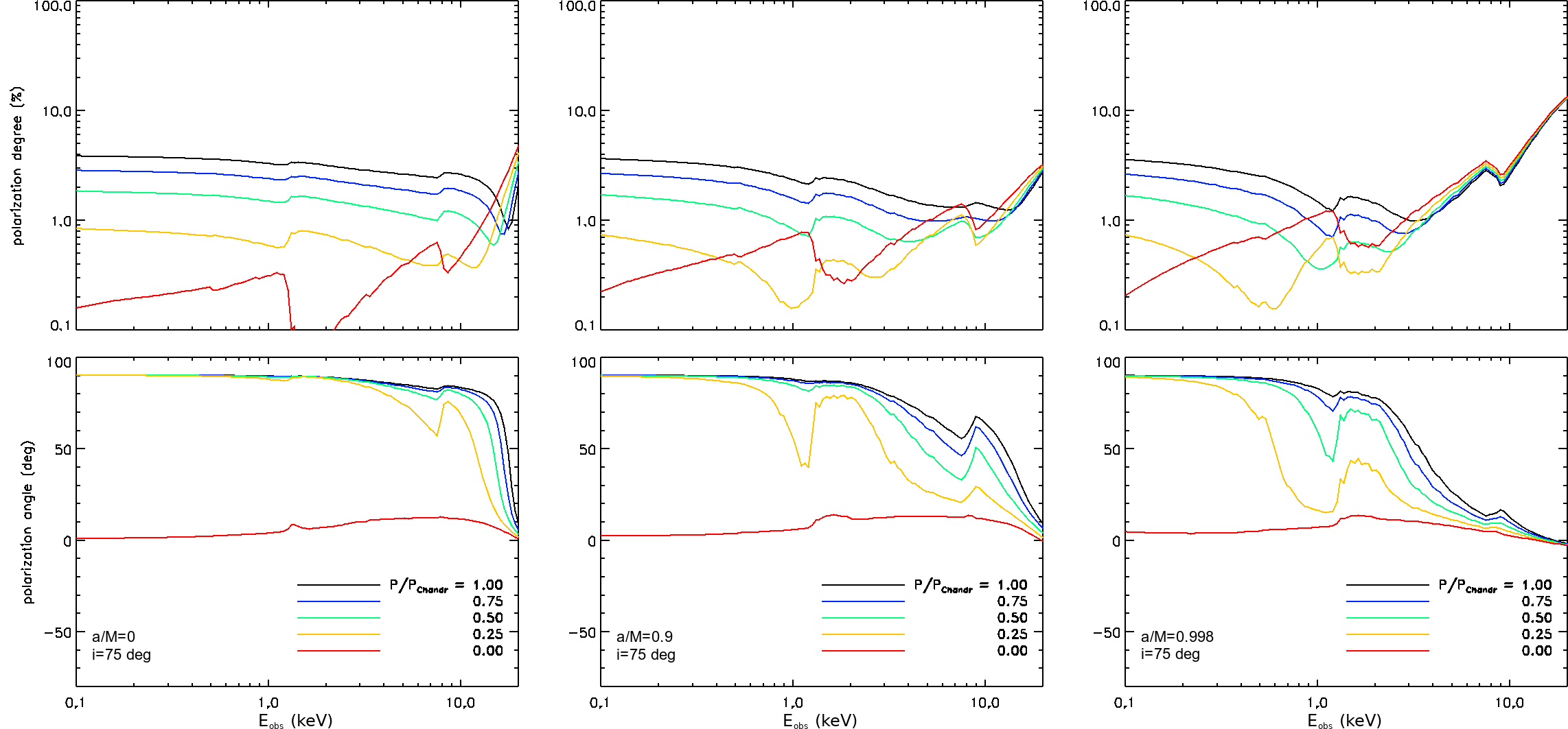
Figure 13: Joint (direct $+$ returning radiation) polarization degree (top row) and angle (bottom row), plotted as functions of the photon energy at the observer, for the same albedo profile used in Figure 11 and for direct radiation polarized at different degrees: $P^{\mathrm{dir}}_{\mathrm{loc}}=P_{\rm Chandr}$ (black), $0.75P_{\rm Chandr}$ (blue), $0.5P_{\rm Chandr}$ (green), $0.25P_{\rm Chandr}$ (orange) and $0$ (red), where $P_{\rm Chandr}$ denotes the polarization pattern expected from Chandrasekhar (1960). The values of the input parameters are taken as in Figure 1.

As well as affecting returning radiation, the absorption caused by the ionization of the disk material can be reasonably expected to change also the polarization properties of the emerging radiation. Remarking once more that a complete treatment of ionization in the disk is outside the scope of this paper, we resort to artificially reduce the polarization degree of direct photons in order to mimic this possible effect. To this aim we performed a number of simulations for which the direct radiation polarization degree ranges from $P^{\mathrm{dir}}_{\mathrm{loc}}=P_{\rm Chandr}$ (i.e. following Chandrasekhar’s, 1960, formulae) down to $0$ (i.e. unpolarized emerging light). Results, obtained for the same values of parameters assumed in Figure 11, are illustrated in Figure 13, which shows the energy-dependent polarization observables as observed at infinity. As expected, the observed polarization degree turns out to decrease, in general, by decreasing the polarization fraction of the emerging radiation. However, when photons emitted from the disk are originally unpolarized, the collected radiation may counter-intuitively result even more polarized than for non-zero intrinsic polarization. This behavior, already discussed in §4.1 commenting Figure 6, can be clearly seen looking at the red curves in the top row of Figure 13. An explanation can actually be extracted from the polarization angle plots (bottom row), where, as noticed for those reported in Figures 11 and 12, the addition of a non-trivial albedo profile broadens the range in energy over which the polarization angle swing extends. Since, on the other hand, the polarization angle is rather constant when direct radiation is assumed to be unpolarized (so that no transition occurs at all), the correspondent polarization fraction is much less reduced than for the other cases, in which instead the variation of the polarization angle with the energy is more significant.

5 Discussion and conclusions

In this work we have revisited the problem of the spectral and polarization properties of radiation emitted from stellar-mass BH accretion disks in the soft state, considering the contribution of returning radiation (i.e. photons which are bent by the strong BH gravity to return to the disk before being reflected towards the observer) alongside that of direct radiation (i.e. photons that arrive directly to the observer once emitted from the disk surface). To this aim we first added to the kyn package Dovčiak (2004) a specific module, exploiting the c++ code selfirr (based on the ray-tracing sim5 package, see Bursa, 2017) to calculate all the possible null geodesics along which photons can travel between two different points on the disk surface (assuming a Kerr space-time, see section 2). Secondly, we have checked that the results of our simulations were compatible with those discussed in previous works (e.g. Schnittman & Krolik, 2009; Krawczynski, 2012) which already considered returning radiation in their calculations. As widely discussed in section 4.1, the comparison has revealed an overall good agreement over a large range of input parameters, with only some discrepancies in the case of $a=0.9$, occurring essentially at an energy higher then $20$ keV. We remarked that statistics at such high energies would be definitively too low for the present polarimetry techniques (see e.g. Costa et al., 2001; Bellazzini et al., 2010) to provide conclusive results.

Using the Monte Carlo code stokes, we have been able to investigate how spectral and polarization properties are modified by varying the optical depth of the (pure-scattering) atmosphere assumed to cover the disk (see §4.2). We found that the trends of the polarization observables are rather similar to those obtained for an infinite optical depth when $\tau\ga 5$. On the other hand, a significantly higher polarization fraction (even by a factor of $\sim 6$–$10$ at low energies) can be expected when values of $\tau$ smaller than $1$ are considered; a transition between the two regimes occurs at around $\tau\sim 2$ (in agreement with the results already discussed by Dovčiak et al., 2008). This certainly changes the expected polarization signature of soft-state BH accretion disks in the $2$–$10$ keV energy range, which will be attained by the next-generation polarimeters like IXPE Weisskopf et al. (2013). Moreover, if future polarimeters capable to investigate polarization also at energies $\approx 0.1$–$2$ keV (like XPP, see Krawczynski et al., 2019) will be deployed in the next years, this behavior can be used in principle to obtain information on the optical properties of the medium from which photons have been emitted.

Without entering into details (a more complete treatment of the ionization profile in the disk will be addressed in a future work), we then started to make a more realistic assumption for the disk albedo profile, going beyond the simplified prescription of taking it constant at $100\%$. To this aim we used the code cloudy Ferland et al. (2017), assuming that ionization in the disk material is due essentially to mutual collisions between its particles. The albedo profiles obtained from cloudy were then convolved with the returning radiation Stokes parameters computed by kyn. The plots reported in §4.3.2 offer an illustration of the effects of a more realistic albedo prescription on both spectra and polarization observables. A comparison with the case discussed in section 4.1 shows that introducing in the calculations a more complicated albedo profile can significantly alter the behavior of polarization degree and angle with respect to the simplifying $100\%$-albedo prescription. This can in particular affect the constraints on BH spin and inclination angle which may be extracted from polarization measurements (see Figure 12).

Finally, we tried to reproduce the possible effects of the disk ionization also on the polarization properties of the emerging radiation. As a first attempt (which will be also investigated more in depth in a future work), we resorted to reduce the polarization degree assigned to the direct radiation component in our simulations, starting from the pure-scattering polarization pattern predicted by Chandrasekhar (1960) up to assuming an unpolarized radiation (see Figure 13). Such effects turned out to be indeed quite important, especially in the case of weakly-polarized direct photons, for which radiation collected at infinity may result even more polarized with respect to the case of Chandrasekhar-like intrinsic polarization.

To conclude, on the wave of previous works (see e.g. Dovčiak et al., 2008; Schnittman & Krolik, 2009; Krawczynski, 2012; Schnittman & Krolik, 2013), we confirm that X-ray polarization measurements can be crucial in extending our knowledge about stellar-mass BH accretion disks in the soft state. However, when the optical structure of the disk is considered in more detail (e.g. taking the surface optical depth and the disk ionization as free parameters of the problem), the simple scenario depicted under the assumptions of $\tau=1$ and $100\%$ albedo may be not the right description. However, we point out that there are several effects, we did not consider in the present work, which can somehow mitigate the degeneracy introduced by considering absorption in the disk material. For example, the contributions due to magnetic pressure in determining the vertical structure of the disk or the photoionization due to radiation coming from an external corona, may significantly increase the ionization fraction and therefore increase the albedo as well. Moreover, deeper investigations, which are outside the scope of the present paper, are requested in order to provide a more realistic picture of these kind of sources through the joint effort of spectroscopy and X-ray polarimetry. This involves a self-consistent treatment of ionization in the disk material, a more general prescription for the vertical structure of the disk (see Appendix B) and the inclusion of absorption effects in the radiative transfer calculations of polarized thermal photons (i.e. not only for the reflected ones). We are planning to address these issues in future works.

The sensitive functional dependence of the polarization observables (seen as functions of the photon energy) on the physical state of the accretion disk should allow us to set more stringent constraints on the models of the accretion medium along with the effects of General Relativity. This makes it possible in future, also exploiting the capabilities of instruments like IXPE, to reduce the inherent degeneracies of these models and to measure the parameters, including the BH spin.

Appendix A Diffuse reflection formulae

Chandrasekhar’s (1960) diffuse reflection law can be expressed as

$$\left(\begin{array}[]{c}I_{\rm l}\\ I_{\rm r}\\ U\end{array}\right) =\frac{1}{4\mu}\boldsymbol{Q}\boldsymbol{S}(\mu,\varphi;\bar{\mu}_{\rm i},\bar{\varphi}_{\rm i})\left(\begin{array}[]{c}F_{\rm l}\\ F_{\rm r}\\ F_{\rm U}\end{array}\right)\,,$$ (22)

where $I_{\rm l}$, $I_{\rm r}$ and $U$ are the (number) intensities which characterize the radiation field ($l$ and $r$ refer to two mutually orthogonal directions, in the plane made by the disk symmetry axis and the observer’s line-of-sight and perpendicular to this plane, respectively), $F_{\rm l}$, $F_{\rm r}$ and $F_{\rm U}$ are the correspondent (number) fluxes, $\mu=\cos\theta$ ($\bar{\mu}_{\rm i}=\cos\bar{\theta}_{\rm i}$) is the cosine of the emission (incidence) angle that the propagation direction makes with the disk symmetry axis and

$$\boldsymbol{Q} =\left(\begin{array}[]{ccc}1&0&0\\ 0&1&0\\ 0&0&2\end{array}\right)\,.$$ (26)

The elements of the matrix

$$\boldsymbol{S}(\mu,\varphi;\bar{\mu}_{\rm i},\bar{\varphi}_{\rm i}) =\frac{3}{4}\frac{\bar{\mu}_{\rm i}\mu}{\mu+\bar{\mu}_{\rm i}}\left(\begin{array}[]{ccc}S_{11}&S_{12}&S_{13}\\ S_{21}&S_{22}&S_{23}\\ S_{31}&S_{32}&S_{33}\end{array}\right)$$ (30)

are given by the following expressions:

$$S_{11} =\psi(\mu)\psi(\bar{\mu}_{\rm i})+2\phi(\mu)\phi(\bar{\mu}_{\rm i})$$

$$-4\mu\bar{\mu}_{\rm i}[(1-\mu^{2})(1-\bar{\mu}_{\rm i}^{2})]^{1/2}H^{(1)}(\mu)H^{(1)}(\bar{\mu}_{\rm i})\cos(\bar{\varphi}_{\rm i}-\varphi)$$

$$+\mu^{2}\bar{\mu}_{\rm i}^{2}H^{(2)}(\mu)H^{(2)}(\bar{\mu}_{\rm i})\cos[2(\bar{\varphi}_{\rm i}-\varphi)]\,;$$ (31)

$$S_{12} =\psi(\mu)\chi(\bar{\mu}_{\rm i})+2\phi(\mu)\zeta(\bar{\mu}_{\rm i})$$

$$-\mu^{2}H^{(2)}(\mu)H^{(2)}(\bar{\mu}_{\rm i})\cos[2(\bar{\varphi}_{\rm i}-\varphi)]\,;$$ (32)

$$S_{13} =2\mu[(1-\mu^{2})(1-\bar{\mu}_{\rm i}^{2})]^{1/2}H^{(1)}(\mu)H^{(1)}(\bar{\mu}_{\rm i})\sin(\bar{\varphi}_{\rm i}-\varphi)$$

$$-\mu^{2}\bar{\mu}_{\rm i}H^{(2)}(\mu)H^{(2)}(\bar{\mu}_{\rm i})\sin[2(\bar{\varphi}_{\rm i}-\varphi)]\,;$$ (33)

$$S_{21} =\chi(\mu)\psi(\bar{\mu}_{\rm i})+2\zeta(\mu)\phi(\bar{\mu}_{\rm i})$$

$$-\bar{\mu}_{\rm i}^{2}H^{(2)}(\mu)H^{(2)}(\bar{\mu}_{\rm i})\cos[2(\bar{\varphi}_{\rm i}-\varphi)]\,;$$ (34)

$$S_{22} =\chi(\mu)\chi(\bar{\mu}_{\rm i})+2\zeta(\mu)\zeta(\bar{\mu}_{\rm i})$$

$$+H^{(2)}(\mu)H^{(2)}(\bar{\mu}_{\rm i})\cos[2(\bar{\varphi}_{\rm i}-\varphi)]\,;$$ (35)

$$S_{23} =\bar{\mu}_{\rm i}H^{(2)}(\mu)H^{(2)}(\bar{\mu}_{\rm i})\sin[2(\bar{\varphi}_{\rm i}-\varphi)]\,;$$ (36)

$$S_{31} =2\bar{\mu}_{\rm i}[(1-\mu^{2})(1-\bar{\mu}_{\rm i}^{2})]^{1/2}H^{(1)}(\mu)H^{(1)}(\bar{\mu}_{\rm i})\sin(\bar{\varphi}_{\rm i}-\varphi)$$

$$-\mu\bar{\mu}_{\rm i}^{2}H^{(2)}(\mu)H^{(2)}(\bar{\mu}_{\rm i})\sin[2(\bar{\varphi}_{\rm i}-\varphi)]\,;$$ (37)

$$S_{32} =\mu H^{(2)}(\mu)H^{(2)}(\bar{\mu}_{\rm i})\sin[2(\bar{\varphi}_{\rm i}-\varphi)]\,;$$ (38)

$$S_{33} =[(1-\mu^{2})(1-\bar{\mu}_{\rm i}^{2})]^{1/2}H^{(1)}(\mu)H^{(1)}(\bar{\mu}_{\rm i})\cos(\bar{\varphi}_{\rm i}-\varphi)$$

$$-\mu\bar{\mu}_{\rm i}H^{(2)}(\mu)H^{(2)}(\bar{\mu}_{\rm i})\cos[2(\bar{\varphi}_{\rm i}-\varphi)]\,.$$ (39)

The values that the special functions $\psi(\mu)$, $\phi(\mu)$, $\chi(\mu)$, $\zeta(\mu)$, $H^{(1)}(\mu)$ and $H^{(2)}(\mu)$ take on a descrete grid of $\mu$ are reported in Table XXV of Chandrasekhar (1960).

Stokes parameters can be obtained from $I_{\rm l}$, $I_{\rm r}$ and $U$ given in equation (22) through

$$\bar{i}_{\mathrm{refl}} =I_{\rm l}+I_{\rm r}$$

$$\bar{q}_{\mathrm{refl}} =I_{\rm l}-I_{\rm r}$$

$$\bar{u}_{\mathrm{refl}} =U\,,$$ (40)

while the components of the Stokes vectors $\boldsymbol{\bar{s}}_{\mathrm{refl}}(0,-)$, $\boldsymbol{\bar{s}}_{\mathrm{refl}}(1,0)$ and $\boldsymbol{\bar{s}}_{\mathrm{refl}}(1,\pi/4)$ used in equation (3.2) can be obtained from equation (22) by placing $F_{\rm l}=F_{\rm r}=f_{\mathrm{loc}}/2$, $F_{\rm U}=0$ for unpolarized light, $F_{\rm l}=f_{\mathrm{loc}}$, $F_{\rm r}=F_{\rm U}=0$ for vertically-polarized light and $F_{\rm l}=F_{\rm r}=f_{\mathrm{loc}}/2$, $F_{\rm U}=f_{\mathrm{loc}}$ for $45^{\circ}$-polarized light.

Appendix B Disk density profile

In order to calculate coherently the albedo profile of the disk with cloudy, we adopted the density profile given by Compère & Oliveri (2017), who revised the standard disk local structure formulae originally discussed by Novikov & Thorne (1973, see also and ) for both stellar-mass and supermassive BHs. For the sake of a better readability, we reported in the following the main expressions we used in our calculations. The disk is divided into three main regions, according to what mechanism dominates the transfer of radiation in the disk material. In the inner (or edge) region, where it holds

$$\frac{p_{\rm gas}}{p_{\rm rad}} =(2.6\times 10^{-5})\,\alpha^{-1/4}M_{*}^{7/4}\dot{M}_{*}^{-2}$$

$$\ \ \ \ \times x^{29/4}\mathcal{C}^{9/4}\mathcal{D}^{-1/4}\mathcal{R}^{5/4}\mathcal{P}^{-2}\ll 1\,,$$

$$\frac{\kappa_{\rm ff}}{\kappa_{\rm es}} =(2.2\times 10^{-8})\,\alpha^{-1/8}M_{*}^{15/8}\dot{M}_{*}^{-2}$$

$$\ \ \ \ \times x^{61/8}\mathcal{C}^{17/8}\mathcal{D}^{-1/8}\mathcal{R}^{9/8}\mathcal{P}^{-2}\ll 1\,,$$ (41)

with $p_{\rm gas}$ ($p_{\rm rad}$) the gas (radiation) pressure and $\kappa_{\rm ff}$ ($\kappa_{\rm es}$) the free-free (scattering) opacity, the (equatorial) hydrogen density $n_{0}(\rm H)$ is given by

$$n_{0}({\rm H})_{\rm inn} =(1.50\times 10^{19}\,{\rm cm^{-3}})\,\alpha^{-1}M_{*}\dot{M}_{*}^{-2}$$

$$\ \ \ \ \times x^{5}\mathcal{C}^{3}\mathcal{D}^{-1}\mathcal{R}^{2}\mathcal{P}^{-2}\,.$$ (42)

Then, in the middle region, where

$$\frac{p_{\rm rad}}{p_{\rm gas}} =(69)\,\alpha^{1/10}M_{*}^{-7/10}\dot{M}_{*}^{4/5}$$

$$\ \ \ \ \times x^{-29/10}\mathcal{C}^{-9/10}\mathcal{D}^{1/10}\mathcal{R}^{-1/2}\mathcal{P}^{4/5}\ll 1\,,$$

$$\frac{\kappa_{\rm ff}}{\kappa_{\rm es}} =(4.4\times 10^{-6})\,M_{*}\dot{M}_{*}^{-1}$$

$$\ \ \ \ \times x^{4}\mathcal{C}\mathcal{R}^{1/2}\mathcal{P}^{-1}\ll 1\,,$$ (43)

one has

$$n_{0}({\rm H})_{\rm mid} =(4.86\times 10^{24}\,{\rm cm^{-3}})\,\alpha^{-7/10}M_{*}^{-11/10}\dot{M}_{*}^{2/5}$$

$$\ \ \ \ \times x^{-37/10}\mathcal{C}^{3/10}\mathcal{D}^{-7/10}\mathcal{R}^{1/2}\mathcal{P}^{2/5}\,.$$ (44)

Finally, in the outer region, where

$$\frac{p_{\rm rad}}{p_{\rm gas}} =(0.27)\,\alpha^{1/10}M_{*}^{-1/4}\dot{M}_{*}^{7/20}$$

$$\ \ \ \ \times x^{-11/10}\mathcal{C}^{-9/20}\mathcal{D}^{1/10}\mathcal{R}^{-11/40}\mathcal{P}^{7/20}\ll 1\,,$$

$$\frac{\kappa_{\rm es}}{\kappa_{\rm ff}} =(4.8\times 10^{2})\,M_{*}^{-1/2}\dot{M}_{*}^{1/2}$$

$$\ \ \ \ \times x^{-2}\mathcal{C}^{-1/2}\mathcal{R}^{-1/4}\mathcal{P}^{1/2}\ll 1\,,$$ (45)

it is

$$n_{0}({\rm H})_{\rm out} =(3.06\times 10^{25}\,{\rm cm^{-3}})\,\alpha^{-7/10}M_{*}^{-5/4}\dot{M}_{*}^{11/20}$$

$$\ \ \ \ \times x^{-43/10}\mathcal{C}^{3/20}\mathcal{D}^{-7/10}\mathcal{R}^{17/40}\mathcal{P}^{11/20}\,.$$ (46)

In equations (B)–(B) we have taken $M_{*}=M/3M_{\odot}$, $\dot{M}_{*}$ is the mass accretion rate in units of $10^{17}$ g s^-1 and $x=(r/r_{\rm g})^{1/2}$. We refer the reader to Compère & Oliveri (2017) for the complete expressions of the functions $\mathcal{C}$, $\mathcal{D}$, $\mathcal{R}$ and $\mathcal{P}$. Transitions among the different regions are determined by checking the validity of conditions (B), (B) and (B).

In order to obtain the hydrogen density $n({\rm H})$, calculated at the altitude $z_{*}$ over the equatorial plane where returning photons are eventually absorbed by the disk material, we need to specify the vertical structure of the disk. For the sake of simplicity, and since a full treatment of the disk vertical structure is beyond the scope of this work, we adopted a simple gaussian prescription for the density (see Shakura & Sunayev, 1973),

$$n(\rm H) =n_{0}({\rm H})\exp\left(-\frac{z^{2}}{h^{2}}\right)\,,$$ (47)

where $h$ denotes the typical disk height at the distance $r$ from the center. In the three above-mentioned regions it turns out to be

$$h_{\rm inn} =(0.5\,r_{\rm g})M_{*}^{-1}\,\dot{M}_{*}$$

$$\ \ \ \ \times x^{-3}\mathcal{C}^{-1}\mathcal{R}^{-1}\mathcal{P}$$

$$h_{\rm mid} =(7.0\times 10^{-3}\,r_{\rm g})\,\alpha^{-1/10}M_{*}^{-3/10}\dot{M}_{*}^{1/5}$$

$$\ \ \ \ \times x^{-1/10}\mathcal{C}^{-1/10}\mathcal{D}^{-1/10}\mathcal{R}^{-1/2}\mathcal{P}^{1/5}$$

$$h_{\rm out} =(3.8\times 10^{-3}\,r_{\rm g})\,\alpha^{-1/10}M_{*}^{-1/4}\dot{M}_{*}^{3/20}$$

$$\ \ \ \ \times x^{1/10}\mathcal{C}^{-1/20}\mathcal{D}^{-1/10}\mathcal{R}^{-19/40}\mathcal{P}^{3/20}\,.$$ (48)

A more general profile for the vertical structure (still within the assumption of geometrically thin disks, see e.g. Davis & Hubeny, 2006) will be addressed in future investigations.

We then resorted to choose $z_{*}$ in such a way that the scattering optical depth calculated up to infinity is equal to $1$, i.e.

$$\tau =\int_{z_{*}}^{\infty}n_{0}({\rm H})\exp\left(-\frac{z^{2}}{h^{2}}\right)\sigma_{\rm T}\mathrm{d}z\equiv 1\,,$$ (49)

with $\sigma_{\rm T}$ the Thomson cross section. Solving numerically equation (49) one obtains

$$z_{*}(r) =h(r)\,{\rm erf}^{-1}\left[1-\frac{2}{n_{0}({\rm H},r)h(r)\sigma_{\rm T}\sqrt{\pi}}\right]\,,$$ (50)

where ${\rm erf}^{-1}$ denotes the inverse of the error function.

In all the expressions above, free parameters are the BH mass $M$ and accretion rate $\dot{M}$, the parameter $\alpha$ and the height $h_{0}$ of the disk at the innermost stable circular orbit. Throughout our calculations we take $\alpha=0.2$ (see Compère & Oliveri, 2017) and

$$h_{0}^{\rm inn} =0.002\,r_{\rm g}$$

$$h_{0}^{\rm mid} =(1.8\times 10^{-3}\,r_{\rm g})\,\alpha^{1/8}M_{*}^{-3/8}\dot{M}_{*}^{1/4}$$

$$\ \ \ \ \times x_{0}^{1/8}\mathcal{C}_{0}^{-1/8}\mathcal{R}_{0}^{-1/2}$$

$$h_{0}^{\rm out} =(1.3\times 10^{-3}\,r_{\rm g})\,\alpha^{1/17}M_{*}^{-5/17}\dot{M}_{*}^{3/17}$$

$$\ \ \ \ \times x_{0}^{5/17}\mathcal{C}_{0}^{-1/17}\mathcal{D}_{0}^{-1/34}\mathcal{R}_{0}^{-8/17}\,,$$ (51)

where a $0$ subscript denotes quantities calculated at $r=r_{\rm ms}$. The chosen values of $M$ and $\dot{M}$ are specified in the text.

References

- Abbott et al. (2016) Abbott B. P. et al., 2016, Phys. Rev. Lett., 116, 241102
- Abramowicz & Fragile (2013) Abramowicz M. A., Fragile P. C., 2013, Living Rev. Relativ., 16, 1
- Agol & Krolik (2000) Agol E., Krolik J. H., 2000, ApJ, 528, 161
- Bao et al. (1997) Bao G., Hadrava P., Wiita P. J., Xiong Y., 1997, ApJ, 487, 142
- Bardeen (1970) Bardeen J. M., 1970, Nature, 226, 64
- Bardeen et al. (1972) Bardeen J. M., Press W. H., Teukolsky S. A., 1972, ApJ, 178, 347
- Bellazzini et al. (2010) Bellazzini R., Costa E., Matt G., Tagliaferri G., 2010, X-ray Polarimetry: A New Window in Astrophysics. Cambridge University Press, Cambridge
- Bursa (2017) Bursa M., 2017, in Proceedings of RAGtime 17-19: Workshops on Black Holes and Neutron Stars, Opava, Czech Republic: Z. Stuchlík, G. Török and V. Karas, 7-21
- Carter (1968) Carter B. 1968, PhRv, 174, 1559
- Chandrasekhar (1960) Chandrasekhar S., 1960, Radiative transfer, Dover, New York
- Chandrasekhar (1983) Chandrasekhar S., 1983, The Mathematical Theory of Black Holes, Oxford University Press, New York
- Compère & Oliveri (2017) Compère G., Oliveri R., 2017, MNRAS, 468, 4351
- Connors & Stark (1977) Connors P. A., Stark R. F., 1977, Nature, 269, 128
- Connors, Piran & Stark (1980) Connors P. A., Piran T., Stark R. F., 1980, ApJ, 235, 224
- Costa et al. (2001) Costa E., Soffitta P., Bellazzini R., Brez A., Lumb B., Spandre G., 2001, Nature, 411, 662
- Cunningham (1975) Cunningham C. T., 1975, ApJ, 202, 788
- Davis & El-Abd (2019) Davis S. W., El-Abd S., 2019, ApJ 874, 23
- Davis & Hubeny (2006) Davis S. W., Hubeny I., 2006, ApJS 164, 530
- Dovčiak (2004) Dovčiak M., 2004, PhD thesis, Charles Univ., Prague (astro-ph/0411605)
- Dovčiak et al. (2004a) Dovčiak M., Karas V., Matt G., 2004a, MNRAS, 355, 1005
- Dovčiak et al. (2004b) Dovčiak M., Karas V., Yaqoob T., 2004b, Ap&SS, 153, 205
- Dovčiak et al. (2004c) Dovčiak M., Karas V., Matt G., Yaqoob T., 2004c, in Hledík S., Stuchlík Z., 2004c, eds, Proc. of Workshops on Black Holes and Neutron Stars. Sileian University, Opava, p. 33
- Dovčiak et al. (2008) Dovčiak M., Muleri F., Goosmann R. W., Karas V., Matt G., 2008, MNRAS, 391, 32
- Dovčiak et al. (2011) Dovčiak M., Muleri F., Goosmann R. W., Karas V., Matt G., 2011, ApJ, 731, 75
- Ferland et al. (2017) Ferland G. J. et al., 2017, The 2017 Release Cloudy. Revista Mexicana de Astronomia y Astrofisica, 53, 385
- Goosmann & Gaskell (2007) Goosmann R. W., Gaskell C. M., 2007, A&A, 465, 129
- Graham (2016) Graham A. W., 2016, ASSL, 418, 263
- Ishihara, Takahashi & Tomimatsu (1988) Ishihara H., Takahashi M., Tomimatsu, A. 1988, Phys. Rev. D, 48, 472
- Karas (2006) Karas V., 2006, AN, 327, 961
- Kormendy & Ho (2013) Kormendy J., Ho L. C., 2013, ARA&A, 51, 511
- Krawczynski (2012) Krawczynski H., 2012, ApJ, 754, 133
- Krawczynski et al. (2019) Krawczynski H. et al., 2019, BAAS, 51, 150
- Laor et al. (1990) Laor A., Netzer H., Piran T., 1990, MNRAS, 242, 560
- Li et al. (2009) Li L.-X., Narayan R., McClintock J. E., 2009, ApJ, 691, 847
- Li et al. (2005) Li L.-X., Zimmerman E. R., Narayan R., McClintock J. E., 2005, ApJS, 157, 335
- Lynden-Bell (1969) Lynden-Bell D., 1969, Nature, 223, 690
- Marin (2018) Marin F., 2018, A&A, 615, 171
- Matt et al. (1993) Matt G., Fabian A. C., Ross R. R., 1993, MNRAS, 264, 839
- Mezcua (2017) Mezcua M., 2017, IJMPD, 2630021
- Novikov & Thorne (1973) Novikov I. D. , Thorne K. S. , 1973, in Black Holes (Les Astres Occlus), C. Dewitt, and B. S. Dewitt, 343
- Page & Thorne (1974) Page D. N., Thorne K. S., 1974, ApJ, 191, 499
- Rauch & Blandford (1994) Rauch K. P., Blandford R. D., 1994, ApJ, 421, 46
- Salpeter (1964) Salpeter E. E., 1964, ApJ, 140, 796
- Schnittman & Krolik (2009) Schnittman J. D., Krolik J. H., 2009, ApJ, 701, 1175
- Schnittman & Krolik (2010) Schnittman J. D., Krolik J. H., 2010, ApJ, 712, 908
- Schnittman et al. (2013) Schnittman J. D., Krolik J. H., Noble S. C., 2013, ApJ, 769, 156
- Schnittman & Krolik (2013) Schnittman J. D., Krolik J. H., 2013, ApJ, 777, 11
- Schödel et al. (2002) Schödel R. et al., 2002, Nature, 419, 694
- Shakura & Sunayev (1973) Shakura N. I., Sunyaev R. A., 1973, A&A, 24, 337
- Silant’ev (2002) Silant’ev N. A., 2002, A&A, 383, 326
- Silant’ev et al. (2009) Silant’ev N. A., Piotrovich M. Ye., Gnedin Yu. N., Natsvlishvili T. M., 2009, A&A, 507, 171
- Silant’ev et al. (2018) Silant’ev N. A., Alekseeva G. A., Novikov V. V., 2018, AP&SS, 363, 155
- Stark & Connors (1977) Stark R. F., Connors P. A., 1977, Nature, 266, 429
- Walker & Penrose (1970) Walker M., Penrose R., 1970, Comm. in Math. Phys., 18, 265
- Wang (2000) Wang D., 2000, CAA, 24, 13
- Weisskopf et al. (2013) Weisskopf M. C. et al., 2013, in UV, X-Ray, and Gamma-Ray Space Instrumentation for Astronomy XVIII, Proc. SPIE, 8859
- Woosley, Heger & Weaver (2002) Woosley S. E., Heger A., Weaver T. A., 2002, Rev. Mod. Phys., 74, 1015
- Young, Ross & Fabian (1998) Young A. J., Ross R. R., Fabian A. C., 1998, MNRAS, 300, L11
- Zhang, Dovčiak & Bursa (2019) Zhang W., Dovčiak M., Bursa, M., 2019, ApJ, 875, 148
- Zel’dovich & Novikov (1964) Zel’dovich Y. B., Novikov I. D., 1964, Sov. Phys. Dokl., 158, 811